


1 Introduction
Single flapping foils are commonly found in nature and can be very efficient and effective propulsors. Tandem flapping foils, where one is upstream of the other, have some potential advantages over single flapping foils due to the hind foil being located in the wake of the fore foil. Although some form of foil–wake interaction can be seen between the fins of fish (Akhtar et al. Reference Akhtar, Mittal, Lauder and Drucker2007), the parameter space of such a situation becomes larger when the fore and hind foils are able to move independently of each other. High-speed video has shown that dragonflies change the phasing of the flapping motion between their fore and hind wings depending on the flight manoeuvres that they are performing (Alexander Reference Alexander1984). Another analysis of dragonfly flight used flow visualisation to show that dragonflies use an out-of-phase motion for normal free flight, but switch to in-phase for acceleration (Thomas et al. Reference Thomas, Taylor, Srygley, Nudds and Bomphrey2004).
Previous studies have shown that the force production on the hind foil of a tandem-foil configuration is affected by the phase difference in the kinematics between the fore and hind foils (
 $\unicode[STIX]{x1D711}$
) and the inter-foil spacing (
$\unicode[STIX]{x1D711}$
) and the inter-foil spacing (
 $S$
) (Broering & Lian Reference Broering and Lian2010; Kumar & Hu Reference Kumar and Hu2011; Rival, Hass & Tropea Reference Rival, Hass and Tropea2011; Broering, Lian & Henshaw Reference Broering, Lian and Henshaw2012; Kinsey & Dumas Reference Kinsey and Dumas2012; Boschitsch, Dewey & Smits Reference Boschitsch, Dewey and Smits2014; Lian et al.
Reference Lian, Broering, Hord and Prater2014; Gong, Jia & Xi Reference Gong, Jia and Xi2015, Reference Gong, Jia and Xi2016). This effect has been addressed as ‘wake recapture’, ‘wing–wake interaction’, or ‘thrust augmentation’. For the purposes of this work, ‘performance augmentation’ is deemed the most suitable description, as this term accounts for the augmentation of both thrust and efficiency. Within these above-mentioned articles, the extent of the phase–spacing–frequency parameter space that has been explored is very limited.
$S$
) (Broering & Lian Reference Broering and Lian2010; Kumar & Hu Reference Kumar and Hu2011; Rival, Hass & Tropea Reference Rival, Hass and Tropea2011; Broering, Lian & Henshaw Reference Broering, Lian and Henshaw2012; Kinsey & Dumas Reference Kinsey and Dumas2012; Boschitsch, Dewey & Smits Reference Boschitsch, Dewey and Smits2014; Lian et al.
Reference Lian, Broering, Hord and Prater2014; Gong, Jia & Xi Reference Gong, Jia and Xi2015, Reference Gong, Jia and Xi2016). This effect has been addressed as ‘wake recapture’, ‘wing–wake interaction’, or ‘thrust augmentation’. For the purposes of this work, ‘performance augmentation’ is deemed the most suitable description, as this term accounts for the augmentation of both thrust and efficiency. Within these above-mentioned articles, the extent of the phase–spacing–frequency parameter space that has been explored is very limited.
Work has focused on the effects of phase alone (Rival et al.
Reference Rival, Hass and Tropea2011; Lian et al.
Reference Lian, Broering, Hord and Prater2014), or the effect of phase and frequency (Broering et al.
Reference Broering, Lian and Henshaw2012) or spacing and frequency (or Strouhal number,
 $St$
) (Kinsey & Dumas Reference Kinsey and Dumas2012). Many studies have investigated both the phase and spacing, but at only one flapping frequency (Kumar & Hu Reference Kumar and Hu2011; Broering & Lian Reference Broering and Lian2012; Boschitsch et al.
Reference Boschitsch, Dewey and Smits2014; Gong et al.
Reference Gong, Jia and Xi2015, Reference Gong, Jia and Xi2016). One study has considered the effects of both spacing and phase at different flapping frequencies, or Strouhal numbers (Broering & Lian Reference Broering and Lian2010), although the parameter space was sparse and the experimental data consisted of combined forces of both foils, with very little information on the flow field. Therefore, the details of the mechanism responsible for the thrust augmentation and the dependence of this mechanism on the
$St$
) (Kinsey & Dumas Reference Kinsey and Dumas2012). Many studies have investigated both the phase and spacing, but at only one flapping frequency (Kumar & Hu Reference Kumar and Hu2011; Broering & Lian Reference Broering and Lian2012; Boschitsch et al.
Reference Boschitsch, Dewey and Smits2014; Gong et al.
Reference Gong, Jia and Xi2015, Reference Gong, Jia and Xi2016). One study has considered the effects of both spacing and phase at different flapping frequencies, or Strouhal numbers (Broering & Lian Reference Broering and Lian2010), although the parameter space was sparse and the experimental data consisted of combined forces of both foils, with very little information on the flow field. Therefore, the details of the mechanism responsible for the thrust augmentation and the dependence of this mechanism on the
 $S-\unicode[STIX]{x1D711}-St$
space remains unresolved.
$S-\unicode[STIX]{x1D711}-St$
space remains unresolved.
The current study investigates the performance augmentation of in-line tandem flapping foils over a large parameter space covering a range of phases, spacings and flapping frequencies. The aim is to carry out detailed analysis of the flow-field information and move beyond the qualitative description that relies on the apparent increase in the strength of the leading edge vortex of the hind foil in the presence of the vortices that are shed from the fore foil. We will attempt to understand the mechanisms responsible for thrust augmentation by describing how the velocity field experienced by the hind foil is affected by the vortices shed by the fore foil, and how this velocity field modifies the induced velocity and/or the effective angle of attack of the hind foil. To this end, we develop a simple quasi-steady ‘virtual foil’ method that utilises the data from numerical simulations of a single foil to predict the performance augmentation experienced by the hind foil for a whole range of spacings, phases and frequencies. This enables us to elucidate the mechanism of thrust augmentation by isolating the inflow conditions that affect the hind foil. We also examine the utility of this new virtual foil method and discuss its limitations.
2 Methods
2.1 Geometry and kinematics
Tandem foils oscillating in heave and pitch can be represented as a simple modelled system. Figure 1 is a schematic of the geometry and kinematics of both foils. The foils are immersed in a flow with freestream speed
 $U_{\infty }$
, they have a chord length
$U_{\infty }$
, they have a chord length
 $C$
and are separated by a distance
$C$
and are separated by a distance
 $S$
, also called the ‘spacing’. The heave position
$S$
, also called the ‘spacing’. The heave position
 $h(t)$
oscillates sinusoidally with frequency
$h(t)$
oscillates sinusoidally with frequency
 $f$
and amplitude
$f$
and amplitude
 $A$
, and the pitch angle
$A$
, and the pitch angle
 $\unicode[STIX]{x1D703}(t)$
oscillates sinusoidally around the
$\unicode[STIX]{x1D703}(t)$
oscillates sinusoidally around the
 $1/4$
chord point with the same frequency, and amplitude
$1/4$
chord point with the same frequency, and amplitude
 $\unicode[STIX]{x1D703}_{max}$
. The phase of the pitch motion with respect to the heave motion is defined by the phase angle
$\unicode[STIX]{x1D703}_{max}$
. The phase of the pitch motion with respect to the heave motion is defined by the phase angle
 $\unicode[STIX]{x1D6F9}$
. The motion of the hind foil with respect to the fore foil is defined by the phase angle
$\unicode[STIX]{x1D6F9}$
. The motion of the hind foil with respect to the fore foil is defined by the phase angle
 $\unicode[STIX]{x1D711}$
, simply referred to as ‘phase’ hereafter. The foils are NACA0016, and their motions are described by the following equations:
$\unicode[STIX]{x1D711}$
, simply referred to as ‘phase’ hereafter. The foils are NACA0016, and their motions are described by the following equations:
 $$\begin{eqnarray}\left.\begin{array}{@{}c@{}}\displaystyle h(t)_{f}=A\sin (2\unicode[STIX]{x03C0}ft),\quad h(t)_{h}=A\sin (2\unicode[STIX]{x03C0}ft+\unicode[STIX]{x1D711}),\\ \displaystyle \unicode[STIX]{x1D703}(t)_{f}=\unicode[STIX]{x1D703}_{max}\sin (2\unicode[STIX]{x03C0}ft+\unicode[STIX]{x1D6F9}),\quad \unicode[STIX]{x1D703}(t)_{h}=\unicode[STIX]{x1D703}_{max}\sin (2\unicode[STIX]{x03C0}ft+\unicode[STIX]{x1D6F9}+\unicode[STIX]{x1D711}).\end{array}\right\}\end{eqnarray}$$
The heave to pitch phase difference,
 $\unicode[STIX]{x1D6F9}$
, is 90
$\unicode[STIX]{x1D6F9}$
, is 90
 $^{\circ }$
for all our tests as this has been shown to give the best propulsive efficiency over a range of frequencies (Platzer & Jones Reference Platzer and Jones2006). The flapping amplitude is chosen to equal the chord length (
$^{\circ }$
for all our tests as this has been shown to give the best propulsive efficiency over a range of frequencies (Platzer & Jones Reference Platzer and Jones2006). The flapping amplitude is chosen to equal the chord length (
 $A=C$
).
$A=C$
).

Figure 1. Schematic of the foil kinematics.
The Strouhal number and reduced frequency are defined as such:
 $$\begin{eqnarray}St=\frac{2Af}{U_{\infty }},\quad K=\frac{Cf}{U_{\infty }}.\end{eqnarray}$$
Note that the Strouhal number is based on twice the amplitude of heave since the swept area of the foil is equal to
 $2A$
. For brevity, and because ‘
$2A$
. For brevity, and because ‘
 $A$
’ and ‘
$A$
’ and ‘
 $U$
’ are constant in this study, ‘Strouhal number’ and ‘frequency’ are used interchangeably.
$U$
’ are constant in this study, ‘Strouhal number’ and ‘frequency’ are used interchangeably.
A flapping foil is subject to two time-varying forces: the thrust
 $F_{X}(t)$
and side force
$F_{X}(t)$
and side force
 $F_{Y}(t)$
in the forward (
$F_{Y}(t)$
in the forward (
 $X$
) and transverse (
$X$
) and transverse (
 $Y$
) directions respectively, and a moment
$Y$
) directions respectively, and a moment
 $M(t)$
. The thrust coefficients of the fore and hind foils are the quantities of primary importance to this study,
$M(t)$
. The thrust coefficients of the fore and hind foils are the quantities of primary importance to this study,
 $$\begin{eqnarray}C_{T,f}=\frac{F_{X,f}}{\frac{1}{2}\unicode[STIX]{x1D70C}U_{\infty }^{2}C},\quad C_{T,h}=\frac{F_{X,h}}{\frac{1}{2}\unicode[STIX]{x1D70C}U_{\infty }^{2}C},\quad C_{T,s}=\frac{F_{X,s}}{\frac{1}{2}\unicode[STIX]{x1D70C}U_{\infty }^{2}C},\end{eqnarray}$$
where subscript
 $f$
,
$f$
,
 $h$
and
$h$
and
 $s$
denote the fore, hind and single foils respectively and
$s$
denote the fore, hind and single foils respectively and
 $\unicode[STIX]{x1D70C}$
is the fluid density. The side-force coefficient (
$\unicode[STIX]{x1D70C}$
is the fluid density. The side-force coefficient (
 $C_{S}$
), can be calculated in a corresponding way.
$C_{S}$
), can be calculated in a corresponding way.
Another important parameter is the propulsive efficiency
 $\unicode[STIX]{x1D702}$
, which is defined as the output power over the input power such that
$\unicode[STIX]{x1D702}$
, which is defined as the output power over the input power such that
 $$\begin{eqnarray}\unicode[STIX]{x1D702}=\frac{\overline{F_{X}}U_{\infty }}{P},\end{eqnarray}$$
where the overline represents the time average over the whole flapping cycle and
 $P$
is the power input which can be calculated using
$P$
is the power input which can be calculated using
 $$\begin{eqnarray}P=F_{Y}(t){\dot{h}}(t)+M(t)\dot{\unicode[STIX]{x1D703}}(t).\end{eqnarray}$$
To be able to determine the performance of the hind foil of the tandem-foil system compared to if the foil was operating in isolation, it is beneficial to give quantities which are normalised by the value of a single foil.
 $$\begin{eqnarray}\left.\begin{array}{@{}c@{}}\displaystyle C_{T,f}^{\ast }=\frac{\overline{C_{T,f}}}{\overline{C_{T,s}}}\approx 1,\quad C_{T,h}^{\ast }=\frac{\overline{C_{T,h}}}{\overline{C_{T,s}}},\\ \displaystyle \unicode[STIX]{x1D702}_{f}^{\ast }=\frac{\unicode[STIX]{x1D702}_{f}}{\unicode[STIX]{x1D702}_{s}}\approx 1,\quad \unicode[STIX]{x1D702}_{h}^{\ast }=\frac{\unicode[STIX]{x1D702}_{h}}{\unicode[STIX]{x1D702}_{s}},\end{array}\right\}\end{eqnarray}$$
where the asterisk denotes a normalised value. The normalised thrust coefficients and efficiencies of the fore foil (
 $C_{T,f}^{\ast }$
and
$C_{T,f}^{\ast }$
and
 $\unicode[STIX]{x1D702}_{f}^{\ast }$
) are approximately equal to one because the hind foil does not have a marked influence on the fore foil for all spacings that are larger than one chord length. The data for the fore foil are not presented here because it is the properties of the hind foil that are the focus of this research.
$\unicode[STIX]{x1D702}_{f}^{\ast }$
) are approximately equal to one because the hind foil does not have a marked influence on the fore foil for all spacings that are larger than one chord length. The data for the fore foil are not presented here because it is the properties of the hind foil that are the focus of this research.
The parameter space in this study consists of the inter-foil spacing (
 $S$
), inter-foil phase lag (
$S$
), inter-foil phase lag (
 $\unicode[STIX]{x1D711}$
) and Strouhal number (
$\unicode[STIX]{x1D711}$
) and Strouhal number (
 $St$
). We test 10 spacings (
$St$
). We test 10 spacings (
 $0.5C<S<5C$
), eight phases (
$0.5C<S<5C$
), eight phases (
 $0<\unicode[STIX]{x1D711}<2\unicode[STIX]{x03C0}$
) and five Strouhal numbers (
$0<\unicode[STIX]{x1D711}<2\unicode[STIX]{x03C0}$
) and five Strouhal numbers (
 $0.2<St<0.5$
), giving a total test count of 400 tandem-foil cases. The Strouhal numbers span the high-efficiency regime of (
$0.2<St<0.5$
), giving a total test count of 400 tandem-foil cases. The Strouhal numbers span the high-efficiency regime of (
 $0.2<St<0.4$
) (Triantafyllou, Tariantafyllou & Gopalkrishnan Reference Triantafyllou, Tariantafyllou and Gopalkrishnan1991; Read, Hover & Triantafyllou Reference Read, Hover and Triantafyllou2003), which is also the range found in nature for flying and swimming animals (Taylor, Nudds & Thomas Reference Taylor, Nudds and Thomas2003; Nudds, Taylor & Thomas Reference Nudds, Taylor and Thomas2004). The corresponding reduced frequencies are between (
$0.2<St<0.4$
) (Triantafyllou, Tariantafyllou & Gopalkrishnan Reference Triantafyllou, Tariantafyllou and Gopalkrishnan1991; Read, Hover & Triantafyllou Reference Read, Hover and Triantafyllou2003), which is also the range found in nature for flying and swimming animals (Taylor, Nudds & Thomas Reference Taylor, Nudds and Thomas2003; Nudds, Taylor & Thomas Reference Nudds, Taylor and Thomas2004). The corresponding reduced frequencies are between (
 $0.1<K<0.25$
) for the chosen kinematics, which all produce thrust when averaged over the whole flapping cycle, as it is the thrust-producing regime that is of interest to this study. The maximum angle of attack is chosen to be approximately
$0.1<K<0.25$
) for the chosen kinematics, which all produce thrust when averaged over the whole flapping cycle, as it is the thrust-producing regime that is of interest to this study. The maximum angle of attack is chosen to be approximately
 $10^{\circ }$
(
$10^{\circ }$
(
 $\unicode[STIX]{x1D6FC}_{max}\approx 10^{\circ }$
) as preliminary simulations found that this gave the highest efficiency over a range of Strouhal numbers, the details of which can be found in appendix A. There is no bias angle and therefore no net lift is produced, as it is the thrust-producing characteristics of the foils that are of primary concern here.
$\unicode[STIX]{x1D6FC}_{max}\approx 10^{\circ }$
) as preliminary simulations found that this gave the highest efficiency over a range of Strouhal numbers, the details of which can be found in appendix A. There is no bias angle and therefore no net lift is produced, as it is the thrust-producing characteristics of the foils that are of primary concern here.
2.2 Computational set-up
The computational fluid dynamics tool that was used is called LilyPad (Weymouth Reference Weymouth2015), which solves the full two-dimensional Navier–Stokes equations by applying the Boundary Data Immersion Method as developed by Weymouth & Yue (Reference Weymouth and Yue2011). This method allows the solid and fluid domains to be combined analytically by using the general integration kernel formulation, resulting in a combined set of equations for the whole domain (Weymouth & Yue Reference Weymouth and Yue2011). Far less computing power is required to solve the equations compared to the original two-domain problem, so fast and accurate solutions can be obtained. This method has been shown to give accurate results for a variety of problems including towed cylinders (Weymouth Reference Weymouth2014), boundary layer instabilities (Maertens & Triantafyllou Reference Maertens and Triantafyllou2014), vorticity shedding of shrinking cylinders (Weymouth & Triantafyllou Reference Weymouth and Triantafyllou2012) and unsteady dynamics of perching manoeuvres (Polet, Rival & Weymouth Reference Polet, Rival and Weymouth2015). This method has second-order convergence, and can predict the aerodynamic forces on flapping foils to a high accuracy (Maertens & Weymouth Reference Maertens and Weymouth2015). A Cartesian grid is used, which avoids the difficulties associated with meshing moving boundary problems, and allows a large parameter space to be investigated with relative ease. The grid spacing is set to achieve a Reynolds number of 7000. In the current study, the resolution (
 $r$
) of the grid is 64 grid points per chord length, please see appendix B for details of the grid sensitivity study. The domain size for the majority of the data is 16 chords streamwise by eight chords crosswise. The upstream foil is three chord lengths from the upstream boundary condition, and both foils are within three chord lengths from the upper and lower cross-stream boundaries at their maximum and minimum heave excursions.
$r$
) of the grid is 64 grid points per chord length, please see appendix B for details of the grid sensitivity study. The domain size for the majority of the data is 16 chords streamwise by eight chords crosswise. The upstream foil is three chord lengths from the upstream boundary condition, and both foils are within three chord lengths from the upper and lower cross-stream boundaries at their maximum and minimum heave excursions.
3 Results and discussion
3.1 Results from full simulations
The results presented in this section were obtained from all 400 tandem-foil simulations, and the thrust force was calculated directly by taking the integral of the pressure and shear stress on the surface of the foil, although there is minimal contribution from the latter. To allow comparison to the virtual hind foil results presented below in § 3.2, the current results are referred to as ‘measured’ and represented by the additional subscript ‘
 $m$
’.
$m$
’.
Thrust. Figure 2 shows the normalised thrust coefficient contour plots for the hind foil
 $C_{T,h,m}^{\ast }$
and it can be seen that the hind foil of the tandem-foil arrangement is able to produce up to twice the thrust of the single foil under certain parametric combinations. This shows that the hind foil of the tandem system can be much more effective than a single foil, and would potentially make very effective propulsion systems. However, certain parametric combinations lead to lower thrust, so the geometry and kinematics of the system must be accurately controlled to obtain the benefit. As shown by the diagonal bands of high and low thrust, the thrust force is highly dependent on both phase and spacing. These have the form of parallel ‘ridges’ and ‘valleys’. This has previously been observed for single frequencies (Boschitsch et al.
Reference Boschitsch, Dewey and Smits2014; Gong et al.
Reference Gong, Jia and Xi2015, Reference Gong, Jia and Xi2016), but until now this effect has never been observed over a range of frequencies. The fact that such a large thrust augmentation occurs for all these Strouhal numbers shows that the effect is important over a wide range of conditions.
$C_{T,h,m}^{\ast }$
and it can be seen that the hind foil of the tandem-foil arrangement is able to produce up to twice the thrust of the single foil under certain parametric combinations. This shows that the hind foil of the tandem system can be much more effective than a single foil, and would potentially make very effective propulsion systems. However, certain parametric combinations lead to lower thrust, so the geometry and kinematics of the system must be accurately controlled to obtain the benefit. As shown by the diagonal bands of high and low thrust, the thrust force is highly dependent on both phase and spacing. These have the form of parallel ‘ridges’ and ‘valleys’. This has previously been observed for single frequencies (Boschitsch et al.
Reference Boschitsch, Dewey and Smits2014; Gong et al.
Reference Gong, Jia and Xi2015, Reference Gong, Jia and Xi2016), but until now this effect has never been observed over a range of frequencies. The fact that such a large thrust augmentation occurs for all these Strouhal numbers shows that the effect is important over a wide range of conditions.

Figure 2. Contour plots of the measured mean thrust coefficient of the hind foil with respect to the single foil (
 $C_{T,h,m}^{\ast }$
), for all phase (
$C_{T,h,m}^{\ast }$
), for all phase (
 $\unicode[STIX]{x1D711}$
) and spacing (
$\unicode[STIX]{x1D711}$
) and spacing (
 $S$
) combinations over four Strouhal numbers, each calculated using 80 tandem-foil simulations. Red is high thrust and blue is low thrust, white represents the value of a single foil.
$S$
) combinations over four Strouhal numbers, each calculated using 80 tandem-foil simulations. Red is high thrust and blue is low thrust, white represents the value of a single foil.
Efficiency. The contours of propulsive efficiency of the hind foil (figure 3) have the same form of diagonal bands as the thrust coefficient contours (figure 2). For the phase–spacing combinations that lead to higher thrust the efficiencies are generally the same as the efficiency of a single foil. Where the hind foil produces a lower thrust, the efficiencies are much lower than a single foil.

Figure 3. Contour plots of the measured mean efficiency of the hind foil with respect to the single foil (
 $\unicode[STIX]{x1D702}_{h,m}^{\ast }$
), for all phase (
$\unicode[STIX]{x1D702}_{h,m}^{\ast }$
), for all phase (
 $\unicode[STIX]{x1D711}$
) and spacing (
$\unicode[STIX]{x1D711}$
) and spacing (
 $S$
) combinations over four Strouhal numbers, each calculated using 80 tandem-foil simulations. Red is high efficiency and blue is low efficiency, white represents the value of a single foil.
$S$
) combinations over four Strouhal numbers, each calculated using 80 tandem-foil simulations. Red is high efficiency and blue is low efficiency, white represents the value of a single foil.
Qualitative flow description. To determine the flow characteristics that give rise to the high- and low-performance contour bands, two representative cases were chosen for further analysis. For a Strouhal number of 0.4 and a spacing of
 $S=2$
, figure 2 shows that the highest performance occurs at (
$S=2$
, figure 2 shows that the highest performance occurs at (
 $\unicode[STIX]{x1D711}=7\unicode[STIX]{x03C0}/4$
) and the lowest performance occurs at (
$\unicode[STIX]{x1D711}=7\unicode[STIX]{x03C0}/4$
) and the lowest performance occurs at (
 $\unicode[STIX]{x1D711}=3\unicode[STIX]{x03C0}/4$
). These two cases will hereafter be referred to as the ‘high-performance’ and ‘low-performance’ cases respectively.
$\unicode[STIX]{x1D711}=3\unicode[STIX]{x03C0}/4$
). These two cases will hereafter be referred to as the ‘high-performance’ and ‘low-performance’ cases respectively.

Figure 4. Contour plots of instantaneous vorticity magnitude (
 $\unicode[STIX]{x1D6FE}$
) and time-averaged streamwise velocity field (
$\unicode[STIX]{x1D6FE}$
) and time-averaged streamwise velocity field (
 $\overline{u}$
) for the single, high-performance
$\overline{u}$
) for the single, high-performance
 $(S=2,\unicode[STIX]{x1D711}=7\unicode[STIX]{x03C0}/4)$
and low-performance case
$(S=2,\unicode[STIX]{x1D711}=7\unicode[STIX]{x03C0}/4)$
and low-performance case
 $(S=2,\unicode[STIX]{x1D711}=3\unicode[STIX]{x03C0}/4)$
, all at a Strouhal number of 0.4. For the vorticity fields the fore foil is midway through the upstroke, clockwise vorticity is indicated with blue and anticlockwise with red. In all figures, the vertical grid lines show the locations of the quarter-chord points of the fore and hind foils, and the horizontal grid lines show the midline of the domain and the upper and lower limits of heave motion. Videos of the vorticity fields for the single, high-performance and low-performance cases can be found in the on-line supplementary movies and are entitled movie 1, movie 2 and movie 3 respectively.
$(S=2,\unicode[STIX]{x1D711}=3\unicode[STIX]{x03C0}/4)$
, all at a Strouhal number of 0.4. For the vorticity fields the fore foil is midway through the upstroke, clockwise vorticity is indicated with blue and anticlockwise with red. In all figures, the vertical grid lines show the locations of the quarter-chord points of the fore and hind foils, and the horizontal grid lines show the midline of the domain and the upper and lower limits of heave motion. Videos of the vorticity fields for the single, high-performance and low-performance cases can be found in the on-line supplementary movies and are entitled movie 1, movie 2 and movie 3 respectively.
Figures 4(a), 4(c) and 4(e) show the instantaneous vorticity fields for the single, high-performance and low-performance cases respectively. These are snapshots of movies that can be found on-line in the supplementary movies as movie 1, movie 2 and movie 3 available at https://doi.org/10.1017/jfm.2017.457. Figures 4(b), 4(d) and 4(f) are the time-averaged streamwise velocity fields for the single, high-performance and low-performance cases respectively. All of these are for a Strouhal number of 0.4. The typical flow structure of a single thrust-producing flapping foil is known to consist of two primary vortices of alternating sign shed by the foil per cycle (Gopalkrishnan et al. Reference Gopalkrishnan, Triantafyllou, Triantafyllou and Barrett1994; Anderson et al. Reference Anderson, Streitlien, Barrett and Triantafyllou1998; Read et al. Reference Read, Hover and Triantafyllou2003). This wake structure is similar to a drag-producing von Kármán street of a bluff body, although the signs of the vortices on each side of the ‘street’ is reversed in the flapping foil case because it produces thrust instead of drag. The instantaneous vorticity field of the single foil case (figure 4 a) shows that these primary vortices exist along with smaller secondary vortices which appear as the shear layers roll up. When averaged over time this arrangement of vortices induces a thrust-producing jet behind the foil (figure 4 b).

Figure 5. Velocity vectors for flapping foil with different inlet conditions, showing approximate location of vortex, and induced velocity components.
The vorticity field for the high-performance tandem case (figure 4
c, where
 $S=2$
and
$S=2$
and
 $\unicode[STIX]{x1D711}=7\unicode[STIX]{x03C0}/4$
) shows that the hind foil weaves between the vortices that are shed from the fore foil. This increases the vorticity on the front surface of the hind foil, and therefore also the strength of the vortices that are shed into the wake. These strong vortices become interspersed with the vortices from the fore foil, pairing up with them and creating a ‘double von Kármán street’. This creates a faster velocity behind the foils than the single foil case (figure 4
d), which accounts for the higher thrust. This type of vortex–foil interaction that produces high forces on the hind foil has been referred to as a ‘high-thrust’, ‘constructive’ or ‘coherent wake’ mode in the literature.
$\unicode[STIX]{x1D711}=7\unicode[STIX]{x03C0}/4$
) shows that the hind foil weaves between the vortices that are shed from the fore foil. This increases the vorticity on the front surface of the hind foil, and therefore also the strength of the vortices that are shed into the wake. These strong vortices become interspersed with the vortices from the fore foil, pairing up with them and creating a ‘double von Kármán street’. This creates a faster velocity behind the foils than the single foil case (figure 4
d), which accounts for the higher thrust. This type of vortex–foil interaction that produces high forces on the hind foil has been referred to as a ‘high-thrust’, ‘constructive’ or ‘coherent wake’ mode in the literature.
The vorticity field of the low-performance tandem case (figure 4
e, where
 $S=2$
and
$S=2$
and
 $\unicode[STIX]{x1D711}=3\unicode[STIX]{x03C0}/4$
) shows that the hind foil encounters (or comes very close to) the vortices shed by the fore foil. This decreases the strength of the vorticity on the surface of the hind foil, and therefore the strength of the vortices shed in the wake. A more dispersed and weaker jet is present behind the foils in this case than the high-performance tandem case. This type of interaction has previously been called the ‘low-thrust’, ‘destructive’ or ‘branched wake’ mode.
$\unicode[STIX]{x1D711}=3\unicode[STIX]{x03C0}/4$
) shows that the hind foil encounters (or comes very close to) the vortices shed by the fore foil. This decreases the strength of the vorticity on the surface of the hind foil, and therefore the strength of the vortices shed in the wake. A more dispersed and weaker jet is present behind the foils in this case than the high-performance tandem case. This type of interaction has previously been called the ‘low-thrust’, ‘destructive’ or ‘branched wake’ mode.
In summary, if the hind foil weaves between the vortex street of the fore foil then its thrust will be increased. Conversely, if the hind foil encounters these vortices then its thrust will be attenuated. Inspection of a variety of Strouhal numbers, phases and spacings (not shown here) confirmed that for each frequency the high- and low-performance cases have the same type of vortex interaction, regardless of the particular phase and spacing at which these cases occur. Two more important observations are, first, that the high- and low-performance cases are always separated by a phase difference of
 $\unicode[STIX]{x03C0}$
, and second, that the time-averaged jet velocity behind the fore foil is generally unaffected by the phase and spacing, implying that the vortex advection speed between the foils is constant for each Strouhal number.
$\unicode[STIX]{x03C0}$
, and second, that the time-averaged jet velocity behind the fore foil is generally unaffected by the phase and spacing, implying that the vortex advection speed between the foils is constant for each Strouhal number.
The effects of the vortex-induced velocities (
 $u_{\unicode[STIX]{x1D6FE}}$
and
$u_{\unicode[STIX]{x1D6FE}}$
and
 $v_{\unicode[STIX]{x1D6FE}}$
) on the lift and thrust production in figure 5 shows why the hind foil must have a phase and spacing which cause it to weave between the vortices of the fore foil for the highest thrust production. It can be reasoned that if the crossflow component of the vortex-induced velocity (
$v_{\unicode[STIX]{x1D6FE}}$
) on the lift and thrust production in figure 5 shows why the hind foil must have a phase and spacing which cause it to weave between the vortices of the fore foil for the highest thrust production. It can be reasoned that if the crossflow component of the vortex-induced velocity (
 $v_{\unicode[STIX]{x1D6FE}}$
) is in the same sense as the heave velocity of the foil (
$v_{\unicode[STIX]{x1D6FE}}$
) is in the same sense as the heave velocity of the foil (
 ${\dot{h}}(t)$
) then the magnitude of the induced velocity (
${\dot{h}}(t)$
) then the magnitude of the induced velocity (
 $U_{I,h}$
), and therefore the thrust production at that instant in time will be increased. Also, if
$U_{I,h}$
), and therefore the thrust production at that instant in time will be increased. Also, if
 $(v_{\unicode[STIX]{x1D6FE}}/u_{\unicode[STIX]{x1D6FE}})>({\dot{h}}(t)/U_{\infty })$
then the angle of attack (
$(v_{\unicode[STIX]{x1D6FE}}/u_{\unicode[STIX]{x1D6FE}})>({\dot{h}}(t)/U_{\infty })$
then the angle of attack (
 $\unicode[STIX]{x1D6FC}_{h}$
) will increase.
$\unicode[STIX]{x1D6FC}_{h}$
) will increase.
To determine when these conditions occur for the hind foil, the instantaneous streamwise and crossflow velocity fields are considered (figures 6(a) and 6(b) respectively). The streamwise velocity behind the fore foil is always higher than the freestream so will always act to increase the induced velocity of the hind foil regardless of its specific kinematics. This is in agreement with the jet-type wake in figure 4(b). On the other hand, the crossflow velocity alternates between every primary vortex, so to increase its induced velocity, the hind foil would need to move in opposite direction to this crossflow velocity, which is why the hind foil must weave between the incoming vortices for the highest thrust production. These observations indicate that the thrust and efficiency of the hind foil can be calculated using the velocity field in the wake of the fore foil.

Figure 6. Instantaneous vortex-induced velocity fields for the single foil at
 $St=0.4$
.
$St=0.4$
.
3.2 Virtual foil method
To move beyond the qualitative analysis of the previous section, we performed a quantitative quasi-steady analysis of a ‘virtual’ hind foil to determine the reasons for the performance variations of the hind foil. Quasi-steady analyses have been used to predict the forces on flapping foils to a reasonable degree of accuracy for a range of situations (Jensen Reference Jensen1956; Weis-Fogh Reference Weis-Fogh1972, Reference Weis-Fogh1973; Ellington Reference Ellington1984a ,Reference Ellington b ; Sane & Dickinson Reference Sane and Dickinson2002; Nakata, Liu & Bomphrey Reference Nakata, Liu and Bomphrey2015), so is a suitable method of analysis for the current problem.
The performance variation observed above must be due to the hind foil encountering different incoming flow conditions due to the wake of the fore foil at each phase–spacing combination. Therefore we postulate that a quasi-steady-state analysis of the properties of the inflow condition of the hind foil will elucidate the fundamental parameters that control the performance augmentation and also yield a reasonable approximation of the thrust and efficiency of the hind foil of figures 2 and 3. The virtual foil method developed predicts the thrust and efficiency of a hind foil by using the instantaneous velocity field behind a single flapping foil, which must be known at many instances throughout the flapping cycle. This velocity field is used along with the equations of motion of a virtual hind foil to determine the induced velocity magnitude and angle of attack of this foil. Simple steady-state aerodynamics are then used to calculate the instantaneous lift, drag and moment at each time, from which are calculated the thrust, side force, power and efficiency of the virtual hind foil. An analysis of the accuracy of this virtual foil method of predicting the performance of a single foil is given in appendix C. It shows that the virtual foil method analysis can predict the cycle-averaged thrust and efficiency of a single foil with reasonable accuracy and is therefore suitable for the tandem flapping foil system. The virtual foil method has four main steps:
Step 1: Measure inflow conditions of virtual hind foil.
The velocity components due to the fore foil are determined from the instantaneous velocity field of a simulation of a single foil (these could also be determined from experiments). At each time the position of the virtual hind foil is calculated from its kinematics (2.1). The inflow velocities (
 $u_{\unicode[STIX]{x1D6FE}}$
and
$u_{\unicode[STIX]{x1D6FE}}$
and
 $v_{\unicode[STIX]{x1D6FE}}$
) at this foil position are found from the velocity field obtained from the simulations of a single foil.
$v_{\unicode[STIX]{x1D6FE}}$
) at this foil position are found from the velocity field obtained from the simulations of a single foil.
Step 2: Calculate induced velocity and angle of attack of virtual hind foil.
Induced velocity. For the case of a single or fore foil, which encounters a steady incoming flow, the induced velocity (
 $U_{I,f}$
) consists of the vectorial addition of the freestream velocity,
$U_{I,f}$
) consists of the vectorial addition of the freestream velocity,
 $U_{\infty }$
, and the heave velocity of the foil,
$U_{\infty }$
, and the heave velocity of the foil,
 ${\dot{h}}(t)$
, as shown in figure 5. For the case of the hind foil of a tandem system which encounters an unsteady incoming flow including the vortex street of the fore foil, the induced velocity (
${\dot{h}}(t)$
, as shown in figure 5. For the case of the hind foil of a tandem system which encounters an unsteady incoming flow including the vortex street of the fore foil, the induced velocity (
 $U_{I,h}$
) consists of the freestream and the heave velocities as before, but now with the additional velocity components caused by the vortices (
$U_{I,h}$
) consists of the freestream and the heave velocities as before, but now with the additional velocity components caused by the vortices (
 $u_{\unicode[STIX]{x1D6FE}}$
and
$u_{\unicode[STIX]{x1D6FE}}$
and
 $v_{\unicode[STIX]{x1D6FE}}$
) (figure 5).
$v_{\unicode[STIX]{x1D6FE}}$
) (figure 5).
Angle of attack. For the single or fore foil, the angle of attack can be calculated using the heave velocity (
 ${\dot{h}}(t)$
), the freestream velocity (
${\dot{h}}(t)$
), the freestream velocity (
 $U_{\infty }$
) and the pitch angle of the foil (
$U_{\infty }$
) and the pitch angle of the foil (
 $\unicode[STIX]{x1D703}$
). For a heave to pitch phase of
$\unicode[STIX]{x1D703}$
). For a heave to pitch phase of
 $\unicode[STIX]{x1D6F9}=\unicode[STIX]{x03C0}/2$
, the angle of attack of the fore foil is
$\unicode[STIX]{x1D6F9}=\unicode[STIX]{x03C0}/2$
, the angle of attack of the fore foil is
 $$\begin{eqnarray}\unicode[STIX]{x1D6FC}_{f}=\arctan \left(\frac{{\dot{h}}(t)}{U_{\infty }}\right)-\unicode[STIX]{x1D703}.\end{eqnarray}$$
For a foil in an unsteady flow with the additional velocity components caused by the vortices (
 $u_{\unicode[STIX]{x1D6FE}}$
and
$u_{\unicode[STIX]{x1D6FE}}$
and
 $v_{\unicode[STIX]{x1D6FE}}$
) this becomes
$v_{\unicode[STIX]{x1D6FE}}$
) this becomes
 $$\begin{eqnarray}\unicode[STIX]{x1D6FC}_{h}=\arctan \left(\frac{{\dot{h}}(t)+v_{\unicode[STIX]{x1D6FE}}}{U_{\infty }+u_{\unicode[STIX]{x1D6FE}}}\right)-\unicode[STIX]{x1D703}.\end{eqnarray}$$
The normalised square of the induced velocity (
 $U_{I,h}^{2\ast }$
) and angle of attack (
$U_{I,h}^{2\ast }$
) and angle of attack (
 $\unicode[STIX]{x1D6FC}_{h}^{\ast }$
) of the virtual foil show dependence on phase and spacing (figure 7
a,b), displaying similar contours to the measured thrust augmentation of figure 2. This confirms that both of these quantities affect the mean thrust production of the hind foil. The variation of the angle of attack is much larger than the variation of the induced velocity, which shows that the dominant parameter affecting the thrust augmentation of the hind foil is the angle of attack. This is observed for the entire range of Strouhal numbers considered, although only the data for
$\unicode[STIX]{x1D6FC}_{h}^{\ast }$
) of the virtual foil show dependence on phase and spacing (figure 7
a,b), displaying similar contours to the measured thrust augmentation of figure 2. This confirms that both of these quantities affect the mean thrust production of the hind foil. The variation of the angle of attack is much larger than the variation of the induced velocity, which shows that the dominant parameter affecting the thrust augmentation of the hind foil is the angle of attack. This is observed for the entire range of Strouhal numbers considered, although only the data for
 $St=0.4$
is shown here for brevity. This novel analysis shows that the thrust augmentation of in-line tandem flapping foils is primarily due to an alteration of the angle of attack of the hind foil to the modified inflow velocity angle in the presence of the incoming vortex street.
$St=0.4$
is shown here for brevity. This novel analysis shows that the thrust augmentation of in-line tandem flapping foils is primarily due to an alteration of the angle of attack of the hind foil to the modified inflow velocity angle in the presence of the incoming vortex street.

Figure 7. Mean inlet conditions of the hind foil calculated using the virtual foil method for all phase–spacing combinations at a Strouhal number of 0.4, and normalised by the corresponding values of a single foil. (a) The normalised mean of the square of the induced velocity
 $(U_{I,h}^{2\ast })$
and (b) the normalised mean of the angle of attack
$(U_{I,h}^{2\ast })$
and (b) the normalised mean of the angle of attack
 $(\unicode[STIX]{x1D6FC}_{h}^{\ast })$
.
$(\unicode[STIX]{x1D6FC}_{h}^{\ast })$
.
Step 3: Calculate the lift, drag and moment of the foil using steady-state aerodynamic theory.
Now that the instantaneous induced velocities and angles of attack have been calculated, they can be used to determine the lift, drag and moment at each instance during the flapping cycle. Ignoring any dynamic effects, the instantaneous lift and drag forces (
 $L$
and
$L$
and
 $D$
) and moment (
$D$
) and moment (
 $M$
) on a steady foil can be found using
$M$
) on a steady foil can be found using
 $$\begin{eqnarray}L={\textstyle \frac{1}{2}}\unicode[STIX]{x1D70C}CU_{I}^{2}C_{L};\quad D={\textstyle \frac{1}{2}}\unicode[STIX]{x1D70C}CU_{I}^{2}C_{D};\quad M={\textstyle \frac{1}{2}}\unicode[STIX]{x1D70C}C^{2}U_{I}^{2}C_{M},\end{eqnarray}$$
where
 $\unicode[STIX]{x1D70C}$
is the density of the fluid. The coefficient of lift is directly proportional to the angle of attack of the foil (
$\unicode[STIX]{x1D70C}$
is the density of the fluid. The coefficient of lift is directly proportional to the angle of attack of the foil (
 $\unicode[STIX]{x1D6FC}$
), and can be approximated by
$\unicode[STIX]{x1D6FC}$
), and can be approximated by
 $$\begin{eqnarray}C_{L}\approx 2\unicode[STIX]{x03C0}\unicode[STIX]{x1D6FC}.\end{eqnarray}$$
The coefficient of drag and for the NACA 0016 profile was found using a panel method to be
 $$\begin{eqnarray}C_{D}=0.0389+0.0011\unicode[STIX]{x1D6FC}+9.4124\times 10^{-4}\unicode[STIX]{x1D6FC}^{2}.\end{eqnarray}$$
The moment coefficient was assumed to be linear up to
 $\unicode[STIX]{x1D6FC}\approx 10^{\circ }$
 $$\begin{eqnarray}C_{M}=-7\times 10^{-4}\unicode[STIX]{x1D6FC}.\end{eqnarray}$$
Step 4: Calculate the thrust and efficiency.

Figure 8. Contour plots of the mean thrust coefficient of the hind foil with respect to the single foil (
 $C_{T,h,v}^{\ast }$
), for all phase (
$C_{T,h,v}^{\ast }$
), for all phase (
 $\unicode[STIX]{x1D711}$
) and spacing (
$\unicode[STIX]{x1D711}$
) and spacing (
 $S$
) combinations for four Strouhal numbers, each calculated using 1 single foil simulation using the virtual foil method. Red is high thrust and blue is low thrust, white represents the value of a single foil.
$S$
) combinations for four Strouhal numbers, each calculated using 1 single foil simulation using the virtual foil method. Red is high thrust and blue is low thrust, white represents the value of a single foil.
The lift, drag and moment determined in the previous step can be used to calculate the thrust coefficient and efficiency of the virtual hind foil. The drag and lift forces act parallel and perpendicular to the induced velocity angle, which is (
 $\unicode[STIX]{x1D6FC}+\unicode[STIX]{x1D703}$
). The thrust and side forces, which are parallel and perpendicular to the freestream velocity are therefore
$\unicode[STIX]{x1D6FC}+\unicode[STIX]{x1D703}$
). The thrust and side forces, which are parallel and perpendicular to the freestream velocity are therefore
 $$\begin{eqnarray}F_{X}=L\sin (\unicode[STIX]{x1D703}+\unicode[STIX]{x1D6FC})-D\cos (\unicode[STIX]{x1D703}+\unicode[STIX]{x1D6FC});\quad F_{Y}=L\cos (\unicode[STIX]{x1D703}+\unicode[STIX]{x1D6FC})+D\sin (\unicode[STIX]{x1D703}+\unicode[STIX]{x1D6FC}).\end{eqnarray}$$
The thrust coefficient, power and efficiency can then calculated using (2.3a – c ), (2.5) and (2.4) respectively.
Figures 8 and 9 show the thrust coefficient and efficiency contours for four Strouhal numbers calculated using the virtual foil method outlined above. These results were obtained from one single foil simulation for each frequency, and to differentiate them from the measured results, they are referred to as ‘virtual’ and denoted with the additional subscript ‘
 $v$
’. The results given here are normalised by their respective values of the thrust of the single foil calculated using the virtual foil method rather than by the single foil value from the measured results. This normalisation avoids offset errors due to the overestimation of the mean thrust coefficients of the single foil as seen in figure 14(a) in appendix C. These virtual foil contours are very similar to the measured thrust coefficient contours of figure 2, which shows that the virtual foil method is reasonable at reproducing the trends observed in the full measured results. However, there are some differences, which are discussed in the following section.
$v$
’. The results given here are normalised by their respective values of the thrust of the single foil calculated using the virtual foil method rather than by the single foil value from the measured results. This normalisation avoids offset errors due to the overestimation of the mean thrust coefficients of the single foil as seen in figure 14(a) in appendix C. These virtual foil contours are very similar to the measured thrust coefficient contours of figure 2, which shows that the virtual foil method is reasonable at reproducing the trends observed in the full measured results. However, there are some differences, which are discussed in the following section.

Figure 9. Contour plots of the efficiency of the hind foil with respect to the single foil (
 $\unicode[STIX]{x1D702}_{h,v}^{\ast }$
), for all phase (
$\unicode[STIX]{x1D702}_{h,v}^{\ast }$
), for all phase (
 $\unicode[STIX]{x1D711}$
) and spacing (
$\unicode[STIX]{x1D711}$
) and spacing (
 $S$
) combinations for four Strouhal numbers, each calculated using 1 single foil simulation using the virtual foil method. Red is high efficiency and blue is low efficiency, white represents the value of a single foil.
$S$
) combinations for four Strouhal numbers, each calculated using 1 single foil simulation using the virtual foil method. Red is high efficiency and blue is low efficiency, white represents the value of a single foil.
3.3 Comparison of virtual foil results to measured results
The differences between the mean thrust coefficient contours for the measured and virtual foil results must be quantified to determine the limitations of the virtual foil method. This has been achieved by characterising the thrust contours using four simple parameters. Consider figure 10, which is a representation of the contours of figures 2 and 8. As previously discussed, the thrust augmentation bands are parallel ridges (high thrust) and valleys (low or no thrust). If we consider a high-thrust ridge, a straight line can be fitted to the locus of maxima (at every spacing) along the ridge using least-squares. Only two parameters are required to describe this line: the slope and intercept. Additionally, the average value of the high thrust along the ridge and low thrust along the valley characterises the amount of thrust augmentation achieved along those bands at each Strouhal number. These four characteristic parameters for the measured contours can be compared to the values obtained from the virtual foil method to determine its ability at predicting the thrust of the hind foil.

Figure 10. Schematic of the characterisation of the thrust augmentation bands using the slope and intercept of the high-thrust contour ridge.
The intercept of the high-thrust contour with the phase axis is the ‘zero-spacing phase’ and is represented by
 $\unicode[STIX]{x1D711}_{0}$
. It can be interpreted as the phase shift that is required to maximise the thrust coefficient of the hind foil when the spacing is zero. For the measured results,
$\unicode[STIX]{x1D711}_{0}$
. It can be interpreted as the phase shift that is required to maximise the thrust coefficient of the hind foil when the spacing is zero. For the measured results,
 $\unicode[STIX]{x1D711}_{0}$
decreases exponentially with Strouhal number, and tends to zero with increasing frequency as seen in figure 11(a). This implies that at a spacing of zero and high frequency, the phase that maximises the thrust coefficient of the hind foil is zero. In this situation the foils are effectively moving together and acting as one foil. The virtual foil results on the other hand do not show this trend, and the intercept remains close to zero for all frequencies. It is likely that this is because the virtual foil method calculates the thrust of the foil instantaneously, and does not account for any time delay or advection effects of the flow.
$\unicode[STIX]{x1D711}_{0}$
decreases exponentially with Strouhal number, and tends to zero with increasing frequency as seen in figure 11(a). This implies that at a spacing of zero and high frequency, the phase that maximises the thrust coefficient of the hind foil is zero. In this situation the foils are effectively moving together and acting as one foil. The virtual foil results on the other hand do not show this trend, and the intercept remains close to zero for all frequencies. It is likely that this is because the virtual foil method calculates the thrust of the foil instantaneously, and does not account for any time delay or advection effects of the flow.
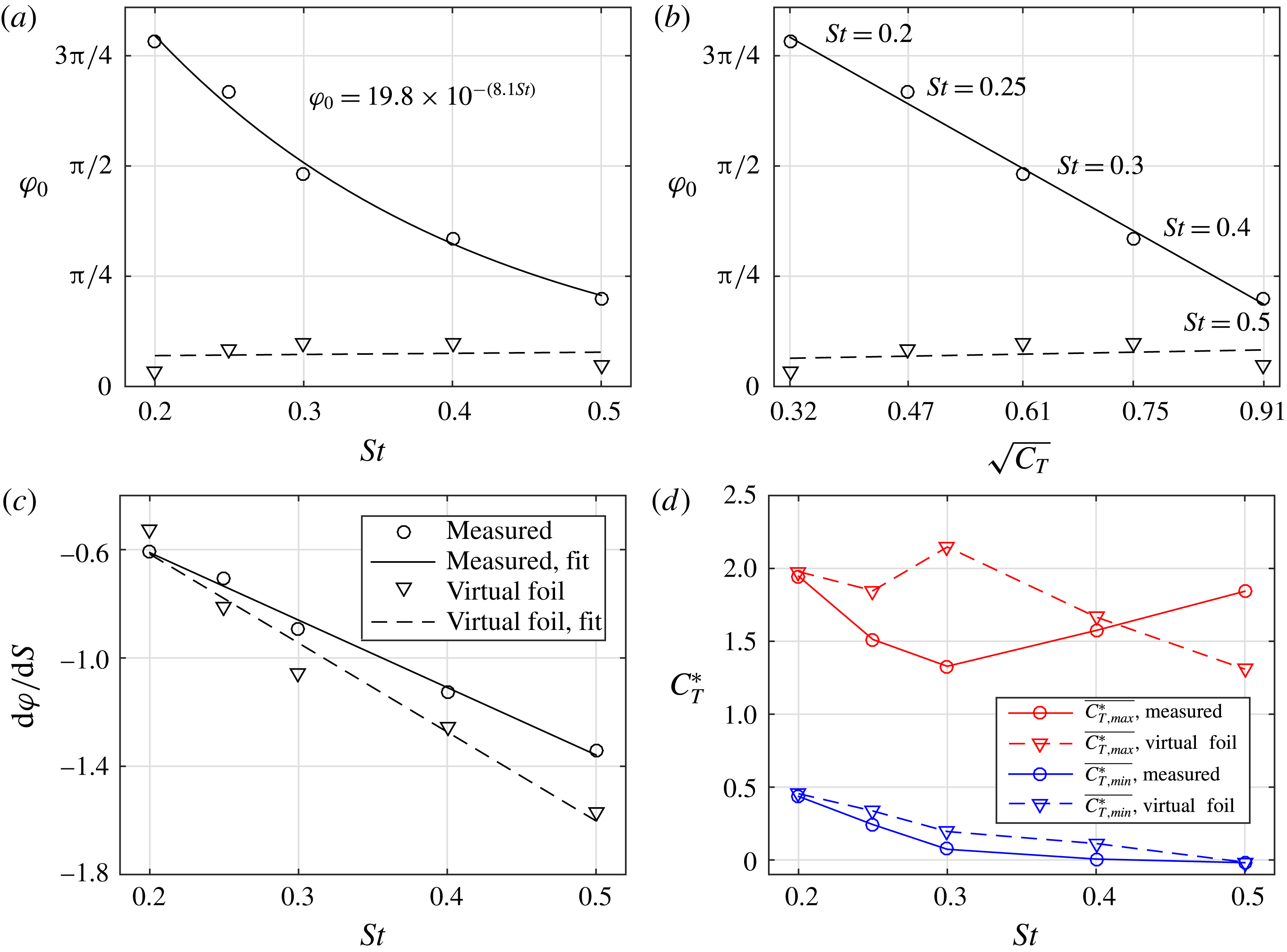
Figure 11. Characteristic values of contour plots for measured and virtual foil data: (a) intercept
 $\unicode[STIX]{x1D711}_{0}$
against St, (b) intercept
$\unicode[STIX]{x1D711}_{0}$
against St, (b) intercept
 $\unicode[STIX]{x1D711}_{0}$
against
$\unicode[STIX]{x1D711}_{0}$
against
 $\sqrt{C_{T}}$
, (c) slope
$\sqrt{C_{T}}$
, (c) slope
 $\text{d}\unicode[STIX]{x1D711}/\text{d}S$
against St, (d) minima
$\text{d}\unicode[STIX]{x1D711}/\text{d}S$
against St, (d) minima
 $\overline{C_{T,min}^{\ast }}$
and maxima
$\overline{C_{T,min}^{\ast }}$
and maxima
 $\overline{C_{T,max}^{\ast }}$
against St. Measured data (calculated using figure 2 and represented by circles) and virtual foil method data (calculated from figure 8 and represented by triangles). Lines are solid for measured data and dashed for virtual foil method.
$\overline{C_{T,max}^{\ast }}$
against St. Measured data (calculated using figure 2 and represented by circles) and virtual foil method data (calculated from figure 8 and represented by triangles). Lines are solid for measured data and dashed for virtual foil method.
A more meaningful metric with which to compare the intercept is the characteristic velocity in the wake of the fore foil. Intuitively, the phase offset that is observed can be interpreted as the time taken for the vortices shed by the fore foil to ‘interact’ with the hind foil including the time taken by the vortices to reach the hind foil and advect past it. Given that the vortices shed by the fore foil have a range of sizes and strengths, it might not be feasible in every case to explicitly measure the time taken for this interaction. Therefore, a proxy for this advection speed is necessary. The square root of the thrust coefficient (
 $\sqrt{C_{T}}$
) is used as it represents the characteristic velocity of the jet in the wake of a thrust-producing foil. Figure 11(b) shows that
$\sqrt{C_{T}}$
) is used as it represents the characteristic velocity of the jet in the wake of a thrust-producing foil. Figure 11(b) shows that
 $\unicode[STIX]{x1D711}_{0}$
is linear with
$\unicode[STIX]{x1D711}_{0}$
is linear with
 $\sqrt{C_{T}}$
, as
$\sqrt{C_{T}}$
, as
 $\unicode[STIX]{x1D711}_{0}$
reduces with increasing value of the thrust of the fore foil. Therefore, as the velocity of the jet in the wake of the fore foil increases (with increasing thrust), the advection speed of the vortices increases and hence the time taken for these vortices to interact with the hind foil reduces. Although the virtual foil method is unable to predict the intercept of the contour bands accurately, the linear relationship of the measured results can be used to determine the necessary phase shift with which to adjust the results from the virtual foil method.
$\unicode[STIX]{x1D711}_{0}$
reduces with increasing value of the thrust of the fore foil. Therefore, as the velocity of the jet in the wake of the fore foil increases (with increasing thrust), the advection speed of the vortices increases and hence the time taken for these vortices to interact with the hind foil reduces. Although the virtual foil method is unable to predict the intercept of the contour bands accurately, the linear relationship of the measured results can be used to determine the necessary phase shift with which to adjust the results from the virtual foil method.
The slope of the thrust coefficient contour bands (
 $\text{d}\unicode[STIX]{x1D711}/\text{d}S$
) is the change in phase (
$\text{d}\unicode[STIX]{x1D711}/\text{d}S$
) is the change in phase (
 $\text{d}\unicode[STIX]{x1D711}$
) over a given change in spacing (
$\text{d}\unicode[STIX]{x1D711}$
) over a given change in spacing (
 $\text{d}S$
) (figure 10) and is a measure of the relative importance of the phase with respect to spacing. The value of
$\text{d}S$
) (figure 10) and is a measure of the relative importance of the phase with respect to spacing. The value of
 $\text{d}S$
is the primary component which determines the slope of the contours, as it represents the characteristic advective wake speed of the vortices generated by the fore foil. Figure 11(c) plots the slope of the contour bands for all Strouhal numbers for both the measured and virtual foil results. There is good agreement between the measured data and the virtual foil results, showing that the virtual foil method is able to predict the slope of the contour bands well. The slope of the contours becomes steeper with increasing Strouhal number, and this trend is linear over the current Strouhal number range. This means that at higher Strouhal numbers, the wake speed is faster, so the hind foil interacts with more vortices in a certain time interval. This is consistent with the interpretation of the phase offset discussed previously.
$\text{d}S$
is the primary component which determines the slope of the contours, as it represents the characteristic advective wake speed of the vortices generated by the fore foil. Figure 11(c) plots the slope of the contour bands for all Strouhal numbers for both the measured and virtual foil results. There is good agreement between the measured data and the virtual foil results, showing that the virtual foil method is able to predict the slope of the contour bands well. The slope of the contours becomes steeper with increasing Strouhal number, and this trend is linear over the current Strouhal number range. This means that at higher Strouhal numbers, the wake speed is faster, so the hind foil interacts with more vortices in a certain time interval. This is consistent with the interpretation of the phase offset discussed previously.
The mean value of the high thrust contour is calculated by taking the average of the maximum thrust coefficient for each spacing, and the minimum is determined in a corresponding fashion. The minimum thrust decreases with Strouhal number, showing that the detrimental foil–vortex interactions are stronger at higher frequencies. This trend is captured well with the virtual foil method. However, the virtual foil method overestimates the maximum thrust for most frequencies (figure 11
d), which can be explained by examining the efficiency of the single foil. Figure 14(b) shows that the efficiency of the single foil increases sharply up to the maximum at
 $St=0.3$
, after which it decreases more slowly. This is the inverse trend of the maximum thrust coefficient for the measured results of figure 11(d) and shows that when the single foil has a high efficiency, the maximum thrust augmentation of the hind foil is lower. We propose that this is because when the foil is flapping with kinematics that give it a high efficiency, it is already operating close to its maximum efficiency, so further increases in thrust are proportionally harder to obtain.
$St=0.3$
, after which it decreases more slowly. This is the inverse trend of the maximum thrust coefficient for the measured results of figure 11(d) and shows that when the single foil has a high efficiency, the maximum thrust augmentation of the hind foil is lower. We propose that this is because when the foil is flapping with kinematics that give it a high efficiency, it is already operating close to its maximum efficiency, so further increases in thrust are proportionally harder to obtain.
Knowledge of the slopes, intercepts, maxima and minima of the phase–spacing contour plots over a range of frequencies is powerful for the design of tandem flapping foil propulsors as it allows prediction of the parametric combinations that lead to high thrust without measurements of the entire parameter space. The contour plot of any Strouhal number between the frequencies given here can be reconstructed by using the slope and offset values given in figures 11(c) and 11(b).
For the three lowest Strouhal numbers (figure 9 (
 $St=0.25$
not shown)), the virtual foil method predicts the form of the efficiency contours, but overpredicts the efficiency over the whole phase–spacing range. For certain phase–spacing combinations for the highest two Strouhal numbers, the virtual foil method calculates a power close to zero, and therefore predicts efficiency values that unrealistically low or high. We consider these errors to be because the virtual foil method does not account for additional losses in the flow due to the hind foil, and more work is required to understand this fully.
$St=0.25$
not shown)), the virtual foil method predicts the form of the efficiency contours, but overpredicts the efficiency over the whole phase–spacing range. For certain phase–spacing combinations for the highest two Strouhal numbers, the virtual foil method calculates a power close to zero, and therefore predicts efficiency values that unrealistically low or high. We consider these errors to be because the virtual foil method does not account for additional losses in the flow due to the hind foil, and more work is required to understand this fully.
The virtual foil method not only leads to insights regarding the mechanism of the thrust augmentation of tandem flapping foils, and about the upstream inflow condition of immersed bodies, but it also greatly reduces the number of experiments required to investigate the time-averaged thrust over the entire spacing–phase–frequency parameter space of tandem flapping foils. This method shows that instead of running a tandem case of every combination of these parameters, just one run of a single foil is all that is required to predict the performance augmentation.
4 Conclusions and outlook
Two-dimensional numerical simulations revealed that the thrust production of the hind foil can be as much as twice the value of a single foil. For the first time, this effect is shown to occur over a range of Strouhal numbers. This extra thrust would be extremely advantageous for a propulsion system, but the benefit is observed only for certain parameter combinations. Analysis of instantaneous velocity and vorticity fields revealed that the high-performance and low-performance cases had the same type of foil–vortex interaction, regardless of the particular phase, spacing and frequency at which these cases occurred. When the hind foil weaves between the incoming vortices, it has high performance, but when it intercepts the vortices, the hind foil has low performance.
A simple virtual foil method that uses the instantaneous velocity field of a single flapping foil showed that the dominant parameter affecting the performance augmentation is the modification of the angle of attack of the hind foil due to the incoming vortex street. The virtual foil method was used to predict the thrust and efficiency of the hind foil over the entire phase–spacing–frequency space and was able to capture the key features of the performance augmentation.
The thrust coefficient contour bands were characterised through the use of four quantities: the intercept (
 $\unicode[STIX]{x1D711}_{0}$
), slope (
$\unicode[STIX]{x1D711}_{0}$
), slope (
 $\text{d}\unicode[STIX]{x1D711}/\text{d}S$
), average maximum and average minimum. The intercept of the bands was observed to vary linearly with the characteristic vortex advection velocity of the wake of the fore foil, represented by the square root of the thrust coefficient. This feature was not captured by the virtual foil method as it cannot account for the inherent time delay in the flow necessary for the advecting vortices to influence the hydrodynamics of the hind foil. The slope of the contour bands was shown to vary linearly over the range of Strouhal numbers considered, which was captured accurately by the virtual foil method. The maximum value of the contour bands was shown to be related to the efficiency of the fore foil: a high efficiency of the single foil leads to a lower thrust augmentation, and this is because the fore foil is already operating close to its maximum effectiveness, so it is harder to achieve further increases in thrust. The minimum value of the bands was seen to decrease with Strouhal number, implying stronger detrimental interactions between the foil and incoming vortices with increasing frequency, which was captured well by the virtual foil model.
$\text{d}\unicode[STIX]{x1D711}/\text{d}S$
), average maximum and average minimum. The intercept of the bands was observed to vary linearly with the characteristic vortex advection velocity of the wake of the fore foil, represented by the square root of the thrust coefficient. This feature was not captured by the virtual foil method as it cannot account for the inherent time delay in the flow necessary for the advecting vortices to influence the hydrodynamics of the hind foil. The slope of the contour bands was shown to vary linearly over the range of Strouhal numbers considered, which was captured accurately by the virtual foil method. The maximum value of the contour bands was shown to be related to the efficiency of the fore foil: a high efficiency of the single foil leads to a lower thrust augmentation, and this is because the fore foil is already operating close to its maximum effectiveness, so it is harder to achieve further increases in thrust. The minimum value of the bands was seen to decrease with Strouhal number, implying stronger detrimental interactions between the foil and incoming vortices with increasing frequency, which was captured well by the virtual foil model.
A summary of the virtual foil method and necessary corrections are as follows: (i) perform a simulation or experiment of a single foil and record the instantaneous velocity field at every time throughout the flapping cycle; (ii) for each time step use the velocity field along with the heave and pitch positions and velocities of a virtual hind foil for a particular phase and spacing combination to determine the instantaneous angle of attack and induced velocity magnitude of the virtual hind foil; (iii) use the instantaneous angle of attack and induced velocity magnitude to calculate the instantaneous lift, drag and moment of the foil by using steady-state lift, drag and moment equations, the coefficients of which can be found using steady-state simulations, experiments or panel methods; (iv) use these to calculate the thrust and efficiency of the virtual hind foil; (v) repeat steps 2–4 for a range of phases and spacings to produce a contour plot for that frequency; (vi) adjust this contour plot in phase by using the values of
 $\unicode[STIX]{x1D711}_{0}$
given in figure 11(b); (vii) use this new contour plot to determine the set of phase–spacing combinations that yield high thrust for that frequency.
$\unicode[STIX]{x1D711}_{0}$
given in figure 11(b); (vii) use this new contour plot to determine the set of phase–spacing combinations that yield high thrust for that frequency.
Finally, it should be noted that this study has focused on specific kinematics that involve both pitch and heave, with a given phase difference between the oscillations about the two axes. Further simulations or experiments involving pure pitch and pure heave cases would be valuable to determine whether the observations as well as the virtual foil model presented in this study could extend to other types of kinematics.
Acknowledgements
We gratefully acknowledge the funding from EPSRC, Ginko investements Ltd and the Leverhulme Trust.
Supplementary movies
Supplementary movies are available at https://doi.org/10.1017/jfm.2017.457.
Appendix A. Optimisation of single foil kinematics
To ensure that the foils have the most efficient kinematics over a range of frequencies, a preliminary study was conducted to determine the optimum maximum angle of attack. This was achieved by performing computations of single foils at three Strouhal numbers (0.2, 0.3 and 0.4), and 19 maximum pitch angles (
 $0^{\circ }$
–
$0^{\circ }$
–
 $45^{\circ }$
in steps of
$45^{\circ }$
in steps of
 $2.5^{\circ }$
). Figure 12(a) shows that the peaks in propulsive efficiency occur at different values of the maximum pitch angle,
$2.5^{\circ }$
). Figure 12(a) shows that the peaks in propulsive efficiency occur at different values of the maximum pitch angle,
 $\unicode[STIX]{x1D703}_{max}$
. When plotted against maximum angle of attack however, these peaks collapse to give maximum efficiencies for (
$\unicode[STIX]{x1D703}_{max}$
. When plotted against maximum angle of attack however, these peaks collapse to give maximum efficiencies for (
 $5^{\circ }<\unicode[STIX]{x1D6FC}_{max}<10^{\circ }$
). Maximum angles of attack of
$5^{\circ }<\unicode[STIX]{x1D6FC}_{max}<10^{\circ }$
). Maximum angles of attack of
 $10^{\circ }$
were therefore chosen for all the simulations presented in the current study to ensure that the tandem-foil results were within the high-efficiency regime.
$10^{\circ }$
were therefore chosen for all the simulations presented in the current study to ensure that the tandem-foil results were within the high-efficiency regime.

Figure 12. Propulsive efficiency (
 $\unicode[STIX]{x1D702}$
) against maximum pitch angle (
$\unicode[STIX]{x1D702}$
) against maximum pitch angle (
 $\unicode[STIX]{x1D703}_{max}$
) and maximum angle of attack (
$\unicode[STIX]{x1D703}_{max}$
) and maximum angle of attack (
 $\unicode[STIX]{x1D6FC}_{max}$
) for three Strouhal numbers:
$\unicode[STIX]{x1D6FC}_{max}$
) for three Strouhal numbers:
 $St=0.2$
(green, dashed line),
$St=0.2$
(green, dashed line),
 $St=0.3$
(blue, dotted line),
$St=0.3$
(blue, dotted line),
 $St=0.4$
(black, solid line).
$St=0.4$
(black, solid line).

Figure 13. Percentage change in thrust ratio (
 $dC_{T}^{\ast }(\%)$
) for simulations of various resolutions (
$dC_{T}^{\ast }(\%)$
) for simulations of various resolutions (
 $r$
) compared to the case of resolution of 128 grid points per chord. Dotted curve is fitted exponential.
$r$
) compared to the case of resolution of 128 grid points per chord. Dotted curve is fitted exponential.

Figure 14. Comparisons of the thrust predicted using the virtual foil method to the measured thrust for a single foil. (a) Mean thrust coefficients for measured (solid line) and virtual foil (dashed line) results for all
 $St$
, (b) efficiency of single foil for measured (solid line) and virtual foil (dashed line) results for all
$St$
, (b) efficiency of single foil for measured (solid line) and virtual foil (dashed line) results for all
 $St$
, (c) measured thrust (solid line) and estimated thrust (dashed line) coefficient histories for
$St$
, (c) measured thrust (solid line) and estimated thrust (dashed line) coefficient histories for
 $St=0.2$
, (d) measured thrust (solid line) and estimated thrust (dashed line) coefficient histories for
$St=0.2$
, (d) measured thrust (solid line) and estimated thrust (dashed line) coefficient histories for
 $St=0.4$
, (e) mean power coefficient
$St=0.4$
, (e) mean power coefficient
 $\overline{C_{P}}$
for all
$\overline{C_{P}}$
for all
 $St$
, (f) the side force coefficient
$St$
, (f) the side force coefficient
 $C_{S}$
for
$C_{S}$
for
 $St=0.4$
.
$St=0.4$
.
Appendix B. Resolution sensitivity analysis
To determine the sensitivity of the solutions to the computational resolution, a set of simulations with various resolutions, all for
 $St=0.2$
and
$St=0.2$
and
 $\unicode[STIX]{x1D711}=\unicode[STIX]{x03C0}/2$
, were performed. Figure 13 shows the percentage change in thrust ratio (
$\unicode[STIX]{x1D711}=\unicode[STIX]{x03C0}/2$
, were performed. Figure 13 shows the percentage change in thrust ratio (
 $dC_{T}^{\ast }(\%)$
) for all resolutions (
$dC_{T}^{\ast }(\%)$
) for all resolutions (
 $r$
) compared to a resolution of 128. The
$r$
) compared to a resolution of 128. The
 $r=64$
case has a value within 4 % of the
$r=64$
case has a value within 4 % of the
 $r=128$
case, and is only marginally higher than the
$r=128$
case, and is only marginally higher than the
 $r=96$
case, showing that a resolution of 64 gives a suitable accuracy with the lowest computational expense.
$r=96$
case, showing that a resolution of 64 gives a suitable accuracy with the lowest computational expense.
Appendix C. Virtual foil method applied to single foil
To determine the suitability of the virtual foil method to predict the forces of the hind foil in a tandem-foil system, the method must first be checked for the case of a single foil.
Figure 14(a) shows that the virtual foil method overestimates the mean thrust of the hind foil for low frequencies and underestimates it for high frequencies. For lower frequencies the shape of the force history is well produced, although the magnitude is overestimated during the entire flapping cycle (figure 14
c), leading to the higher mean. For the higher frequencies the shape of the force histories for the measured and virtual foil results are markedly different (figure 14
d), but the overall average is very similar. The differences in shape are due to stronger dynamic effects that occur at higher frequencies. The discrepancies can be characterised as those that overestimate the thrust (when
 $0<\unicode[STIX]{x1D70F}<0.25$
and
$0<\unicode[STIX]{x1D70F}<0.25$
and
 $0.5<\unicode[STIX]{x1D70F}<0.75$
) and those that underestimate the thrust (when
$0.5<\unicode[STIX]{x1D70F}<0.75$
) and those that underestimate the thrust (when
 $0.25<\unicode[STIX]{x1D70F}<0.5$
and
$0.25<\unicode[STIX]{x1D70F}<0.5$
and
 $0.75<\unicode[STIX]{x1D70F}<1.0$
). The underestimation of the thrust occurs because the virtual foil method predicts a sharp rise in thrust as soon as the foil starts moving downwards (at
$0.75<\unicode[STIX]{x1D70F}<1.0$
). The underestimation of the thrust occurs because the virtual foil method predicts a sharp rise in thrust as soon as the foil starts moving downwards (at
 $\unicode[STIX]{x1D70F}=0.25$
), whereas the measured results show a low pressure region on the surface of the foil, which convects down the chord before it is shed, producing drag during this time interval. The overestimation of the thrust occurs because a leading edge vortex is produced as the foil is moving up or down, which increases in strength before being shed at the extremes of the flap. This dynamic vortex effect is not captured by the virtual foil method, which predicts a near-constant thrust for the majority of the stroke (
$\unicode[STIX]{x1D70F}=0.25$
), whereas the measured results show a low pressure region on the surface of the foil, which convects down the chord before it is shed, producing drag during this time interval. The overestimation of the thrust occurs because a leading edge vortex is produced as the foil is moving up or down, which increases in strength before being shed at the extremes of the flap. This dynamic vortex effect is not captured by the virtual foil method, which predicts a near-constant thrust for the majority of the stroke (
 $0.4<\unicode[STIX]{x1D70F}<0.6$
).
$0.4<\unicode[STIX]{x1D70F}<0.6$
).
The virtual foil method overestimates the efficiency by around
 $40\,\%$
. For low frequencies this is primarily due to overestimation of the thrust (figure 14
a), and for high frequencies this is primarily due to overestimation of the power (figure 14
e) through overestimation of the heave force during the flapping cycle (figure 14
f).
$40\,\%$
. For low frequencies this is primarily due to overestimation of the thrust (figure 14
a), and for high frequencies this is primarily due to overestimation of the power (figure 14
e) through overestimation of the heave force during the flapping cycle (figure 14
f).
Despite its inability to capture all the intricacies of the force production of a flapping foil, the virtual foil method predicts the mean thrust coefficient well and is therefore deemed suitable for the analysis of tandem flapping foils.


