


1. Introduction
Microorganisms inhabit the Earth in a vast variety of environments (Omori et al. Reference Omori, Habe, Yoshida, Horinouchi, Saiki and Nojiri2003). Some of these microorganisms respond to outside stimuli and move in selected directions. These responses are called taxis. Taxis responding to gravity, light and chemicals are respectively called gravitaxis, phototaxis and chemotaxis. In suspension, when a certain quantity of microorganisms accumulates near a free surface due to taxis, cells of the microorganisms fall, thus bioconvection is generated (Platt Reference Platt1961) because the cells are denser than water (Hart & Edwards Reference Hart and Edwards1987).
Many studies have been made on bioconvection (Pedley & Kessler Reference Pedley and Kessler1992; Hillesdon, Pedley & Kessler Reference Hillesdon, Pedley and Kessler1995; Hillesdon & Pedley Reference Hillesdon and Pedley1996; Bees & Hill Reference Bees and Hill1997; Metcalfe & Pedley Reference Metcalfe and Pedley1998, Reference Metcalfe and Pedley2001; Czirók, Jánosi & Kessler Reference Czirók, Jánosi and Kessler2000; Ghorai & Hill Reference Ghorai and Hill2002; Yanaoka, Inamura & Suzuki Reference Yanaoka, Inamura and Suzuki2007, Reference Yanaoka, Inamura and Suzuki2008; Williams & Bees Reference Williams and Bees2011; Chertock et al. Reference Chertock, Fellner, Kurganov, Lorz and Markowich2012; Kage et al. Reference Kage, Hosoya, Baba and Mogami2013; Karimi & Paul Reference Karimi and Paul2013). Microorganisms have been used for environmental cleanup in various fields (Omori et al. Reference Omori, Nojiri, Horinouchi and Kasuga2002, Reference Omori, Habe, Yoshida, Horinouchi, Saiki and Nojiri2003; Hirooka & Nagase Reference Hirooka and Nagase2003). Bioconvection can be applied to driving micromechanical systems (Itoh, Toida & Saotome Reference Itoh, Toida and Saotome2001, Reference Itoh, Toida and Saotome2006), mixing chemicals (Geng & Kuznetsov Reference Geng and Kuznetsov2005), detecting toxicity (Noever & Matsos Reference Noever and Matsos1991a,Reference Noever and Matsosb; Noever, Matsos & Looger Reference Noever, Matsos and Looger1992) and controlling microorganisms in biochips, as well as other applications. Furthermore, the production of biofuels by microorganisms has attracted attention from the viewpoint of being clean and environmentally friendly. Bees & Croze (Reference Bees and Croze2014) discussed the possibility that microorganisms with taxis may be able to mix biofuel-producing microorganisms efficiently. Therefore, for the efficient utilization of microorganisms in various fields, it is important to determine the behaviour of microorganisms and the mass transfer characteristics in bioconvection generated by microorganisms with taxis.
Regarding bioconvection generated by chemotactic bacteria responding to oxygen, theoretical (Hillesdon & Pedley Reference Hillesdon and Pedley1996; Metcalfe & Pedley Reference Metcalfe and Pedley1998, Reference Metcalfe and Pedley2001), experimental (Pedley & Kessler Reference Pedley and Kessler1992; Hillesdon et al. Reference Hillesdon, Pedley and Kessler1995; Czirók et al. Reference Czirók, Jánosi and Kessler2000) and numerical (Yanaoka et al. Reference Yanaoka, Inamura and Suzuki2007, Reference Yanaoka, Inamura and Suzuki2008; Chertock et al. Reference Chertock, Fellner, Kurganov, Lorz and Markowich2012; Lee & Kim Reference Lee and Kim2015) studies have been conducted. However, earlier numerical studies were two-dimensional or three-dimensional analyses on a single plume with a fixed wavelength (Yanaoka et al. Reference Yanaoka, Inamura and Suzuki2007, Reference Yanaoka, Inamura and Suzuki2008). Hence it was not possible to capture complicated three-dimensional phenomena that multiple plumes exhibit in the chamber. Although basic studies on the wavelength of bioconvection patterns have been carried out (Bees & Hill Reference Bees and Hill1997; Czirók et al. Reference Czirók, Jánosi and Kessler2000; Ghorai & Hill Reference Ghorai and Hill2002; Karimi & Paul Reference Karimi and Paul2013), no studies have been reported on the influences of wavelength variations on the transport characteristics and interference between plumes.
Studies on the control of bioconvection have been performed to utilize microorganisms for engineering purposes (Itoh et al. Reference Itoh, Toida and Saotome2001, Reference Itoh, Toida and Saotome2006; Kuznetsov Reference Kuznetsov2005). Furthermore, various studies have been conducted on nano-bioconvection in suspensions containing nanoparticles and bacteria (Geng & Kuznetsov Reference Geng and Kuznetsov2005; Kuznetsov Reference Kuznetsov2011; Uddin, Kabir & Bég Reference Uddin, Kabir and Bég2016; Zadeha et al. Reference Zadeha, Mehryanb, Sheremetc, Izadid and Ghodrate2020). Recently, bioconvection in suspensions containing microorganisms and nanoparticles under an applied magnetic field has been investigated (Naseem et al. Reference Naseem, Shafiq, Zhao and Naseem2017; Khan et al. Reference Khan, Salahuddin, Malik, Alqarni and Alqahtani2020; Shi et al. Reference Shi, Hamid, Khan, Kumar, Gowda, Prasannakumara, Shah, Khan and Chung2021). New applicative research on bioconvection is underway. However, in the previous studies, the phenomenon of three-dimensional bioconvection has not been captured because a stability analysis was performed or the fundamental equations were solved by similarity transformation. Bioconvection with multiple microbial plumes is complex, and the details of the transport characteristics in bioconvection have not been clarified.
Bioconvection is a three-dimensional phenomenon, and multiple plumes will exist in a chamber. Under such circumstances, the plumes interfere with each other, and the accompanying change in the wavelength of the bioconvection pattern affects the transport characteristics. From the above viewpoints, we simulate three-dimensional bioconvection generated by oxygen-reactive chemotactic bacteria, then clarify the bioconvection patterns, interference between plumes, the wavelengths of each pattern, and the transport characteristics of cells and oxygen when multiple plumes arise.
2. Numerical procedures
Figure 1 shows the flow configuration and coordinate system. A suspension in a chamber contains bacterial cells, and the depth of the suspension is  $h$. The origin is at the bottom wall of the chamber. The
  $x$- and
  $y$-axes are in the horizontal and vertical directions, respectively, and the
  $z$-axis is in the direction perpendicular to the page.

Figure 1. Flow configuration and coordinate system.
We assume that the suspension is sufficiently dilute for hydrodynamic cell–cell interactions to be negligible, and consider an incompressible viscous fluid. The fundamental equations are the continuity equation, the momentum equation under the Boussinesq approximation, and the conservation equations for cells and oxygen (Hillesdon et al. Reference Hillesdon, Pedley and Kessler1995; Hillesdon & Pedley Reference Hillesdon and Pedley1996), given as
 $$\begin{gather} \boldsymbol{\nabla} \boldsymbol{\cdot} {\boldsymbol{u}}=0, \end{gather}$$
 $$\begin{gather}\frac{\partial {\boldsymbol{u}}}{\partial t} + \boldsymbol{\nabla} \boldsymbol{\cdot} ({\boldsymbol{u}} \otimes {\boldsymbol{u}}) ={-} \frac{1}{\rho}\,\boldsymbol{\nabla} p + \nu\,\nabla^{2} {\boldsymbol{u}} + \frac{g n V (\rho_n - \rho) {\boldsymbol{e}}}{\rho}, \end{gather}$$
 $$\begin{gather}\frac{\partial n}{\partial t} + \boldsymbol{\nabla} \boldsymbol{\cdot} ({\boldsymbol{u}} n + {\boldsymbol{V}} n - {\boldsymbol{D}}_n\,\boldsymbol{\nabla} n) = 0, \end{gather}$$
 $$\begin{gather}\frac{\partial c}{\partial t} + \boldsymbol{\nabla} \boldsymbol{\cdot} ({\boldsymbol{u}} c - D_c\,\boldsymbol{\nabla} c) ={-} K n, \end{gather}$$
where  $t$ is time,
  ${\boldsymbol {u}}$ is flow velocity,
  $p$ is pressure,
  $\rho$ and
  $\nu$ are the density and kinematic viscosity of the fluid, respectively,
  $\rho _n$ is the density of the cell,
  $V$ is the volume of the cell,
  $g$ is the gravity acceleration,
  ${\boldsymbol {e}}=-\hat {\boldsymbol {y}}$ is the unit vector in the direction of gravity,
  $n$ is cell concentration,
  $c$ is oxygen concentration,
  ${\boldsymbol {V}}$ is the average cell swimming velocity,
  ${\boldsymbol {D}}_n$ is the cell diffusivity tensor,
  $D_c$ is the oxygen diffusivity, and
  $K$ is the rate of oxygen consumption by cells.
In this study, the swimming of microorganisms is modelled similarly to that of Hillesdon et al. (Reference Hillesdon, Pedley and Kessler1995). Berg & Brown (Reference Berg and Brown1972) found that the swimming velocity of microorganisms has both directional and random components. The random swimming of the cell is modelled as cell diffusion. The cell diffusion is assumed to be isotropic, and the cell diffusivity tensor  ${\boldsymbol {D}}_n$ is modelled as
  ${\boldsymbol {D}}_n=D_{n0}\, H(c^*)\,{\boldsymbol {I}}$. Here,
  $c^*$ is the non-dimensional oxygen concentration,
  $H(c^*)$ is a step function, and
  ${\boldsymbol {I}}$ is the identity tensor. This
  $c^*$ is defined as
  $c^*=(c-c_{min})/(c_0-c_{min})$, where
  $c_0$ is the initial oxygen concentration, and
  $c_{min}$ is the minimum oxygen concentration required for the cell to be active. Next, the directional swimming of the cell is modelled as an average swimming velocity. The average cell swimming velocity vector
  ${\boldsymbol {V}}$ is modelled as being proportional to the oxygen concentration gradient and is defined as
  ${\boldsymbol {V}}=b V_s\,H(c^*)\,\boldsymbol {\nabla } c^*$. The oxygen consumption rate
  $K$ by cells is modelled as
  $K=K_0 H(c^*)$, like that of Hillesdon et al. (Reference Hillesdon, Pedley and Kessler1995). Here,
  $D_{n0}$,
  $b$,
$b$,  $V_s$ and
  $K_0$ are constants. In this study,
  $H(c^*)$ is modelled with an approximate equation
  $H(c^*)=1-\exp (-c^*/c^*_1)$, to suppress discontinuous changes due to the step function (Hillesdon et al. Reference Hillesdon, Pedley and Kessler1995). Also,
  $c^*_1$ is 0.01 (Hillesdon et al. Reference Hillesdon, Pedley and Kessler1995; Yanaoka et al. Reference Yanaoka, Inamura and Suzuki2007, Reference Yanaoka, Inamura and Suzuki2008). Hillesdon et al. (Reference Hillesdon, Pedley and Kessler1995) investigated the effect of
  $c_1^*$ on the concentration distribution in a stationary field, and the qualitative trend did not change. In the present study,
  $c_1^*$ is set to a small value. Therefore, in a shallow chamber treated in the present study, since oxygen is transported to the bottom, the step function
  $H(c^*)$ is approximately 1.0, and the modelling of
  $H(c^*)$ does not affect the calculation results.
A non-slip boundary condition is set at the bottom wall, and the gradients perpendicular to the wall are to be assumed zero for the cell and oxygen concentrations. At the free surface, a slip boundary condition is imposed for the velocity field, the flux of cell concentration is zero, and the oxygen concentration is constant. Further, periodic boundary conditions are imposed in the  $x$- and
  $z$-directions for the velocity and concentration fields.
The variables of the fundamental equations are non-dimensionalized in the same way as in previous studies (Hillesdon et al. Reference Hillesdon, Pedley and Kessler1995; Yanaoka et al. Reference Yanaoka, Inamura and Suzuki2007, Reference Yanaoka, Inamura and Suzuki2008) as follows:
 \begin{equation} \boldsymbol{x}^* = \frac{\boldsymbol{x}}{h}, \quad \boldsymbol{u}^* = \frac{\boldsymbol{u}}{D_{n0}/h}, \quad p^* = \frac{p}{\rho (D_{n0}/h)^2}, \quad t^* = \frac{t}{h^2/D_{n0}}, \quad n^* = \frac{n}{n_0}, \end{equation}
where the superscript  $*$ represents a non-dimensional variable, and
  $n_0$ is the initial cell concentration. Thus the non-dimensional fundamental equations are written as
 $$\begin{gather} \boldsymbol{\nabla} \boldsymbol{\cdot} \boldsymbol{u}^* = 0, \end{gather}$$
 $$\begin{gather}\frac{1}{Sc} \left[ \frac{\partial \boldsymbol{u}^*}{\partial t^*} + \boldsymbol{\nabla} \boldsymbol{\cdot} (\boldsymbol{u}^* \otimes \boldsymbol{u}^*) \right] ={-} \boldsymbol{\nabla} p^* + \nabla^{2} \boldsymbol{u}^* + Ra\,n^* \boldsymbol{e}, \end{gather}$$
 $$\begin{gather}\frac{\partial n^*}{\partial t^*} + \boldsymbol{\nabla} \boldsymbol{\cdot} \left[\boldsymbol{u}^* n^* + H(c^*)\,\gamma n^*\,\boldsymbol{\nabla} c^* - H(c^*)\,\boldsymbol{\nabla} n^*\right] = 0, \end{gather}$$
 $$\begin{gather}\frac{\partial c^*}{\partial t^*} + \boldsymbol{\nabla} \boldsymbol{\cdot} (\boldsymbol{u}^* c^* - \delta\,\boldsymbol{\nabla} c^*) ={-} H(c^*)\,\delta \beta n^*, \end{gather}$$
where the non-dimensional parameters are given by (2.10a–e) below. The parameter  $\beta$ represents the strength of oxygen consumption relative to its diffusion,
  $\gamma$ is a measure of the relative strengths of directional and random swimming, and
  $\delta$ is the ratio of oxygen diffusivity to cell diffusivity. Also,
  $Ra$ is the Rayleigh number, and
  $Sc$ is the Schmidt number. We have
 \begin{align} \beta = \frac{K_0 n_0 h^2}{D_c (c_0 - c_{{min}})}, \quad \gamma = \frac{b V_s}{D_{n0}}, \quad \delta = \frac{D_c}{D_{n0}}, \quad Ra = \frac{V n_0 g h^3 (\rho_n - \rho)}{\nu D_{n0} \rho}, \quad Sc = \frac{\nu}{D_{n0}} . \end{align}
The governing equations are solved using the SMAC method (Amsden & Harlow Reference Amsden and Harlow1970). This study uses the Euler implicit method for the time differentials, and the second-order central difference scheme for the space differentials.
3. Calculation conditions
This study considers chemotactic bacteria responding to oxygen as microorganisms with taxis, and investigates the characteristics of three-dimensional bioconvection in the chamber. As the initial condition, the suspension is stationary, and the cell and oxygen concentrations are constant. Similar to the previous study (Ghorai & Hill Reference Ghorai and Hill2002), low initial disturbances are added to the cell concentration in the suspension to model the initial state in an experiment of bioconvection. The initial concentration is defined as
 \begin{equation} n = n_0 \left[ 1 + \varepsilon\,A(x,y) \right], \end{equation}
where  $\varepsilon =10^{-2}$, and
  $A(x,y)$ is a random number generated in the range
  $-1$ to 1. The random number is generated by the Mersenne twister method (Matsumoto & Nishimura Reference Matsumoto and Nishimura1998), and the initial value is given by the linear congruent method. To investigate the stability of bioconvection with respect to disturbance, we use the obtained calculation result as an initial condition.
The  $x$- and
  $z$-dimensions of the computational region are set to
  $10h$. To clarify the effect of the length of the calculation area on the formation of bioconvection, we also performed a calculation for the calculation area
  $L=20h$. This study used four uniform grids,
  $91 \times 31 \times 91$ (grid1),
  $101 \times 51 \times 101$ (grid2),
  $111 \times 81 \times 111$ (grid3) and
  $141 \times 101 \times 141$ (grid4), for
  $L=10h$ to examine the grid dependency of the numerical results. We confirmed that the grid resolution of grid2 was suitable for obtaining valid results, so the results of grid2 are shown in the following. In the calculation for
  $L=20h$, we used a uniform grid
  $201 \times 51 \times 201$, which has the same resolution as grid2.
Non-dimensional parameters are given using the properties of Bacillus subtilis that responds to oxygen gradients. The diffusion coefficient of bacteria  $D_{n0}$ is different in each study, and the range is
  $10^{-6}$ to
  $10^{-5}\ {\rm cm}^2\ {\rm s}^{-1}$ (Hillesdon et al. Reference Hillesdon, Pedley and Kessler1995; Hillesdon & Pedley Reference Hillesdon and Pedley1996; Tuval et al. Reference Tuval, Cisneros, Dombrowski, Wolgemuth, Kessler and Goldstein2005). This study takes
  $D_{n0}=10^{-5}\ {\rm cm}^2\ {\rm s}^{-1}$ and adopts values for the other properties from Hillesdon et al. (Reference Hillesdon, Pedley and Kessler1995) and Hillesdon & Pedley (Reference Hillesdon and Pedley1996). Therefore, the non-dimensional base parameters are
  $\beta =1$,
  $\gamma =2$,
  $\delta =2$ and
  $Sc=1000$. We change some base parameters to investigate the effects of the physical properties of bacteria and oxygen on bioconvection. The calculation was conducted for eight different Rayleigh numbers,
  $Ra=0$, 250, 500, 1000, 2000, 3000, 4000 and 5000. The bioconvection occurs above the critical Rayleigh number. Variations of the bioconvection patterns and the wavelengths depending on the initial condition have been observed in earlier experimental research (Bees & Hill Reference Bees and Hill1997). At
  $Ra=500$ and 5000, greater than the critical Rayleigh number, we have investigated whether the same tendency as the experimental result is observed for ten kinds of initial disturbance to the cell concentration. The results for all Rayleigh numbers are convergent solutions and represent steady-state flow and concentration fields.
4. Numerical results and discussion
4.1. Comparison with the theoretical solution
The present numerical result is compared with the linear theoretical solution (Hillesdon et al. Reference Hillesdon, Pedley and Kessler1995) to confirm its validity. The theoretical value is a solution for a shallow chamber. Figure 2 shows the cell and oxygen concentration distributions in the  $y$-direction for
  $Ra=0$, 250 and 500. Here, the cross-sections are at
  $x/h=5.0$,
  $z/h=5.0$ for
  $Ra=0$ and
  $Ra=250$, and
  $x/h=5.9$,
  $z/h=4.1$ at the centre of the plume for
  $Ra=500$. The plume is shown in figures 4 and 5. We define the plume centre as the position where the cell concentration on the free surface is maximum. These calculation results for
  $Ra=0, 250$ agree well with the theoretical solution. However, it is confirmed that a large difference appears between the result at
  $Ra=500$ and the theoretical result, suggesting the occurrence of bioconvection, which is a nonlinear phenomenon. The previous study (Yanaoka et al. Reference Yanaoka, Inamura and Suzuki2008) showed that bioconvection occurs at a Rayleigh number greater than the critical number. In this study, since bioconvection occurs at
  $Ra=500$, it is considered that the critical Rayleigh number lies between
  $Ra=250$ and
  $Ra=500$.

Figure 2. Comparison of concentration distributions with linear theoretical solution (Hillesdon et al. Reference Hillesdon, Pedley and Kessler1995) for (a) bacteria, and (b) oxygen.
4.2. Occurrence of bioconvection
First, we investigate the occurrence of bioconvection when the Rayleigh number is changed. Figures 3 and 4 show the flow and concentration fields for  $Ra=250, 500$. At
  $Ra=250$, the bacterial cells are concentrated near the water surface because they react with the oxygen supplied from the water surface and move upward due to chemotaxis. As the fluid is almost stationary and is not transported by convection, the oxygen concentration distribution is two-dimensional. The oxygen concentration decreases from the water surface to the lower wall. From above, because the suspension is stable up to
  $Ra=250$ and bioconvection does not occur, it is considered that the critical Rayleigh number is at
  $Ra>250$. In the cell concentration field of
  $Ra=500$ shown in figure 4(a), high-concentration cells concentrated near the water surface settle towards the lower wall at
  $x/h=3.3$. This falling region of cells is called a plume, and this result suggests the occurrence of bioconvection. As shown in figure 4(d), the plumes form in a staggered manner, so the cross-section of
  $z/h=6.5$ is located across one plume. Therefore, in figure 4(a), the influence of one plume appears significantly. Still, even around
  $x/h=7.0$ and 9.5, the cell concentration is distorted by the influence of the surrounding plumes. Slight fluctuations are observed in the oxygen concentration distribution, and weak convection occurs in the velocity vector. In the oxygen concentration field for
  $Ra=500$, because the Rayleigh number is low, the effect of diffusion is greater than that of convection. In the cell concentration field, even if the Rayleigh number is low, transport by directional swimming works in addition to random swimming, so the effect of convection becomes large. Since bacteria consume oxygen, oxygen consumption increases in the plume, where the cell concentration is high. Therefore, the oxygen concentration does not have a distribution similar to the cell concentration. We can see from figure 2 that the oxygen concentration for
  $Ra=500$ is similar to that for
  $Ra=250$. The effect of the interference between bacteria and oxygen appears in the oxygen concentration distribution.

Figure 3. Concentration contours for  $Ra=250$ at
  $z/h=5.0$ for (a) bacteria, and (b) oxygen.

Figure 4. (a) Bacterial and (b) oxygen concentration contours, (c) velocity vectors, at  $z/h=6.5$, and (d) isosurface of bacterial concentration, and streamlines for
  $Ra=500$: isosurface value is 1.5.
When  $\beta =0$, bacteria do not consume oxygen. We calculated the condition of
  $\beta =0$ at
  $Ra=500$, and bioconvection did not occur. The suspension became a uniform concentration field. This result suggests that oxygen consumption due to bacteria causes interference between bacteria and oxygen, forming bioconvection. Bioconvection is similar to Rayleigh–Bénard convection. However, the properties of microorganisms and their interaction with oxygen determine the stability of the suspension and convection pattern. Chemotactic bacteria respond to the oxygen gradient and consume oxygen. Therefore, the bacteria themselves create an oxygen gradient. As the bacteria move, the oxygen concentration field changes, and the bacterial diffusion (random swimming) and swimming velocity (directional swimming) also change. In addition, double diffusion occurs due to the difference in oxygen diffusion and bacterial diffusion (random swimming). However, it is not a double-diffusion convective problem because only bacteria contribute to the density (Metcalfe & Pedley Reference Metcalfe and Pedley2001). This bacteria–oxygen interaction complicates the phenomenon (Metcalfe & Pedley Reference Metcalfe and Pedley2001). Such interference between bacteria and oxygen affects suspension stability and bioconvective transport characteristics. In addition, when
  $\beta >0$, the difference in density between water and cell causes the instability of suspension and the generation of bioconvection. However, we believe that the instability also changes depending on the difference in diffusion coefficient between cells and oxygen. In § 4.3, we investigate the effect of the oxygen diffusion coefficient on bioconvection.
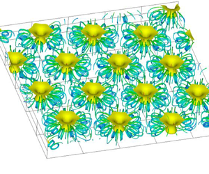
Next, we discuss the transport phenomena of cells and oxygen in three-dimensional bioconvection at high Rayleigh number. Figure 5 shows the flow field and concentration field for  $Ra=5000$. In the cell concentration contours shown in figure 5(a), it is observed that the cells accumulating near the free surface fall towards the bottom at
  $x/h=5.7$ and diffuse to the surroundings. This area of high cell concentration is a plume, and bioconvection occurs around this plume. In addition, as can be seen from figure 5(d), multiple plumes are formed in the suspension. The formation of plumes has also been confirmed in earlier experimental studies (Bees & Hill Reference Bees and Hill1997; Jánosi, Kessler & Horváth Reference Jánosi, Kessler and Horváth1998; Czirók et al. Reference Czirók, Jánosi and Kessler2000) and numerical analyses (Ghorai & Hill Reference Ghorai and Hill2000; Chertock et al. Reference Chertock, Fellner, Kurganov, Lorz and Markowich2012; Karimi & Paul Reference Karimi and Paul2013). Chertock et al. (Reference Chertock, Fellner, Kurganov, Lorz and Markowich2012) and Ghorai & Hill (Reference Ghorai and Hill2000) conducted two-dimensional numerical analysis, and Karimi & Paul (Reference Karimi and Paul2013) performed three-dimensional numerical analysis. However, these works did not show the three-dimensional behaviour of bioconvection. As shown in figure 5(d), this study was able to capture multiple three-dimensional plumes. In figure 5(b), more oxygen is transported towards the bottom wall in the region with the plume. This is because the bioconvection draws the fluid around the plume downwards, increasing the oxygen transport due to the convection. It can be seen from figure 5(d) that the number of plumes generated in the suspension increased compared to the flow field at
  $Ra=500$, and that the distance between the plumes decreased. It is found from the velocity vectors that the downward flow towards the bottom wall occurs at the centre of a plume. Inversely, it is observed that the upward flow towards the free surface occurs between the plumes, and that the velocity is slower than that of the downward flow. Near the water surface, surrounding fluid concentrates toward the plume centre, so cells gather in the plume. As a result, a descending flow of high-concentration suspension occurs toward the bottom wall. Near the lower wall, the flow diffuses from the plume to the surroundings, so the ascending flow velocity between the plumes is slower than the downward flow velocity. This phenomenon can also be explained by the mathematical model used. It can be seen that if more cells are transported downwards by the plume, then the downward flow velocity will increase because the downward volume force in the fundamental equation will increase. The descending and ascending flow velocities are faster than those at
  $Ra=500$, and the bioconvection is stronger. It is observed from the streamlines that three-dimensional vortex rings arise around the plumes because the cells falling towards the bottom wall draw in the surrounding fluid.

Figure 5. (a) Bacterial and (b) oxygen concentration contours, (c) velocity vectors, at  $z/h=4.0$, and (d) isosurface of bacterial concentration, and streamlines for
  $Ra=5000$: isosurface value is 1.2.
For  $Ra=5000$, using the random numbers used in (3.1), we added 1 % and 10 % disturbances to the obtained steady-state cell concentration, and continued the calculation. The converged results were the same as those before the disturbance, and the pattern of bioconvection did not change. The pattern did not change even with different initial disturbances. The suspension is stable with respect to the disturbances. Next, we perturbed the parameters related to the properties of bacteria and oxygen, and investigated the effects of parameter changes on the pattern. In the present study, parameters
  $\beta$,
  $\gamma$ and
  $\delta$ were increased by 1 %. We calculated three cases: (
 $\beta =1.01$,
  $\gamma =\delta =2$), (
 $\beta =1$,
  $\gamma =2.02$,
  $\delta =2$) and (
 $\beta =1$,
  $\gamma =2$,
  $\delta =2.02$). As a result, the pattern did not change, and there was no significant change in the flow or concentration field. From these results, we found that steady bioconvection is strongly stable with respect to disturbances.
Metcalfe & Pedley (Reference Metcalfe and Pedley1998) investigated the patterns formed at the onset of bioconvection, and clarified that the pattern is determined by the physical properties of bacteria and oxygen, such as the strength of oxygen consumption, the strength of directional swimming, and the diffusion coefficient of oxygen. Existing numerical simulations (Chertock et al. Reference Chertock, Fellner, Kurganov, Lorz and Markowich2012; Lee & Kim Reference Lee and Kim2015) have shown that changing the physical properties of bacteria and oxygen causes various bioconvection patterns. In the present study, we investigated the pattern of bioconvection by fixing these parameters and changing the Rayleigh number and initial disturbance. As will be shown later, at a high Rayleigh number, various patterns occurred when only the initial disturbance was changed. Therefore, since the stable steady-state bioconvection pattern varies depending on the initial disturbance, we can speculate that boundary conditions determine the pattern. Since the present study uses periodic boundary conditions, the initial disturbance can freely change not only the cell concentration at the boundary, but also the velocity and oxygen at the boundary, so that the bioconvection pattern can also vary. In § 4.8, we present calculation results for changing the chamber boundary to the side wall to investigate the effect of boundary conditions on bioconvection patterns.
4.3. Effect of physical properties of bacteria and oxygen
Theoretically, the cell and oxygen concentration distributions in a stationary fluid in a shallow chamber do not depend on the parameter  $\delta$ (oxygen versus cell diffusion), but rather change only with the parameters
  $\beta$ (oxygen consumption versus oxygen diffusion) and
  $\gamma$ (directed versus random cell swimming) (Hillesdon & Pedley Reference Hillesdon and Pedley1996). In shallow chambers, there is enough oxygen for bacteria to be active. Hillesdon & Pedley (Reference Hillesdon and Pedley1996) called
  $\beta$ (or
  $\beta \gamma$) depth parameters and investigated the effects of these parameters,
  $\delta$ and
  $\beta \gamma$, on the instability of suspension. As a result, when
  $\beta \gamma$ was changed with fixed
  $\delta$, the minimum value of the critical Rayleigh number that made the suspension unstable appeared. In addition, when
  $\delta$ increased with fixed
  $\beta \gamma$, the critical Rayleigh number increased. In the present study, to clarify the effect of parameters on bioconvection, we investigate the bioconvection when the parameters
  $\delta$ and
  $\beta \gamma$ are changed under the conditions
  $Ra=500$ and 5000 in which bioconvection occurs.
First, we consider the condition that the diffusion coefficient of oxygen to bacteria is large (the diffusion coefficient of bacteria is small). For  $Ra=500$, which is close to the critical Rayleigh number,
  $\delta$ was increased with fixed
  $\beta \gamma$. Figure 6 shows the oxygen concentration distribution and directional swimming velocity magnitude
  $V=|H(c)\,\gamma \,\boldsymbol {\nabla } c|$ at
  $\beta =1$,
  $\gamma =2$ and
  $\delta =5, 10, 20$. The theoretical value and the result of
  $\delta =2$ are also shown for comparison. The cross-section is at the centre of the plume, and its position is
  $(x/h, z/h)=(6.6, 8.0)$ for
  $\delta =5.0$,
  $(x/h, z/h)=(9.2, 2.6)$ for
  $\delta =10$, and
  $(x/h, z/h)=(1.7, 7.6)$ for
  $\delta =20$. As
  $\delta$ increases, more oxygen is transported to the bottom, and the gradient of oxygen concentration in the
  $y$-direction increases, thus increasing the upward directional swimming velocity. This result leads to a decrease in cell transport due to convection (downward flow and upward directional swimming) inside plumes, which also decreases nonlinear effects. Therefore, the bioconvection decays. To compare the strength of convection, we calculated the average kinetic energy in the computational domain. The average kinetic energies are
  $K_{av}=1.56$, 1.03, 0.90, and 0.84 for
  $\delta =2$, 5, 10 and 20, respectively, and the kinetic energy attenuates as
  $\delta$ increases. Although
  $\delta$ was increased to
  $\delta =20$, the bioconvection did not disappear. The directional swimming velocity in figure 6 is the result of the plume centre. We calculated the average value
  $V_{av}$ of the magnitude of the directional swimming velocity in the computational domain. For
  $\delta =2$, 5, 10 and 20,
  $V_{av}=0.542$, 0.540, 0.538 and 0.537, respectively. As
  $\delta$ increases,
  $V_{av}$ decreases slightly but remains almost unchanged. This result suggests that the increase in directional swimming velocity in the plume significantly affects the attenuation of bioconvection. The numbers of plumes are 8, 5, 4 and 4 for
  $\delta =2$, 5, 10 and 20, respectively, and the number of plumes decreases as
  $\delta$ increases. From the above investigation, we find that increasing
  $\delta$ attenuates bioconvection.

Figure 6. Distributions of (a) oxygen concentration and (b) directional velocity.
Next, we investigate the effect of bacteria–oxygen interaction on bioconvection at a high Rayleigh number. Figures 7 and 8 show the results for  $\beta =0.1$ (
 $\beta \gamma =0.2$) and
  $\beta =2$ (
 $\beta \gamma =4$) at
  $\delta =2$, respectively. In figure 8(d), the plume is observed from below. When
  $\beta =0.1$, oxygen consumption by bacteria is suppressed. Chemotactic bacteria respond to oxygen gradients and consume oxygen. When oxygen consumption decreases, bacterial activity declines because the bacteria themselves do not generate oxygen gradients. Therefore, the bioconvection at
  $\beta =0.1$ is weaker than the result at
  $\beta =1$ in figure 5. For
  $\beta =2$, the convective velocity is higher than the result for
  $\beta =1$, and more bacteria and oxygen are transported to the vicinity of the bottom surface. An increase in
  $\beta$ means that the oxygen consumption by bacteria strengthens. As can be seen from the oxygen concentration distribution in figure 8, the oxygen consumption by bacteria increases the oxygen concentration gradient and strengthens directional swimming. At
  $Ra=5000$, the upward and downward flows are strong, and if the directional swimming velocity increases further, then the convection is strengthened on average in the suspension. To compare the strength of directional swimming, we calculated the average magnitude
  $V_{av}$ of the directional swimming velocity in the computational domain. For
  $\beta =0.1$, 1 and 2,
  $V_{av}=6.4\times 10^{-3}$,
  $4.8\times 10^{-1}$ and 1.7, respectively, and the directional swimming velocity at
  $\beta =2$ is 273 times faster than that at
  $\beta =0.1$. This result shows that the bioconvection at
  $\beta =0.1$ is considerably attenuated even at the high Rayleigh number. The numbers of plumes are 8, 15 and 23 for
  $\beta =0.1$, 1 and 2, respectively, and the number of plumes increases as
  $\beta$ increases. From the above results, we found that the rate of oxygen consumption by bacteria significantly affects the strength of bioconvection.

Figure 7. (a) Bacterial and (b) oxygen concentration contours, (c) velocity vectors at  $z/h=0.8$, and (d) isosurface of bacterial concentration, and streamlines for
  $\beta =0.1$ and
  $Ra=5000$: isosurface value is 1.06.

Figure 8. (a) Bacterial and (b) oxygen concentration contours, (c) velocity vectors at  $z/h=1.4$, and (d) isosurface of bacterial concentration, and streamlines for
  $\beta =2$ and
  $Ra=5000$: isosurface value is 1.25.
We investigate the enhancement of convection when directional swimming is increased without changing the rate of oxygen consumption by bacteria. Figure 9 shows the results for  $\delta =2$ and
  $\gamma =10$ (
 $\beta \gamma =10$). An increase in
  $\gamma$ means an increase in the directional swimming velocity of bacteria. The bioconvection is stronger than the results for
  $\gamma =2$ (
 $\beta \gamma =2$) in figure 5 and
  $\beta =2$ (
 $\beta \gamma =4$) in figure 8. The same effect as enhancement of convection with increasing
  $\beta$ appears. The plumes arrange randomly, and the number of plumes is 25. As the number of plumes increases, it is considered that the interference between plumes increases. The average magnitude of directional swimming velocity is
  $V_{av}=9.8$, and the transport by directional swimming increases more than the results for
  $\beta =0.1$ (
 $\beta \gamma =0.2$),
  $\beta =1$ (
 $\beta \gamma =2$) and
  $\beta =2$ (
 $\beta \gamma =4$).

Figure 9. (a) Bacterial and (b) oxygen concentration contours, (c) velocity vectors at  $z/h=4.0$, and (d) isosurface of bacterial concentration, and streamlines for
  $\gamma =10$ and
  $Ra=5000$: isosurface value is 1.46.
We confirmed that the bioconvection and its pattern observed in figures 7–9 were different from the result in figure 5. Although the Rayleigh number and initial disturbance are the same, the different bioconvections and patterns occur even if the parameters related to the physical properties of bacteria and oxygen are changed. This trend is the same as the result of the existing numerical simulations (Chertock et al. Reference Chertock, Fellner, Kurganov, Lorz and Markowich2012; Lee & Kim Reference Lee and Kim2015).
We clarify the effects of changes in the physical properties of bacteria and oxygen on the enhancement of bioconvection and the amount of transport. For  $\beta =0.1$ (
 $\beta \gamma =0.2$),
  $\beta =1$ (
 $\beta \gamma =2$),
  $\beta =2$ (
 $\beta \gamma =4$),
  $\gamma =5$ (
 $\beta \gamma =5$) and
  $\gamma =10$ (
 $\beta \gamma =10$), figure 10 shows the average kinetic energy
  $K_{av}$ and the integral values,
  $N$ and
  $C$, of the amounts of cell and oxygen, respectively. The depth parameter
  $\beta \gamma$ is a parameter of the chamber depth and, at the same time, represents the parameters of the oxygen consumption rate by bacteria and the magnitude of the directional swimming velocity. In a convection-free concentration field in a shallow chamber, theoretically, the cell concentration depends only on
  $\beta \gamma$, while the oxygen concentration varies with
  $\beta \gamma$ and
  $\gamma$ (Hillesdon & Pedley Reference Hillesdon and Pedley1996). The average kinetic energy increases with the increase of
  $\beta \gamma$, indicating that bioconvection strengthens. The oxygen consumption rate by bacteria or directional swimming velocity increases nonlinearity and enhances convection. At this time, cell transport is improved, so many bacteria move to the vicinity of the lower wall. The cell amount decreases slightly near the water surface. Since an increase in
  $\beta \gamma$ increases the consumption of oxygen, the oxygen amount near the water surface and lower wall decreases. For
  $\beta \gamma =5$ (
 $\beta =1, \gamma =5$) and
  $\beta \gamma =10$ (
 $\beta =1, \gamma =10$), the consumption rate of oxygen by bacteria is low, so the oxygen amount does not decrease monotonically. Unlike the cell concentration, the oxygen concentration does not depend only on
  $\beta \gamma$, and this trend is the same as the theory (Hillesdon & Pedley Reference Hillesdon and Pedley1996).

Figure 10. (a) Average kinetic energy. (b) Integral values of bacteria and oxygen.
4.4. Bioconvection pattern and wavelength of the pattern
In this subsection, we discuss the influence of the initial disturbance on the bioconvection pattern and the effect of the Rayleigh number  $Ra$ on the wavelength of the pattern. Figure 11 shows cell concentration contours on the free surface for
  $Ra=500$, 1000, 3000 and 5000. The numbers (e.g. ‘No. 2’) correspond to the pattern names described in table 1, with a higher contour level indicating a higher cell concentration. The plume is formed in the dark-coloured region. In figures 11(b)–11( f), the high concentration regions appear to connect adjacent plumes. Since such a pattern looks like spokes, it was called a spoke pattern in an earlier study (Mazzoni et al. Reference Mazzoni, Giavazzi, Cerbino, Giglio and Vailati2008). Mazzoni et al. (Reference Mazzoni, Giavazzi, Cerbino, Giglio and Vailati2008) reported that the spoke patterns have been observed in previous studies on bioconvection (Platt Reference Platt1961; Jánosi et al. Reference Jánosi, Kessler and Horváth1998; Czirók et al. Reference Czirók, Jánosi and Kessler2000). The present study was able to confirm the spoke pattern as shown in previous studies.

Figure 11. Bacterial concentration contours in the  $x$–
$x$– $z$ plane at
  $y/h=1.0$: (a) No. 2 (
 $Ra=500$); (b) No. 11 (
 $Ra=1000$); (c) No. 13 (
 $Ra=3000$); (d) No. 16 (
 $Ra=5000$); (e) No. 17 (
 $Ra=5000$); ( f) No. 21 (
 $Ra=5000$).
Table 1. Rayleigh number  $Ra$, arrangement of plumes, shape of plumes and pattern wavelength
  $\lambda /h$.

Next, the arrangement of the plumes in the bioconvection patterns is compared. As shown in figures 11(a) and 11(d), the plumes appear in a ‘staggered arrangement’. The plumes in figures 11(b), 11(c) and 11(e) appear to have a ‘lattice arrangement’. In both the staggered and lattice arrangements, the plumes are arranged regularly. This regular plume arrangement has also been observed in a previous experiment on bioconvection (Bees & Hill Reference Bees and Hill1997) and a numerical analysis (Karimi & Paul Reference Karimi and Paul2013). In contrast, since the plumes appear irregularly in figure 11( f), this pattern is defined as a ‘random arrangement’.
We also compare the plume shapes of each bioconvection pattern. This study defines the shapes of the plumes by the number of spokes extending from one plume to the adjacent plumes in the spoke pattern. When the number of spokes extending from one plume is 4, 5 or 6, the plume shape is called a tetragon, pentagon or hexagon, respectively. Since no spoke pattern was observed for  $Ra=500$, the plume shape is called a circle. Focusing on the relation between the arrangement and shape of the plumes, the staggered arrangement shown forms a circular or hexagonal plume, while the lattice arrangement gives rise to a tetragonal plume. As can be observed in figure 11( f), tetragonal, pentagonal and hexagonal plumes exist in an erratic mixture in a random arrangement. Such plume shapes have been confirmed in a previous experiment and numerical studies on bioconvection. The experimental result by Bees & Hill (Reference Bees and Hill1997) indicated that tetragonal or hexagonal plumes regularly form arrays in a long-term pattern. This result corresponds to the tetragonal and hexagonal plumes observed in this study. The experiment of Czirók et al. (Reference Czirók, Jánosi and Kessler2000) showed that hexagonal plumes occur at the final pattern mode of bioconvection. A numerical analysis by Karimi & Paul (Reference Karimi and Paul2013) confirmed the formation of a star-shaped plume. As can be seen by observing this plume in detail, a region of high cell concentration extends from one plume to an adjacent plume in five directions. This star-shaped plume is similar to the pentagonal plume defined in this study.
Table 1 shows the plume arrangement, plume shape and wavelength  $\lambda /h$ of the bioconvection pattern for each Rayleigh number. Here, the wavelength of the pattern was calculated using a two-dimensional fast Fourier transform of the cell concentration on the free surface as in previous studies (Bees & Hill Reference Bees and Hill1997; Czirók et al. Reference Czirók, Jánosi and Kessler2000; Williams & Bees Reference Williams and Bees2011; Kage et al. Reference Kage, Hosoya, Baba and Mogami2013). First, we investigate the influence of the given initial disturbance in the cell concentration on the bioconvection patterns. This study used the initial cell concentration with ten different disturbances for
  $Ra=500$ and 5000. At
  $Ra=500$, the circular plumes showed a staggered arrangement for many of the calculation conditions, and no significant changes in the bioconvection pattern due to the initial disturbance were observed. In contrast, for
  $Ra=5000$, various bioconvection patterns, including the staggered, lattice and random arrangements, occur due to the initial disturbances. This result indicates that even for the same Rayleigh number, bioconvection patterns with different plume arrangements, shapes and numbers can arise due to the effects of different kinds of initial disturbances, and that the wavelengths of the bioconvection patterns are different. In a previous experiment (Bees & Hill Reference Bees and Hill1997), it was reported that it is difficult to achieve a homogeneous cell concentration as the ideal initial state of the suspension because fluid motion after mixing the suspension remains. Bees & Hill (Reference Bees and Hill1997) found that the wavelengths of the bioconvection patterns also varied, accompanying the pattern change, even though the same cell concentration and suspension depth were set. In this study, initial disturbances are added to the initial conditions of the cell concentration to simulate the initial state in the previous experiment (Bees & Hill Reference Bees and Hill1997). From this result, it can be concluded that the present study confirms the phenomenon observed in the previous study. As mentioned above, it is found that more significant changes in the bioconvection pattern due to the initial disturbance appear at high Rayleigh number because the increase in the Rayleigh number enhances the nonlinearity. Finally, comparing the wavelengths of the patterns in table 1, it is confirmed that the wavelengths of the bioconvection patterns are changed depending on the plume arrangement. In addition, the wavelength of the pattern becomes shorter as the Rayleigh number increases.
4.5. Wavelength comparison with previous results
Next, we compare this numerical result with previous results for the wavelengths of bioconvection patterns. Bees & Hill (Reference Bees and Hill1997) conducted experiments on bioconvection formed by single-celled alga Chlamydomonas nivalis and investigated the wavelengths of the bioconvection patterns at the onset of bioconvection and in a long-term pattern. They found that the wavelength decreases with increasing cell concentration and that the cell concentration has a significant effect on the wavelength of the pattern. Czirók et al. (Reference Czirók, Jánosi and Kessler2000) investigated experimentally the bioconvection formed by Bacillus subtilis and measured the wavelength of the bioconvection pattern at the onset of bioconvection. They clarified that the wavelength decreases with increasing cell concentration measured by optical density measurements. To compare our numerical results with earlier experimental results using the Rayleigh number, we calculated the Rayleigh number of the experimental data. The volume of a cell  $V$, density ratio of a cell to water
  $(\rho _n-\rho )/\rho$, water kinematic viscosity
  $\nu$, and cell diffusivity
  $D_{n0}$ were not described in the Bees & Hill paper, so we used values from Ghorai & Hill (Reference Ghorai and Hill2002). Likewise,
  $V$,
$V$,  $(\rho _n-\rho )/\rho$,
  $\nu$ and
  $D_{n0}$ were not mentioned in Czirók et al. (Reference Czirók, Jánosi and Kessler2000), so we took
  $\nu$ from Hillesdon & Pedley (Reference Hillesdon and Pedley1996), and other values from Jánosi et al. (Reference Jánosi, Kessler and Horváth1998). The gravity acceleration
  $g$ was not reported in these papers (Hillesdon & Pedley Reference Hillesdon and Pedley1996; Bees & Hill Reference Bees and Hill1997; Jánosi et al. Reference Jánosi, Kessler and Horváth1998; Czirók et al. Reference Czirók, Jánosi and Kessler2000; Ghorai & Hill Reference Ghorai and Hill2002), thus we took
  $g$ from Pedley, Hill & Kessler (Reference Pedley, Hill and Kessler1988). The numerator of the Rayleigh number equation (2.10a–e) defined in this paper includes the initial cell concentration
  $n_0$. Thus it can be considered that increasing the Rayleigh number increases the initial cell concentration.
Figure 12 shows a comparison between our numerical values and experimental values (Bees & Hill Reference Bees and Hill1997; Czirók et al. Reference Czirók, Jánosi and Kessler2000) for the bioconvection pattern. The trend of the wavelength of the pattern to decrease with increasing Rayleigh number is qualitatively consistent with the experimental results. However, there is a quantitative difference between the wavelengths in this calculation and the experiments.

Figure 12. Comparison of pattern wavelength with previous results (Bees & Hill Reference Bees and Hill1997; Metcalfe & Pedley Reference Metcalfe and Pedley1998; Czirók et al. Reference Czirók, Jánosi and Kessler2000; Chertock et al. Reference Chertock, Fellner, Kurganov, Lorz and Markowich2012; Lee & Kim Reference Lee and Kim2015). (a) Comparison with experiment. (b) Comparison with calculation.
Metcalfe & Pedley (Reference Metcalfe and Pedley1998) used weakly nonlinear analysis to determine the critical wavenumber and critical Rayleigh number at which a suspension becomes unstable. We obtained the wavelength at the critical Rayleigh number for two conditions ( $\gamma \beta =1$,
  $\delta =1$,
  $Sc=7700$) and (
 $\gamma \beta =50$,
  $\delta =1$,
  $Sc=7700$) in the existing research. In addition, using the previous calculations (Chertock et al. Reference Chertock, Fellner, Kurganov, Lorz and Markowich2012; Lee & Kim Reference Lee and Kim2015), we calculate the wavelength of the bioconvection pattern generated when an initial disturbance is given by random numbers. The parameters in the calculation of Chertock et al. (Reference Chertock, Fellner, Kurganov, Lorz and Markowich2012) are
  $\beta =4$,
  $\gamma =10$,
  $\delta =5$ and
  $Sc=500$, and the parameters in the calculation of Lee & Kim (Reference Lee and Kim2015) are
  $\beta =2$,
  $\gamma =10$,
  $\delta =5$ and
  $Sc=500$. We calculated the wavelength from the number of plumes and the length of the calculation area. Figure 12(b) compares the wavelength derived from the previous results with the present results. In all analyses using chemotactic bacteria, the parameters used are different, but the previous results are in the range
  $\lambda /h=2.0\unicode{x2013}4.0$. These values are overestimated as compared to the experimental values for all Rayleigh numbers. Thus further investigations into this difference are required.
Earlier studies (Bees & Hill Reference Bees and Hill1997; Ghorai & Hill Reference Ghorai and Hill2002; Williams & Bees Reference Williams and Bees2011) reported similarities between bioconvection and thermal convection. Therefore, the patterns observed in previous experiments for thermal convection (Koschmieder & Switzer Reference Koschmieder and Switzer1992) and in numerical analysis (Tomita & Abe Reference Tomita and Abe2000), and the wavelengths of the patterns, are compared with the present values. Koschmieder & Switzer (Reference Koschmieder and Switzer1992) showed that the number of convection cells increased as the temperature difference applied to the fluid increased. In that paper, the Rayleigh number is defined, and an increase in temperature difference corresponds to an increase in the Rayleigh number. An increase in the number of convection cells means a decrease in the spacing between convection cells, that is, the wavelength of the pattern. Tomita & Abe (Reference Tomita and Abe2000) investigated Bénard–Marangoni convection and found that the wavelength of the pattern decreases as the parameter that combines the Rayleigh and Marangoni numbers increases. Increasing this parameter means increasing the Rayleigh number. Therefore, it can be said that the trend of the wavelength of the bioconvection pattern to decrease with increasing Rayleigh number is qualitatively consistent with the result of thermal convection. Furthermore, when comparing the patterns, the hexagonal convection pattern observed in the previous studies (Koschmieder & Switzer Reference Koschmieder and Switzer1992; Tomita & Abe Reference Tomita and Abe2000) is similar to the hexagonal-shaped plume observed in the present study. The wavelength of the hexagonal convection pattern (Tomita & Abe Reference Tomita and Abe2000) is  $2.71 \leqslant \lambda /h \leqslant 2.94$, which is similar to the wavelength of the bioconvection pattern observed in this study.
4.6. Interference between plumes
We discuss the influence of the wavelength variation of the bioconvection pattern on the concentration field. First, figures 13 and 14 show the distribution of cell and oxygen concentrations in the  $y$-direction at the plume centre and between plumes. Here, No. 2 (
 $Ra=500$), No. 11 (
 $Ra=1000$), No. 12 (
 $Ra=2000$), No. 13 (
 $Ra=3000$), No. 14 (
 $Ra=4000$) and No. 16 (
 $Ra=5000$) in table 1 are used for the results. All these results used the same initial disturbance. We consider the positions at the plume centre and between the plumes as being the points where the cell concentrations on the free surface become maximum and minimum, respectively. The positions of the plume centres at
  $Ra=500$, 1000, 2000, 3000, 4000, 5000 are
  $(x/h, z/h) = (4.7, 0.4)$,
  $(5.8, 3.2)$,
  $(8.0, 0.5)$,
  $(1.9, 3.5)$,
  $(1.5, 8.8)$,
  $(2.3, 0.8)$, and the positions between the plumes are
  $(x/h, z/h) = (3.4, 1.6)$,
  $(5.8, 8.2)$,
  $(3.0, 6.2)$,
  $(6.9, 8.5)$,
  $(7.7, 2.6)$,
  $(6.1, 2.6)$.

Figure 13. Bacterial concentration distributions in the  $y$-direction at (a) the centre of the plume, (b) between plumes.

Figure 14. Oxygen concentration distributions in the  $y$-direction at (a) the centre of the plume, (b) between plumes.
In the centre of the plume, as the wavelength of the pattern decreases, the amount of the cell transported by the downward flow increases, so the cell concentration near the water surface decreases. As can be seen from figures 4 and 5, bioconvection strengthens as the wavelength of the pattern decreases, and the plume extending to the lower wall diffuses to the surroundings. This indicates that the cell amount transported from the plume centre to between the plumes increases. Therefore, as the wavelength decreases, the cell concentration near the lower wall decreases at the plume centre, converges to a constant value, and increases between the plumes. The cell concentration near the water surface between the plumes does not change depending on the wavelength, except at  $Ra=500$, and is lower than the concentration at the plume centre. At
  $Ra=500$, the bioconvection is weak, so the trend is different from the results at other Rayleigh numbers.
Next, we consider the oxygen concentration. At the plume centre, the oxygen concentration near the lower wall increases because the oxygen transported by the downward flow increases as the wavelength of the pattern decreases. Between the plumes, the oxygen concentration decreases at  $\lambda /h>2.77$ (
 $Ra<3000$) as the wavelength decreases. This is because as the wavelength decreases, the amount of cells transported between plumes increases, and the amount of oxygen consumed increases. On the other hand, the tendency of
  $\lambda /h \leqslant 2.77$ (
 $Ra \geqslant 3000$) is different from the result of
  $\lambda /h>2.77$ (
 $Ra<3000$), and the oxygen concentration increases as the wavelength decreases. This is because as the wavelength decreases, bioconvection strengthens and the amount of oxygen transported between plumes exceeds the amount of oxygen consumed by bacteria.
This study calculated the mean velocity  $v_{down}$ of the downward flow at the centre of the plume, and the mean velocity
  $v_{up}$ of the upward flow between plumes. Here,
  $v_{down}$ and
  $v_{up}$ are defined by averaging the vertical velocities such that
  $v < 0$ and
  $v > 0$, respectively. Figure 15(a) shows the relationship between the wavelength of the pattern and mean velocities
  $v_{down}$ and
  $v_{up}$. In the figure, the wavelength of the pattern decreases as the Rayleigh number increases, then
  $|v_{down}|$ increases at the centre of the plume. Also, we can observe the same tendency in
  $v_{up}$ between the plumes shown in the figure. This result occurs because the interference between plumes has increased. In other words, as the wavelength of the pattern becomes shorter, the plumes approach each other, and the velocities of the downward flow and the upward flow increase. In addition, we have observed in figure 5 that the velocity of the downward flow is faster than that of the upward flow. The wavelengths of the patterns for
  $Ra=2000$ and
  $3000$ have the same values. However, as can be seen from
  $|v_{down}|$ and
  $v_{up}$, the flow velocities of
  $Ra=3000$ are faster than those of
  $Ra=2000$. This result is because the number of cells transported downwards increases as the Rayleigh number increases, and then the bioconvection is strengthened.

Figure 15. Mean velocities of downward and upward flows: (a) mean velocity, (b) velocity ratio.
Figure 15(b) shows the ratio of the downward velocity to the upward velocity. This ratio is also related to the volume occupied by the plumes and the volume occupied between the plumes. As can be seen in figure 5, the plumes with high cell concentrations are narrower than the areas between the plumes. Figure 15(b) shows that if the net upward and downward transports are balanced on average, then the velocity of the descending flow in the plume will be faster than that of the upward flow, and the area occupied by the plume will become small. When the wavelength is large, the velocity ratio reaches 3, and the area of influence of the downward flow in the plume on the cell transport becomes narrow. As the wavelength decreases, the velocity ratio decreases. This suggests that the ascending flow velocity increases and the area of influence of the ascending flow on the cell transport becomes narrow.
To compare the strength of convection in each pattern, the average kinetic energy within the calculation domain was calculated for  $Ra=5000$. If the kinetic energy is high, then it can be said that the convection is strong on average. The mean value obtained from the average kinetic energy of all patterns was
  $K_{av}=47.2$, and the standard deviation was 0.341. We find that the strength of bioconvection does not depend on the pattern.
We investigate the influence of the shear flow near the wall surface on bacteria. The surface friction coefficient  $C_f$ on the bottom wall is defined as
  $C_f=\tau _w/[\rho (D_{n0}/h)^2/2]$, where
  $\tau _w=\mu (\partial V/\partial y)$, and
  $V$ is a composite component of the velocities in the
  $x$- and
  $z$-directions. Figures 16 and 17 show the contours of the cell concentration at
  $y/h=0.01$ and the surface friction coefficient using the data of No. 11 (
 $Ra=1000$), No. 13 (
 $Ra=3000$) and No. 16 (
 $Ra=5000$) in table 1. The same initial disturbance is applied to all these results. In the region where the plumes exist, the cell concentration becomes high, and it can be seen that a large amount of bacteria exists under the plumes. Comparing the results for each Rayleigh number, we observe that the cell concentration decreases in the centre of a plume and increases between the plumes as the wavelength of the bioconvection pattern decreases. It is found that the surface friction coefficient is large in the region of a plume and that a strong shear flow occurs in this region. Also, the wall friction coefficient increases as the wavelength of the pattern decreases. Therefore, the cells under the plumes are affected by strong shear stress. Van der Pol & Tramper (Reference Van der Pol and Tramper1998) investigated the influence of shear stress on animal cells, and reported that shear stress causes damage to animal cells and cell death. In future research, it will be interesting to investigate the influence of shear stress on bacteria due to bioconvection.

Figure 16. Bacterial concentration contours in the  $x$–
$x$– $z$ plane at
  $y/h=0.01$ for
  $Ra=1000$, 3000, 5000: (a)
  $\lambda /h=3.16$ (
 $Ra=1000$); (b)
  $\lambda /h=2.77$ (
 $Ra=3000$); (c)
  $\lambda /h=2.43$ (
 $Ra=5000$).

Figure 17. Surface friction coefficient contours in the  $x$–
$x$– $z$ plane at the lower wall for
  $Ra=1000$, 3000, 5000: (a)
  $\lambda /h=3.16$ (
 $Ra=1000$); (b)
  $\lambda /h=2.77$ (
 $Ra=3000$); (c)
  $\lambda /h=2.43$ (
 $Ra=5000$).
4.7. Transport characteristics
To clarify the transport characteristics of cells and oxygen, we investigated the variations of each flux distribution. As in previous studies (Yanaoka et al. Reference Yanaoka, Inamura and Suzuki2007, Reference Yanaoka, Inamura and Suzuki2008), the flux of cells and oxygen is defined as
 $$\begin{gather} J_{n}^{{total}} = J_{n}^{{conv}} + J_{n}^{{diff}} + J_{n}^{{swim}}, \end{gather}$$
 $$\begin{gather}J_{c}^{{total}} = J_{c}^{{conv}} + J_{c}^{{diff}}, \end{gather}$$
where  $J_n^{total}$ is the total flux of cells,
  $J_c^{total}$ is the total flux of oxygen,
  $J_n^{conv}$ is the convective flux of cells,
  $J_c^{conv}$ is the convective flux of oxygen,
  $J_n^{diff}$ is the diffusive flux of cells,
  $J_c^{diff}$ is the diffusive flux of oxygen, and
  $J_n^{swim}$ is the swimming flux of cells. These fluxes are given as
 $$\begin{gather} J_{n}^{{conv}} = \boldsymbol{u} n, \quad J_{n}^{{diff}} ={-} H(c)\,\boldsymbol{\nabla} n, \quad J_{n}^{{swim}} = H(c)\,\gamma n\,\boldsymbol{\nabla} c, \end{gather}$$
 $$\begin{gather}J_{c}^{{conv}} = \boldsymbol{u} c, \quad J_{c}^{{diff}} ={-} \delta\,\boldsymbol{\nabla} c . \end{gather}$$
 For  $Ra=1000$, 3000 and 5000, figures 18 and 19 show the cell and oxygen flux distributions in the
  $y$-direction at the centre of a plume and between the plumes, respectively. The results shown are for a lattice arrangement (figures 11b,c,e) in which plumes are arrayed regularly. For
  $Ra=1000$, 3000 and 5000, the positions of the plume centres are
  $(x/h, z/h)=(5.8, 3.2)$,
  $(1.9, 3.5)$ and
  $(6.2, 6.0)$, and the positions between the plumes are
  $(x/h, z/h)=(5.8, 8.2)$,
  $(6.9, 8.5)$ and
  $(1.2, 6.0)$. At the centre of a plume, the cell and oxygen transport due to the convection are dominant throughout the region. In the velocity vectors shown in figure 5, the convective velocity increased near
  $y/h=0.6$, where the flows around the plume joined together. Thus the transport by the convection becomes active there. These trends are similar between the plumes, but because the convective velocity between the plumes is slower, the convective transport between the plumes becomes smaller than that at the centre of a plume. The flux ratios are also shown in figures 18 and 19. The previous study (Chertock et al. Reference Chertock, Fellner, Kurganov, Lorz and Markowich2012) also discussed transport characteristics using the flux ratio. Near the lower wall and the water surface in the centre of the plume, the cell transport by random swimming (diffusion) and directional swimming, and the oxygen transport by diffusion, increase compared to the transport by convection. At small wavelengths, the transport by directional swimming is slightly larger than the transport by random swimming. In contrast, the cell transport by diffusion and swimming is large near the free surface between the plumes, and the cells are actively moving. Here, the cell transport due to the directional and random swimming is almost in balance. Since the oxygen is supplied from the free surface of the suspension by diffusion, the oxygen transport increases towards the free surface. The flux ratios indicate that the transport by swimming and diffusion between the plumes is relatively larger than the transport by convection, as compared to the centre of the plume, because the convective transport by the upward flow is smaller than that by the downward flow.

Figure 18. Flux distributions of bacteria and oxygen in the  $y$-direction at the centre of a plume: (a) bacteria; (b) bacteria (flux ratio); (c) oxygen; (d) oxygen (flux ratio).

Figure 19. Flux distributions of bacteria and oxygen in the  $y$-direction between plumes: (a) bacteria; (b) bacteria (flux ratio); (c) oxygen; (d) oxygen (flux ratio).
Next, we compare the transport characteristics of cells and oxygen for each wavelength of the bioconvection pattern. The total fluxes of cells and oxygen increase with decreasing wavelength at plume centres and between the plumes. The reason is as follows. The wavelength decrease enhances interference between plumes, increasing the downward and upward flow velocities at the plume centre and between the plumes. Therefore, the transport of cells and oxygen by convection increases. As can be seen from the flux ratios, the cell transport due to diffusion and swimming is low regardless of wavelength, except near the bottom wall and the water surface. Near the water surface between plumes, the flux ratios vary significantly with the wavelength. As the wavelength decreases, the cell transport by diffusion and swimming, and the oxygen transport by diffusion, decrease compared to the convective transport.
To clarify the influence of the wavelength of the pattern on the transport characteristics over the entire suspension, the integral values of the total flux of cells and oxygen,  $J_n^{int}$ and
  $J_c^{int}$, were evaluated. These values are obtained by integrating
  $|J_n^{total}|$ and
  $|J_c^{total}|$ over the entire suspension. We consider the transport characteristics of cells and oxygen for the downward and upward flows. Figure 20 shows the relationship between
  $J_n^{int}$ and
  $J_c^{int}$ of the total flux of cells and oxygen and the wavelength
  $\lambda /h$ of the pattern. As the Rayleigh number increases, the wavelength decreases and interference between the plumes increases, which improves the transport characteristics of the cells and oxygen due to the downward flow. These trends are similar in the upward flow region. From the above, it can be said that because the transport characteristics due to the downward and upward flows improve with decreasing wavelength, the transport characteristics over the entire suspension also improve.

Figure 20. Integral values of total flux of bacteria and oxygen in the  $y$-direction for (a) downward flow, and (b) upward flow.
To investigate the effects of pattern wavelength changes on the transport of bacteria and oxygen, we calculate the integral values,  $N$ and
  $C$, of the amounts of cells and oxygen, respectively, near the bottom wall (
 $0 \leqslant y/h \leqslant 0.2$), in the middle (
 $0.4 \leqslant y/h \leqslant 0.6$), and near the water surface (
 $0.8 \leqslant y/h \leqslant 1.0$). The results of No. 2 (
 $Ra=500$), No. 11 (
 $Ra=1000$), No. 12 (
 $Ra=2000$), No. 13 (
 $Ra=3000$), No. 14 (
 $Ra=4000$) and No. 16 (
 $Ra=5000$) in table 1 are shown in figure 21. These are the results when the same initial disturbance is given. As the wavelength decreases, the cell amount decreases near the water surface and increases near the bottom wall. This is because the transport characteristics improve as the wavelength decreases, and the cell amount that settles downwards increases. At
  $\lambda /h=3.54$, the difference between the cell amounts near the bottom wall and near the water surface is large, but the difference decreases as the wavelength decreases. The cell amount near the middle increases slightly as the wavelength decreases, but at
  $\lambda /h<3.16$, the cell amount becomes approximately constant. The oxygen amount increases near the bottom wall and in the middle area because the oxygen transport characteristics improve as the wavelength decreases. The oxygen amount near the water surface is approximately constant. Since the bacteria that gather downwards consume oxygen, the oxygen amount decreases towards the depth at each wavelength. It was found from the above results that the amounts of cells and oxygen near the bottom wall increase because the transport characteristics improve as the pattern wavelength decreases.

Figure 21. Integral values of (a) bacterial and (b) oxygen concentrations.
4.8. Influences of computational region and boundary condition
To confirm that the above results do not depend on the calculation region, we compare the results for the computational regions of  $L=10h$ and
  $20h$ for
  $Ra=5000$. The same initial disturbance for
  $L=10h$ in figure 5 was set for
  $L=20h$. Figure 22 shows the flow field and concentration field at
  $L=20h$. As in figure 5, it can be seen that bioconvection with multiple plumes occurs. In the bioconvection pattern in figure 22(d), a lattice arrangement in the region of
  $x/h \geqslant 10$, a staggered arrangement in
  $5 \leqslant x/h \leqslant 10$,
  $z/h \geqslant 10$, and random arrangements in
  $x/h \leqslant 10$,
  $0 \leqslant z/h \leqslant 10$ appear. It is found from this result that the bioconvection patterns observed at
  $L=10h$ appear simultaneously. The wavelength of the bioconvection pattern for
  $L=20h$ is
  $\lambda /h=2.34$. We calculated the averaged wavelength for
  $L=10h$ to compare the results of
  $L=10h$ and
  $20h$. The wavelength was
  $\lambda /h=2.38$, which was obtained by averaging the wavelengths of all patterns for
  $L=10h$. The difference between the wavelengths for
  $L=10h$ and
  $L=20h$ is approximately 1.71 %, and it can be said that the wavelengths of the bioconvection patterns observed at
  $L=10h$ and
  $20h$ are almost the same. As with
  $L=10h$, it is possible that bioconvection patterns with different wavelengths will occur for different initial disturbances.

Figure 22. (a) Bacterial and (b) oxygen concentration contours, (c) velocity vectors at  $z/h=18.8$, and (d) bacterial concentration contours at
  $y/h=1.0$ for
  $Ra=5000$.
Next, we investigate the transport characteristics of the cells and oxygen over the entire suspension for  $L=20h$. The integral values of the total flux are
  $J_n^{int}=1767.2$ and
  $J_c^{int}=1297.9$. To compare the results of
  $L=10h$ and
  $20h$, we averaged the integrated value of the total flux of each pattern for
  $L=10h$, and the values were
  $J_n^{int}=440.8$ and
  $J_c^{int}=323.8$. To compare these values with the result for
  $L=20h$, which is 4 times the computational region of
  $L=10h$,
  $J_n^{int}$ and
  $J_c^{int}$ for
  $L=10h$ are multiplied by 4, and the differences between the results for
  $L=10h$ and
  $L=20h$ are found to be approximately 0.23 % and 0.21 %, respectively. The results for
  $L=10h$ and
  $20h$ are almost the same. Comparing the calculation results for
  $L=10h$ and
  $L=20h$, the same results were obtained for the wavelength and transport characteristics of the bioconvection pattern, even for different computational regions. Therefore, it can be seen that the results for
  $L=10h$ do not depend on the computational region.
The pattern of Rayleigh–Bénard convection changes depending on the system geometry and boundary conditions (Cross & Hohenberg Reference Cross and Hohenberg1993; Bodenschatz, Pesch & Ahlers Reference Bodenschatz, Pesch and Ahlers2000). Similarly, it is considered that the pattern of bioconvection changes. Metcalfe & Pedley (Reference Metcalfe and Pedley1998) mentioned that the side wall of the Petri dish affects the pattern. Yamamoto et al. (Reference Yamamoto, Okayama, Sato and Takaoki1992) also clarified that the vessel's wall determines the pattern generation. Figure 23 shows the calculation result for changing the chamber boundary to side walls. In this calculation, the calculation conditions are the same as those using periodic boundary conditions, and the given initial disturbance is also the same. Plumes line up along the boundaries. A pattern with more regularity than the result in figure 22 occurs. Bacteria adhere to all side walls, and plumes form near the walls. Therefore, downward flow occurs near all side walls. The same regular pattern as in figure 23 was obtained even with different initial disturbances. Since bacteria gather near the water surface before bioconvection occurs, bacteria adhere to the side wall. Subsequently, the suspension becomes unstable, and plumes form. Since the velocity is slow near the wall due to the no-slip condition, the bacteria adhered to the side wall are less likely to come off, and even if bioconvection develops, the bacteria may remain attached to the side wall. The integrated values of the total flux are  $J_n^{int}=1789.5$ and
  $J_c^{int}=1326.0$, and the differences from the results when using the periodic boundary condition are
  $1.3\unicode{x2013}2.2$ %. Therefore, there is no difference in transport characteristics due to the boundary conditions. Karimi & Paul (Reference Karimi and Paul2013) performed a numerical analysis on gyrotactic bioconvection and reported that the pattern at the final stage does not depend on boundary conditions. This trend differs from our calculation results. Since the present result is a converged solution after sufficient time has passed, it is considered that this regular pattern does not collapse. Karimi & Paul (Reference Karimi and Paul2013) reported that the final pattern did not reach a steady state, so this discrepancy with the existing result may be due to the difference between steady state and transient state, but requires further investigation.

Figure 23. (a) Bacterial and (b) oxygen concentration contours, (c) velocity vectors at  $z/h=8.9$, and (d) bacterial concentration contours at
  $y/h=1.0$ for
  $Ra=5000$ in chamber with side walls.
When using the periodic boundary condition, changing the initial disturbance can change not only the cell concentration on the boundary, but also the velocity and oxygen, so that the bioconvection pattern can also vary. If the side wall is set, then bacteria will adhere to the wall surface. Therefore, it is considered that the pattern is difficult to change freely. Since we impose a condition of zero cell flux at the side wall, bacterial adhesion is a natural consequence. However, it is still necessary to investigate the cause of bacteria remaining attached to the side wall. In bioconvection, in which plumes interact with each other, the phenomenon of adhesion of bacteria to walls has not been investigated in detail. Therefore, such investigations will be the subject of future research.
5. Conclusions
We conducted a three-dimensional numerical simulation on bioconvection generated by oxygen-reactive chemotactic bacteria. The bioconvection patterns, interference between plumes, wavelength of the bioconvection pattern, and transport characteristics of cells and oxygen were investigated when multiple plumes occurred in the suspension. The findings obtained are summarized as follows.
(i) When the Rayleigh number reaches the critical value, multiple three-dimensional plumes arise in the suspension. Three-dimensional bioconvection occurs around the plumes, and vortex rings form around the plumes. Even if bioconvection at a high Rayleigh number is disturbed, the bioconvection is strongly stable with respect to disturbances, and the pattern does not change due to disturbances.
(ii) The ratio of the diffusion coefficient of oxygen to bacteria greatly affects the strength of bioconvection, and when the diffusion coefficient of oxygen is relatively large, bioconvection becomes weak. The rate of oxygen consumption by bacteria significantly affects the strength of bioconvection, and the stronger the oxygen consumption by bacteria, the stronger the bioconvection. This trend to strengthen bioconvection is also the same when the directional swimming velocity of bacteria increases.
(iii) Bioconvection patterns with different plume arrangements and shapes are formed for different Rayleigh numbers or initial disturbances of the cell concentration. Thus the wavelengths of the patterns also vary. Comparing the arrangement and shape of the plumes, a staggered arrangement is observed consisting of circular or hexagonal plumes, a lattice arrangement constituted by tetragonal plumes, and a random arrangement consisting of plumes with various shapes.
(iv) As the Rayleigh number increases, interference between the plumes is strengthened by the decrease in wavelength of the pattern. Thus the velocities of both the upward and downward flows increase. The velocity of the downward flow is faster than that of the upward flow.
(v) Many cells are located under plumes, and a strong shear flow occurs in these regions. As the wavelength of the pattern decreases, the shear stress increases. Therefore, many cells are affected by a strong shear stress.
(vi) The convective transport of the entire suspension strengthens as the wavelength of the pattern decreases. Therefore, the transport characteristics of cells and oxygen improve, and then the amounts of cells and oxygen transported near the bottom wall in the suspension increase.
(vii) When the chamber boundary is changed to side walls, bacteria adhere to the wall surface, and plumes are arranged regularly along the side walls. Periodic boundary conditions can cause various patterns of bioconvection, while the side wall may suppress free formations of patterns.
In the present study, we investigated the effect of the chamber side wall on the pattern of bioconvection and found that the side wall changed the pattern. This time, we used a rectangular container with side walls. The chamber geometry may change the pattern of bioconvection and accompanying transport characteristics, so further investigation of bioconvection under different boundary conditions is necessary. In addition, since characteristics such as the oxygen consumption rate of bacteria significantly affect bioconvection, advanced mathematical models are required. More detailed experimental information will be useful for developing mathematical models, and it is thought that the investigation of transport characteristics by numerical analysis will develop. Furthermore, it is necessary to investigate the control of bioconvection for the engineering application of bioconvection. We have investigated the interference between bioconvection and thermal convection by heating suspension and the improvement of transport characteristics, and we plan to report the results in the future.
Acknowledgements
The numerical results in this research were obtained using the supercomputing resources at Cyberscience Center, Tohoku University. We would like to express our gratitude to Associate Professor Y. Suenaga of Iwate University for his support of H.Y.'s laboratory. The authors wish to acknowledge the time and effort of everyone involved in this study.
Funding
This work was supported by Grants-in-Aid for Scientific Research C from Japan Society for the Promotion of Science (grant no. 24560181).
Declaration of interests
The authors report no conflict of interest.
Author contributions
H.Y. conceived and planned the research and developed the numerical method and calculation codes. T.N. performed the simulations. Both authors contributed equally to analysing data and reaching conclusions, and in writing the paper.


