1 Introduction
The generic problem of path oscillations routinely observed with light bodies falling or rising freely in a large expanse of fluid has attracted attention for a very long time, as testified for instance by several of Leonardo da Vinci’s drawings which were concerned with bubbles rising in water. About two centuries later, Newton performed experiments with falling spheres made of various materials, especially wax, glass and lead. In part 2 of his Principia, he discussed experiments carried out by his collaborator Desaguliers with inflated hog bladders released from the top of St. Paul’s cathedral and concluded that their lateral oscillations were responsible for the increase of their falling time compared to that of reference leaden spheres (Eckert Reference Eckert2006). Throughout the 20th century, the subject of the free, gravity- or buoyancy-driven motion of spheres was examined in several series of experiments (see Horowitz & Williamson (Reference Horowitz and Williamson2008) for references). In most cases, the main objective was to compare their drag to that of spheres held fixed in a uniform stream, mostly in the fully turbulent regime. New light was shed on the topic in the 90s, through two nearly simultaneous, albeit independent, streams of work. First, a series of experiments (Karamanev & Nikolov Reference Karamanev and Nikolov1992; Karamanev, Chavarie & Mayer Reference Karamanev, Chavarie and Mayer1996) suggested that, for Reynolds numbers larger than a few hundred, the drag coefficient of light enough rising spheres becomes independent of the Reynolds number and takes a value much larger than that of the corresponding fixed sphere. Second, the first steps of the transition in the wake of fixed spheres started to be studied computationally, first in the framework of linear stability analysis (Natarajan & Acrivos Reference Natarajan and Acrivos1993), then through direct numerical simulation (Johnson & Patel Reference Johnson and Patel1999; Tomboulides & Orszag Reference Tomboulides and Orszag2000). The rapid development of modern optical techniques and the tremendous increase of computer power quickly made it possible to revisit the subject with an improved efficiency, and hopefully a better accuracy.
A major step forward was carried out by Jenny, Dušek & Bouchet (Reference Jenny, Dušek and Bouchet2004), hereinafter referred to as JDB, who examined the transition to chaos of falling and rising spheres as a function of their relative density through a large set of direct simulations. They characterized several intermediate regimes encountered along the route to chaos, revealing complex scenarios in several regions of the parameter space, such as for instance a switch from low- to high-frequency oscillations as the sphere-to-fluid density ratio is increased, or the existence of a large ‘island’ of bi-stability for rising spheres, where fully chaotic three-dimensional paths coexist with planar trajectories exhibiting periodic low-amplitude oscillations. In particular, they evidenced an intermediate Reynolds number range where all rising spheres follow periodic planar low-frequency zigzagging paths with lateral excursions of the order of the sphere diameter. In contrast, no falling sphere was found to display a similar type of path. Detailed experiments were then carried out with spheres of various densities (Veldhuis & Biesheuvel Reference Veldhuis and Biesheuvel2007; Veldhuis, Biesheuvel & Lohse Reference Veldhuis, Biesheuvel and Lohse2009; Ostmann, Chaves & Brüker Reference Ostmann, Chaves and Brüker2017), to determine the styles of path and their structural characteristics (including the wake structure) as a function of the Reynolds number and sphere relative density. The first of these provided a careful comparison with some of JDB’s predictions, while the second attempted to determine conditions under which the non-standard behaviour of the drag coefficient reported by Karamanev & Nikolov (Reference Karamanev and Nikolov1992) and Karamanev et al. (Reference Karamanev, Chavarie and Mayer1996) takes place. A major experimental attack was presented by Horowitz & Williamson (Reference Horowitz and Williamson2010), based on a large combination of sphere-to-fluid density ratios and Reynolds numbers, the latter being varied by changing the sphere size and fluid viscosity. A totally novel behaviour was identified in these experiments. That is, beyond the initial transition that marks the end of the steady vertical rise/fall (which corresponds to the loss of axisymmetry in the wake), spheres with relative densities larger than a critical value close to
 $0.36$
were found to only slightly deviate from vertical whatever the Reynolds number, ascending along a weakly oblique path. The corresponding slope was observed to be uniform below a certain Reynolds number and oscillating intermittently beyond it. In contrast, all spheres with relative densities smaller than
$0.36$
were found to only slightly deviate from vertical whatever the Reynolds number, ascending along a weakly oblique path. The corresponding slope was observed to be uniform below a certain Reynolds number and oscillating intermittently beyond it. In contrast, all spheres with relative densities smaller than
 $0.36$
were found to ‘vibrate’ as soon as the Reynolds number exceeds the critical value corresponding to the onset of shedding in the wake past a fixed sphere. This ‘vibration’ takes the form of virtually planar large-amplitude periodic zigzags and is accompanied by two remarkable characteristics. First, the shedding cycle involves four pair of vortices per zigzag period. This original shedding mode is in stark contrast with the one-sided mode observed with spheres that follow an inclined path, and the two-sided mode involved in the wake of spheres that fall or rise vertically with a large enough Reynolds number. Second, the drag coefficient of all ‘vibrating’ spheres is independent of the Reynolds number and significantly larger than that of the corresponding fixed sphere, although lower than that reported by Karamanev & Nikolov (Reference Karamanev and Nikolov1992) and Karamanev et al. (Reference Karamanev, Chavarie and Mayer1996). At much higher Reynolds number, the critical sphere-to-fluid density ratio was observed to jump from
$0.36$
were found to ‘vibrate’ as soon as the Reynolds number exceeds the critical value corresponding to the onset of shedding in the wake past a fixed sphere. This ‘vibration’ takes the form of virtually planar large-amplitude periodic zigzags and is accompanied by two remarkable characteristics. First, the shedding cycle involves four pair of vortices per zigzag period. This original shedding mode is in stark contrast with the one-sided mode observed with spheres that follow an inclined path, and the two-sided mode involved in the wake of spheres that fall or rise vertically with a large enough Reynolds number. Second, the drag coefficient of all ‘vibrating’ spheres is independent of the Reynolds number and significantly larger than that of the corresponding fixed sphere, although lower than that reported by Karamanev & Nikolov (Reference Karamanev and Nikolov1992) and Karamanev et al. (Reference Karamanev, Chavarie and Mayer1996). At much higher Reynolds number, the critical sphere-to-fluid density ratio was observed to jump from
 $0.36$
to
$0.36$
to
 $0.61$
, but the properties of spheres lighter than this new threshold, especially their drag coefficient and the vortex shedding process, were left unchanged compared to those observed at lower Reynolds number.
$0.61$
, but the properties of spheres lighter than this new threshold, especially their drag coefficient and the vortex shedding process, were left unchanged compared to those observed at lower Reynolds number.
The above observations are clearly at odds with JDB’s findings who found the planar zigzagging regime to exist for all sphere relative densities below
 $1$
, i.e. for all rising spheres, but only within a limited range of Reynolds number, and to leave the drag coefficient virtually unchanged compared to that of a fixed sphere. They question the possible existence of a subcritical bifurcation by which the response of the system could switch from inclined-type paths to zigzagging paths when the sphere relative density goes below a critical value. These contradictory results and the ‘Holy Grail’ of non-standard Reynolds-number-independent drag coefficients for sufficiently light spheres provided the original motivation for the present investigation. In particular, the fact that available computational predictions were only based on one investigation, i.e. a single code, was leaving open the possibility that they were influenced by the corresponding numerical technique. Having extensively studied the first transitions in the path and wake of freely moving bubbles (Mougin & Magnaudet Reference Mougin and Magnaudet2002b
) and disks (Auguste, Magnaudet & Fabre Reference Auguste, Magnaudet and Fabre2013) with a totally distinct numerical approach, it was highly tempting to revisit the specific problem of freely rising spheres with the above context in mind (the case of falling spheres heavier than the carrying fluid is not addressed here, as it is better understood and did not reveal major original physical features, especially regarding the wake structure and drag coefficient). By the time most of the numerical runs to be described below were completed, a significant update of JDB’s results was published by the same group, based on the same code (Zhou & Dušek (Reference Zhou and Dušek2015), hereinafter referred to as ZD), covering both rising and falling spheres. This update revealed significant changes with respect to JDB’s original regime map. In particular, the parameter range where rising spheres were initially found to follow planar zigzagging paths was significantly reduced. A new periodic three-dimensional regime corresponding to helical trajectories was also identified for very light spheres, close to the upper Reynolds number limit reached in the computations.
$1$
, i.e. for all rising spheres, but only within a limited range of Reynolds number, and to leave the drag coefficient virtually unchanged compared to that of a fixed sphere. They question the possible existence of a subcritical bifurcation by which the response of the system could switch from inclined-type paths to zigzagging paths when the sphere relative density goes below a critical value. These contradictory results and the ‘Holy Grail’ of non-standard Reynolds-number-independent drag coefficients for sufficiently light spheres provided the original motivation for the present investigation. In particular, the fact that available computational predictions were only based on one investigation, i.e. a single code, was leaving open the possibility that they were influenced by the corresponding numerical technique. Having extensively studied the first transitions in the path and wake of freely moving bubbles (Mougin & Magnaudet Reference Mougin and Magnaudet2002b
) and disks (Auguste, Magnaudet & Fabre Reference Auguste, Magnaudet and Fabre2013) with a totally distinct numerical approach, it was highly tempting to revisit the specific problem of freely rising spheres with the above context in mind (the case of falling spheres heavier than the carrying fluid is not addressed here, as it is better understood and did not reveal major original physical features, especially regarding the wake structure and drag coefficient). By the time most of the numerical runs to be described below were completed, a significant update of JDB’s results was published by the same group, based on the same code (Zhou & Dušek (Reference Zhou and Dušek2015), hereinafter referred to as ZD), covering both rising and falling spheres. This update revealed significant changes with respect to JDB’s original regime map. In particular, the parameter range where rising spheres were initially found to follow planar zigzagging paths was significantly reduced. A new periodic three-dimensional regime corresponding to helical trajectories was also identified for very light spheres, close to the upper Reynolds number limit reached in the computations.
Besides being based on a distinct numerical approach, the investigation reported here, which involved more than 250 simulations, provides a more detailed exploration of the parameter space, especially because ten different density ratios ranging from
 $0.99$
to
$0.99$
to
 $1\times 10^{-3}$
are considered and higher Reynolds numbers are reached, thus enlarging the range where comparison with experimental results can be achieved. The structure of the paper is as follows. After defining the problem characteristics and dimensionless parameters to be used in the rest of the paper, § 2 presents the original algorithm developed to deal properly with the dynamics of very light spheres. The time accuracy of this algorithm is established in appendix A. Appendix B discusses technical aspects of the computational approach (grid characteristics, outlet boundary condition, control of time step) that proved to be key to obtaining accurate results; it also presents results of several preliminary tests. Section 3 describes the main findings of the study. Starting from the base state corresponding to vertical rise, successive transitions, styles of path and wake structures are discussed as a function of the sphere relative density, allowing us to build detailed state diagrams. Section 4 deals specifically with the dependency of the drag force with respect to the rise regime. Last, § 5 compares present findings with available data, identifies points of consensus and discrepancies and summarizes the main outcomes of this study.
$1\times 10^{-3}$
are considered and higher Reynolds numbers are reached, thus enlarging the range where comparison with experimental results can be achieved. The structure of the paper is as follows. After defining the problem characteristics and dimensionless parameters to be used in the rest of the paper, § 2 presents the original algorithm developed to deal properly with the dynamics of very light spheres. The time accuracy of this algorithm is established in appendix A. Appendix B discusses technical aspects of the computational approach (grid characteristics, outlet boundary condition, control of time step) that proved to be key to obtaining accurate results; it also presents results of several preliminary tests. Section 3 describes the main findings of the study. Starting from the base state corresponding to vertical rise, successive transitions, styles of path and wake structures are discussed as a function of the sphere relative density, allowing us to build detailed state diagrams. Section 4 deals specifically with the dependency of the drag force with respect to the rise regime. Last, § 5 compares present findings with available data, identifies points of consensus and discrepancies and summarizes the main outcomes of this study.
2 Numerical approach
2.1 Problem definition
We use direct numerical simulation to explore the dynamics of light spheres throughout the range of solid-to-fluid density ratios smaller than unity in regimes where viscous effects, although small, are still significant. The sphere is considered to have a homogeneous density
 $\unicode[STIX]{x1D70C}_{s}$
, diameter
$\unicode[STIX]{x1D70C}_{s}$
, diameter
 $d$
, volume
$d$
, volume
 ${\mathcal{V}}=(1/6)\unicode[STIX]{x03C0}d^{3}$
, moment of inertia
${\mathcal{V}}=(1/6)\unicode[STIX]{x03C0}d^{3}$
, moment of inertia
 $I_{s}=(1/10)\unicode[STIX]{x1D70C}_{s}{\mathcal{V}}d^{2}$
and rises in an infinite body of Newtonian fluid with uniform density
$I_{s}=(1/10)\unicode[STIX]{x1D70C}_{s}{\mathcal{V}}d^{2}$
and rises in an infinite body of Newtonian fluid with uniform density
 $\unicode[STIX]{x1D70C}$
and kinematic viscosity
$\unicode[STIX]{x1D70C}$
and kinematic viscosity
 $\unicode[STIX]{x1D708}$
. The problem depends on two control parameters, namely the body-to-fluid density ratio
$\unicode[STIX]{x1D708}$
. The problem depends on two control parameters, namely the body-to-fluid density ratio
 $\overline{\unicode[STIX]{x1D70C}}=\unicode[STIX]{x1D70C}_{s}/\unicode[STIX]{x1D70C}$
and the Archimedes number
$\overline{\unicode[STIX]{x1D70C}}=\unicode[STIX]{x1D70C}_{s}/\unicode[STIX]{x1D70C}$
and the Archimedes number
 $Ar=V_{g}d/\unicode[STIX]{x1D708}$
which is a Reynolds number based on the gravitational velocity
$Ar=V_{g}d/\unicode[STIX]{x1D708}$
which is a Reynolds number based on the gravitational velocity
 $V_{g}=\{|\overline{\unicode[STIX]{x1D70C}}-1|gd\}^{1/2}$
(
$V_{g}=\{|\overline{\unicode[STIX]{x1D70C}}-1|gd\}^{1/2}$
(
 $g$
denotes gravity). It is also frequently useful to refer to a Reynolds number
$g$
denotes gravity). It is also frequently useful to refer to a Reynolds number
 $Re_{m}=V_{m}d/\unicode[STIX]{x1D708}$
based on the average vertical velocity
$Re_{m}=V_{m}d/\unicode[STIX]{x1D708}$
based on the average vertical velocity
 $V_{m}$
measured throughout the sphere ascent (or during some specific stages), since this velocity is usually the one determined in experiments. Periodic paths and sphere oscillations with frequency
$V_{m}$
measured throughout the sphere ascent (or during some specific stages), since this velocity is usually the one determined in experiments. Periodic paths and sphere oscillations with frequency
 $f$
are then characterized by a reduced frequency or Strouhal number
$f$
are then characterized by a reduced frequency or Strouhal number
 $St=fd/V_{m}$
, and this is the definition used throughout the paper.
$St=fd/V_{m}$
, and this is the definition used throughout the paper.
In what follows we explore the dynamics of spheres with
 $\overline{\unicode[STIX]{x1D70C}}\leqslant 0.99$
and
$\overline{\unicode[STIX]{x1D70C}}\leqslant 0.99$
and
 $125\leqslant Ar\leqslant 700$
, which, as will be shown later, approximately corresponds to
$125\leqslant Ar\leqslant 700$
, which, as will be shown later, approximately corresponds to
 $150\leqslant Re_{m}\leqslant 1.2\,10^{3}$
for
$150\leqslant Re_{m}\leqslant 1.2\,10^{3}$
for
 $O(1)$
sphere-to-fluid density ratios. Available experiments have of course covered a much wider range of Reynolds number (
$O(1)$
sphere-to-fluid density ratios. Available experiments have of course covered a much wider range of Reynolds number (
 $Re_{m}\leqslant 1.5\times 10^{4}$
approximately), and most of them focused on values of
$Re_{m}\leqslant 1.5\times 10^{4}$
approximately), and most of them focused on values of
 $Re_{m}$
larger than those achieved here. Nevertheless extensive results are available at
$Re_{m}$
larger than those achieved here. Nevertheless extensive results are available at
 $Re_{m}=450$
, where a variety of paths was encountered (Horowitz & Williamson Reference Horowitz and Williamson2010); detailed experiments with light (
$Re_{m}=450$
, where a variety of paths was encountered (Horowitz & Williamson Reference Horowitz and Williamson2010); detailed experiments with light (
 $\overline{\unicode[STIX]{x1D70C}}\approx 0.55$
) and very light (
$\overline{\unicode[STIX]{x1D70C}}\approx 0.55$
) and very light (
 $\overline{\unicode[STIX]{x1D70C}}=0.02$
) spheres were also carried out for
$\overline{\unicode[STIX]{x1D70C}}=0.02$
) spheres were also carried out for
 $Re_{m}\lesssim 400$
(Veldhuis & Biesheuvel Reference Veldhuis and Biesheuvel2007) and
$Re_{m}\lesssim 400$
(Veldhuis & Biesheuvel Reference Veldhuis and Biesheuvel2007) and
 $Re_{m}=O(10^{3})$
(Veldhuis et al.
Reference Veldhuis, Biesheuvel and Lohse2009), respectively. The Reynolds number range spanned by present computations makes comparison with these data sets possible.
$Re_{m}=O(10^{3})$
(Veldhuis et al.
Reference Veldhuis, Biesheuvel and Lohse2009), respectively. The Reynolds number range spanned by present computations makes comparison with these data sets possible.
2.2 Computational strategy
The starting point of our computational strategy follows the general approach described in Mougin & Magnaudet (Reference Mougin and Magnaudet2002a
) and used in Mougin & Magnaudet (Reference Mougin and Magnaudet2002b
), Auguste (Reference Auguste2010) and Auguste et al. (Reference Auguste, Magnaudet and Fabre2013) to study path instability of oblate spheroidal bubbles and falling disks, respectively. In brief, the Navier–Stokes equations governing the absolute fluid velocity,
 $\boldsymbol{U}$
, are written in a system of axes translating and rotating with the sphere. As shown in Mougin & Magnaudet (Reference Mougin and Magnaudet2002a
), the corresponding form of these equations (assuming
$\boldsymbol{U}$
, are written in a system of axes translating and rotating with the sphere. As shown in Mougin & Magnaudet (Reference Mougin and Magnaudet2002a
), the corresponding form of these equations (assuming
 $\unicode[STIX]{x1D70C}=1$
) is
$\unicode[STIX]{x1D70C}=1$
) is
 $$\begin{eqnarray}\displaystyle & \displaystyle \unicode[STIX]{x1D735}\boldsymbol{\cdot }\boldsymbol{U}=0, & \displaystyle\end{eqnarray}$$
 $$\begin{eqnarray}\displaystyle & \displaystyle \unicode[STIX]{x2202}_{t}\boldsymbol{U}+\unicode[STIX]{x1D734}\times \boldsymbol{U}+(\boldsymbol{U}-\boldsymbol{V}-\unicode[STIX]{x1D734}\times \boldsymbol{r})\boldsymbol{\cdot }\unicode[STIX]{x1D735}\boldsymbol{U}=-\unicode[STIX]{x1D735}P+\unicode[STIX]{x1D708}\unicode[STIX]{x1D6FB}^{2}\boldsymbol{U}, & \displaystyle\end{eqnarray}$$
with boundary conditions
 $\boldsymbol{U}=\boldsymbol{V}+\unicode[STIX]{x1D734}\times \boldsymbol{r}$
at the sphere surface (
$\boldsymbol{U}=\boldsymbol{V}+\unicode[STIX]{x1D734}\times \boldsymbol{r}$
at the sphere surface (
 $\Vert \boldsymbol{r}\Vert =d/2$
) and
$\Vert \boldsymbol{r}\Vert =d/2$
) and
 $\boldsymbol{U}\rightarrow \mathbf{0}$
for
$\boldsymbol{U}\rightarrow \mathbf{0}$
for
 $\Vert \boldsymbol{r}\Vert \rightarrow \infty$
,
$\Vert \boldsymbol{r}\Vert \rightarrow \infty$
,
 $\boldsymbol{r}=\mathbf{0}$
corresponding to the sphere centre. The reader is referred to the above reference for a discussion on the computational advantages of this formulation compared to others. Equations (2.1)–(2.2) are integrated in time by keeping the translational sphere velocity,
$\boldsymbol{r}=\mathbf{0}$
corresponding to the sphere centre. The reader is referred to the above reference for a discussion on the computational advantages of this formulation compared to others. Equations (2.1)–(2.2) are integrated in time by keeping the translational sphere velocity,
 $\boldsymbol{V}$
, and rotation rate,
$\boldsymbol{V}$
, and rotation rate,
 $\unicode[STIX]{x1D734}$
, constant during each time step. This integration is achieved using the finite volume in-house JADIM code described in various papers, e.g. Calmet & Magnaudet (Reference Calmet and Magnaudet1997). This code makes use of a third-order Runge–Kutta/Crank–Nicolson algorithm to advance the velocity field. A Poisson equation is solved at the end of each time step
$\unicode[STIX]{x1D734}$
, constant during each time step. This integration is achieved using the finite volume in-house JADIM code described in various papers, e.g. Calmet & Magnaudet (Reference Calmet and Magnaudet1997). This code makes use of a third-order Runge–Kutta/Crank–Nicolson algorithm to advance the velocity field. A Poisson equation is solved at the end of each time step
 $[t,t+\unicode[STIX]{x0394}t]$
to enforce the incompressibility condition, yielding the absolute fluid velocity field
$[t,t+\unicode[STIX]{x0394}t]$
to enforce the incompressibility condition, yielding the absolute fluid velocity field
 $\boldsymbol{U}_{QS}(t+\unicode[STIX]{x0394}t)$
and the pressure field
$\boldsymbol{U}_{QS}(t+\unicode[STIX]{x0394}t)$
and the pressure field
 $P_{QS}(t+\unicode[STIX]{x0394}t/2)$
, both of which are second-order accurate in time. The ‘quasi-static’ hydrodynamic force,
$P_{QS}(t+\unicode[STIX]{x0394}t/2)$
, both of which are second-order accurate in time. The ‘quasi-static’ hydrodynamic force,
 $\boldsymbol{F}_{QS}(t+\unicode[STIX]{x0394}t/2)$
, and torque,
$\boldsymbol{F}_{QS}(t+\unicode[STIX]{x0394}t/2)$
, and torque,
 $\unicode[STIX]{x1D71E}_{QS}(t+\unicode[STIX]{x0394}t/2)$
, acting on the sphere at time
$\unicode[STIX]{x1D71E}_{QS}(t+\unicode[STIX]{x0394}t/2)$
, acting on the sphere at time
 $t+\unicode[STIX]{x0394}t/2$
are straightforwardly obtained by integrating the corresponding stresses over the sphere surface. Then
$t+\unicode[STIX]{x0394}t/2$
are straightforwardly obtained by integrating the corresponding stresses over the sphere surface. Then
 $\boldsymbol{V}$
and
$\boldsymbol{V}$
and
 $\unicode[STIX]{x1D734}$
are updated as
$\unicode[STIX]{x1D734}$
are updated as
 $\boldsymbol{V}(t+\unicode[STIX]{x0394}t)=\boldsymbol{V}(t)+\unicode[STIX]{x0394}\boldsymbol{V}(t+\unicode[STIX]{x0394}t)$
and
$\boldsymbol{V}(t+\unicode[STIX]{x0394}t)=\boldsymbol{V}(t)+\unicode[STIX]{x0394}\boldsymbol{V}(t+\unicode[STIX]{x0394}t)$
and
 $\unicode[STIX]{x1D734}(t+\unicode[STIX]{x0394}t)=\unicode[STIX]{x1D734}(t)+\unicode[STIX]{x0394}\unicode[STIX]{x1D734}(t+\unicode[STIX]{x0394}t)$
, respectively, by solving the appropriate form of the generalized Kirchhoff–Kelvin equations expressing Newton’s second law for a rigid body moving in an incompressible viscous fluid (Mougin & Magnaudet Reference Mougin and Magnaudet2002a
). These equations are integrated in time with a third-order Runge–Kutta algorithm that guarantees the stability of the (
$\unicode[STIX]{x1D734}(t+\unicode[STIX]{x0394}t)=\unicode[STIX]{x1D734}(t)+\unicode[STIX]{x0394}\unicode[STIX]{x1D734}(t+\unicode[STIX]{x0394}t)$
, respectively, by solving the appropriate form of the generalized Kirchhoff–Kelvin equations expressing Newton’s second law for a rigid body moving in an incompressible viscous fluid (Mougin & Magnaudet Reference Mougin and Magnaudet2002a
). These equations are integrated in time with a third-order Runge–Kutta algorithm that guarantees the stability of the (
 $\boldsymbol{V},\unicode[STIX]{x1D734}$
) solution. After this update, the strategy employed by Mougin & Magnaudet (Reference Mougin and Magnaudet2002b
) and Auguste et al. (Reference Auguste, Magnaudet and Fabre2013) to obtain the final fluid velocity field,
$\boldsymbol{V},\unicode[STIX]{x1D734}$
) solution. After this update, the strategy employed by Mougin & Magnaudet (Reference Mougin and Magnaudet2002b
) and Auguste et al. (Reference Auguste, Magnaudet and Fabre2013) to obtain the final fluid velocity field,
 $\boldsymbol{U}$
, and pressure field,
$\boldsymbol{U}$
, and pressure field,
 $P$
, at time
$P$
, at time
 $t+\unicode[STIX]{x0394}t$
simply consisted in changing (
$t+\unicode[STIX]{x0394}t$
simply consisted in changing (
 $\boldsymbol{U}_{QS},P_{QS}$
) into (
$\boldsymbol{U}_{QS},P_{QS}$
) into (
 $\boldsymbol{U}=\boldsymbol{U}_{QS}+\boldsymbol{u}^{\prime },P=P_{QS}+p^{\prime }$
) by computing the irrotational velocity correction
$\boldsymbol{U}=\boldsymbol{U}_{QS}+\boldsymbol{u}^{\prime },P=P_{QS}+p^{\prime }$
) by computing the irrotational velocity correction
 $\boldsymbol{u}^{\prime }$
satisfying the updated no-penetration condition at the body surface, namely
$\boldsymbol{u}^{\prime }$
satisfying the updated no-penetration condition at the body surface, namely
 $$\begin{eqnarray}\boldsymbol{n}\boldsymbol{\cdot }\boldsymbol{u}^{\prime }=\boldsymbol{n}\boldsymbol{\cdot }\unicode[STIX]{x0394}\boldsymbol{V}+(\boldsymbol{r}\times \boldsymbol{n})\boldsymbol{\cdot }\unicode[STIX]{x0394}\unicode[STIX]{x1D734},\end{eqnarray}$$
where
 $\boldsymbol{n}$
denotes the unit normal to the surface (the last term in the right-hand side of (2.3) vanishes in the case of a sphere since
$\boldsymbol{n}$
denotes the unit normal to the surface (the last term in the right-hand side of (2.3) vanishes in the case of a sphere since
 $\boldsymbol{r}=(d/2)\boldsymbol{n}$
). However an important improvement had to be introduced to deal with light spheres for two reasons. First, the sphere moment of inertia vanishes in the limit
$\boldsymbol{r}=(d/2)\boldsymbol{n}$
). However an important improvement had to be introduced to deal with light spheres for two reasons. First, the sphere moment of inertia vanishes in the limit
 $\overline{\unicode[STIX]{x1D70C}}\rightarrow 0$
. Second, in the inviscid limit
$\overline{\unicode[STIX]{x1D70C}}\rightarrow 0$
. Second, in the inviscid limit
 $Ar\rightarrow \infty$
, a sphere does not displace any fluid when rotating, owing to its point-symmetric nature. Hence, an infinitely light sphere rotating in a fluid has zero overall rotational inertia and the variations of its rotation rate are governed by viscous effects. The leading contribution to these effects is due to the unsteady diffusion of vorticity within the Stokes layer created by the update of the tangential fluid velocity at the sphere surface, i.e.
$Ar\rightarrow \infty$
, a sphere does not displace any fluid when rotating, owing to its point-symmetric nature. Hence, an infinitely light sphere rotating in a fluid has zero overall rotational inertia and the variations of its rotation rate are governed by viscous effects. The leading contribution to these effects is due to the unsteady diffusion of vorticity within the Stokes layer created by the update of the tangential fluid velocity at the sphere surface, i.e.
 $$\begin{eqnarray}\boldsymbol{n}\times \boldsymbol{u}^{\prime }=\boldsymbol{n}\times \{\unicode[STIX]{x0394}\boldsymbol{V}+\unicode[STIX]{x0394}\unicode[STIX]{x1D734}\times \boldsymbol{r}\}.\end{eqnarray}$$
As changes
 $\unicode[STIX]{x0394}\boldsymbol{V}$
and
$\unicode[STIX]{x0394}\boldsymbol{V}$
and
 $\unicode[STIX]{x0394}\unicode[STIX]{x1D734}$
go to zero with the time step
$\unicode[STIX]{x0394}\unicode[STIX]{x1D734}$
go to zero with the time step
 $\unicode[STIX]{x0394}t$
, it may be shown (Mougin & Magnaudet Reference Mougin and Magnaudet2002a
) that the correction
$\unicode[STIX]{x0394}t$
, it may be shown (Mougin & Magnaudet Reference Mougin and Magnaudet2002a
) that the correction
 $\boldsymbol{u}^{\prime }$
obeys the unsteady Stokes equation
$\boldsymbol{u}^{\prime }$
obeys the unsteady Stokes equation
 $$\begin{eqnarray}\unicode[STIX]{x2202}_{t}\boldsymbol{u}^{\prime }=-\unicode[STIX]{x1D735}p^{\prime }+\unicode[STIX]{x1D708}\unicode[STIX]{x1D6FB}^{2}\boldsymbol{u}^{\prime };\quad \unicode[STIX]{x1D735}\boldsymbol{\cdot }\boldsymbol{u}^{\prime }=0,\end{eqnarray}$$
subject to (2.3) and (2.4) and to the initial condition
 $\boldsymbol{u}^{\prime }(t)=\mathbf{0}$
at the beginning of the time step
$\boldsymbol{u}^{\prime }(t)=\mathbf{0}$
at the beginning of the time step
 $[t,t+\unicode[STIX]{x0394}t]$
. The viscous term in (2.5a
) is zero outside the Stokes layer, making the corresponding solution reduce in that outer region to the irrotational flow field computed in the original approach of Mougin & Magnaudet (Reference Mougin and Magnaudet2002a
). The pressure field associated with this irrotational contribution is responsible for the added-mass force resulting from the instantaneous acceleration of the sphere. In contrast, the solution to (2.5) carries a non-zero vorticity within the Stokes layer, the consequences of which were neglected in the above approach. The viscous stresses resulting from
$[t,t+\unicode[STIX]{x0394}t]$
. The viscous term in (2.5a
) is zero outside the Stokes layer, making the corresponding solution reduce in that outer region to the irrotational flow field computed in the original approach of Mougin & Magnaudet (Reference Mougin and Magnaudet2002a
). The pressure field associated with this irrotational contribution is responsible for the added-mass force resulting from the instantaneous acceleration of the sphere. In contrast, the solution to (2.5) carries a non-zero vorticity within the Stokes layer, the consequences of which were neglected in the above approach. The viscous stresses resulting from
 $(\boldsymbol{u}^{\prime },p^{\prime })$
yield leading contributions to the force and torque analogous to the so-called Basset–Boussinesq ‘history’ force. Since the sphere translational and rotational accelerations,
$(\boldsymbol{u}^{\prime },p^{\prime })$
yield leading contributions to the force and torque analogous to the so-called Basset–Boussinesq ‘history’ force. Since the sphere translational and rotational accelerations,
 $\unicode[STIX]{x0394}\boldsymbol{V}/\unicode[STIX]{x0394}t$
and
$\unicode[STIX]{x0394}\boldsymbol{V}/\unicode[STIX]{x0394}t$
and
 $\unicode[STIX]{x0394}\unicode[STIX]{x1D734}/\unicode[STIX]{x0394}t$
, may be considered constant during the time interval
$\unicode[STIX]{x0394}\unicode[STIX]{x1D734}/\unicode[STIX]{x0394}t$
, may be considered constant during the time interval
 $[t,t+\unicode[STIX]{x0394}t]$
, these contributions are of
$[t,t+\unicode[STIX]{x0394}t]$
, these contributions are of
 $O(\unicode[STIX]{x0394}t^{1/2})\unicode[STIX]{x0394}\boldsymbol{V}/\unicode[STIX]{x0394}t$
and
$O(\unicode[STIX]{x0394}t^{1/2})\unicode[STIX]{x0394}\boldsymbol{V}/\unicode[STIX]{x0394}t$
and
 $O(\unicode[STIX]{x0394}t^{1/2})\unicode[STIX]{x0394}\unicode[STIX]{x1D734}/\unicode[STIX]{x0394}t$
, respectively. Actually the ‘history’ torque also comprises a contribution of
$O(\unicode[STIX]{x0394}t^{1/2})\unicode[STIX]{x0394}\unicode[STIX]{x1D734}/\unicode[STIX]{x0394}t$
, respectively. Actually the ‘history’ torque also comprises a contribution of
 $O(\unicode[STIX]{x0394}t)\unicode[STIX]{x0394}\unicode[STIX]{x1D734}/\unicode[STIX]{x0394}t$
(Feuillebois & Lasek Reference Feuillebois and Lasek1978; Gatignol Reference Gatignol1983; Zhang & Stone Reference Zhang and Stone1998) but the latter is negligibly small compared to the former when
$O(\unicode[STIX]{x0394}t)\unicode[STIX]{x0394}\unicode[STIX]{x1D734}/\unicode[STIX]{x0394}t$
(Feuillebois & Lasek Reference Feuillebois and Lasek1978; Gatignol Reference Gatignol1983; Zhang & Stone Reference Zhang and Stone1998) but the latter is negligibly small compared to the former when
 $\unicode[STIX]{x0394}t\rightarrow 0$
. The solution to (2.5)–(2.4) also yields Stokes-like additional contributions to the force and torque, namely
$\unicode[STIX]{x0394}t\rightarrow 0$
. The solution to (2.5)–(2.4) also yields Stokes-like additional contributions to the force and torque, namely
 $-3\unicode[STIX]{x03C0}\unicode[STIX]{x1D708}d\unicode[STIX]{x0394}\boldsymbol{V}$
and
$-3\unicode[STIX]{x03C0}\unicode[STIX]{x1D708}d\unicode[STIX]{x0394}\boldsymbol{V}$
and
 $-\unicode[STIX]{x03C0}\unicode[STIX]{x1D708}d^{3}\unicode[STIX]{x0394}\unicode[STIX]{x1D734}$
, respectively. Neglecting the latter three terms (this simplification is discussed in appendix A), the Kirchhoff–Kelvin equations at time
$-\unicode[STIX]{x03C0}\unicode[STIX]{x1D708}d^{3}\unicode[STIX]{x0394}\unicode[STIX]{x1D734}$
, respectively. Neglecting the latter three terms (this simplification is discussed in appendix A), the Kirchhoff–Kelvin equations at time
 $t+\unicode[STIX]{x0394}t/2$
reduce to
$t+\unicode[STIX]{x0394}t/2$
reduce to
 $$\begin{eqnarray}\displaystyle & \displaystyle \left(\overline{\unicode[STIX]{x1D70C}}+\frac{1}{2}+B_{V}\unicode[STIX]{x1D6FF}\right)\frac{\unicode[STIX]{x0394}\boldsymbol{V}}{\unicode[STIX]{x0394}t}+\overline{\unicode[STIX]{x1D70C}}\unicode[STIX]{x1D734}\times \boldsymbol{V}=\boldsymbol{F}_{QS}/m+(\overline{\unicode[STIX]{x1D70C}}-1)\boldsymbol{g}, & \displaystyle\end{eqnarray}$$
 $$\begin{eqnarray}\displaystyle & \displaystyle \left(\frac{1}{10}\overline{\unicode[STIX]{x1D70C}}+B_{\unicode[STIX]{x1D6FA}}\unicode[STIX]{x1D6FF}\right)\frac{\unicode[STIX]{x0394}\unicode[STIX]{x1D734}}{\unicode[STIX]{x0394}t}=\unicode[STIX]{x1D71E}_{QS}/md^{2}, & \displaystyle\end{eqnarray}$$
where
 $m$
is the mass of fluid that could be enclosed in the sphere volume, and
$m$
is the mass of fluid that could be enclosed in the sphere volume, and
 $\unicode[STIX]{x1D6FF}$
is defined as
$\unicode[STIX]{x1D6FF}$
is defined as
 $\unicode[STIX]{x1D6FF}=\{\unicode[STIX]{x1D708}\unicode[STIX]{x0394}t/(\unicode[STIX]{x03C0}d^{2})\}^{1/2}$
. This quantity may be thought of as the dimensionless thickness of the Stokes layer resulting from the no-slip condition (2.4) after a period of time
$\unicode[STIX]{x1D6FF}=\{\unicode[STIX]{x1D708}\unicode[STIX]{x0394}t/(\unicode[STIX]{x03C0}d^{2})\}^{1/2}$
. This quantity may be thought of as the dimensionless thickness of the Stokes layer resulting from the no-slip condition (2.4) after a period of time
 $\unicode[STIX]{x0394}t$
. The pre-factors
$\unicode[STIX]{x0394}t$
. The pre-factors
 $B_{V}$
and
$B_{V}$
and
 $B_{\unicode[STIX]{x1D6FA}}$
involved in the unsteady viscous contributions are known analytically: according to Feuillebois & Lasek (Reference Feuillebois and Lasek1978), Gatignol (Reference Gatignol1983) and Zhang & Stone (Reference Zhang and Stone1998), one has
$B_{\unicode[STIX]{x1D6FA}}$
involved in the unsteady viscous contributions are known analytically: according to Feuillebois & Lasek (Reference Feuillebois and Lasek1978), Gatignol (Reference Gatignol1983) and Zhang & Stone (Reference Zhang and Stone1998), one has
 $B_{V}=18,B_{\unicode[STIX]{x1D6FA}}=2$
. Thanks to the non-zero value of
$B_{V}=18,B_{\unicode[STIX]{x1D6FA}}=2$
. Thanks to the non-zero value of
 $B_{\unicode[STIX]{x1D6FA}}$
, there is no longer a singularity in (2.7) when
$B_{\unicode[STIX]{x1D6FA}}$
, there is no longer a singularity in (2.7) when
 $\overline{\unicode[STIX]{x1D70C}}\rightarrow 0$
, so that the sphere dynamics can be properly computed whatever the body-to-fluid density ratio.
$\overline{\unicode[STIX]{x1D70C}}\rightarrow 0$
, so that the sphere dynamics can be properly computed whatever the body-to-fluid density ratio.
Once
 $\unicode[STIX]{x0394}\boldsymbol{V}(t+\unicode[STIX]{x0394}t)$
and
$\unicode[STIX]{x0394}\boldsymbol{V}(t+\unicode[STIX]{x0394}t)$
and
 $\unicode[STIX]{x0394}\unicode[STIX]{x1D734}(t+\unicode[STIX]{x0394}t)$
have been determined thanks to (2.6)–(2.7), (2.5) is solved with a two-step method. Using a Crank–Nicolson algorithm, we first compute a predictor velocity correction,
$\unicode[STIX]{x0394}\unicode[STIX]{x1D734}(t+\unicode[STIX]{x0394}t)$
have been determined thanks to (2.6)–(2.7), (2.5) is solved with a two-step method. Using a Crank–Nicolson algorithm, we first compute a predictor velocity correction,
 $\boldsymbol{u}^{\unicode[STIX]{x1D6FF}}(t+\unicode[STIX]{x0394}t)$
, satisfying
$\boldsymbol{u}^{\unicode[STIX]{x1D6FF}}(t+\unicode[STIX]{x0394}t)$
, satisfying
 $[\unicode[STIX]{x2202}_{t}-\unicode[STIX]{x1D708}\unicode[STIX]{x1D6FB}^{2}]\boldsymbol{u}^{\unicode[STIX]{x1D6FF}}=\mathbf{0}$
together with boundary conditions
$[\unicode[STIX]{x2202}_{t}-\unicode[STIX]{x1D708}\unicode[STIX]{x1D6FB}^{2}]\boldsymbol{u}^{\unicode[STIX]{x1D6FF}}=\mathbf{0}$
together with boundary conditions
 $\boldsymbol{n}\times \boldsymbol{u}^{\unicode[STIX]{x1D6FF}}=\boldsymbol{n}\times \{\unicode[STIX]{x0394}\boldsymbol{V}+\unicode[STIX]{x0394}\unicode[STIX]{x1D734}\times \boldsymbol{r}\}$
and
$\boldsymbol{n}\times \boldsymbol{u}^{\unicode[STIX]{x1D6FF}}=\boldsymbol{n}\times \{\unicode[STIX]{x0394}\boldsymbol{V}+\unicode[STIX]{x0394}\unicode[STIX]{x1D734}\times \boldsymbol{r}\}$
and
 $\boldsymbol{u}^{\unicode[STIX]{x1D6FF}}\boldsymbol{\cdot }\boldsymbol{n}=0$
at the sphere surface and to the initial condition
$\boldsymbol{u}^{\unicode[STIX]{x1D6FF}}\boldsymbol{\cdot }\boldsymbol{n}=0$
at the sphere surface and to the initial condition
 $\boldsymbol{u}^{\unicode[STIX]{x1D6FF}}(t)=\mathbf{0}$
. Then we obtain the divergence-free velocity field
$\boldsymbol{u}^{\unicode[STIX]{x1D6FF}}(t)=\mathbf{0}$
. Then we obtain the divergence-free velocity field
 $\boldsymbol{u}^{\prime }(t+\unicode[STIX]{x0394}t)$
through a projection step: introducing an auxiliary potential
$\boldsymbol{u}^{\prime }(t+\unicode[STIX]{x0394}t)$
through a projection step: introducing an auxiliary potential
 $\unicode[STIX]{x1D719}^{\prime }$
and setting
$\unicode[STIX]{x1D719}^{\prime }$
and setting
 $\boldsymbol{u}^{\prime }=\boldsymbol{u}^{\unicode[STIX]{x1D6FF}}-\unicode[STIX]{x0394}t\unicode[STIX]{x1D735}\unicode[STIX]{x1D719}^{\prime }$
, we solve the Poisson equation
$\boldsymbol{u}^{\prime }=\boldsymbol{u}^{\unicode[STIX]{x1D6FF}}-\unicode[STIX]{x0394}t\unicode[STIX]{x1D735}\unicode[STIX]{x1D719}^{\prime }$
, we solve the Poisson equation
 $\unicode[STIX]{x1D6FB}^{2}\unicode[STIX]{x1D719}^{\prime }=\unicode[STIX]{x0394}t^{-1}\unicode[STIX]{x1D735}\boldsymbol{\cdot }\boldsymbol{u}^{\unicode[STIX]{x1D6FF}}$
subject to the Neumann boundary condition
$\unicode[STIX]{x1D6FB}^{2}\unicode[STIX]{x1D719}^{\prime }=\unicode[STIX]{x0394}t^{-1}\unicode[STIX]{x1D735}\boldsymbol{\cdot }\boldsymbol{u}^{\unicode[STIX]{x1D6FF}}$
subject to the Neumann boundary condition
 $\boldsymbol{n}\boldsymbol{\cdot }\unicode[STIX]{x1D735}\unicode[STIX]{x1D719}^{\prime }=-\unicode[STIX]{x0394}t^{-1}\boldsymbol{n}\boldsymbol{\cdot }\unicode[STIX]{x0394}\boldsymbol{V}$
at the sphere surface and obtain the pressure
$\boldsymbol{n}\boldsymbol{\cdot }\unicode[STIX]{x1D735}\unicode[STIX]{x1D719}^{\prime }=-\unicode[STIX]{x0394}t^{-1}\boldsymbol{n}\boldsymbol{\cdot }\unicode[STIX]{x0394}\boldsymbol{V}$
at the sphere surface and obtain the pressure
 $p^{\prime }(t+\unicode[STIX]{x0394}t/2)$
as
$p^{\prime }(t+\unicode[STIX]{x0394}t/2)$
as
 $p^{\prime }=\unicode[STIX]{x1D719}^{\prime }-\unicode[STIX]{x1D708}\unicode[STIX]{x0394}t\unicode[STIX]{x1D6FB}^{2}\unicode[STIX]{x1D719}^{\prime }$
. Various tests carried out with prescribed values of
$p^{\prime }=\unicode[STIX]{x1D719}^{\prime }-\unicode[STIX]{x1D708}\unicode[STIX]{x0394}t\unicode[STIX]{x1D6FB}^{2}\unicode[STIX]{x1D719}^{\prime }$
. Various tests carried out with prescribed values of
 $\unicode[STIX]{x0394}\boldsymbol{V}$
and
$\unicode[STIX]{x0394}\boldsymbol{V}$
and
 $\unicode[STIX]{x0394}\unicode[STIX]{x1D734}$
proved that the surface stresses resulting from the correction
$\unicode[STIX]{x0394}\unicode[STIX]{x1D734}$
proved that the surface stresses resulting from the correction
 $(\boldsymbol{u}^{\prime },p^{\prime })$
yield the expected added-mass force
$(\boldsymbol{u}^{\prime },p^{\prime })$
yield the expected added-mass force
 $(m/2)\unicode[STIX]{x0394}\boldsymbol{V}/\unicode[STIX]{x0394}t$
in (2.6) and the ‘history’ contributions to the force and torque,
$(m/2)\unicode[STIX]{x0394}\boldsymbol{V}/\unicode[STIX]{x0394}t$
in (2.6) and the ‘history’ contributions to the force and torque,
 $B_{V}m\unicode[STIX]{x1D6FF}\unicode[STIX]{x0394}\boldsymbol{V}/\unicode[STIX]{x0394}t$
and
$B_{V}m\unicode[STIX]{x1D6FF}\unicode[STIX]{x0394}\boldsymbol{V}/\unicode[STIX]{x0394}t$
and
 $B_{\unicode[STIX]{x1D6FA}}md^{2}\unicode[STIX]{x1D6FF}\unicode[STIX]{x0394}\unicode[STIX]{x1D734}/\unicode[STIX]{x0394}t$
in (2.6) and (2.7), respectively, with an excellent accuracy. In appendix A we prove that the above fluid/body coupling algorithm is second-order time accurate whatever
$B_{\unicode[STIX]{x1D6FA}}md^{2}\unicode[STIX]{x1D6FF}\unicode[STIX]{x0394}\unicode[STIX]{x1D734}/\unicode[STIX]{x0394}t$
in (2.6) and (2.7), respectively, with an excellent accuracy. In appendix A we prove that the above fluid/body coupling algorithm is second-order time accurate whatever
 $\overline{\unicode[STIX]{x1D70C}}$
, i.e. the truncation errors in the body translational and rotational velocities
$\overline{\unicode[STIX]{x1D70C}}$
, i.e. the truncation errors in the body translational and rotational velocities
 $\boldsymbol{V}$
and
$\boldsymbol{V}$
and
 $\unicode[STIX]{x1D734}$
and in the velocity and pressure corrections
$\unicode[STIX]{x1D734}$
and in the velocity and pressure corrections
 $\boldsymbol{u}$
and
$\boldsymbol{u}$
and
 $p^{\prime }$
are all of
$p^{\prime }$
are all of
 $O(\unicode[STIX]{x0394}t^{2})$
. Since the truncation error resulting from the third-order Runge–Kutta/Crank–Nicolson algorithm employed to integrate (2.1), (2.2) is also of
$O(\unicode[STIX]{x0394}t^{2})$
. Since the truncation error resulting from the third-order Runge–Kutta/Crank–Nicolson algorithm employed to integrate (2.1), (2.2) is also of
 $O(\unicode[STIX]{x0394}t^{2})$
(Calmet & Magnaudet Reference Calmet and Magnaudet1997), the fluid velocity
$O(\unicode[STIX]{x0394}t^{2})$
(Calmet & Magnaudet Reference Calmet and Magnaudet1997), the fluid velocity
 $\boldsymbol{U}=\boldsymbol{U}_{QS}+\boldsymbol{u}^{\prime }$
and the pressure
$\boldsymbol{U}=\boldsymbol{U}_{QS}+\boldsymbol{u}^{\prime }$
and the pressure
 $P=P_{QS}+p^{\prime }$
are also second-order time accurate. Hence all steps involved in the present computational approach are consistent with second-order time accuracy.
$P=P_{QS}+p^{\prime }$
are also second-order time accurate. Hence all steps involved in the present computational approach are consistent with second-order time accuracy.
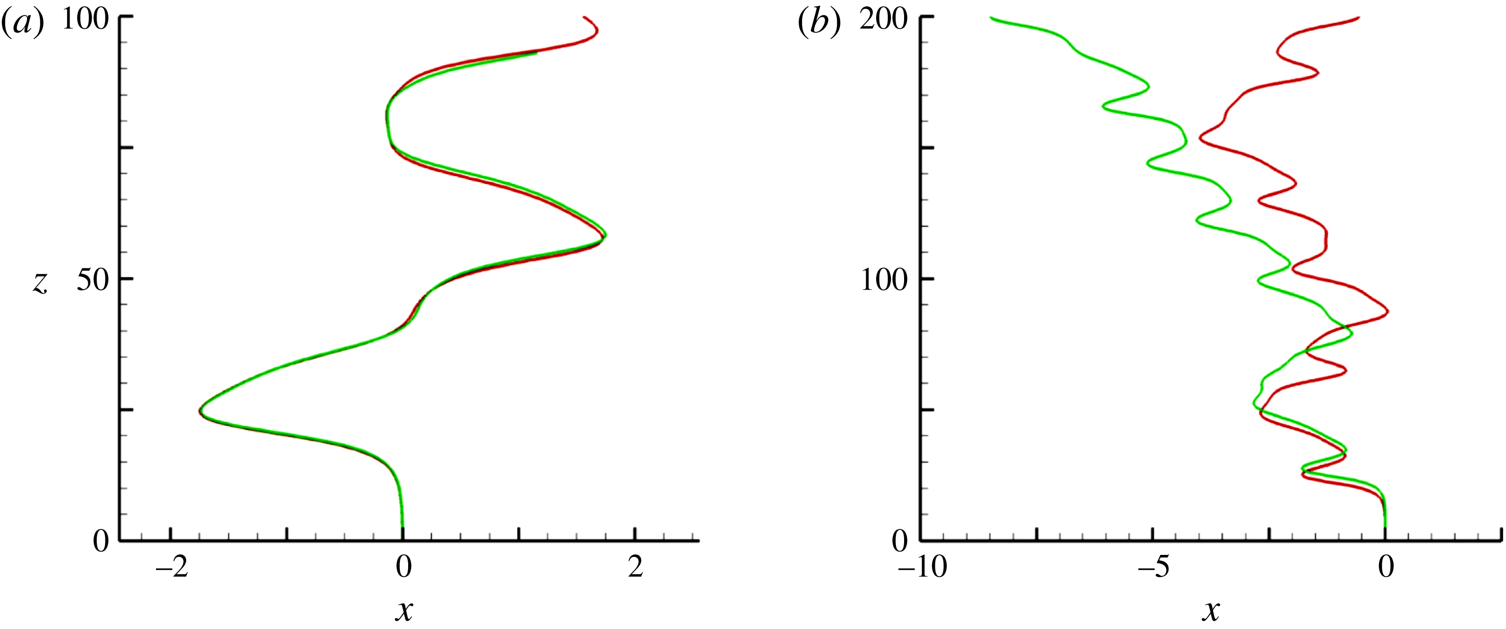
Figure 1. Paths of two spheres with the same
 $Ar$
but different
$Ar$
but different
 $\overline{\unicode[STIX]{x1D70C}}$
computed with (green curve) or without (red curve) the
$\overline{\unicode[STIX]{x1D70C}}$
computed with (green curve) or without (red curve) the
 $\unicode[STIX]{x1D6FF}$
-terms in (2.6)–(2.7) and the contribution
$\unicode[STIX]{x1D6FF}$
-terms in (2.6)–(2.7) and the contribution
 $\boldsymbol{u}^{\unicode[STIX]{x1D6FF}}$
in
$\boldsymbol{u}^{\unicode[STIX]{x1D6FF}}$
in
 $\boldsymbol{u}^{\prime }$
. (a)
$\boldsymbol{u}^{\prime }$
. (a)
 $\overline{\unicode[STIX]{x1D70C}}=0.33$
, (b)
$\overline{\unicode[STIX]{x1D70C}}=0.33$
, (b)
 $\overline{\unicode[STIX]{x1D70C}}=0.01$
; the horizontal (
$\overline{\unicode[STIX]{x1D70C}}=0.01$
; the horizontal (
 $x$
) and vertical (
$x$
) and vertical (
 $z$
) axes are normalized with the sphere diameter,
$z$
) axes are normalized with the sphere diameter,
 $d$
.
$d$
.
A typical example of the influence of viscous effects induced by the Stokes layer on the path evolution is shown in figure 1. The standard fluid/body coupling algorithm (Mougin & Magnaudet Reference Mougin and Magnaudet2002a
) and the modified version including the
 $\unicode[STIX]{x1D6FF}$
-terms in (2.6), (2.7) and the viscous contribution
$\unicode[STIX]{x1D6FF}$
-terms in (2.6), (2.7) and the viscous contribution
 $\boldsymbol{u}^{\unicode[STIX]{x1D6FF}}$
in
$\boldsymbol{u}^{\unicode[STIX]{x1D6FF}}$
in
 $\boldsymbol{u}^{\prime }$
produce virtually indiscernible results for the sphere with
$\boldsymbol{u}^{\prime }$
produce virtually indiscernible results for the sphere with
 $\overline{\unicode[STIX]{x1D70C}}=0.33$
. In contrast, the two algorithms predict dramatically different evolutions in the case of the very light sphere with
$\overline{\unicode[STIX]{x1D70C}}=0.33$
. In contrast, the two algorithms predict dramatically different evolutions in the case of the very light sphere with
 $\overline{\unicode[STIX]{x1D70C}}=0.01$
. This is fully in line with the analysis reported above: variations of the rotation rate in the former case are essentially governed by the sphere moment of inertia, while those in the latter case are controlled by the viscous torque associated with the unsteady diffusion of vorticity across the Stokes layer. This example clearly establishes that the path of very light spheres cannot be predicted without taking into account these subtle ‘history’ effects.
$\overline{\unicode[STIX]{x1D70C}}=0.01$
. This is fully in line with the analysis reported above: variations of the rotation rate in the former case are essentially governed by the sphere moment of inertia, while those in the latter case are controlled by the viscous torque associated with the unsteady diffusion of vorticity across the Stokes layer. This example clearly establishes that the path of very light spheres cannot be predicted without taking into account these subtle ‘history’ effects.
It is probably worth pointing out that the numerical strategy described in this section may easily be extended to bodies with more complex geometries, even though no closed-form expression is available for viscous (or even inviscid) effects due to the body acceleration. For this purpose, before running the complete problem, one simply needs to impose successively prescribed uniform translational or rotational accelerations to the body in each direction of space, record the evolutions of all force and torque components during a short time period and analyse them by using the methodology described in Rivero, Magnaudet & Fabre (Reference Rivero, Magnaudet and Fabre1991). This provides once and for all the whole set of coefficients involved in the counterpart of (2.6), (2.7).
2.3 Computational protocol
The fluid problem is spatially discretized on a spherical grid. Extensive tests were carried out to determine the grid characteristics, the goal being to guarantee grid-independent paths (which requires grid-independent loads on the sphere) while keeping the computational cost acceptable. The loads on the sphere are especially sensitive to the resolution of both the boundary layer and the near wake, and to the disturbances that may be generated by vortices leaving the computational domain through its outer boundary. Moreover, as the sphere freely moves, the wake may take any orientation with respect to the grid axis, which makes effects of the anisotropy inherent to the use of an axisymmetric grid of particular importance in the present problem. Last, since instabilities may act on short time scales, controlling the time step also requires specific attention. For these reasons, we very carefully considered the above five aspects. In appendix B, we detail the determination of the various grid parameters, discuss the condition that controls the time step, and summarize the results of several test cases.
Simulations to be described below were generally started from rest; nevertheless, to examine the influence of initial conditions, we also frequently ran computations for a given set of parameters by using fields
 $(\boldsymbol{U},P,\boldsymbol{V},\unicode[STIX]{x1D734})$
from a previous run corresponding to neighbouring values of
$(\boldsymbol{U},P,\boldsymbol{V},\unicode[STIX]{x1D734})$
from a previous run corresponding to neighbouring values of
 $Ar$
and
$Ar$
and
 $\overline{\unicode[STIX]{x1D70C}}$
. When starting from rest, a small disturbance was added during several time steps in the right-hand side of (2.6) to trigger the instability. Similarly, the stability of planar non-vertical paths was examined by introducing momentarily a small disturbance in the right-hand side of (2.6) and/or (2.7). In each run, the sphere was followed over a vertical distance ranging typically from
$\overline{\unicode[STIX]{x1D70C}}$
. When starting from rest, a small disturbance was added during several time steps in the right-hand side of (2.6) to trigger the instability. Similarly, the stability of planar non-vertical paths was examined by introducing momentarily a small disturbance in the right-hand side of (2.6) and/or (2.7). In each run, the sphere was followed over a vertical distance ranging typically from
 $250d$
to
$250d$
to
 $700d$
. To decide when a run was stopped, we combined different criteria, depending on the nature of the regime under consideration. Close to one of the first bifurcations of the system, we monitored the growth rate of the path deviations and stopped the computation once saturation was reached. In most cases we rather considered the various components of the force and torque acting on the sphere, and examined their variations. In particular, in periodic or quasi-periodic regimes, we stopped the computation when these changes were negligibly small (i.e. of the order of the computational accuracy expected on these dynamical quantities) over typically 10 periods. With the grid defined above, the CPU time of a typical run ranged from
$700d$
. To decide when a run was stopped, we combined different criteria, depending on the nature of the regime under consideration. Close to one of the first bifurcations of the system, we monitored the growth rate of the path deviations and stopped the computation once saturation was reached. In most cases we rather considered the various components of the force and torque acting on the sphere, and examined their variations. In particular, in periodic or quasi-periodic regimes, we stopped the computation when these changes were negligibly small (i.e. of the order of the computational accuracy expected on these dynamical quantities) over typically 10 periods. With the grid defined above, the CPU time of a typical run ranged from
 $500$
to
$500$
to
 $1000$
hours in sequential mode on a single-core PC.
$1000$
hours in sequential mode on a single-core PC.
3 Styles of paths and wakes
3.1 Preliminary comment
Before we discuss computational results, it is of interest to remark that some physical insight can be obtained directly from (2.6), (2.7) regarding the influence of the solid-to-fluid density ratio on the rise regimes. Indeed, the left-hand side of these equations involves three different types of contributions: those related to the body inertia, weighted by
 $\overline{\unicode[STIX]{x1D70C}}$
, those due to the fluid inertia, which in the present case reduce to the added-mass coefficient
$\overline{\unicode[STIX]{x1D70C}}$
, those due to the fluid inertia, which in the present case reduce to the added-mass coefficient
 $1/2$
in (2.6), and those resulting from the permanent existence of a Stokes layer around the sphere, due to the continual variations of its translational and rotational velocities. In the framework of the algorithm described above, the magnitude of the latter scales with the parameter
$1/2$
in (2.6), and those resulting from the permanent existence of a Stokes layer around the sphere, due to the continual variations of its translational and rotational velocities. In the framework of the algorithm described above, the magnitude of the latter scales with the parameter
 $\unicode[STIX]{x1D6FF}$
because the characteristic time involved in the time-advancement procedure is
$\unicode[STIX]{x1D6FF}$
because the characteristic time involved in the time-advancement procedure is
 $\unicode[STIX]{x0394}t$
. However, from a physical point of view, the relevant time scale is the gravitational time
$\unicode[STIX]{x0394}t$
. However, from a physical point of view, the relevant time scale is the gravitational time
 $t_{g}=d/V_{g}=\sqrt{d/((1-\overline{\unicode[STIX]{x1D70C}})g)}$
. Hence the influence of the Stokes layer on the body dynamics is measured by the dimensionless parameter
$t_{g}=d/V_{g}=\sqrt{d/((1-\overline{\unicode[STIX]{x1D70C}})g)}$
. Hence the influence of the Stokes layer on the body dynamics is measured by the dimensionless parameter
 $\unicode[STIX]{x0394}=(\unicode[STIX]{x1D708}t_{g}/d^{2})^{1/2}=Ar^{-1/2}$
. Based on the comparison of the three characteristic orders of magnitude
$\unicode[STIX]{x0394}=(\unicode[STIX]{x1D708}t_{g}/d^{2})^{1/2}=Ar^{-1/2}$
. Based on the comparison of the three characteristic orders of magnitude
 $\overline{\unicode[STIX]{x1D70C}},1/2$
and
$\overline{\unicode[STIX]{x1D70C}},1/2$
and
 $Ar^{-1/2}$
, one may anticipate three different classes of dynamical regimes, keeping in mind that
$Ar^{-1/2}$
, one may anticipate three different classes of dynamical regimes, keeping in mind that
 $Ar^{-1/2}\ll 1$
: those of ‘heavy’ spheres corresponding to
$Ar^{-1/2}\ll 1$
: those of ‘heavy’ spheres corresponding to
 $\overline{\unicode[STIX]{x1D70C}}\gg 1/2$
(here presumably restricted to
$\overline{\unicode[STIX]{x1D70C}}\gg 1/2$
(here presumably restricted to
 $\overline{\unicode[STIX]{x1D70C}}\lesssim 1$
), those of spheres with intermediate density ratios such that
$\overline{\unicode[STIX]{x1D70C}}\lesssim 1$
), those of spheres with intermediate density ratios such that
 $(1/2)\gg \overline{\unicode[STIX]{x1D70C}}\gg Ar^{-1/2}$
, and those of very light spheres with
$(1/2)\gg \overline{\unicode[STIX]{x1D70C}}\gg Ar^{-1/2}$
, and those of very light spheres with
 $\overline{\unicode[STIX]{x1D70C}}\ll Ar^{-1/2}$
(here
$\overline{\unicode[STIX]{x1D70C}}\ll Ar^{-1/2}$
(here
 $0.04\leqslant Ar^{-1/2}\leqslant 0.08$
). In the first regime, possible changes in the translational and rotational sphere velocities are entirely driven by quasi-steady hydrodynamic stresses and body inertia. In contrast, in the second case, fluid acceleration plays a dominant role in the translational dynamics, while changes in the rotation rate are still controlled by the sphere moment of inertia. Last, in the regime
$0.04\leqslant Ar^{-1/2}\leqslant 0.08$
). In the first regime, possible changes in the translational and rotational sphere velocities are entirely driven by quasi-steady hydrodynamic stresses and body inertia. In contrast, in the second case, fluid acceleration plays a dominant role in the translational dynamics, while changes in the rotation rate are still controlled by the sphere moment of inertia. Last, in the regime
 $\overline{\unicode[STIX]{x1D70C}}\ll Ar^{-1/2}$
, the fluid also controls the rotational dynamics through the viscous processes involved in the Stokes layer. Of course intermediate regimes are expected to take place for
$\overline{\unicode[STIX]{x1D70C}}\ll Ar^{-1/2}$
, the fluid also controls the rotational dynamics through the viscous processes involved in the Stokes layer. Of course intermediate regimes are expected to take place for
 $\overline{\unicode[STIX]{x1D70C}}\approx 1/2$
and
$\overline{\unicode[STIX]{x1D70C}}\approx 1/2$
and
 $\overline{\unicode[STIX]{x1D70C}}\approx Ar^{-1/2}$
, where the body and fluid both drive the translational and rotational dynamics, respectively. The findings described in the rest of this paper will confirm the above analysis, especially the strikingly distinct behaviour of ‘heavy’ and ‘very light’ spheres in several ranges of
$\overline{\unicode[STIX]{x1D70C}}\approx Ar^{-1/2}$
, where the body and fluid both drive the translational and rotational dynamics, respectively. The findings described in the rest of this paper will confirm the above analysis, especially the strikingly distinct behaviour of ‘heavy’ and ‘very light’ spheres in several ranges of
 $Ar$
. Note that the dividing density ratio
$Ar$
. Note that the dividing density ratio
 $\overline{\unicode[STIX]{x1D70C}}=1$
separating falling and rising spheres does not play any role in the above classification. Hence spheres with
$\overline{\unicode[STIX]{x1D70C}}=1$
separating falling and rising spheres does not play any role in the above classification. Hence spheres with
 $\overline{\unicode[STIX]{x1D70C}}\gtrsim 1$
(which are not considered here) and with
$\overline{\unicode[STIX]{x1D70C}}\gtrsim 1$
(which are not considered here) and with
 $\overline{\unicode[STIX]{x1D70C}}\lesssim 1$
are expected to behave similarly. This is indeed what was observed by ZD. Obviously the above classification only makes sense in unsteady regimes, since the sphere inertia does not play any role as far as the translational and rotational velocities do not change over time.
$\overline{\unicode[STIX]{x1D70C}}\lesssim 1$
are expected to behave similarly. This is indeed what was observed by ZD. Obviously the above classification only makes sense in unsteady regimes, since the sphere inertia does not play any role as far as the translational and rotational velocities do not change over time.
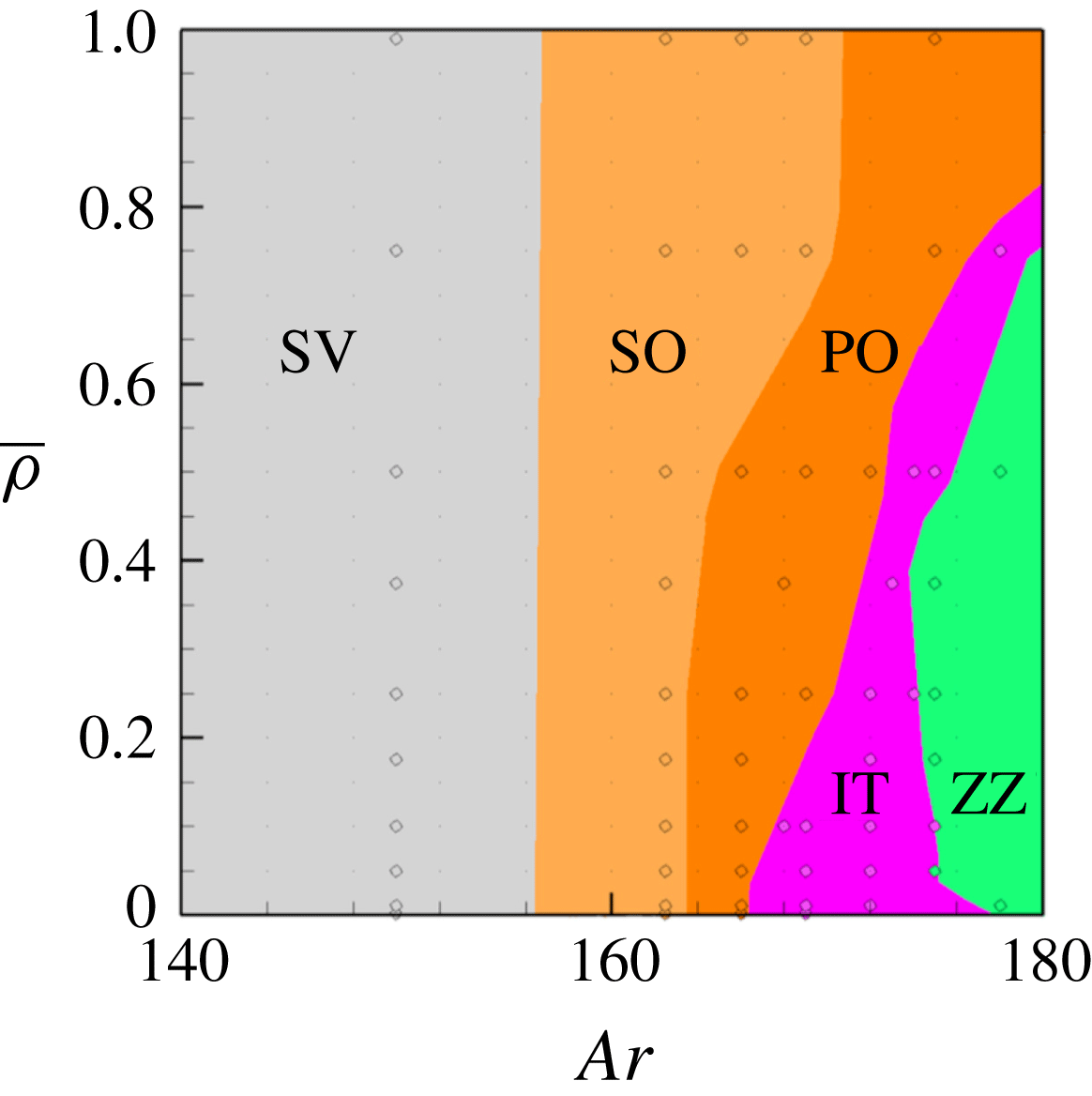
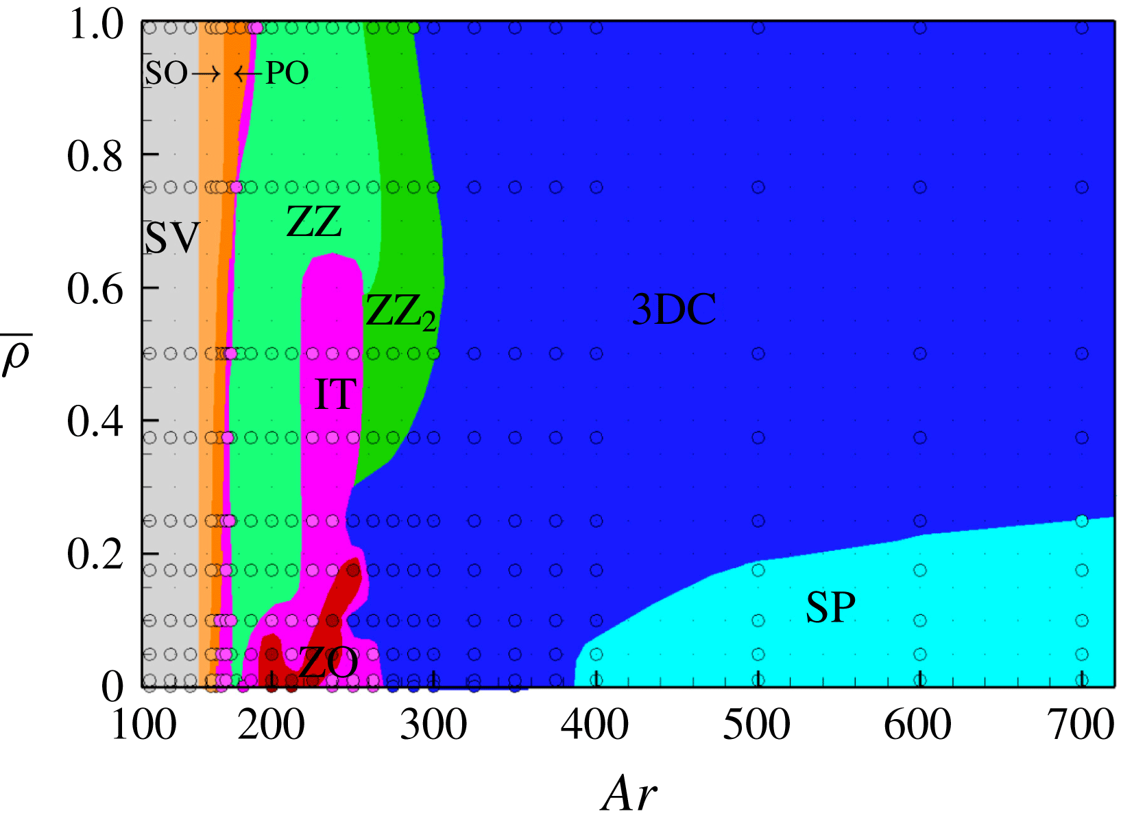
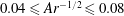
Figure 2. State diagram of the first rise regimes in the range
 $140\leqslant Ar\leqslant 180$
. Grey: steady vertical (SV); pale orange: steady oblique (SO); dark orange: periodic oblique (PO); purple: intermittent (IT); green: large-amplitude zigzagging (ZZ).
$140\leqslant Ar\leqslant 180$
. Grey: steady vertical (SV); pale orange: steady oblique (SO); dark orange: periodic oblique (PO); purple: intermittent (IT); green: large-amplitude zigzagging (ZZ).
3.2 First non-vertical regimes
Figure 2 gathers the various regimes of rise observed up to
 $Ar=180$
. Starting from left, i.e. from low
$Ar=180$
. Starting from left, i.e. from low
 $Ar$
, the first encountered regime corresponds of course to a steady vertical (SV) rise associated with an axisymmetric flow field. Increasing
$Ar$
, the first encountered regime corresponds of course to a steady vertical (SV) rise associated with an axisymmetric flow field. Increasing
 $Ar$
, this base state is succeeded by a steady oblique (SO) regime which was first identified numerically by JDB before it was unambiguously observed experimentally by Veldhuis & Biesheuvel (Reference Veldhuis and Biesheuvel2007) and Horowitz & Williamson (Reference Horowitz and Williamson2010). Somewhat later, the SV–SO transition was shown to correspond to a stationary (pitchfork) bifurcation by Fabre, Tchoufag & Magnaudet (Reference Fabre, Tchoufag and Magnaudet2012). The same study determined that the corresponding threshold takes place at
$Ar$
, this base state is succeeded by a steady oblique (SO) regime which was first identified numerically by JDB before it was unambiguously observed experimentally by Veldhuis & Biesheuvel (Reference Veldhuis and Biesheuvel2007) and Horowitz & Williamson (Reference Horowitz and Williamson2010). Somewhat later, the SV–SO transition was shown to correspond to a stationary (pitchfork) bifurcation by Fabre, Tchoufag & Magnaudet (Reference Fabre, Tchoufag and Magnaudet2012). The same study determined that the corresponding threshold takes place at
 $Ar=155.6$
, irrespective of the sphere-to-fluid density ratio. The recent computations reported in ZD confirmed this threshold and its remarkable independence with respect to
$Ar=155.6$
, irrespective of the sphere-to-fluid density ratio. The recent computations reported in ZD confirmed this threshold and its remarkable independence with respect to
 $\overline{\unicode[STIX]{x1D70C}}$
which is also in line with the qualitative analysis developed above. Here, since we are essentially interested in time-dependent regimes, we did not attempt to recover precisely this threshold throughout the whole range of
$\overline{\unicode[STIX]{x1D70C}}$
which is also in line with the qualitative analysis developed above. Here, since we are essentially interested in time-dependent regimes, we did not attempt to recover precisely this threshold throughout the whole range of
 $\overline{\unicode[STIX]{x1D70C}}$
; hence in figure 2, the vertical line separating the SV and SO regimes is merely based on the prediction of Fabre et al. (Reference Fabre, Tchoufag and Magnaudet2012). Nevertheless some specific runs allowed us to observe that the SV–SO threshold stands in the range
$\overline{\unicode[STIX]{x1D70C}}$
; hence in figure 2, the vertical line separating the SV and SO regimes is merely based on the prediction of Fabre et al. (Reference Fabre, Tchoufag and Magnaudet2012). Nevertheless some specific runs allowed us to observe that the SV–SO threshold stands in the range
 $155<Ar<156$
for small
$155<Ar<156$
for small
 $\overline{\unicode[STIX]{x1D70C}}$
as well as for
$\overline{\unicode[STIX]{x1D70C}}$
as well as for
 $\overline{\unicode[STIX]{x1D70C}}=0.99$
, in line with this prediction; we also checked that the system is still in the SV regime for
$\overline{\unicode[STIX]{x1D70C}}=0.99$
, in line with this prediction; we also checked that the system is still in the SV regime for
 $Ar=150$
whatever
$Ar=150$
whatever
 $\overline{\unicode[STIX]{x1D70C}}$
, whereas it is always in the SO regime when
$\overline{\unicode[STIX]{x1D70C}}$
, whereas it is always in the SO regime when
 $Ar=162.5$
. Moreover, as figure 3 reveals, the sphere rotation rate and drift angle are still independent of
$Ar=162.5$
. Moreover, as figure 3 reveals, the sphere rotation rate and drift angle are still independent of
 $\overline{\unicode[STIX]{x1D70C}}$
for
$\overline{\unicode[STIX]{x1D70C}}$
for
 $Ar=162.5$
(i.e. they only depend on the distance to the threshold), the drift angle with respect to the
$Ar=162.5$
(i.e. they only depend on the distance to the threshold), the drift angle with respect to the
 $z$
-axis being approximately
$z$
-axis being approximately
 $4.3^{\circ }$
(throughout the paper,
$4.3^{\circ }$
(throughout the paper,
 $z$
denotes the vertical ascending coordinate and
$z$
denotes the vertical ascending coordinate and
 $x$
and
$x$
and
 $y$
lie in the horizontal plane; all three coordinates are normalized by
$y$
lie in the horizontal plane; all three coordinates are normalized by
 $d$
). On the same figure, one may also notice that the vertical position at which the SV–SO transition takes place slightly increases as
$d$
). On the same figure, one may also notice that the vertical position at which the SV–SO transition takes place slightly increases as
 $\overline{\unicode[STIX]{x1D70C}}$
decreases (compare the green and orange curves). However, one has to keep in mind that the terminal rise velocity resulting from the balance between drag and buoyancy forces roughly varies as
$\overline{\unicode[STIX]{x1D70C}}$
decreases (compare the green and orange curves). However, one has to keep in mind that the terminal rise velocity resulting from the balance between drag and buoyancy forces roughly varies as
 $(1-\overline{\unicode[STIX]{x1D70C}})^{1/2}$
since the flow is dominated by inertia effects (
$(1-\overline{\unicode[STIX]{x1D70C}})^{1/2}$
since the flow is dominated by inertia effects (
 $Ar\gg 1$
). Hence, the time at which the transition takes place is actually approximately one order of magnitude smaller for the lightest spheres than for the heaviest ones. This is consistent with the fact that the smaller the sphere inertia, the larger the rate of change of the sphere velocity and rotation rate in response to a given force or torque disturbance, hence the faster the transition.
$Ar\gg 1$
). Hence, the time at which the transition takes place is actually approximately one order of magnitude smaller for the lightest spheres than for the heaviest ones. This is consistent with the fact that the smaller the sphere inertia, the larger the rate of change of the sphere velocity and rotation rate in response to a given force or torque disturbance, hence the faster the transition.

Figure 3. Paths for various solid-to-fluid density ratios at
 $Ar=162.5$
(SO regime). From top to bottom:
$Ar=162.5$
(SO regime). From top to bottom:
 $\overline{\unicode[STIX]{x1D70C}}=0.001$
(red, almost hidden under the green curve),
$\overline{\unicode[STIX]{x1D70C}}=0.001$
(red, almost hidden under the green curve),
 $0.01$
(green),
$0.01$
(green),
 $0.05$
(blue),
$0.05$
(blue),
 $0.1$
(purple),
$0.1$
(purple),
 $0.25$
(cyan),
$0.25$
(cyan),
 $0.5$
(yellow),
$0.5$
(yellow),
 $0.75$
(black),
$0.75$
(black),
 $0.99$
(orange).
$0.99$
(orange).
Increasing
 $Ar$
, the SO regime is quickly replaced by a periodic oscillating (PO) regime. The threshold of the corresponding transition increases with
$Ar$
, the SO regime is quickly replaced by a periodic oscillating (PO) regime. The threshold of the corresponding transition increases with
 $\overline{\unicode[STIX]{x1D70C}}$
, from
$\overline{\unicode[STIX]{x1D70C}}$
, from
 $164.4$
for
$164.4$
for
 $\overline{\unicode[STIX]{x1D70C}}\approx 0$
to
$\overline{\unicode[STIX]{x1D70C}}\approx 0$
to
 $173.3$
for
$173.3$
for
 $\overline{\unicode[STIX]{x1D70C}}\approx 1$
. These values are slightly smaller than those reported by ZD (167.2 and 178.5, respectively). The PO regime is only observed up to
$\overline{\unicode[STIX]{x1D70C}}\approx 1$
. These values are slightly smaller than those reported by ZD (167.2 and 178.5, respectively). The PO regime is only observed up to
 $Ar=167.3$
when
$Ar=167.3$
when
 $\overline{\unicode[STIX]{x1D70C}}\approx 0$
; this upper limit increases with
$\overline{\unicode[STIX]{x1D70C}}\approx 0$
; this upper limit increases with
 $\overline{\unicode[STIX]{x1D70C}}$
(mostly for
$\overline{\unicode[STIX]{x1D70C}}$
(mostly for
 $\overline{\unicode[STIX]{x1D70C}}>0.5$
), up to
$\overline{\unicode[STIX]{x1D70C}}>0.5$
), up to
 $Ar=187.7$
when
$Ar=187.7$
when
 $\overline{\unicode[STIX]{x1D70C}}\approx 1$
. Whatever
$\overline{\unicode[STIX]{x1D70C}}\approx 1$
. Whatever
 $\overline{\unicode[STIX]{x1D70C}}$
, the dimensionless frequency (or Strouhal number) is approximately 0.045 at the SO–PO threshold and decreases with the distance to the threshold. This finding is in good agreement with the results of ZD that indicate values of
$\overline{\unicode[STIX]{x1D70C}}$
, the dimensionless frequency (or Strouhal number) is approximately 0.045 at the SO–PO threshold and decreases with the distance to the threshold. This finding is in good agreement with the results of ZD that indicate values of
 $St$
close to 0.05 at the SO–PO threshold throughout the density ratio range
$St$
close to 0.05 at the SO–PO threshold throughout the density ratio range
 $0\leqslant \overline{\unicode[STIX]{x1D70C}}\leqslant 2$
. Compared with usual Strouhal numbers associated with vortex shedding in bluff-body wakes, the values involved here are typically 3–4 times smaller, revealing a low-frequency oscillation. To better understand this feature, it is important to realize that the sphere average Reynolds number,
$0\leqslant \overline{\unicode[STIX]{x1D70C}}\leqslant 2$
. Compared with usual Strouhal numbers associated with vortex shedding in bluff-body wakes, the values involved here are typically 3–4 times smaller, revealing a low-frequency oscillation. To better understand this feature, it is important to realize that the sphere average Reynolds number,
 $Re_{m}$
, is in the range [220, 255] throughout the range of
$Re_{m}$
, is in the range [220, 255] throughout the range of
 $Ar$
within which the PO regime is observed. Hence, no vortex shedding would take place in the wake, were the sphere forced to rise in straight line, since the onset of vortex shedding past a sphere held fixed in a uniform stream corresponds to a critical Reynolds number of approximately 275 (Ghidersa & Dušek Reference Ghidersa and Dušek2000). Therefore the observed low-frequency path oscillation unambiguously results from the couplings of the sphere dynamics and the surrounding flow. This is similar to what is for instance observed with disks which, in some ranges of
$Ar$
within which the PO regime is observed. Hence, no vortex shedding would take place in the wake, were the sphere forced to rise in straight line, since the onset of vortex shedding past a sphere held fixed in a uniform stream corresponds to a critical Reynolds number of approximately 275 (Ghidersa & Dušek Reference Ghidersa and Dušek2000). Therefore the observed low-frequency path oscillation unambiguously results from the couplings of the sphere dynamics and the surrounding flow. This is similar to what is for instance observed with disks which, in some ranges of
 $\overline{\unicode[STIX]{x1D70C}}$
, start fluttering at a critical Reynolds number much lower than the threshold corresponding to the loss of axisymmetry in the wake of a disk held fixed in a uniform flow (Auguste et al.
Reference Auguste, Magnaudet and Fabre2013). Figure 4 shows a typical PO path, together with the associated wake evolution observed through the
$\overline{\unicode[STIX]{x1D70C}}$
, start fluttering at a critical Reynolds number much lower than the threshold corresponding to the loss of axisymmetry in the wake of a disk held fixed in a uniform flow (Auguste et al.
Reference Auguste, Magnaudet and Fabre2013). Figure 4 shows a typical PO path, together with the associated wake evolution observed through the
 $\unicode[STIX]{x1D706}_{2}$
criterion (Jeong & Hussain Reference Jeong and Hussain1995). The path inclination oscillates from
$\unicode[STIX]{x1D706}_{2}$
criterion (Jeong & Hussain Reference Jeong and Hussain1995). The path inclination oscillates from
 $2.6^{\circ }$
to
$2.6^{\circ }$
to
 $7.3^{\circ }$
, with an average value of approximately
$7.3^{\circ }$
, with an average value of approximately
 $4.5^{\circ }$
. As the correspondence between the path and wake reveals, the streamwise vortex pair is virtually absent when the path is almost vertical (stage 1), and the larger the inclination the more intense this vortex pair, with a maximum during stages 2 and 4. This is no surprise since streamwise vortices are responsible for the lift force acting on the sphere, which is the cause of the bending of its path. Similar to the SO regime, the sign of the streamwise vorticity remains constant within each thread, which yields the non-zero average horizontal drift of the trajectory.
$4.5^{\circ }$
. As the correspondence between the path and wake reveals, the streamwise vortex pair is virtually absent when the path is almost vertical (stage 1), and the larger the inclination the more intense this vortex pair, with a maximum during stages 2 and 4. This is no surprise since streamwise vortices are responsible for the lift force acting on the sphere, which is the cause of the bending of its path. Similar to the SO regime, the sign of the streamwise vorticity remains constant within each thread, which yields the non-zero average horizontal drift of the trajectory.

Figure 4. Characteristics of the PO regime for
 $\overline{\unicode[STIX]{x1D70C}}=0.5$
and
$\overline{\unicode[STIX]{x1D70C}}=0.5$
and
 $Ar=172$
. (a) Sphere trajectory; (b) wake evolution during about
$Ar=172$
. (a) Sphere trajectory; (b) wake evolution during about
 $3/4$
of a period; the wake is visualized using the
$3/4$
of a period; the wake is visualized using the
 $\unicode[STIX]{x1D706}_{2}$
criterion (Jeong & Hussain Reference Jeong and Hussain1995), with iso-
$\unicode[STIX]{x1D706}_{2}$
criterion (Jeong & Hussain Reference Jeong and Hussain1995), with iso-
 $\unicode[STIX]{x1D706}_{2}$
surfaces coloured by the local value of the vertical component,
$\unicode[STIX]{x1D706}_{2}$
surfaces coloured by the local value of the vertical component,
 $\unicode[STIX]{x1D714}_{z}$
, of the vorticity normalized by
$\unicode[STIX]{x1D714}_{z}$
, of the vorticity normalized by
 $V_{g}/d$
(
$V_{g}/d$
(
 $-1.94\leqslant \unicode[STIX]{x1D714}_{z}\leqslant 1.94$
,
$-1.94\leqslant \unicode[STIX]{x1D714}_{z}\leqslant 1.94$
,
 $\unicode[STIX]{x1D714}_{z}\approx 0$
in green regions).
$\unicode[STIX]{x1D714}_{z}\approx 0$
in green regions).
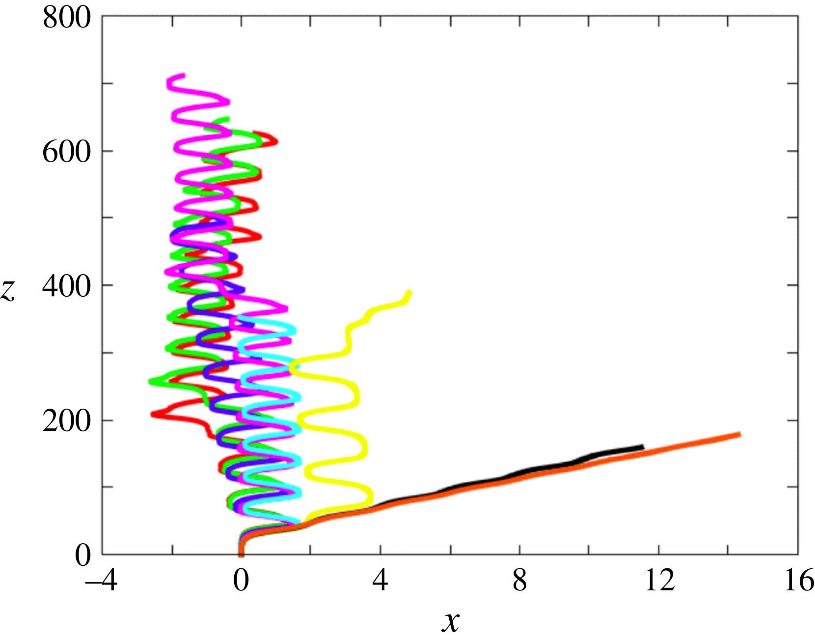
Figure 5. Paths for various solid-to-fluid density ratios at
 $Ar=175$
. Same colour code as in figure 3.
$Ar=175$
. Same colour code as in figure 3.
Throughout the whole range of
 $\overline{\unicode[STIX]{x1D70C}}$
, the PO regime is succeeded by an intermittent regime within which the sphere ‘hesitates’ more or less often to perform periodic planar zigzags. That is, it drifts laterally for a while until its path becomes nearly vertical. At this point, it either starts to drift in the opposite direction, then performing a full zigzag, or does not succeed to do so, then keeping on drifting in the same direction, possibly in a different vertical plane. Indeed, since ‘hesitations’ take place during the time lapse when the wake is almost axisymmetric (as in stage 1 of figure 4), the system is momentarily free to select a new symmetry plane. This succession of ‘successes’ and ‘failures’ in performing complete zigzags occurs randomly. Such rare events are known to be characteristic of intermittency in dynamical systems and transition to turbulence (Manneville & Pomeau Reference Manneville and Pomeau1979; Pomeau & Manneville Reference Pomeau and Manneville1980; Bergé, Pomeau & Vidal Reference Bergé, Pomeau and Vidal1984). Hence this new regime, which we refer to as IT, marks the onset of chaos in the present dynamical system whatever
$\overline{\unicode[STIX]{x1D70C}}$
, the PO regime is succeeded by an intermittent regime within which the sphere ‘hesitates’ more or less often to perform periodic planar zigzags. That is, it drifts laterally for a while until its path becomes nearly vertical. At this point, it either starts to drift in the opposite direction, then performing a full zigzag, or does not succeed to do so, then keeping on drifting in the same direction, possibly in a different vertical plane. Indeed, since ‘hesitations’ take place during the time lapse when the wake is almost axisymmetric (as in stage 1 of figure 4), the system is momentarily free to select a new symmetry plane. This succession of ‘successes’ and ‘failures’ in performing complete zigzags occurs randomly. Such rare events are known to be characteristic of intermittency in dynamical systems and transition to turbulence (Manneville & Pomeau Reference Manneville and Pomeau1979; Pomeau & Manneville Reference Pomeau and Manneville1980; Bergé, Pomeau & Vidal Reference Bergé, Pomeau and Vidal1984). Hence this new regime, which we refer to as IT, marks the onset of chaos in the present dynamical system whatever
 $\overline{\unicode[STIX]{x1D70C}}$
(its chaotic nature will be established later). The IT regime covers only a narrow parameter range, from 2 to 10
$\overline{\unicode[STIX]{x1D70C}}$
(its chaotic nature will be established later). The IT regime covers only a narrow parameter range, from 2 to 10
 $Ar$
-units depending on
$Ar$
-units depending on
 $\overline{\unicode[STIX]{x1D70C}}$
, the narrowest part being found in the range
$\overline{\unicode[STIX]{x1D70C}}$
, the narrowest part being found in the range
 $0.3\leqslant \overline{\unicode[STIX]{x1D70C}}\leqslant 0.75$
. The styles of path observed in this intermittent regime and the influence of the sphere-to-fluid density ratio on the PO–IT transition may be appreciated in figure 5 which corresponds to
$0.3\leqslant \overline{\unicode[STIX]{x1D70C}}\leqslant 0.75$
. The styles of path observed in this intermittent regime and the influence of the sphere-to-fluid density ratio on the PO–IT transition may be appreciated in figure 5 which corresponds to
 $Ar=175$
. Starting from
$Ar=175$
. Starting from
 $\overline{\unicode[STIX]{x1D70C}}\approx 1$
, the two heaviest spheres are still in the PO regime, the amplitude of oscillations increasing when
$\overline{\unicode[STIX]{x1D70C}}\approx 1$
, the two heaviest spheres are still in the PO regime, the amplitude of oscillations increasing when
 $\overline{\unicode[STIX]{x1D70C}}$
decreases. For
$\overline{\unicode[STIX]{x1D70C}}$
decreases. For
 $\overline{\unicode[STIX]{x1D70C}}=0.5$
, the sphere first describes several complete zigzags until its horizontal velocity fails to reverse. Then it starts to drift along an inclined path reminiscent of those observed in the PO regime. In the range
$\overline{\unicode[STIX]{x1D70C}}=0.5$
, the sphere first describes several complete zigzags until its horizontal velocity fails to reverse. Then it starts to drift along an inclined path reminiscent of those observed in the PO regime. In the range
 $0.25\leqslant \overline{\unicode[STIX]{x1D70C}}\leqslant 0.05$
, the paths consist essentially of periodic zigzags. However a ‘failure’ still occurs after the sphere has travelled a vertical distance of
$0.25\leqslant \overline{\unicode[STIX]{x1D70C}}\leqslant 0.05$
, the paths consist essentially of periodic zigzags. However a ‘failure’ still occurs after the sphere has travelled a vertical distance of
 $O(350d)$
for
$O(350d)$
for
 $\overline{\unicode[STIX]{x1D70C}}=0.1$
; no such feature is observed for
$\overline{\unicode[STIX]{x1D70C}}=0.1$
; no such feature is observed for
 $\overline{\unicode[STIX]{x1D70C}}=0.25$
and
$\overline{\unicode[STIX]{x1D70C}}=0.25$
and
 $0.05$
throughout the entire ascent, although there is no guarantee that it would not occur at a higher vertical position; one may also notice that a significant average drift exists in the latter case. The lightest two spheres exhibit a somewhat different behaviour: throughout their ascent, their paths follow complete zigzags, but in the late stage one of these zigzags is asymmetric, i.e. the sphere spends a longer time drifting in one direction than in the other, making the average path suddenly exhibit a slight lateral shift. This may be interpreted as a weak form of the above defect: the horizontal velocity does not change sign in due time to maintain the strict periodicity of the zigzag; however, it succeeds to do so with some limited delay, keeping the appearance of the path close to that of a pure zigzag (as will be shown in figure 10, slightly increasing the Archimedes number up to
$0.05$
throughout the entire ascent, although there is no guarantee that it would not occur at a higher vertical position; one may also notice that a significant average drift exists in the latter case. The lightest two spheres exhibit a somewhat different behaviour: throughout their ascent, their paths follow complete zigzags, but in the late stage one of these zigzags is asymmetric, i.e. the sphere spends a longer time drifting in one direction than in the other, making the average path suddenly exhibit a slight lateral shift. This may be interpreted as a weak form of the above defect: the horizontal velocity does not change sign in due time to maintain the strict periodicity of the zigzag; however, it succeeds to do so with some limited delay, keeping the appearance of the path close to that of a pure zigzag (as will be shown in figure 10, slightly increasing the Archimedes number up to
 $Ar=178$
yields a strictly periodic zigzagging path for
$Ar=178$
yields a strictly periodic zigzagging path for
 $\overline{\unicode[STIX]{x1D70C}}=0.01$
). Overall, what can be concluded from this sequence is that the smaller
$\overline{\unicode[STIX]{x1D70C}}=0.01$
). Overall, what can be concluded from this sequence is that the smaller
 $\overline{\unicode[STIX]{x1D70C}}$
, the less intermittent the sphere dynamics at this particular value of
$\overline{\unicode[STIX]{x1D70C}}$
, the less intermittent the sphere dynamics at this particular value of
 $Ar$
. In contrast, as soon as the sphere trajectory is essentially made of zigzags, the amplitude of the latter is almost independent of
$Ar$
. In contrast, as soon as the sphere trajectory is essentially made of zigzags, the amplitude of the latter is almost independent of
 $\overline{\unicode[STIX]{x1D70C}}$
and is about one sphere diameter.
$\overline{\unicode[STIX]{x1D70C}}$
and is about one sphere diameter.
3.3 Periodic and intermittent regimes up to
 $Ar=300$

As figure 6(a) shows, the situation changes significantly when
 $Ar$
is increased up to
$Ar$
is increased up to
 $187.5$
. The heaviest sphere is still in the PO regime with an average drift angle similar to that previously found (
$187.5$
. The heaviest sphere is still in the PO regime with an average drift angle similar to that previously found (
 $4.2^{\circ }$
); however path oscillations are now highly asymmetric. All spheres corresponding to
$4.2^{\circ }$
); however path oscillations are now highly asymmetric. All spheres corresponding to
 $0.1\leqslant \overline{\unicode[STIX]{x1D70C}}\leqslant 0.75$
exhibit regular planar zigzagging paths, demonstrating the existence of a well-defined periodic ZZ (zigzagging) regime. The amplitude of the corresponding lateral excursions is still of
$0.1\leqslant \overline{\unicode[STIX]{x1D70C}}\leqslant 0.75$
exhibit regular planar zigzagging paths, demonstrating the existence of a well-defined periodic ZZ (zigzagging) regime. The amplitude of the corresponding lateral excursions is still of
 $O(d)$
and slightly increases when
$O(d)$
and slightly increases when
 $\overline{\unicode[STIX]{x1D70C}}$
decreases; one may also notice a weak average drift showing no clear trend with
$\overline{\unicode[STIX]{x1D70C}}$
decreases; one may also notice a weak average drift showing no clear trend with
 $\overline{\unicode[STIX]{x1D70C}}$
(this drift is almost zero for
$\overline{\unicode[STIX]{x1D70C}}$
(this drift is almost zero for
 $\overline{\unicode[STIX]{x1D70C}}=0.5$
). As
$\overline{\unicode[STIX]{x1D70C}}=0.5$
). As
 $\overline{\unicode[STIX]{x1D70C}}$
is decreased, the zigzags become more and more nonlinear, higher harmonics contributing to make their extremities sharper. For
$\overline{\unicode[STIX]{x1D70C}}$
is decreased, the zigzags become more and more nonlinear, higher harmonics contributing to make their extremities sharper. For
 $\overline{\unicode[STIX]{x1D70C}}=0.1$
, a slight lateral shift of the uppermost zigzag may be discerned, suggesting that the corresponding conditions are close to the transition between a strictly periodic regime and an intermittent one. This is confirmed by the evolution of the paths observed with the lightest three spheres which exhibit erratic, albeit still planar, paths (the ratio of the out-of-plane to in-plane lateral displacements is
$\overline{\unicode[STIX]{x1D70C}}=0.1$
, a slight lateral shift of the uppermost zigzag may be discerned, suggesting that the corresponding conditions are close to the transition between a strictly periodic regime and an intermittent one. This is confirmed by the evolution of the paths observed with the lightest three spheres which exhibit erratic, albeit still planar, paths (the ratio of the out-of-plane to in-plane lateral displacements is
 ${\leqslant}5\times 10^{-5}$
). The various styles of path encountered in figure 6(a) provide a clear illustration of the three distinct behaviours predicted on the basis of the qualitative analysis presented in § 3.1, with one PO path for
${\leqslant}5\times 10^{-5}$
). The various styles of path encountered in figure 6(a) provide a clear illustration of the three distinct behaviours predicted on the basis of the qualitative analysis presented in § 3.1, with one PO path for
 $\overline{\unicode[STIX]{x1D70C}}\lesssim 1$
, several intermittent paths for
$\overline{\unicode[STIX]{x1D70C}}\lesssim 1$
, several intermittent paths for
 $\overline{\unicode[STIX]{x1D70C}}\lesssim Ar^{-1/2}$
(here
$\overline{\unicode[STIX]{x1D70C}}\lesssim Ar^{-1/2}$
(here
 $Ar^{-1/2}=0.073$
), and periodic ZZ paths in between.
$Ar^{-1/2}=0.073$
), and periodic ZZ paths in between.
Figure 6. Paths for various solid-to-fluid density ratios at (a)
 $Ar=187.5$
and (b)
$Ar=187.5$
and (b)
 $Ar=200$
:
$Ar=200$
:
 $\overline{\unicode[STIX]{x1D70C}}=0.001$
(red),
$\overline{\unicode[STIX]{x1D70C}}=0.001$
(red),
 $0.01$
(green),
$0.01$
(green),
 $0.05$
(blue),
$0.05$
(blue),
 $0.1$
(purple),
$0.1$
(purple),
 $0.175$
(grey),
$0.175$
(grey),
 $0.25$
(cyan),
$0.25$
(cyan),
 $0.5$
(yellow),
$0.5$
(yellow),
 $0.75$
(black),
$0.75$
(black),
 $0.99$
(orange).
$0.99$
(orange).
Increasing further
 $Ar$
up to
$Ar$
up to
 $200$
leads to a simpler situation, with essentially two styles of periodic paths (figure 6
b). Spheres with
$200$
leads to a simpler situation, with essentially two styles of periodic paths (figure 6
b). Spheres with
 $\overline{\unicode[STIX]{x1D70C}}\geqslant 0.175$
are found to follow well-defined zigzagging trajectories; their characteristics and variations with
$\overline{\unicode[STIX]{x1D70C}}\geqslant 0.175$
are found to follow well-defined zigzagging trajectories; their characteristics and variations with
 $\overline{\unicode[STIX]{x1D70C}}$
are similar to those described above. In contrast, very light spheres with
$\overline{\unicode[STIX]{x1D70C}}$
are similar to those described above. In contrast, very light spheres with
 $\overline{\unicode[STIX]{x1D70C}}\leqslant 0.05$
follow a new type of periodic path combining characteristic features of PO and ZZ paths. More precisely, the corresponding trajectories exhibit a clear lateral drift (about
$\overline{\unicode[STIX]{x1D70C}}\leqslant 0.05$
follow a new type of periodic path combining characteristic features of PO and ZZ paths. More precisely, the corresponding trajectories exhibit a clear lateral drift (about
 $3^{\circ }$
for the lightest sphere, then decreasing with increasing
$3^{\circ }$
for the lightest sphere, then decreasing with increasing
 $\overline{\unicode[STIX]{x1D70C}}$
) but the oscillations are much more pronounced than in the PO regime, the horizontal velocity being able to change sign twice during each period, as in the ZZ regime. These combined characteristics make this regime specific and we refer to it as the ZO regime. The corresponding trajectories are planar, with maximum local deviation angles within horizontal planes of approximately
$\overline{\unicode[STIX]{x1D70C}}$
) but the oscillations are much more pronounced than in the PO regime, the horizontal velocity being able to change sign twice during each period, as in the ZZ regime. These combined characteristics make this regime specific and we refer to it as the ZO regime. The corresponding trajectories are planar, with maximum local deviation angles within horizontal planes of approximately
 $0.05^{\circ }$
throughout the sphere ascent. The Strouhal number stands in the range 0.04–0.045, slightly increasing with both
$0.05^{\circ }$
throughout the sphere ascent. The Strouhal number stands in the range 0.04–0.045, slightly increasing with both
 $\overline{\unicode[STIX]{x1D70C}}$
and
$\overline{\unicode[STIX]{x1D70C}}$
and
 $Ar$
. A periodic zigzagging path with a non-zero mean drift was also observed in ZD in the same range of parameters, i.e. small
$Ar$
. A periodic zigzagging path with a non-zero mean drift was also observed in ZD in the same range of parameters, i.e. small
 $\overline{\unicode[STIX]{x1D70C}}$
and
$\overline{\unicode[STIX]{x1D70C}}$
and
 $Ar=O(200)$
(see their figure 13). However the corresponding path exhibits two crucial differences with those characterizing the present ZO regime: the corresponding Strouhal number is approximately
$Ar=O(200)$
(see their figure 13). However the corresponding path exhibits two crucial differences with those characterizing the present ZO regime: the corresponding Strouhal number is approximately
 $0.1$
and the drift is perpendicular to the plane of the zigzagging motion, making the sphere rise in a non-vertical plane. No such feature was detected here in this region of the
$0.1$
and the drift is perpendicular to the plane of the zigzagging motion, making the sphere rise in a non-vertical plane. No such feature was detected here in this region of the
 $(Ar,\overline{\unicode[STIX]{x1D70C}})$
plane, implying that the two codes provide qualitatively different predictions in that range of parameters.
$(Ar,\overline{\unicode[STIX]{x1D70C}})$
plane, implying that the two codes provide qualitatively different predictions in that range of parameters.
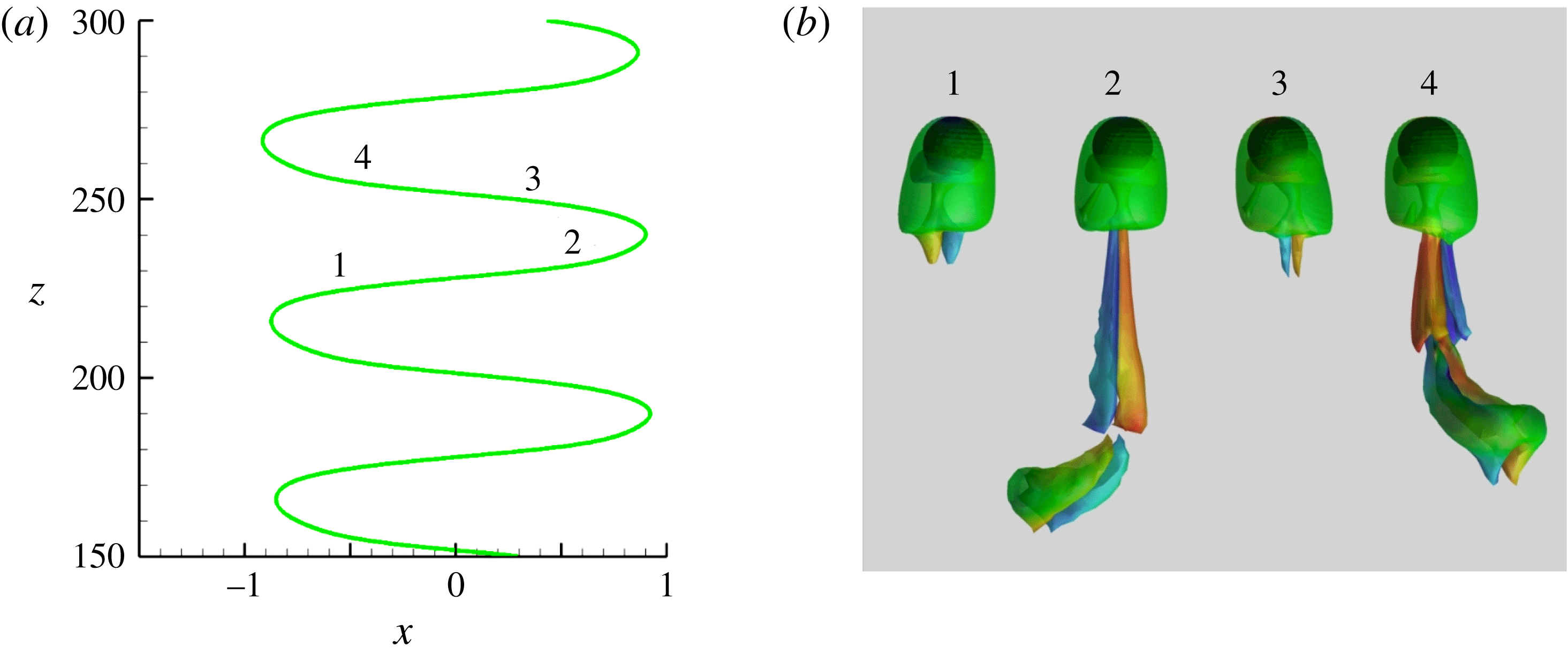
Figure 7. Characteristics of the ZZ regime for
 $\overline{\unicode[STIX]{x1D70C}}=0.5$
and
$\overline{\unicode[STIX]{x1D70C}}=0.5$
and
 $Ar=212.5$
. (a) Sphere trajectory; (b) wake evolution during
$Ar=212.5$
. (a) Sphere trajectory; (b) wake evolution during
 $3/4$
of a period visualized with the
$3/4$
of a period visualized with the
 $\unicode[STIX]{x1D706}_{2}$
criterion (
$\unicode[STIX]{x1D706}_{2}$
criterion (
 $-5.0\leqslant \unicode[STIX]{x1D714}_{z}\leqslant 5.0$
, see figure 4 for caption).
$-5.0\leqslant \unicode[STIX]{x1D714}_{z}\leqslant 5.0$
, see figure 4 for caption).
Figures 7 and 8, taken at the slightly larger Archimedes number
 $Ar=212.5$
, display a zoom of the typical sphere trajectory and the correspondence between path oscillations and wake dynamics in the ZZ and ZO regimes, respectively. As could be anticipated from figure 6, the sphere dynamics in the ZZ regime generally involves several harmonics of the fundamental frequency, so that the path is not a pure sinusoid; as shown by JDB, symmetry conditions imply that only odd harmonics are present. The simulations indicate that the dominant frequency, which governs the reversal of the horizontal velocity, is an increasing function of both
$Ar=212.5$
, display a zoom of the typical sphere trajectory and the correspondence between path oscillations and wake dynamics in the ZZ and ZO regimes, respectively. As could be anticipated from figure 6, the sphere dynamics in the ZZ regime generally involves several harmonics of the fundamental frequency, so that the path is not a pure sinusoid; as shown by JDB, symmetry conditions imply that only odd harmonics are present. The simulations indicate that the dominant frequency, which governs the reversal of the horizontal velocity, is an increasing function of both
 $Ar$
and
$Ar$
and
 $\overline{\unicode[STIX]{x1D70C}}$
, with
$\overline{\unicode[STIX]{x1D70C}}$
, with
 $St$
ranging from
$St$
ranging from
 $0.016$
to
$0.016$
to
 $0.036$
(
$0.036$
(
 $St\approx 0.02$
in the case displayed in figure 7). As shown in figure 7(b), two distinct shedding sequences are involved. That is, two pairs of counter-rotating vortices with opposite signs of the streamwise vorticity are successively shed in the wake during a zigzag half-period but one pair is much stronger than the other, keeping the path close to a sinusoid. The generation of the dominant pair starts just after the sphere has left one extremity of the zigzag (stages 1 and 3 in figure 7). This pair grows gradually until it forms a horseshoe vortex that detaches from the sphere approximately when it passes through the inflection point, i.e. midway between stages 1–2 or 3–4 (the remnants of this primary horseshoe vortex are still visible in the bottom part of stages 2 and 4 in figure 7(b)). The secondary pair, in which the streamwise vorticity within a given thread has changed sign compared to the primary pair, starts growing right after this shedding. It reaches its maximum magnitude approximately between the inflection point and the next extremity of the zigzag, i.e. in stages 2 and 4, and detaches from the sphere short before the latter reaches that extremity. A similar sequence was first observed experimentally by Horowitz & Williamson (Reference Horowitz and Williamson2010) with freely rising spheres and was referred to as the ‘4R’ shedding mode. It was also detected with nearly spheroidal rising bubbles in the recent computational study of Cano-Lozano et al. (Reference Cano-Lozano, Martínez-Bazán, Magnaudet and Tchoufag2016). In both cases, the body was found to follow a zigzagging path, so that this shedding mode appears to be intimately associated with this specific path geometry. However, for other sets of control parameters but still in the zigzagging regime, a ‘2R’ shedding mode with only one horseshoe vortex shed during each half-period of the path was also found in both studies. The mechanism that selects the ‘4R’ mode appears to be connected to the existence of oscillations in the rise velocity: when these oscillations (with frequency
$St\approx 0.02$
in the case displayed in figure 7). As shown in figure 7(b), two distinct shedding sequences are involved. That is, two pairs of counter-rotating vortices with opposite signs of the streamwise vorticity are successively shed in the wake during a zigzag half-period but one pair is much stronger than the other, keeping the path close to a sinusoid. The generation of the dominant pair starts just after the sphere has left one extremity of the zigzag (stages 1 and 3 in figure 7). This pair grows gradually until it forms a horseshoe vortex that detaches from the sphere approximately when it passes through the inflection point, i.e. midway between stages 1–2 or 3–4 (the remnants of this primary horseshoe vortex are still visible in the bottom part of stages 2 and 4 in figure 7(b)). The secondary pair, in which the streamwise vorticity within a given thread has changed sign compared to the primary pair, starts growing right after this shedding. It reaches its maximum magnitude approximately between the inflection point and the next extremity of the zigzag, i.e. in stages 2 and 4, and detaches from the sphere short before the latter reaches that extremity. A similar sequence was first observed experimentally by Horowitz & Williamson (Reference Horowitz and Williamson2010) with freely rising spheres and was referred to as the ‘4R’ shedding mode. It was also detected with nearly spheroidal rising bubbles in the recent computational study of Cano-Lozano et al. (Reference Cano-Lozano, Martínez-Bazán, Magnaudet and Tchoufag2016). In both cases, the body was found to follow a zigzagging path, so that this shedding mode appears to be intimately associated with this specific path geometry. However, for other sets of control parameters but still in the zigzagging regime, a ‘2R’ shedding mode with only one horseshoe vortex shed during each half-period of the path was also found in both studies. The mechanism that selects the ‘4R’ mode appears to be connected to the existence of oscillations in the rise velocity: when these oscillations (with frequency
 $2St$
, owing to obvious symmetry constraints) have a significant magnitude (typically 5 %), the ‘4R’ mode emerges, whereas the usual ‘2R’ mode is observed when they remain small (typically 1 % or less).
$2St$
, owing to obvious symmetry constraints) have a significant magnitude (typically 5 %), the ‘4R’ mode emerges, whereas the usual ‘2R’ mode is observed when they remain small (typically 1 % or less).
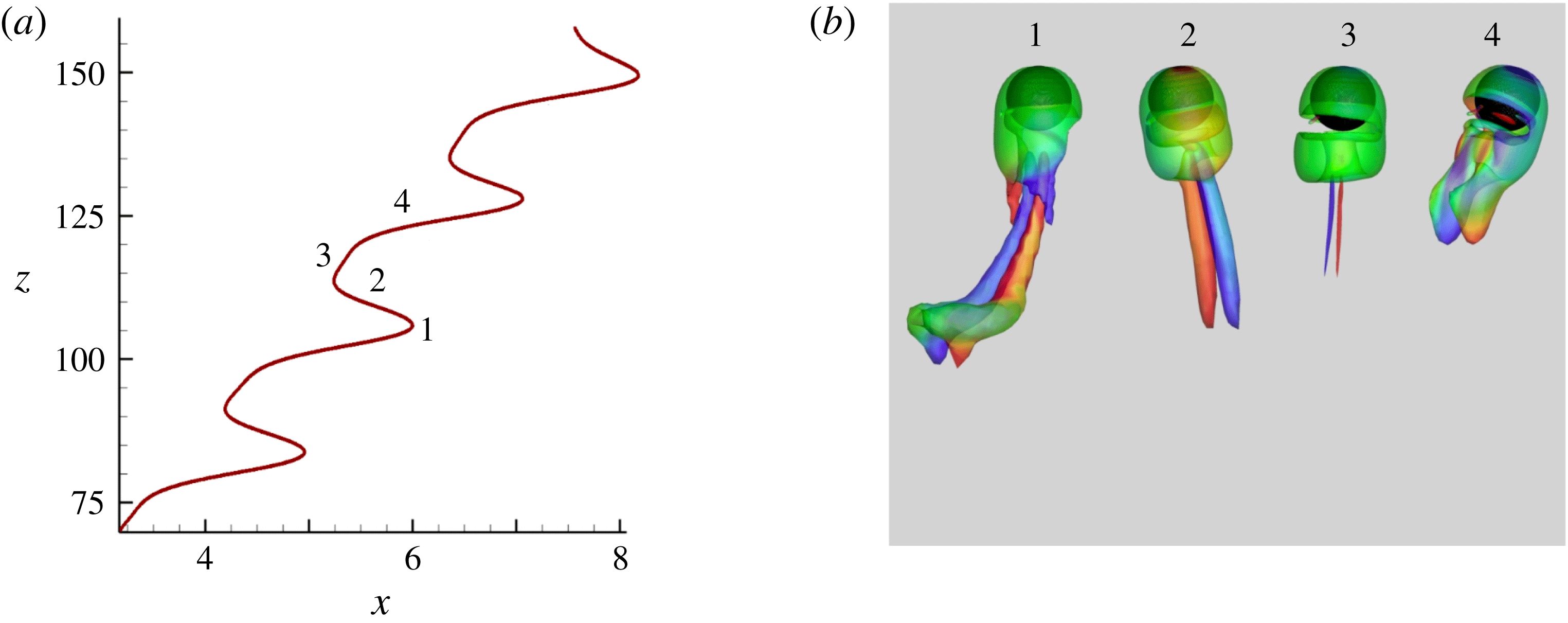
Figure 8. Characteristics of the ZO regime for
 $\overline{\unicode[STIX]{x1D70C}}=0.01$
and
$\overline{\unicode[STIX]{x1D70C}}=0.01$
and
 $Ar=212.5$
. (a) Sphere trajectory; (b) wake evolution during
$Ar=212.5$
. (a) Sphere trajectory; (b) wake evolution during
 $3/4$
of a period visualized with the
$3/4$
of a period visualized with the
 $\unicode[STIX]{x1D706}_{2}$
criterion (
$\unicode[STIX]{x1D706}_{2}$
criterion (
 $-4.34\leqslant \unicode[STIX]{x1D714}_{z}\leqslant 4.34$
, see figure 4 for caption).
$-4.34\leqslant \unicode[STIX]{x1D714}_{z}\leqslant 4.34$
, see figure 4 for caption).
Figure 8 displays the same information for the ZO path observed, still for
 $Ar=212.5$
, when the sphere-to-fluid density ratio is decreased to
$Ar=212.5$
, when the sphere-to-fluid density ratio is decreased to
 $\overline{\unicode[STIX]{x1D70C}}=0.01$
. The zigzags are now strongly asymmetric and the average path is inclined by approximately
$\overline{\unicode[STIX]{x1D70C}}=0.01$
. The zigzags are now strongly asymmetric and the average path is inclined by approximately
 $3.6^{\circ }$
with respect to the vertical. The Strouhal number is approximately
$3.6^{\circ }$
with respect to the vertical. The Strouhal number is approximately
 $0.046$
, which is significantly larger than in the ZZ regime. Again, the evolution of the corresponding wake structure reveals that four pairs of counter-rotating vortices are shed downstream during a period. However, in contrast to ZZ paths, the sign of the streamwise vorticity changes every time a new pair appears. Hence, considering the thread located on a given half-space with respect to the plane of rise, the successive stages 1–4 in figure 7 correspond to, say, a
$0.046$
, which is significantly larger than in the ZZ regime. Again, the evolution of the corresponding wake structure reveals that four pairs of counter-rotating vortices are shed downstream during a period. However, in contrast to ZZ paths, the sign of the streamwise vorticity changes every time a new pair appears. Hence, considering the thread located on a given half-space with respect to the plane of rise, the successive stages 1–4 in figure 7 correspond to, say, a
 $+--+$
sequence, whereas those in figure 8 correspond to a
$+--+$
sequence, whereas those in figure 8 correspond to a
 $+-+-$
one. Moreover, one pair (instead of two in the ZZ regime) is much stronger than the other three (respectively two) and is responsible for the lateral drift (this pair is the one that starts growing when the horizontal velocity reverses almost symmetrically, i.e. in stage 1 of figure 8).
$+-+-$
one. Moreover, one pair (instead of two in the ZZ regime) is much stronger than the other three (respectively two) and is responsible for the lateral drift (this pair is the one that starts growing when the horizontal velocity reverses almost symmetrically, i.e. in stage 1 of figure 8).
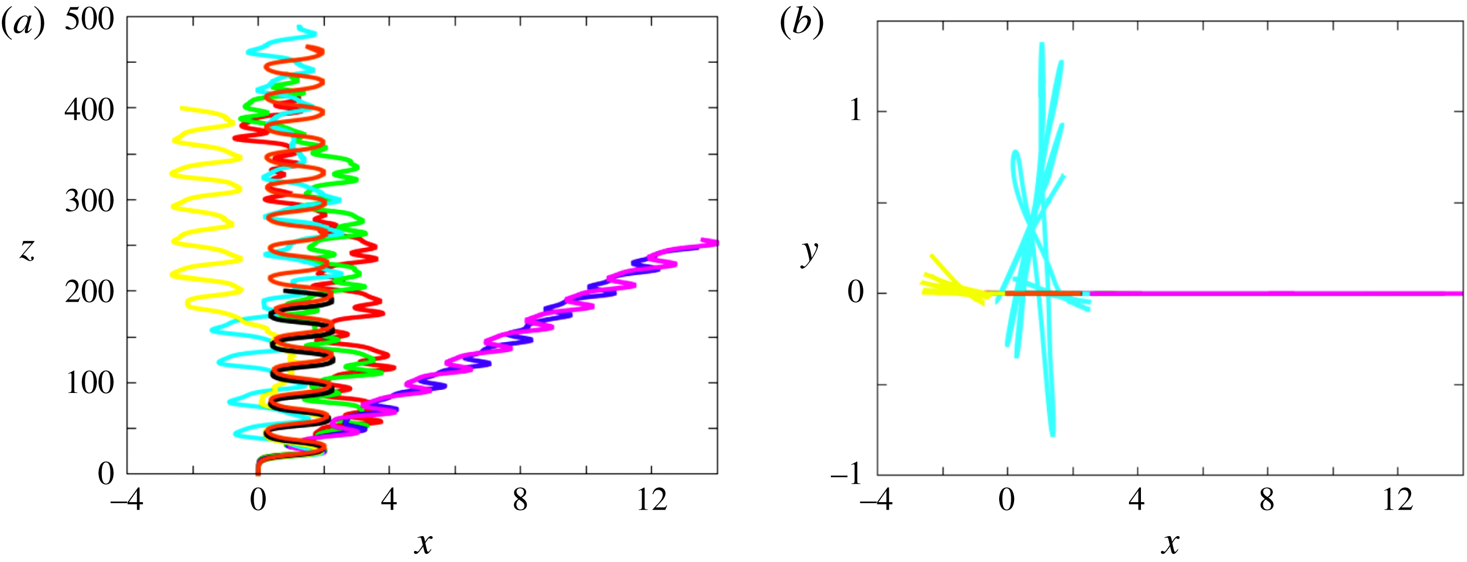
Figure 9. Paths for various solid-to-fluid density ratios at
 $Ar=237.5$
; (a) projection onto the vertical
$Ar=237.5$
; (a) projection onto the vertical
 $(x,z)$
plane, (b) projection onto the horizontal plane. Same colour code as in figure 6.
$(x,z)$
plane, (b) projection onto the horizontal plane. Same colour code as in figure 6.

Figure 10. Velocity diagrams built on the vertical
 $(V_{v})$
and horizontal
$(V_{v})$
and horizontal
 $(V_{h})$
sphere velocities (both normalized with
$(V_{h})$
sphere velocities (both normalized with
 $V_{g}$
), obtained for spheres with
$V_{g}$
), obtained for spheres with
 $\overline{\unicode[STIX]{x1D70C}}=0.01$
in the various regimes encountered in the range
$\overline{\unicode[STIX]{x1D70C}}=0.01$
in the various regimes encountered in the range
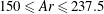 $150\leqslant Ar\leqslant 237.5$
. Diagrams corresponding to the three successive intermittent (IT) regimes observed for
$150\leqslant Ar\leqslant 237.5$
. Diagrams corresponding to the three successive intermittent (IT) regimes observed for
 $Ar=172$
(a),
$Ar=172$
(a),
 $187.5$
(b) and
$187.5$
(b) and
 $237.5$
(c) are compared with those found in the successive stationary and periodic regimes, namely SV (
$237.5$
(c) are compared with those found in the successive stationary and periodic regimes, namely SV (
 $Ar=150$
), SO (
$Ar=150$
), SO (
 $Ar=162.5$
), PO (
$Ar=162.5$
), PO (
 $Ar=166$
), ZZ (
$Ar=166$
), ZZ (
 $Ar=178$
) and ZO (
$Ar=178$
) and ZO (
 $Ar=200$
). The colour scale refers to that used in the state diagrams of figures 2 and 13; a horizontal flip has been applied to the ZO curve to make the figure clearer.
$Ar=200$
). The colour scale refers to that used in the state diagrams of figures 2 and 13; a horizontal flip has been applied to the ZO curve to make the figure clearer.
We observe the ZO regime typically in the range
 $200\leqslant Ar\leqslant 250$
for density ratios that may be up to
$200\leqslant Ar\leqslant 250$
for density ratios that may be up to
 $0.175$
. The corresponding ‘island’ in the
$0.175$
. The corresponding ‘island’ in the
 $(Ar,\overline{\unicode[STIX]{x1D70C}})$
diagram (see figure 13 below) has a limited area and looks like a thin stripe, the right edge of which makes a positive angle with respect to the
$(Ar,\overline{\unicode[STIX]{x1D70C}})$
diagram (see figure 13 below) has a limited area and looks like a thin stripe, the right edge of which makes a positive angle with respect to the
 $Ar$
-axis. Indeed, increasing
$Ar$
-axis. Indeed, increasing
 $Ar$
within the ZO regime, the path of the lightest sphere (
$Ar$
within the ZO regime, the path of the lightest sphere (
 $\overline{\unicode[STIX]{x1D70C}}=0.001$
) starts to exhibit some intermittency for
$\overline{\unicode[STIX]{x1D70C}}=0.001$
) starts to exhibit some intermittency for
 $Ar=212.5$
after the sphere has risen a vertical distance of
$Ar=212.5$
after the sphere has risen a vertical distance of
 $O(150d)$
. Other very light spheres switch similarly from a ZO path to an intermittent path at a critical
$O(150d)$
. Other very light spheres switch similarly from a ZO path to an intermittent path at a critical
 $Ar$
increasing with
$Ar$
increasing with
 $\overline{\unicode[STIX]{x1D70C}}$
. Thus the lightest sphere still exhibiting a periodic ZO path when
$\overline{\unicode[STIX]{x1D70C}}$
. Thus the lightest sphere still exhibiting a periodic ZO path when
 $Ar=237.5$
corresponds to
$Ar=237.5$
corresponds to
 $\overline{\unicode[STIX]{x1D70C}}=0.05$
. At the same time, the maximum
$\overline{\unicode[STIX]{x1D70C}}=0.05$
. At the same time, the maximum
 $\overline{\unicode[STIX]{x1D70C}}$
at which a ZO path is observed also increases with
$\overline{\unicode[STIX]{x1D70C}}$
at which a ZO path is observed also increases with
 $Ar$
, from
$Ar$
, from
 $0.05$
for
$0.05$
for
 $Ar=200$
to
$Ar=200$
to
 $0.175$
for
$0.175$
for
 $Ar=250$
. Consequently, as figure 9(a) shows, only spheres with
$Ar=250$
. Consequently, as figure 9(a) shows, only spheres with
 $\overline{\unicode[STIX]{x1D70C}}=0.05$
and
$\overline{\unicode[STIX]{x1D70C}}=0.05$
and
 $\overline{\unicode[STIX]{x1D70C}}=0.1$
still exhibit a periodic ZO path at
$\overline{\unicode[STIX]{x1D70C}}=0.1$
still exhibit a periodic ZO path at
 $Ar=237.5$
. Figure 9(b) indicates that these paths are still planar. The same conclusion holds for the intermittent paths observed with the lightest two spheres, as well as for the periodic ZZ paths of the two heaviest ones. In contrast, the two intermediate spheres corresponding to
$Ar=237.5$
. Figure 9(b) indicates that these paths are still planar. The same conclusion holds for the intermittent paths observed with the lightest two spheres, as well as for the periodic ZZ paths of the two heaviest ones. In contrast, the two intermediate spheres corresponding to
 $\overline{\unicode[STIX]{x1D70C}}=0.25$
and
$\overline{\unicode[STIX]{x1D70C}}=0.25$
and
 $\overline{\unicode[STIX]{x1D70C}}=0.5$
develop a strikingly different behaviour. They both follow an intermittent large-amplitude zigzagging path. However, every time a ‘hesitation’ of the zigzag happens, a new symmetry plane is selected for the next, almost periodic, zigzagging sequence. As a result, these paths lose their planarity after the first defect, i.e. for
$\overline{\unicode[STIX]{x1D70C}}=0.5$
develop a strikingly different behaviour. They both follow an intermittent large-amplitude zigzagging path. However, every time a ‘hesitation’ of the zigzag happens, a new symmetry plane is selected for the next, almost periodic, zigzagging sequence. As a result, these paths lose their planarity after the first defect, i.e. for
 $z\gtrsim 100d$
and
$z\gtrsim 100d$
and
 $150d$
, respectively. At lower values of
$150d$
, respectively. At lower values of
 $Ar$
, the maximum out-of-plane path deviations we measured were always less than
$Ar$
, the maximum out-of-plane path deviations we measured were always less than
 $10^{-2}d$
, and most frequently less than
$10^{-2}d$
, and most frequently less than
 $10^{-5}d$
. Here in contrast the ratio of the maximum horizontal excursions in two perpendicular directions is of
$10^{-5}d$
. Here in contrast the ratio of the maximum horizontal excursions in two perpendicular directions is of
 $O(1)$
. Hence
$O(1)$
. Hence
 $Ar=237.5$
marks the threshold beyond which intermittent paths start to exhibit a clear three-dimensionality. Interestingly, since
$Ar=237.5$
marks the threshold beyond which intermittent paths start to exhibit a clear three-dimensionality. Interestingly, since
 $V_{m}\approx 1.45V_{g}$
at this value of
$V_{m}\approx 1.45V_{g}$
at this value of
 $Ar$
, the average Reynolds number
$Ar$
, the average Reynolds number
 $Re_{m}$
is close to
$Re_{m}$
is close to
 $350$
, which is approximately the critical value beyond which three-dimensionality is known to exist in the wake of a sphere held fixed in a uniform stream (Mittal Reference Mittal1999).
$350$
, which is approximately the critical value beyond which three-dimensionality is known to exist in the wake of a sphere held fixed in a uniform stream (Mittal Reference Mittal1999).
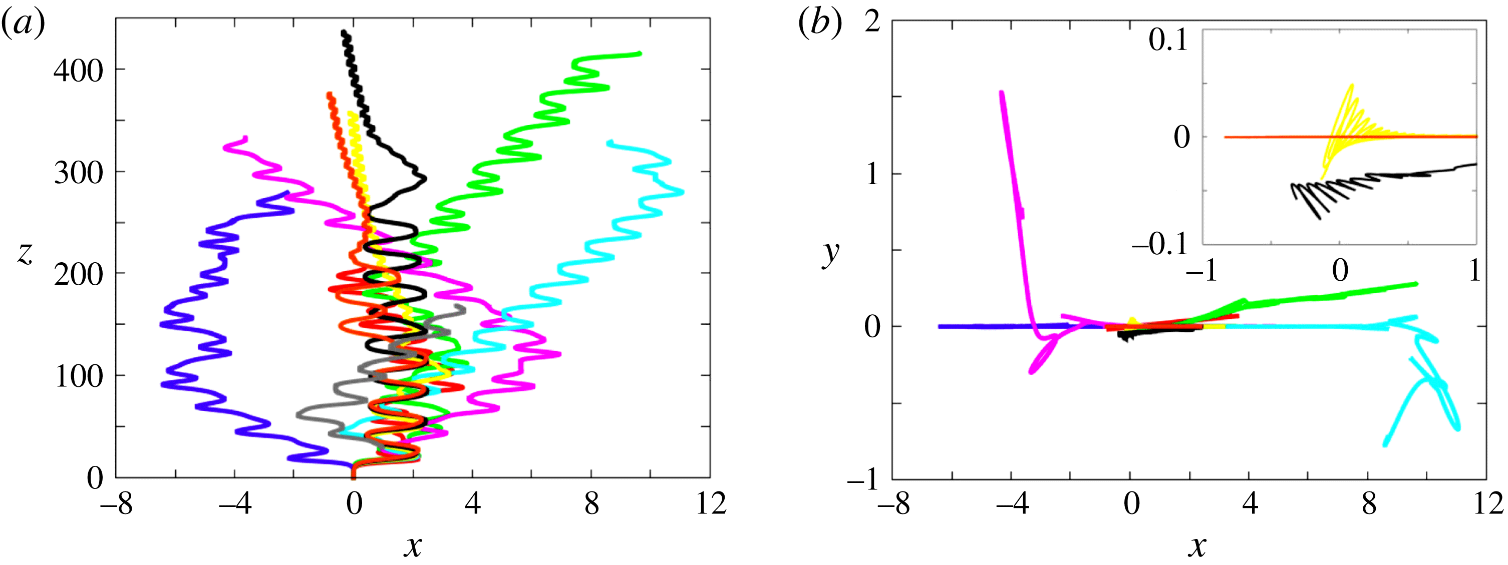
Figure 11. Paths for various solid-to-fluid density ratios at
 $Ar=275$
; (a) projection onto the vertical
$Ar=275$
; (a) projection onto the vertical
 $(x,z)$
plane, (b) projection onto the horizontal plane (with a zoom for
$(x,z)$
plane, (b) projection onto the horizontal plane (with a zoom for
 $\overline{\unicode[STIX]{x1D70C}}=0.5,0.75$
and
$\overline{\unicode[STIX]{x1D70C}}=0.5,0.75$
and
 $0.99$
). Same colour code as in figure 6.
$0.99$
). Same colour code as in figure 6.
The chaotic or periodic nature of the various regimes encountered with very light spheres (
 $\overline{\unicode[STIX]{x1D70C}}=0.01$
) up to
$\overline{\unicode[STIX]{x1D70C}}=0.01$
) up to
 $Ar=237.5$
is made apparent in figure 10, using phase portraits built on the two components of the body velocity (the transients corresponding to the initial vertical rise were removed so as to focus on the ulterior evolution). Increasing the Archimedes number from
$Ar=237.5$
is made apparent in figure 10, using phase portraits built on the two components of the body velocity (the transients corresponding to the initial vertical rise were removed so as to focus on the ulterior evolution). Increasing the Archimedes number from
 $Ar=150$
, the system successively stands (see figures 2 and 13) in the SV, SO, PO, IT, ZZ, IT, ZO and IT regimes (in our nomenclature, the IT label gathers all intermittent regimes, even though they sometimes occupy separate areas in the
$Ar=150$
, the system successively stands (see figures 2 and 13) in the SV, SO, PO, IT, ZZ, IT, ZO and IT regimes (in our nomenclature, the IT label gathers all intermittent regimes, even though they sometimes occupy separate areas in the
 $(Ar,\,\overline{\unicode[STIX]{x1D70C}})$
plane). Curves associated with the three successive intermittent regimes tend to fill densely a region of the
$(Ar,\,\overline{\unicode[STIX]{x1D70C}})$
plane). Curves associated with the three successive intermittent regimes tend to fill densely a region of the
 $(V_{v},V_{h})$
plane, demonstrating the chaotic nature of the corresponding paths. The rate at which this filling operates clearly increases with
$(V_{v},V_{h})$
plane, demonstrating the chaotic nature of the corresponding paths. The rate at which this filling operates clearly increases with
 $Ar$
(the three graphs were obtained by considering the velocity evolution over a similar height), highlighting the fact that the system becomes more and more chaotic as
$Ar$
(the three graphs were obtained by considering the velocity evolution over a similar height), highlighting the fact that the system becomes more and more chaotic as
 $Ar$
increases. The phase portrait corresponding to the ZZ regime displays a slight asymmetry in the region corresponding to the maxima of the lateral sphere excursion (
$Ar$
increases. The phase portrait corresponding to the ZZ regime displays a slight asymmetry in the region corresponding to the maxima of the lateral sphere excursion (
 $V_{h}\approx 0$
), underlining the influence of higher harmonics on the sphere kinematics. In the ZO regime, a long transient precedes the fully periodic evolution. Then, unlike the Lissajous-type curve characterizing the ZZ regime, the phase portrait consists of a single, highly asymmetric, loop. This is because the vertical velocity takes two different values at the two locations where the horizontal velocity changes sign, which is not unlikely given the strong asymmetry of the path around points 1 and 3 in figure 8. Note also the sharp bump associated with the maximum of
$V_{h}\approx 0$
), underlining the influence of higher harmonics on the sphere kinematics. In the ZO regime, a long transient precedes the fully periodic evolution. Then, unlike the Lissajous-type curve characterizing the ZZ regime, the phase portrait consists of a single, highly asymmetric, loop. This is because the vertical velocity takes two different values at the two locations where the horizontal velocity changes sign, which is not unlikely given the strong asymmetry of the path around points 1 and 3 in figure 8. Note also the sharp bump associated with the maximum of
 $V_{v}$
, which corresponds to the region in between points 3 and 4 in figure 8 where the path remains almost vertical during a significant time lapse.
$V_{v}$
, which corresponds to the region in between points 3 and 4 in figure 8 where the path remains almost vertical during a significant time lapse.
Figure 12. Characteristics of the ZZ
 $_{2}$
regime for
$_{2}$
regime for
 $\overline{\unicode[STIX]{x1D70C}}=0.5$
and
$\overline{\unicode[STIX]{x1D70C}}=0.5$
and
 $Ar=300$
. (a) Sphere trajectory; (b) wake evolution during
$Ar=300$
. (a) Sphere trajectory; (b) wake evolution during
 $3/4$
of a period visualized with the
$3/4$
of a period visualized with the
 $\unicode[STIX]{x1D706}_{2}$
criterion (
$\unicode[STIX]{x1D706}_{2}$
criterion (
 $-4.73\leqslant \unicode[STIX]{x1D714}_{z}\leqslant 4.73$
, see figure 4 for caption).
$-4.73\leqslant \unicode[STIX]{x1D714}_{z}\leqslant 4.73$
, see figure 4 for caption).
In the range
 $250\lesssim Ar\lesssim 300$
, a new regime is observed for large enough solid-to-fluid density ratios, mostly
$250\lesssim Ar\lesssim 300$
, a new regime is observed for large enough solid-to-fluid density ratios, mostly
 $\overline{\unicode[STIX]{x1D70C}}\gtrsim 0.5$
. Figure 11 provides typical examples of that regime by displaying the various paths for
$\overline{\unicode[STIX]{x1D70C}}\gtrsim 0.5$
. Figure 11 provides typical examples of that regime by displaying the various paths for
 $Ar=275$
. All spheres with
$Ar=275$
. All spheres with
 $\overline{\unicode[STIX]{x1D70C}}<0.5$
follow intermittent paths, some of them being fully three-dimensional (see below for the definition of the corresponding IT regime). Nevertheless, in the range
$\overline{\unicode[STIX]{x1D70C}}<0.5$
follow intermittent paths, some of them being fully three-dimensional (see below for the definition of the corresponding IT regime). Nevertheless, in the range
 $0.05\leqslant \overline{\unicode[STIX]{x1D70C}}\leqslant 0.25$
, long sequences reminiscent of the ZO regime are still noticed. As figure 11(b) shows, several of the corresponding trajectories are strongly three-dimensional but some others remain planar. The three heaviest spheres, corresponding to
$0.05\leqslant \overline{\unicode[STIX]{x1D70C}}\leqslant 0.25$
, long sequences reminiscent of the ZO regime are still noticed. As figure 11(b) shows, several of the corresponding trajectories are strongly three-dimensional but some others remain planar. The three heaviest spheres, corresponding to
 $\overline{\unicode[STIX]{x1D70C}}\geqslant 0.5$
, start by following a well-defined large-amplitude planar zigzagging trajectory. However, this path becomes unstable at some point and the zigzags disappear. After a transitional stage, a new style of path emerges in the form of another zigzagging motion with characteristics distinctly different from those of the ZZ regime. This new regime, which we refer to as ZZ
$\overline{\unicode[STIX]{x1D70C}}\geqslant 0.5$
, start by following a well-defined large-amplitude planar zigzagging trajectory. However, this path becomes unstable at some point and the zigzags disappear. After a transitional stage, a new style of path emerges in the form of another zigzagging motion with characteristics distinctly different from those of the ZZ regime. This new regime, which we refer to as ZZ
 $_{2}$
, is characterized by small-amplitude high-frequency lateral sphere displacements: in the example of figure 11, the crest-to-crest amplitude is typically approximately 20 % of the sphere diameter and the Strouhal number is close to
$_{2}$
, is characterized by small-amplitude high-frequency lateral sphere displacements: in the example of figure 11, the crest-to-crest amplitude is typically approximately 20 % of the sphere diameter and the Strouhal number is close to
 $0.1$
. For other
$0.1$
. For other
 $(Ar,\,\overline{\unicode[STIX]{x1D70C}})$
sets, the Strouhal number stays in the range 0.10–0.11 and the crest-to-crest amplitude is always less than
$(Ar,\,\overline{\unicode[STIX]{x1D70C}})$
sets, the Strouhal number stays in the range 0.10–0.11 and the crest-to-crest amplitude is always less than
 $0.3d$
. Hence, compared to the ZZ regime, the amplitude of the zigzags is typically one order of magnitude smaller, whereas their frequency is three to five times larger. Several additional features of the ZZ
$0.3d$
. Hence, compared to the ZZ regime, the amplitude of the zigzags is typically one order of magnitude smaller, whereas their frequency is three to five times larger. Several additional features of the ZZ
 $_{2}$
regime are made apparent in figure 11. First, unlike the ZZ and ZO paths, the ZZ
$_{2}$
regime are made apparent in figure 11. First, unlike the ZZ and ZO paths, the ZZ
 $_{2}$
path is found to emerge after a (very) long transient (up to
$_{2}$
path is found to emerge after a (very) long transient (up to
 ${\approx}330d$
for
${\approx}330d$
for
 $\overline{\unicode[STIX]{x1D70C}}=0.75$
). Next, it may be noticed that in this regime the sphere drifts slowly but consistently throughout its ascent, which implies that its wake delivers a non-zero average lift force. Last, as the inset in figure 11(b) reveals, ZZ
$\overline{\unicode[STIX]{x1D70C}}=0.75$
). Next, it may be noticed that in this regime the sphere drifts slowly but consistently throughout its ascent, which implies that its wake delivers a non-zero average lift force. Last, as the inset in figure 11(b) reveals, ZZ
 $_{2}$
paths are generally non-planar because the plane within which the zigzags take place slowly rotates.
$_{2}$
paths are generally non-planar because the plane within which the zigzags take place slowly rotates.
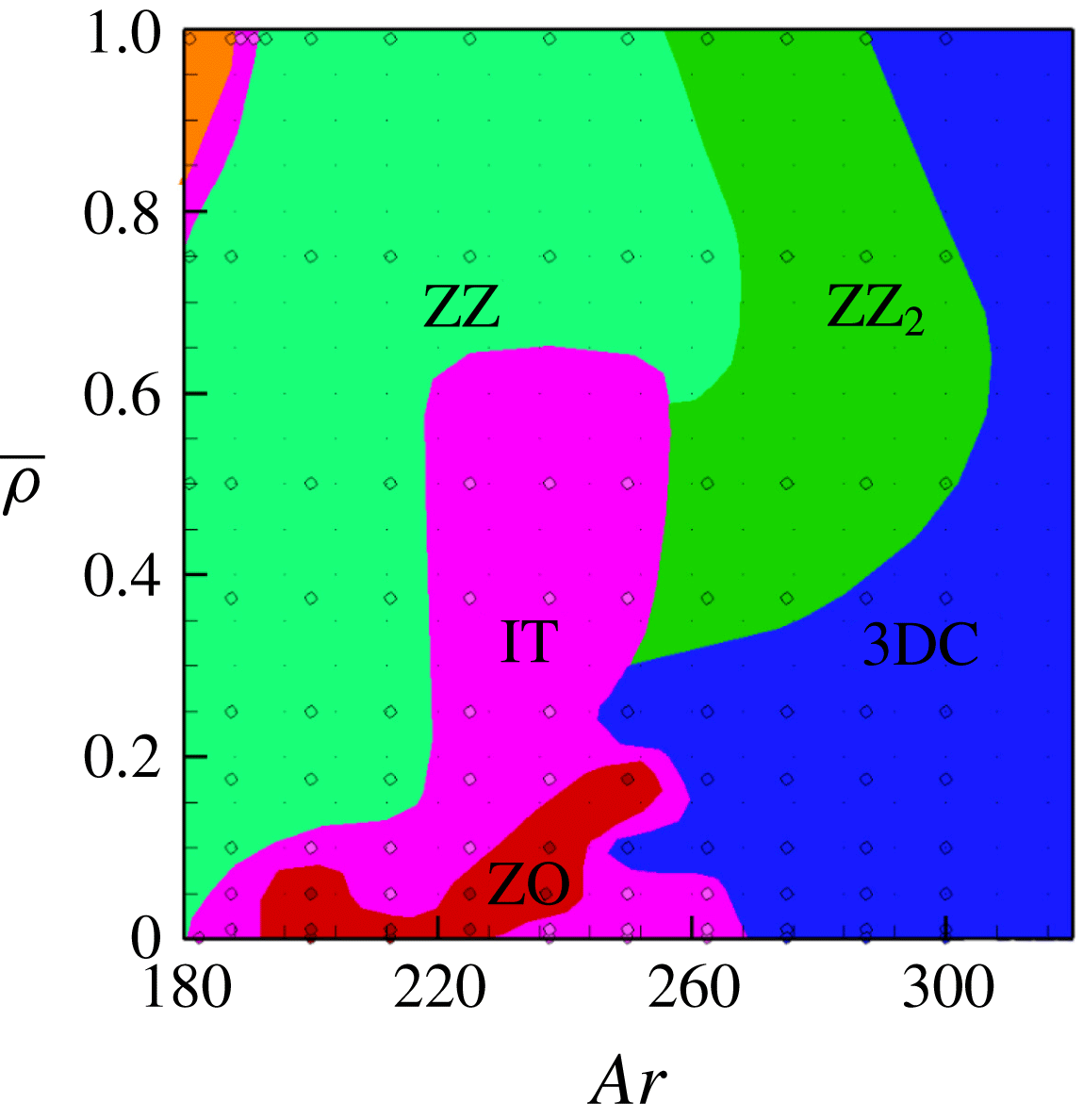
Figure 13. State diagram of rise regimes in the intermediate range
 $180\leqslant Ar\leqslant 320$
. Dark orange: periodic oblique (PO); purple: intermittent (IT); green: large-amplitude zigzagging (ZZ); red: zigzagging oblique (ZO); dark green: small-amplitude zigzagging (ZZ
$180\leqslant Ar\leqslant 320$
. Dark orange: periodic oblique (PO); purple: intermittent (IT); green: large-amplitude zigzagging (ZZ); red: zigzagging oblique (ZO); dark green: small-amplitude zigzagging (ZZ
 $_{2}$
); blue: three-dimensional chaotic (3DC).
$_{2}$
); blue: three-dimensional chaotic (3DC).
Figure 12 shows the correspondence between path oscillations and wake dynamics in the case
 $\overline{\unicode[STIX]{x1D70C}}=0.5,Ar=300$
; for this set of parameters, the amplitude of the out-of-plane horizontal motions is less than 4 % of that of in-plane excursions so that the path is nearly two-dimensional. The streamwise vorticity in a given trailing vortex is seen to keep the same sign in stages 1–4 and 2–3, respectively. Hence this quantity only changes sign every time the sphere crosses the inflection point of the zigzag, so that only two vortex pairs are released downstream during a ZZ
$\overline{\unicode[STIX]{x1D70C}}=0.5,Ar=300$
; for this set of parameters, the amplitude of the out-of-plane horizontal motions is less than 4 % of that of in-plane excursions so that the path is nearly two-dimensional. The streamwise vorticity in a given trailing vortex is seen to keep the same sign in stages 1–4 and 2–3, respectively. Hence this quantity only changes sign every time the sphere crosses the inflection point of the zigzag, so that only two vortex pairs are released downstream during a ZZ
 $_{2}$
period, instead of four in the ZZ regime. It must be noticed that ZD also observed a rise/fall regime characterized by small-amplitude high-frequency oscillations with
$_{2}$
period, instead of four in the ZZ regime. It must be noticed that ZD also observed a rise/fall regime characterized by small-amplitude high-frequency oscillations with
 $St\approx 0.1$
for
$St\approx 0.1$
for
 $250\lesssim Ar\lesssim 300$
and
$250\lesssim Ar\lesssim 300$
and
 $0.5\lesssim \overline{\unicode[STIX]{x1D70C}}\lesssim 2.0$
. Hence, for rising spheres, there is a perfect match between the domains where regimes involving such fast oscillations are observed in both studies. However, ZD found the corresponding paths to be strictly planar and vertical on average, which led them to term this regime ‘vertical oscillating’. Hence, here again, some important structural characteristics of the zigzagging regime observed in the present study differ from those reported by ZD.
$0.5\lesssim \overline{\unicode[STIX]{x1D70C}}\lesssim 2.0$
. Hence, for rising spheres, there is a perfect match between the domains where regimes involving such fast oscillations are observed in both studies. However, ZD found the corresponding paths to be strictly planar and vertical on average, which led them to term this regime ‘vertical oscillating’. Hence, here again, some important structural characteristics of the zigzagging regime observed in the present study differ from those reported by ZD.
Figure 13 summarizes the succession of regimes encountered in the range
 $180\leqslant Ar\leqslant 300$
. It underlines the particularly strong influence of the sphere-to-fluid density ratio on the style of path in that range. The extent of the planar large-amplitude ZZ regime is quite remarkable. In particular, it is found to dominate the scene for spheres with
$180\leqslant Ar\leqslant 300$
. It underlines the particularly strong influence of the sphere-to-fluid density ratio on the style of path in that range. The extent of the planar large-amplitude ZZ regime is quite remarkable. In particular, it is found to dominate the scene for spheres with
 $\overline{\unicode[STIX]{x1D70C}}\gtrsim 0.1$
throughout the range
$\overline{\unicode[STIX]{x1D70C}}\gtrsim 0.1$
throughout the range
 $195\lesssim Ar\lesssim 220$
. This clearly differs from the findings of ZD who did not detect any large-amplitude zigzag for sphere-to-fluid density ratios larger than
$195\lesssim Ar\lesssim 220$
. This clearly differs from the findings of ZD who did not detect any large-amplitude zigzag for sphere-to-fluid density ratios larger than
 $0.5$
, nor for
$0.5$
, nor for
 $Ar>200$
. Up to
$Ar>200$
. Up to
 $Ar\approx 260$
, most situations for very light spheres, say
$Ar\approx 260$
, most situations for very light spheres, say
 $\overline{\unicode[STIX]{x1D70C}}\lesssim 0.1$
, correspond to intermittent regimes; note also the significant tongue of IT regimes in the range
$\overline{\unicode[STIX]{x1D70C}}\lesssim 0.1$
, correspond to intermittent regimes; note also the significant tongue of IT regimes in the range
 $220\lesssim Ar\lesssim 250$
which separates the ZZ and ZZ
$220\lesssim Ar\lesssim 250$
which separates the ZZ and ZZ
 $_{2}$
domains up to
$_{2}$
domains up to
 $\overline{\unicode[STIX]{x1D70C}}\approx 0.6$
. In all cases, these intermittent regimes are associated with planar paths below
$\overline{\unicode[STIX]{x1D70C}}\approx 0.6$
. In all cases, these intermittent regimes are associated with planar paths below
 $Ar\approx 235$
and with three-dimensional paths beyond that limit. Nevertheless, we do not classify the latter as fully three-dimensional chaotic (3DC), although both are of the same nature from a dynamical system viewpoint, because the observed three-dimensional intermittent paths still essentially exhibit the ZZ style, with only one or two defects throughout the entire path (see figure 9). This trend stops beyond a certain
$Ar\approx 235$
and with three-dimensional paths beyond that limit. Nevertheless, we do not classify the latter as fully three-dimensional chaotic (3DC), although both are of the same nature from a dynamical system viewpoint, because the observed three-dimensional intermittent paths still essentially exhibit the ZZ style, with only one or two defects throughout the entire path (see figure 9). This trend stops beyond a certain
 $Ar$
, and this is where we located the qualitative IT/3DC border in figure 13. We did the same with the ‘almost ZO’ intermittent paths found for
$Ar$
, and this is where we located the qualitative IT/3DC border in figure 13. We did the same with the ‘almost ZO’ intermittent paths found for
 $\overline{\unicode[STIX]{x1D70C}}\lesssim 0.175$
beyond the ZO regime.
$\overline{\unicode[STIX]{x1D70C}}\lesssim 0.175$
beyond the ZO regime.
Figure 14. Two three-dimensional paths in the 3DC regime at
 $Ar=350$
. (a)
$Ar=350$
. (a)
 $\overline{\unicode[STIX]{x1D70C}}=0.99$
, (b)
$\overline{\unicode[STIX]{x1D70C}}=0.99$
, (b)
 $\overline{\unicode[STIX]{x1D70C}}=0.05$
. The horizontal projection of the path is seen in the plane
$\overline{\unicode[STIX]{x1D70C}}=0.05$
. The horizontal projection of the path is seen in the plane
 $z=0$
.
$z=0$
.
3.4 Beyond
$Ar=300$

The ZZ
 $_{2}$
regime ends in the range
$_{2}$
regime ends in the range
 $260\lesssim Ar\lesssim 300$
, depending on
$260\lesssim Ar\lesssim 300$
, depending on
 $\overline{\unicode[STIX]{x1D70C}}$
. It is succeeded by the regime we refer to as 3DC, characterized by chaotic, fully three-dimensional paths in which only few traces of the previous periodic regime subsist. For
$\overline{\unicode[STIX]{x1D70C}}$
. It is succeeded by the regime we refer to as 3DC, characterized by chaotic, fully three-dimensional paths in which only few traces of the previous periodic regime subsist. For
 $\overline{\unicode[STIX]{x1D70C}}\lesssim 0.3$
, the same happens beyond the three-dimensional intermittent regime defined above.
$\overline{\unicode[STIX]{x1D70C}}\lesssim 0.3$
, the same happens beyond the three-dimensional intermittent regime defined above.
Figure 14 displays two trajectories characteristic of the 3DC regime at
 $Ar=350$
, for
$Ar=350$
, for
 $\overline{\unicode[STIX]{x1D70C}}=0.99$
and
$\overline{\unicode[STIX]{x1D70C}}=0.99$
and
 $\overline{\unicode[STIX]{x1D70C}}=0.05$
, respectively. The total lateral excursion of the sphere throughout its ascent is approximately
$\overline{\unicode[STIX]{x1D70C}}=0.05$
, respectively. The total lateral excursion of the sphere throughout its ascent is approximately
 $8d$
and
$8d$
and
 $5d$
, respectively. This is typical of what we observed in that regime, although significantly smaller values (
$5d$
, respectively. This is typical of what we observed in that regime, although significantly smaller values (
 ${\approx}2d$
) were noticed in several cases. No clear trend regarding variations of this amplitude as a function of
${\approx}2d$
) were noticed in several cases. No clear trend regarding variations of this amplitude as a function of
 $\overline{\unicode[STIX]{x1D70C}}$
and
$\overline{\unicode[STIX]{x1D70C}}$
and
 $Ar$
emerged from the simulations throughout the explored range corresponding to the 3DC regime. In contrast, figure 14 reveals a striking difference between the dynamics of ‘light’ and ‘heavy’ spheres, the former repeatedly experiencing large lateral deviations over short periods of time. In other words, the horizontal fluctuations of the instantaneous sphere velocity are found to be much larger for
$Ar$
emerged from the simulations throughout the explored range corresponding to the 3DC regime. In contrast, figure 14 reveals a striking difference between the dynamics of ‘light’ and ‘heavy’ spheres, the former repeatedly experiencing large lateral deviations over short periods of time. In other words, the horizontal fluctuations of the instantaneous sphere velocity are found to be much larger for
 $\overline{\unicode[STIX]{x1D70C}}=0.05$
than for
$\overline{\unicode[STIX]{x1D70C}}=0.05$
than for
 $\overline{\unicode[STIX]{x1D70C}}=0.99$
. This trend subsists until the upper limit of our simulations, i.e.
$\overline{\unicode[STIX]{x1D70C}}=0.99$
. This trend subsists until the upper limit of our simulations, i.e.
 $Ar=700$
. It is in line with the findings reported by ZD who, for
$Ar=700$
. It is in line with the findings reported by ZD who, for
 $Ar=350$
, noticed root-mean-square horizontal velocity fluctuations approximately twice as large for
$Ar=350$
, noticed root-mean-square horizontal velocity fluctuations approximately twice as large for
 $\overline{\unicode[STIX]{x1D70C}}\approx 0$
than for
$\overline{\unicode[STIX]{x1D70C}}\approx 0$
than for
 $\overline{\unicode[STIX]{x1D70C}}\lesssim 1$
. This increase of horizontal velocity fluctuations for light spheres has a direct consequence on the rise velocity: since a larger part of the potential energy available in the system is used to ‘feed’ horizontal motions, less energy is injected in the vertical direction, resulting in a reduction of the average rise velocity. This is why, in the example of figure 14, the rise velocity of the lighter sphere is smaller by approximately 6 % than that of the ‘heavy’ one.
$\overline{\unicode[STIX]{x1D70C}}\lesssim 1$
. This increase of horizontal velocity fluctuations for light spheres has a direct consequence on the rise velocity: since a larger part of the potential energy available in the system is used to ‘feed’ horizontal motions, less energy is injected in the vertical direction, resulting in a reduction of the average rise velocity. This is why, in the example of figure 14, the rise velocity of the lighter sphere is smaller by approximately 6 % than that of the ‘heavy’ one.
Figure 15. Paths for various solid-to-fluid density ratios at
 $Ar=400$
; (a) projection onto the vertical
$Ar=400$
; (a) projection onto the vertical
 $(x,z)$
plane, (b) projection onto the horizontal plane. Same colour code as in figure 6.
$(x,z)$
plane, (b) projection onto the horizontal plane. Same colour code as in figure 6.
The specificity of very light spheres takes a spectacular turn for
 $Ar\geqslant 400$
, as figure 15 shows for
$Ar\geqslant 400$
, as figure 15 shows for
 $Ar=400$
. Spheres corresponding to
$Ar=400$
. Spheres corresponding to
 $\overline{\unicode[STIX]{x1D70C}}\geqslant 0.25$
follow fully chaotic trajectories. Decreasing
$\overline{\unicode[STIX]{x1D70C}}\geqslant 0.25$
follow fully chaotic trajectories. Decreasing
 $\overline{\unicode[STIX]{x1D70C}}$
, the motion of the sphere with
$\overline{\unicode[STIX]{x1D70C}}$
, the motion of the sphere with
 $\overline{\unicode[STIX]{x1D70C}}=0.1$
is also found to be chaotic, but its projection onto the vertical
$\overline{\unicode[STIX]{x1D70C}}=0.1$
is also found to be chaotic, but its projection onto the vertical
 $(x,z)$
plane reveals a more ordered structure, with in particular the emergence of a well-defined dominant frequency. The lightest two spheres confirm this evolution toward an ordered state as
$(x,z)$
plane reveals a more ordered structure, with in particular the emergence of a well-defined dominant frequency. The lightest two spheres confirm this evolution toward an ordered state as
 $\overline{\unicode[STIX]{x1D70C}}\rightarrow 0$
. Indeed, after some transient, they are seen to follow perfectly periodic paths corresponding to circular helices. Thus, a new periodic regime, hereinafter referred to as SP (spiralling), emerges within the ‘ocean’ of the 3DC regime. Figure 16 displays the characteristics of the corresponding spiralling path in the case
$\overline{\unicode[STIX]{x1D70C}}\rightarrow 0$
. Indeed, after some transient, they are seen to follow perfectly periodic paths corresponding to circular helices. Thus, a new periodic regime, hereinafter referred to as SP (spiralling), emerges within the ‘ocean’ of the 3DC regime. Figure 16 displays the characteristics of the corresponding spiralling path in the case
 $\overline{\unicode[STIX]{x1D70C}}=0.01$
. The diameter of the helix is about
$\overline{\unicode[STIX]{x1D70C}}=0.01$
. The diameter of the helix is about
 $1.3d$
and its pitch is
$1.3d$
and its pitch is
 $13.5d$
(i.e.
$13.5d$
(i.e.
 $St\approx 0.074$
), so that the path is inclined by about
$St\approx 0.074$
), so that the path is inclined by about
 $17^{\circ }$
with respect to the vertical. Not surprisingly, the wake structure is similar to that encountered with spiralling bubbles (Mougin & Magnaudet Reference Mougin and Magnaudet2002b
; Cano-Lozano et al.
Reference Cano-Lozano, Martínez-Bazán, Magnaudet and Tchoufag2016). That is, the streamwise vorticity is concentrated within two threads which wrap up around one another, the vorticity contained in each of them keeping a constant sign all along the path. This wake structure is stationary in a system of axes rotating with the sphere, thus delivering constant force and torque. Note the maximum magnitude of the vertical vorticity in the wake, which is typically three times larger than in the various zigzagging regimes encountered in § 3.3, suggesting a strong influence of the wake on the overall sphere dynamics. Note also the slight difference between the positive and negative extrema, which determines the clockwise rotation.
$17^{\circ }$
with respect to the vertical. Not surprisingly, the wake structure is similar to that encountered with spiralling bubbles (Mougin & Magnaudet Reference Mougin and Magnaudet2002b
; Cano-Lozano et al.
Reference Cano-Lozano, Martínez-Bazán, Magnaudet and Tchoufag2016). That is, the streamwise vorticity is concentrated within two threads which wrap up around one another, the vorticity contained in each of them keeping a constant sign all along the path. This wake structure is stationary in a system of axes rotating with the sphere, thus delivering constant force and torque. Note the maximum magnitude of the vertical vorticity in the wake, which is typically three times larger than in the various zigzagging regimes encountered in § 3.3, suggesting a strong influence of the wake on the overall sphere dynamics. Note also the slight difference between the positive and negative extrema, which determines the clockwise rotation.
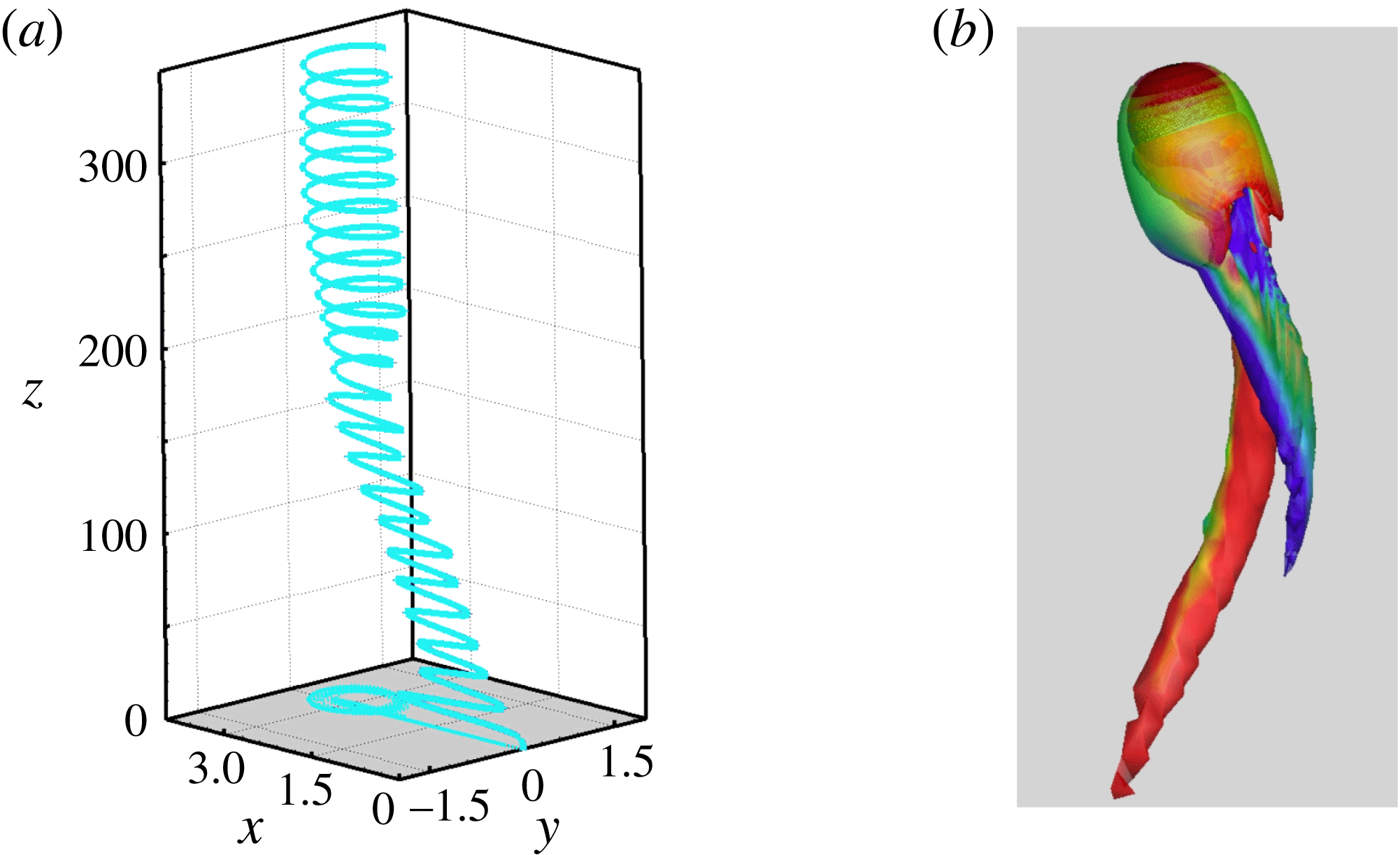
Figure 16. The spiralling (SP) regime for
 $\overline{\unicode[STIX]{x1D70C}}=0.01$
and
$\overline{\unicode[STIX]{x1D70C}}=0.01$
and
 $Ar=400$
. (a) Three-dimensional path (the horizontal projection of the path is displayed in the plane
$Ar=400$
. (a) Three-dimensional path (the horizontal projection of the path is displayed in the plane
 $z=0$
); (b) wake structure visualized with the
$z=0$
); (b) wake structure visualized with the
 $\unicode[STIX]{x1D706}_{2}$
criterion (
$\unicode[STIX]{x1D706}_{2}$
criterion (
 $-16.0\leqslant \unicode[STIX]{x1D714}_{z}\leqslant 14.5$
, see figure 4 for caption).
$-16.0\leqslant \unicode[STIX]{x1D714}_{z}\leqslant 14.5$
, see figure 4 for caption).
Using the refined grid described in § 2.3, we carried out a coarser exploration of the
 $(Ar,\overline{\unicode[STIX]{x1D70C}})$
plane from
$(Ar,\overline{\unicode[STIX]{x1D70C}})$
plane from
 $Ar=400$
to
$Ar=400$
to
 $Ar=700$
, especially to determine whether the SP regime identified at
$Ar=700$
, especially to determine whether the SP regime identified at
 $Ar=400$
exists over a significant parameter range or is rather an exception. To save CPU resources, only cases corresponding to
$Ar=400$
exists over a significant parameter range or is rather an exception. To save CPU resources, only cases corresponding to
 $Ar=500,600$
and
$Ar=500,600$
and
 $700$
were simulated and the solid-to-fluid density ratio
$700$
were simulated and the solid-to-fluid density ratio
 $\overline{\unicode[STIX]{x1D70C}}=0.001$
was omitted. Figure 17 shows how the path of a sphere with
$\overline{\unicode[STIX]{x1D70C}}=0.001$
was omitted. Figure 17 shows how the path of a sphere with
 $\overline{\unicode[STIX]{x1D70C}}=0.05$
varies from
$\overline{\unicode[STIX]{x1D70C}}=0.05$
varies from
 $Ar=375$
until
$Ar=375$
until
 $Ar=700$
. Premises of the SP regime are already present at
$Ar=700$
. Premises of the SP regime are already present at
 $Ar=375$
but no well-defined behaviour could be reached at that value of
$Ar=375$
but no well-defined behaviour could be reached at that value of
 $Ar$
(the same conclusion holds for both smaller and larger
$Ar$
(the same conclusion holds for both smaller and larger
 $\overline{\unicode[STIX]{x1D70C}}$
). In contrast, all paths obtained for
$\overline{\unicode[STIX]{x1D70C}}$
). In contrast, all paths obtained for
 $Ar\geqslant 400$
are seen to exhibit a clear spiralling structure. Most of the corresponding helices have a significant ellipticity, typically
$Ar\geqslant 400$
are seen to exhibit a clear spiralling structure. Most of the corresponding helices have a significant ellipticity, typically
 $1.5\pm 0.1:1$
, depending on
$1.5\pm 0.1:1$
, depending on
 $Ar$
. Some of them keep a vertical axis (i.e. the sphere rises vertically on average) but others do not. In particular, paths corresponding to
$Ar$
. Some of them keep a vertical axis (i.e. the sphere rises vertically on average) but others do not. In particular, paths corresponding to
 $Ar=500$
and
$Ar=500$
and
 $Ar=600$
contain a significant horizontal drift which may either keep a constant direction (
$Ar=600$
contain a significant horizontal drift which may either keep a constant direction (
 $Ar=600$
) or slowly rotate; in the latter case, the time-averaged path eventually describes an almost closed loop after a large number of periods of the primary helix (more than
$Ar=600$
) or slowly rotate; in the latter case, the time-averaged path eventually describes an almost closed loop after a large number of periods of the primary helix (more than
 $25$
for
$25$
for
 $Ar=500$
). Such paths, where a ‘slow’ periodic drift superimposes onto a ‘fast’ helical motion, are reminiscent of three-dimensional paths observed under certain conditions with falling disks in the fluttering or tumbling regimes (Auguste et al.
Reference Auguste, Magnaudet and Fabre2013). To appreciate how the domain of existence of the SP regime varies with
$Ar=500$
). Such paths, where a ‘slow’ periodic drift superimposes onto a ‘fast’ helical motion, are reminiscent of three-dimensional paths observed under certain conditions with falling disks in the fluttering or tumbling regimes (Auguste et al.
Reference Auguste, Magnaudet and Fabre2013). To appreciate how the domain of existence of the SP regime varies with
 $Ar$
, figure 18 shows the trajectories obtained for the various solid-to-fluid density ratios at
$Ar$
, figure 18 shows the trajectories obtained for the various solid-to-fluid density ratios at
 $Ar=700$
. All paths are fully chaotic and three-dimensional for spheres with
$Ar=700$
. All paths are fully chaotic and three-dimensional for spheres with
 $\overline{\unicode[STIX]{x1D70C}}>0.25$
. In contrast, after a long chaotic transient extending up to
$\overline{\unicode[STIX]{x1D70C}}>0.25$
. In contrast, after a long chaotic transient extending up to
 $z\approx 250$
, the sphere with
$z\approx 250$
, the sphere with
 $\overline{\unicode[STIX]{x1D70C}}=0.25$
starts to follow a clear, although not perfectly periodic, helical path. The remaining fluctuations discernible in the horizontal motion result in some meandering of the helix axis, and in some time-dependent variations of its ellipticity. As
$\overline{\unicode[STIX]{x1D70C}}=0.25$
starts to follow a clear, although not perfectly periodic, helical path. The remaining fluctuations discernible in the horizontal motion result in some meandering of the helix axis, and in some time-dependent variations of its ellipticity. As
 $\overline{\unicode[STIX]{x1D70C}}$
decreases, so does the relative magnitude of these fluctuations. The helical motion develops much more rapidly for
$\overline{\unicode[STIX]{x1D70C}}$
decreases, so does the relative magnitude of these fluctuations. The helical motion develops much more rapidly for
 $0.05\leqslant \overline{\unicode[STIX]{x1D70C}}\leqslant 0.175$
and the corresponding paths are close to perfectly circular helices. Surprisingly, as figure 18(b) reveals, the sphere with
$0.05\leqslant \overline{\unicode[STIX]{x1D70C}}\leqslant 0.175$
and the corresponding paths are close to perfectly circular helices. Surprisingly, as figure 18(b) reveals, the sphere with
 $\overline{\unicode[STIX]{x1D70C}}=0.01$
follows an almost planar zigzagging path with only a weak lateral drift over a long time, rather than a spiralling trajectory. Not unlikely, during that time, the wake structure is similar to that of figure 7, i.e. the shedding mode is of the ‘4R’ type, instead of the twisted vortex geometry displayed in figure 16. However the path geometry slowly evolves toward an elliptical helix with, in the last stages of the simulation, an aspect ratio somewhat less than 3 : 1. All dynamical characteristics recorded in that peculiar case are similar to those found throughout the SP regime: the Strouhal number is
$\overline{\unicode[STIX]{x1D70C}}=0.01$
follows an almost planar zigzagging path with only a weak lateral drift over a long time, rather than a spiralling trajectory. Not unlikely, during that time, the wake structure is similar to that of figure 7, i.e. the shedding mode is of the ‘4R’ type, instead of the twisted vortex geometry displayed in figure 16. However the path geometry slowly evolves toward an elliptical helix with, in the last stages of the simulation, an aspect ratio somewhat less than 3 : 1. All dynamical characteristics recorded in that peculiar case are similar to those found throughout the SP regime: the Strouhal number is
 $0.083$
(which corresponds to a maximum inclination of
$0.083$
(which corresponds to a maximum inclination of
 $24^{\circ }$
with respect to the vertical), and the crest-to-crest amplitude of lateral displacements is
$24^{\circ }$
with respect to the vertical), and the crest-to-crest amplitude of lateral displacements is
 ${\approx}1.9d$
, similar to the diameter of the helix observed for
${\approx}1.9d$
, similar to the diameter of the helix observed for
 $\overline{\unicode[STIX]{x1D70C}}=0.05$
; in the next section it will be shown that the drag coefficient also behaves similarly. Hence there is no doubt that this case belongs to the SP regime, although it exhibits a long transient with a specific path geometry (interestingly,
$\overline{\unicode[STIX]{x1D70C}}=0.05$
; in the next section it will be shown that the drag coefficient also behaves similarly. Hence there is no doubt that this case belongs to the SP regime, although it exhibits a long transient with a specific path geometry (interestingly,
 $Ar^{-1/2}\approx 0.038$
here, which according to § 3.1, makes this case with
$Ar^{-1/2}\approx 0.038$
here, which according to § 3.1, makes this case with
 $\overline{\unicode[STIX]{x1D70C}}=0.01$
the only one in which the sphere’s angular dynamics is controlled by viscous effects at
$\overline{\unicode[STIX]{x1D70C}}=0.01$
the only one in which the sphere’s angular dynamics is controlled by viscous effects at
 $Ar=700$
).
$Ar=700$
).
Figure 17. Path of a sphere with
 $\overline{\unicode[STIX]{x1D70C}}=0.05$
from
$\overline{\unicode[STIX]{x1D70C}}=0.05$
from
 $Ar=375$
to
$Ar=375$
to
 $Ar=700$
; (a) projection onto the vertical
$Ar=700$
; (a) projection onto the vertical
 $(x,z)$
plane, (b) projection onto the horizontal plane. Red:
$(x,z)$
plane, (b) projection onto the horizontal plane. Red:
 $Ar=375$
, green:
$Ar=375$
, green:
 $Ar=400$
, blue:
$Ar=400$
, blue:
 $Ar=500$
, purple:
$Ar=500$
, purple:
 $Ar=600$
, cyan:
$Ar=600$
, cyan:
 $Ar=700$
.
$Ar=700$
.
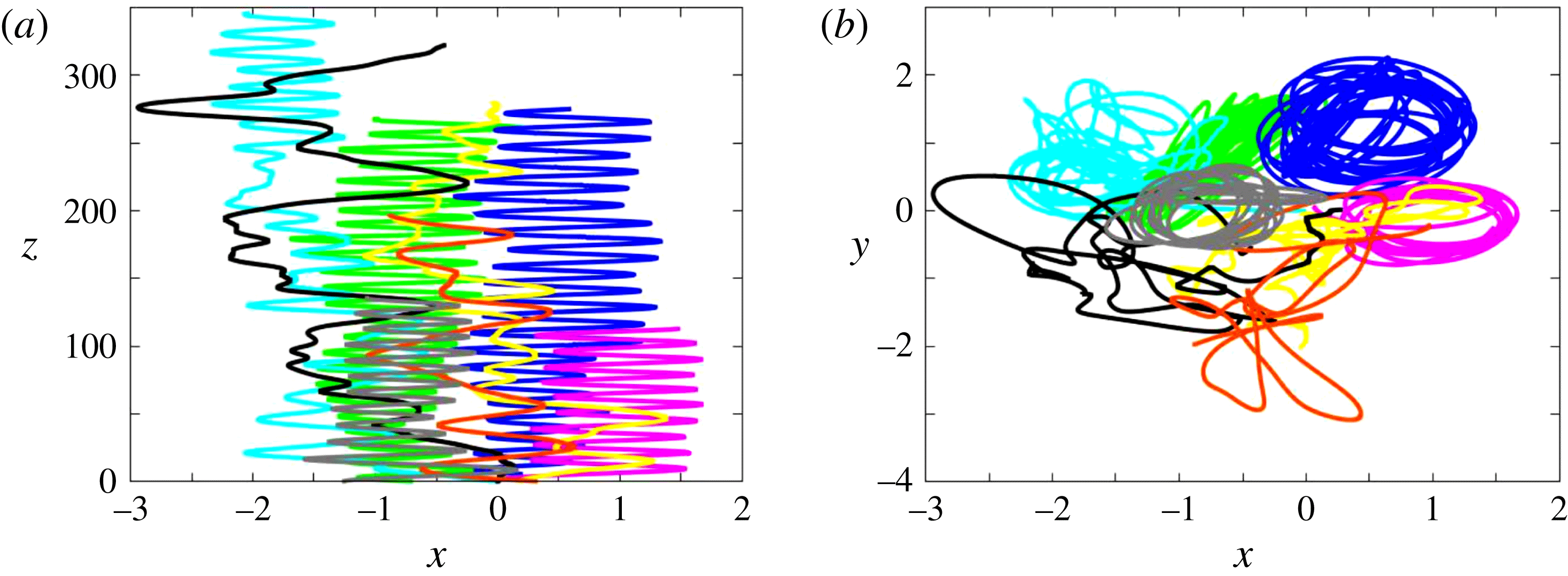
Figure 18. Paths for various solid-to-fluid density ratios at
 $Ar=700$
; (a) projection onto the vertical
$Ar=700$
; (a) projection onto the vertical
 $(x,z)$
plane, (b) projection onto the horizontal plane. Same colour code as in figure 6.
$(x,z)$
plane, (b) projection onto the horizontal plane. Same colour code as in figure 6.
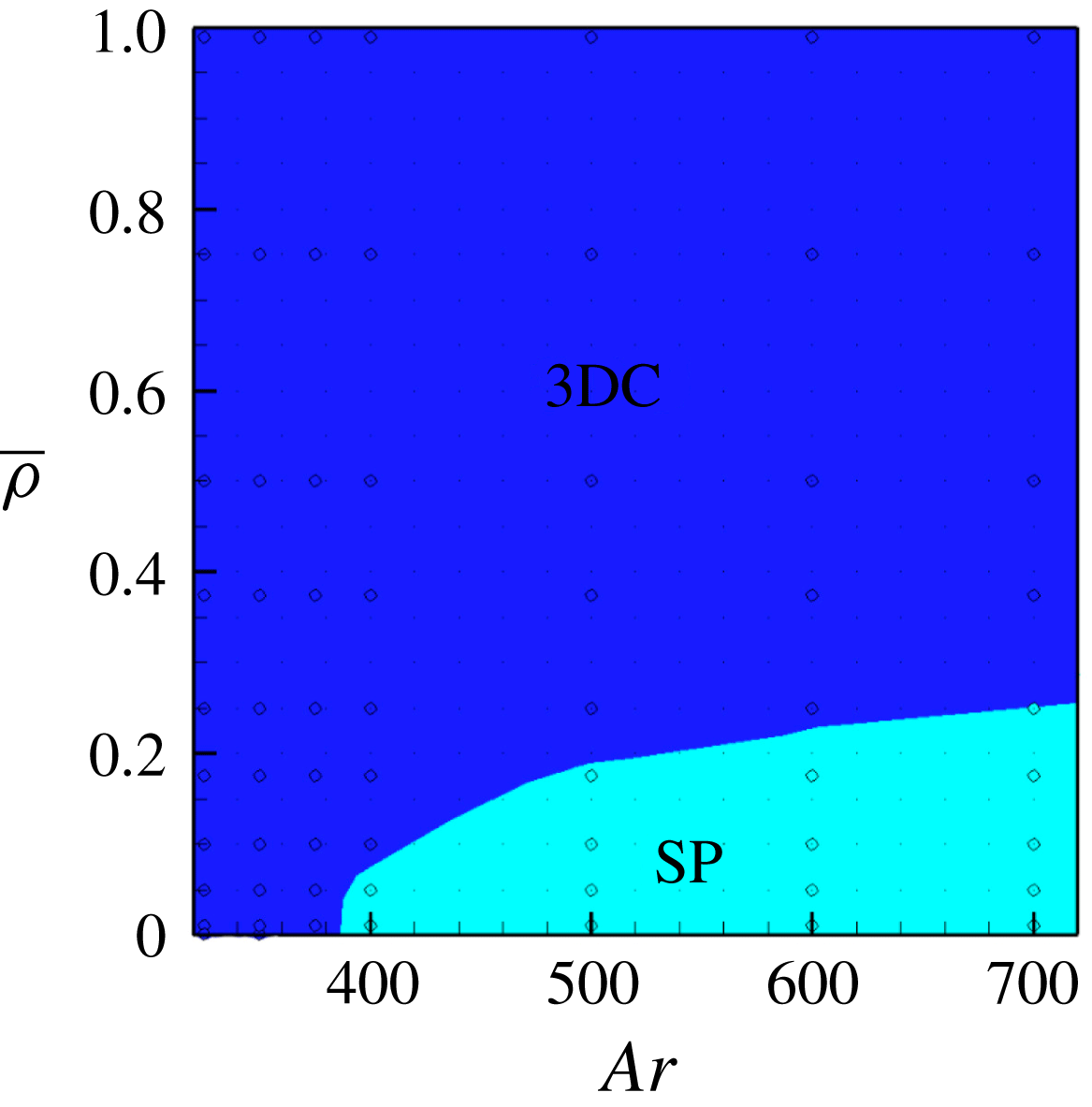
Figure 19. State diagram of rise regimes in the range
 $320\leqslant Ar\leqslant 700$
. Blue: three-dimensional chaotic (3DC); cyan: spiralling (SP).
$320\leqslant Ar\leqslant 700$
. Blue: three-dimensional chaotic (3DC); cyan: spiralling (SP).
The extent of the SP regime observed in present simulations is specified in figure 19 (the boundary between the 3DC and SP regimes was drawn without distinguishing between strictly periodic and ‘almost’ periodic helical paths). As this figure reveals, the maximum solid-to-fluid density ratio at which helical paths are observed sharply increases with
 $Ar$
, from
$Ar$
, from
 $0.05$
for
$0.05$
for
 $Ar=400$
to nearly
$Ar=400$
to nearly
 $0.25$
for
$0.25$
for
 $Ar=700$
. Throughout the SP regime, the diameter of the helices does not vary much and is always of the order of the sphere diameter. In contrast, for a given
$Ar=700$
. Throughout the SP regime, the diameter of the helices does not vary much and is always of the order of the sphere diameter. In contrast, for a given
 $\overline{\unicode[STIX]{x1D70C}}$
, their pitch decreases as
$\overline{\unicode[STIX]{x1D70C}}$
, their pitch decreases as
 $Ar$
increases, yielding increasing values of
$Ar$
increases, yielding increasing values of
 $St$
(e.g. for
$St$
(e.g. for
 $\overline{\unicode[STIX]{x1D70C}}=0.1$
, from
$\overline{\unicode[STIX]{x1D70C}}=0.1$
, from
 $St=0.058$
at
$St=0.058$
at
 $Ar=500$
to
$Ar=500$
to
 $St=0.085$
at
$St=0.085$
at
 $Ar=700$
). Similarly, for a given
$Ar=700$
). Similarly, for a given
 $Ar$
, the smaller
$Ar$
, the smaller
 $\overline{\unicode[STIX]{x1D70C}}$
, the shorter the pitch (i.e. the larger the inclination of the path with respect to the vertical), with for instance at
$\overline{\unicode[STIX]{x1D70C}}$
, the shorter the pitch (i.e. the larger the inclination of the path with respect to the vertical), with for instance at
 $Ar=700$
,
$Ar=700$
,
 $St=0.075$
for
$St=0.075$
for
 $\overline{\unicode[STIX]{x1D70C}}=0.25$
and
$\overline{\unicode[STIX]{x1D70C}}=0.25$
and
 $St=0.085$
for
$St=0.085$
for
 $\overline{\unicode[STIX]{x1D70C}}=0.1$
and
$\overline{\unicode[STIX]{x1D70C}}=0.1$
and
 $\overline{\unicode[STIX]{x1D70C}}=0.05$
. Circular helices with characteristics close to those discussed above were also identified by ZD in the range
$\overline{\unicode[STIX]{x1D70C}}=0.05$
. Circular helices with characteristics close to those discussed above were also identified by ZD in the range
 $375\leqslant Ar\leqslant 500$
for massless spheres (
$375\leqslant Ar\leqslant 500$
for massless spheres (
 $\overline{\unicode[STIX]{x1D70C}}=0$
), as well as in the case
$\overline{\unicode[STIX]{x1D70C}}=0$
), as well as in the case
 $\overline{\unicode[STIX]{x1D70C}}=0.1,Ar=500$
(
$\overline{\unicode[STIX]{x1D70C}}=0.1,Ar=500$
(
 $Ar=500$
was the upper limit considered in ZD’s simulations). Experiments reported in Veldhuis et al. (Reference Veldhuis, Biesheuvel and Lohse2009) also evidenced this type of trajectories for
$Ar=500$
was the upper limit considered in ZD’s simulations). Experiments reported in Veldhuis et al. (Reference Veldhuis, Biesheuvel and Lohse2009) also evidenced this type of trajectories for
 $\overline{\unicode[STIX]{x1D70C}}=0.02$
in the range
$\overline{\unicode[STIX]{x1D70C}}=0.02$
in the range
 $615\leqslant Ar\leqslant 875$
, the corresponding paths exhibiting a significant ellipticity (typically from 1.5 : 1 to 2 : 1). With
$615\leqslant Ar\leqslant 875$
, the corresponding paths exhibiting a significant ellipticity (typically from 1.5 : 1 to 2 : 1). With
 $Ar=615$
(their figure 2(a)), the Strouhal number was found to be
$Ar=615$
(their figure 2(a)), the Strouhal number was found to be
 $0.078$
, which compares very well with present findings which, at
$0.078$
, which compares very well with present findings which, at
 $Ar=600$
, indicate
$Ar=600$
, indicate
 $St=0.080$
for both
$St=0.080$
for both
 $\overline{\unicode[STIX]{x1D70C}}=0.05$
and
$\overline{\unicode[STIX]{x1D70C}}=0.05$
and
 $\overline{\unicode[STIX]{x1D70C}}=0.01$
. Interestingly, nearly perfect zigzags with Strouhal numbers about
$\overline{\unicode[STIX]{x1D70C}}=0.01$
. Interestingly, nearly perfect zigzags with Strouhal numbers about
 $0.085$
and crest-to-crest amplitudes about
$0.085$
and crest-to-crest amplitudes about
 $2d$
were observed in the same study, when
$2d$
were observed in the same study, when
 $Ar$
was increased up to
$Ar$
was increased up to
 $O(10^{3})$
values (see cases
$O(10^{3})$
values (see cases
 $d$
,
$d$
,
 $e$
in their figures 2 and 3). These characteristics are essentially those found in the specific case
$e$
in their figures 2 and 3). These characteristics are essentially those found in the specific case
 $Ar=700,\overline{\unicode[STIX]{x1D70C}}=0.01$
described above. Hence the whole set of observations presented above closely agree with the phenomenology reported in that experimental study.
$Ar=700,\overline{\unicode[STIX]{x1D70C}}=0.01$
described above. Hence the whole set of observations presented above closely agree with the phenomenology reported in that experimental study.
4 Drag
It has been repeatedly reported that, under certain conditions, the drag force experienced by a light sphere freely rising with an average vertical velocity
 $V_{m}$
in a fluid at rest may be significantly higher than that on a sphere held fixed in a uniform stream with upstream velocity
$V_{m}$
in a fluid at rest may be significantly higher than that on a sphere held fixed in a uniform stream with upstream velocity
 $-V_{m}$
. This question is usually assessed by equating the sphere’s net weight,
$-V_{m}$
. This question is usually assessed by equating the sphere’s net weight,
 $(\unicode[STIX]{x1D70C}_{s}-\unicode[STIX]{x1D70C})\unicode[STIX]{x03C0}d^{3}/6$
, to the drag force defined as
$(\unicode[STIX]{x1D70C}_{s}-\unicode[STIX]{x1D70C})\unicode[STIX]{x03C0}d^{3}/6$
, to the drag force defined as
 $C_{D}\unicode[STIX]{x03C0}\unicode[STIX]{x1D70C}d^{2}V_{m}^{2}/8$
, and comparing the drag coefficient,
$C_{D}\unicode[STIX]{x03C0}\unicode[STIX]{x1D70C}d^{2}V_{m}^{2}/8$
, and comparing the drag coefficient,
 $C_{D}(Re_{m})$
, to standard drag correlations. Although
$C_{D}(Re_{m})$
, to standard drag correlations. Although
 $C_{D}$
is known to decrease uniformly with
$C_{D}$
is known to decrease uniformly with
 $Re_{m}$
when the sphere is fixed (approximately as
$Re_{m}$
when the sphere is fixed (approximately as
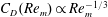 $C_{D}(Re_{m})\propto Re_{m}^{-1/3}$
for large enough
$C_{D}(Re_{m})\propto Re_{m}^{-1/3}$
for large enough
 $Re_{m}$
(Clift, Grace & Weber Reference Clift, Grace and Weber1978; Turton & Levenspiel Reference Turton and Levenspiel1986)), a series of experimental studies reported that sufficiently light spheres rising in a Newtonian liquid (Karamanev & Nikolov Reference Karamanev and Nikolov1992; Karamanev et al.
Reference Karamanev, Chavarie and Mayer1996) or soap bubbles rising in air (Karamanev Reference Karamanev2001) exhibit a drag coefficient close to
$Re_{m}$
(Clift, Grace & Weber Reference Clift, Grace and Weber1978; Turton & Levenspiel Reference Turton and Levenspiel1986)), a series of experimental studies reported that sufficiently light spheres rising in a Newtonian liquid (Karamanev & Nikolov Reference Karamanev and Nikolov1992; Karamanev et al.
Reference Karamanev, Chavarie and Mayer1996) or soap bubbles rising in air (Karamanev Reference Karamanev2001) exhibit a drag coefficient close to
 $0.95$
as soon as the Reynolds number exceeds a threshold value. The first (respectively second) study in this series identified a threshold Reynolds number close to
$0.95$
as soon as the Reynolds number exceeds a threshold value. The first (respectively second) study in this series identified a threshold Reynolds number close to
 $200$
(respectively
$200$
(respectively
 $380$
), and a maximum solid-to-fluid density ratio for such ‘abnormal’ drag coefficients to be observed of approximately
$380$
), and a maximum solid-to-fluid density ratio for such ‘abnormal’ drag coefficients to be observed of approximately
 $0.3$
(respectively
$0.3$
(respectively
 $0.7$
). However these results are questionable since most of them were obtained with non-homogeneous spheres, stainless steel rods having been inserted within expanded polystyrene spheres to vary their density. Although somewhat less spectacular, it was consistently observed by Horowitz & Williamson (Reference Horowitz and Williamson2010) that the drag coefficient of ‘vibrating’ (i.e. zigzagging) homogeneous spheres with
$0.7$
). However these results are questionable since most of them were obtained with non-homogeneous spheres, stainless steel rods having been inserted within expanded polystyrene spheres to vary their density. Although somewhat less spectacular, it was consistently observed by Horowitz & Williamson (Reference Horowitz and Williamson2010) that the drag coefficient of ‘vibrating’ (i.e. zigzagging) homogeneous spheres with
 $\overline{\unicode[STIX]{x1D70C}}\lesssim 0.36$
and
$\overline{\unicode[STIX]{x1D70C}}\lesssim 0.36$
and
 $Re_{m}\gtrsim 260$
takes a value of approximately
$Re_{m}\gtrsim 260$
takes a value of approximately
 $0.75$
which does not depend on
$0.75$
which does not depend on
 $Re_{m}$
any more. Among these light spheres, the authors noticed that ‘lighter spheres, which tend to have higher (oscillation) amplitudes, consistently exhibit greater drag’. A qualitatively similar behaviour was reported by Veldhuis et al. (Reference Veldhuis, Biesheuvel and Lohse2009) who found the drag coefficient of spiralling or zigzagging spheres with
$Re_{m}$
any more. Among these light spheres, the authors noticed that ‘lighter spheres, which tend to have higher (oscillation) amplitudes, consistently exhibit greater drag’. A qualitatively similar behaviour was reported by Veldhuis et al. (Reference Veldhuis, Biesheuvel and Lohse2009) who found the drag coefficient of spiralling or zigzagging spheres with
 $\overline{\unicode[STIX]{x1D70C}}=0.02$
to be close to
$\overline{\unicode[STIX]{x1D70C}}=0.02$
to be close to
 $0.85$
(
$0.85$
(
 $\pm 0.15$
) when
$\pm 0.15$
) when
 $Re_{m}\gtrsim 800$
, which is approximately 70 % higher than expected on the basis of standard drag correlations.
$Re_{m}\gtrsim 800$
, which is approximately 70 % higher than expected on the basis of standard drag correlations.
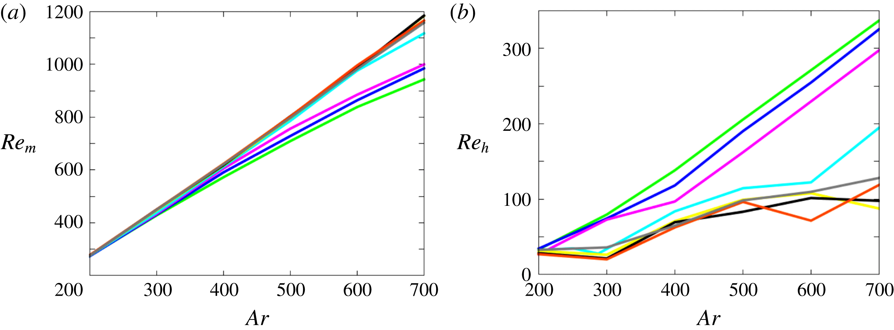
Figure 20. Variation of the sphere average rise velocity and root-mean-square velocity with the ratio of inertia to viscous effects, according to the sphere-to-fluid density ratio. (a) Average rise Reynolds number,
 $Re_{m}$
, versus the Archimedes number,
$Re_{m}$
, versus the Archimedes number,
 $Ar$
; (b) average Reynolds number of fluctuating motions,
$Ar$
; (b) average Reynolds number of fluctuating motions,
 $Re_{f}$
, versus
$Re_{f}$
, versus
 $Ar$
. The colour code is similar to that of figure 6 with the exception of the grey curve which refers to
$Ar$
. The colour code is similar to that of figure 6 with the exception of the grey curve which refers to
 $\overline{\unicode[STIX]{x1D70C}}=0.375$
.
$\overline{\unicode[STIX]{x1D70C}}=0.375$
.
Present computational results may be used to examine the behaviour of the average drag force as a function of
 $\overline{\unicode[STIX]{x1D70C}}$
and
$\overline{\unicode[STIX]{x1D70C}}$
and
 $Ar$
. For this purpose, we consider (2.6) at the end of each time step and average the vertical component of each term over time. Averaging is performed after removing the initial transient. In particular, when a well-defined regime (such as SO, PO, ZZ, ZO, ZZ
$Ar$
. For this purpose, we consider (2.6) at the end of each time step and average the vertical component of each term over time. Averaging is performed after removing the initial transient. In particular, when a well-defined regime (such as SO, PO, ZZ, ZO, ZZ
 $_{2}$
or SP) is reached after a long transient, the computed drag coefficient characterizes only this final regime. Assuming statistical stationarity, the averaging procedure removes contributions due to the instantaneous fluid and body accelerations, so that one is left with
$_{2}$
or SP) is reached after a long transient, the computed drag coefficient characterizes only this final regime. Assuming statistical stationarity, the averaging procedure removes contributions due to the instantaneous fluid and body accelerations, so that one is left with
 $\langle \boldsymbol{F}_{QS}(t)\rangle \boldsymbol{\cdot }\boldsymbol{e}_{\boldsymbol{z}}=(\unicode[STIX]{x1D70C}_{s}-\unicode[STIX]{x1D70C}){\mathcal{V}}g$
, where
$\langle \boldsymbol{F}_{QS}(t)\rangle \boldsymbol{\cdot }\boldsymbol{e}_{\boldsymbol{z}}=(\unicode[STIX]{x1D70C}_{s}-\unicode[STIX]{x1D70C}){\mathcal{V}}g$
, where
 $\boldsymbol{e}_{\boldsymbol{z}}=-\boldsymbol{g}/g$
stands for the unit vector in the vertical direction and
$\boldsymbol{e}_{\boldsymbol{z}}=-\boldsymbol{g}/g$
stands for the unit vector in the vertical direction and
 $\langle \,\boldsymbol{\cdot }\;\rangle$
denotes time-averaged quantities. Forming the dot product of (2.6) with
$\langle \,\boldsymbol{\cdot }\;\rangle$
denotes time-averaged quantities. Forming the dot product of (2.6) with
 $\boldsymbol{V}(t)$
and time averaging also removes contributions related to the instantaneous acceleration. Hence one also has
$\boldsymbol{V}(t)$
and time averaging also removes contributions related to the instantaneous acceleration. Hence one also has
 $\langle \boldsymbol{F}_{QS}(t)\boldsymbol{\cdot }\boldsymbol{V}(t)\rangle =(\unicode[STIX]{x1D70C}_{s}-\unicode[STIX]{x1D70C})g{\mathcal{V}}V_{m}$
, with
$\langle \boldsymbol{F}_{QS}(t)\boldsymbol{\cdot }\boldsymbol{V}(t)\rangle =(\unicode[STIX]{x1D70C}_{s}-\unicode[STIX]{x1D70C})g{\mathcal{V}}V_{m}$
, with
 $V_{m}=\langle \boldsymbol{V}(t)\rangle \boldsymbol{\cdot }\boldsymbol{e}_{\boldsymbol{z}}$
. The quantity
$V_{m}=\langle \boldsymbol{V}(t)\rangle \boldsymbol{\cdot }\boldsymbol{e}_{\boldsymbol{z}}$
. The quantity
 $\langle \boldsymbol{F}_{QS}(t)\boldsymbol{\cdot }\boldsymbol{V}(t)\rangle /V_{m}$
is the average drag force defined from a strict aerodynamic point of view (as it is built on the projection of the instantaneous force onto the instantaneous velocity), and comparison of the above two expressions shows that it is identical to the average of the vertical component of
$\langle \boldsymbol{F}_{QS}(t)\boldsymbol{\cdot }\boldsymbol{V}(t)\rangle /V_{m}$
is the average drag force defined from a strict aerodynamic point of view (as it is built on the projection of the instantaneous force onto the instantaneous velocity), and comparison of the above two expressions shows that it is identical to the average of the vertical component of
 $\boldsymbol{F}_{QS}(t)$
. One can thus define the time-averaged drag coefficient as
$\boldsymbol{F}_{QS}(t)$
. One can thus define the time-averaged drag coefficient as
 $\langle C_{D}\rangle =8\langle \boldsymbol{F}_{QS}\rangle \boldsymbol{\cdot }\boldsymbol{e}_{\boldsymbol{z}}/(\unicode[STIX]{x1D70C}\unicode[STIX]{x03C0}d^{2}V_{m}^{2})$
, so that the averaged vertical force balance writes
$\langle C_{D}\rangle =8\langle \boldsymbol{F}_{QS}\rangle \boldsymbol{\cdot }\boldsymbol{e}_{\boldsymbol{z}}/(\unicode[STIX]{x1D70C}\unicode[STIX]{x03C0}d^{2}V_{m}^{2})$
, so that the averaged vertical force balance writes
 $$\begin{eqnarray}\langle C_{D}\rangle (\overline{\unicode[STIX]{x1D70C}},\,Re_{m})Re_{m}^{2}={\textstyle \frac{4}{3}}Ar^{2}.\end{eqnarray}$$
Figure 20(a) shows how
 $Re_{m}$
varies with
$Re_{m}$
varies with
 $Ar$
for each solid-to-fluid density ratio. No significant influence of
$Ar$
for each solid-to-fluid density ratio. No significant influence of
 $\overline{\unicode[STIX]{x1D70C}}$
is discerned as far as
$\overline{\unicode[STIX]{x1D70C}}$
is discerned as far as
 $\overline{\unicode[STIX]{x1D70C}}\geqslant 0.375$
, since all curves almost superimpose. Note that in this range of
$\overline{\unicode[STIX]{x1D70C}}\geqslant 0.375$
, since all curves almost superimpose. Note that in this range of
 $\overline{\unicode[STIX]{x1D70C}}$
, the slope of these curves slightly increases with
$\overline{\unicode[STIX]{x1D70C}}$
, the slope of these curves slightly increases with
 $Ar$
in the right half of the figure. This is in line with the approximate
$Ar$
in the right half of the figure. This is in line with the approximate
 $\langle C_{D}\rangle \propto Re_{m}^{-1/3}$
large Reynolds number behaviour corresponding to fixed spheres in the range of
$\langle C_{D}\rangle \propto Re_{m}^{-1/3}$
large Reynolds number behaviour corresponding to fixed spheres in the range of
 $Re_{m}$
of interest here, which according to (4.1) yields
$Re_{m}$
of interest here, which according to (4.1) yields
 $Re_{m}\propto Ar^{6/5}$
. For lower
$Re_{m}\propto Ar^{6/5}$
. For lower
 $\overline{\unicode[STIX]{x1D70C}}$
, the average Reynolds number corresponding to a given
$\overline{\unicode[STIX]{x1D70C}}$
, the average Reynolds number corresponding to a given
 $Ar$
is seen to decrease in the high-
$Ar$
is seen to decrease in the high-
 $Ar$
range. This decrease is small and only takes place for
$Ar$
range. This decrease is small and only takes place for
 $Ar\gtrsim 600$
for
$Ar\gtrsim 600$
for
 $\overline{\unicode[STIX]{x1D70C}}=0.25$
. It is much more significant and emerges for
$\overline{\unicode[STIX]{x1D70C}}=0.25$
. It is much more significant and emerges for
 $Ar\approx 350$
for the lightest three spheres corresponding to
$Ar\approx 350$
for the lightest three spheres corresponding to
 $\overline{\unicode[STIX]{x1D70C}}\leqslant 0.1$
. Clearly, the domain within which the
$\overline{\unicode[STIX]{x1D70C}}\leqslant 0.1$
. Clearly, the domain within which the
 $Re_{m}-Ar$
relationship significantly depends on the sphere density essentially corresponds to the SP regime which appears to be the only one where path oscillations have a significant effect on the sphere drag. The connection between the decrease of the rise velocity and the increasing magnitude of the fluctuating motions is made clear by figure 20(b) which displays the Reynolds number,
$Re_{m}-Ar$
relationship significantly depends on the sphere density essentially corresponds to the SP regime which appears to be the only one where path oscillations have a significant effect on the sphere drag. The connection between the decrease of the rise velocity and the increasing magnitude of the fluctuating motions is made clear by figure 20(b) which displays the Reynolds number,
 $Re_{f}$
, based on the root-mean-square velocity,
$Re_{f}$
, based on the root-mean-square velocity,
 $V_{f}=\{\langle \boldsymbol{V}^{2}(t)\rangle -V_{m}^{2}\}^{1/2}$
(horizontal velocities associated with a possible non-zero mean drift are always very small, so that
$V_{f}=\{\langle \boldsymbol{V}^{2}(t)\rangle -V_{m}^{2}\}^{1/2}$
(horizontal velocities associated with a possible non-zero mean drift are always very small, so that
 $\langle \boldsymbol{V}(t)\rangle \approx V_{m}$
). As already mentioned, oscillations of very light spheres (those with
$\langle \boldsymbol{V}(t)\rangle \approx V_{m}$
). As already mentioned, oscillations of very light spheres (those with
 $\overline{\unicode[STIX]{x1D70C}}\leqslant 0.1$
) become significantly larger than those of heavier spheres in the 3DC regime; the lighter the sphere the more intense these oscillations. This tendency accentuates dramatically in the SP regime: while the ratio
$\overline{\unicode[STIX]{x1D70C}}\leqslant 0.1$
) become significantly larger than those of heavier spheres in the 3DC regime; the lighter the sphere the more intense these oscillations. This tendency accentuates dramatically in the SP regime: while the ratio
 $Re_{f}/Re_{m}$
stays in the range 10–12 % for all spheres with
$Re_{f}/Re_{m}$
stays in the range 10–12 % for all spheres with
 $\overline{\unicode[STIX]{x1D70C}}\geqslant 0.375$
, it rises beyond 30 % for those with
$\overline{\unicode[STIX]{x1D70C}}\geqslant 0.375$
, it rises beyond 30 % for those with
 $\overline{\unicode[STIX]{x1D70C}}\leqslant 0.1$
, reaching 35 % for the lightest one. These ratios demonstrate that a large fraction of the potential energy of the system ‘feeds’ the fluctuating motions of very light spheres rising in the SP regime, rather than their mean rising motion. Most of the kinetic energy
$\overline{\unicode[STIX]{x1D70C}}\leqslant 0.1$
, reaching 35 % for the lightest one. These ratios demonstrate that a large fraction of the potential energy of the system ‘feeds’ the fluctuating motions of very light spheres rising in the SP regime, rather than their mean rising motion. Most of the kinetic energy
 $V_{f}^{2}$
actually corresponds to horizontal motions whatever the style of path. In the ZZ regime, the vertical velocity fluctuation (normalized with
$V_{f}^{2}$
actually corresponds to horizontal motions whatever the style of path. In the ZZ regime, the vertical velocity fluctuation (normalized with
 $V_{m}$
) hardly exceeds 5 %, while the magnitude of the velocity fluctuation corresponding to a
$V_{m}$
) hardly exceeds 5 %, while the magnitude of the velocity fluctuation corresponding to a
 $1d$
-amplitude lateral excursion is
$1d$
-amplitude lateral excursion is
 $2\unicode[STIX]{x03C0}St$
. Hence, with
$2\unicode[STIX]{x03C0}St$
. Hence, with
 $St$
in the range 0.02–0.035, less than 15 % of
$St$
in the range 0.02–0.035, less than 15 % of
 $V_{f}^{2}$
is due to the vertical fluctuation. This is even more true in the SP regime, since the vertical velocity fluctuation is strictly zero in the case of a purely helical motion.
$V_{f}^{2}$
is due to the vertical fluctuation. This is even more true in the SP regime, since the vertical velocity fluctuation is strictly zero in the case of a purely helical motion.
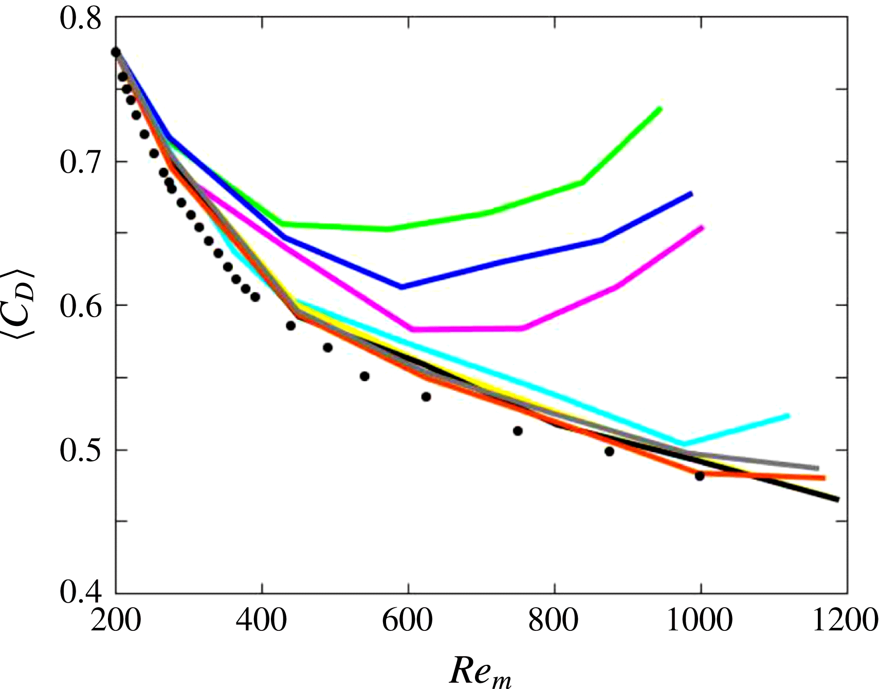
Figure 21. Average drag coefficient,
 $\langle C_{D}\rangle$
, versus the average Reynolds number,
$\langle C_{D}\rangle$
, versus the average Reynolds number,
 $Re_{m}$
. The colour code is similar to that of figure 20; closed circles indicate the drag coefficient for fixed spheres, obtained through computations performed with the standard (
$Re_{m}$
. The colour code is similar to that of figure 20; closed circles indicate the drag coefficient for fixed spheres, obtained through computations performed with the standard (
 $Re_{m}\leqslant 600$
) or refined (
$Re_{m}\leqslant 600$
) or refined (
 $Re_{m}>600$
) grid described in appendix B.
$Re_{m}>600$
) grid described in appendix B.
As figure 21 shows, the drag coefficient of freely rising spheres with
 $\overline{\unicode[STIX]{x1D70C}}>0.25$
is close to that computed for fixed spheres throughout the entire range of
$\overline{\unicode[STIX]{x1D70C}}>0.25$
is close to that computed for fixed spheres throughout the entire range of
 $Re_{m}$
, although generally somewhat larger for
$Re_{m}$
, although generally somewhat larger for
 $Re_{m}\gtrsim 300$
. This slight increase is due to nonlinear effects associated with velocity fluctuations
$Re_{m}\gtrsim 300$
. This slight increase is due to nonlinear effects associated with velocity fluctuations
 $\boldsymbol{V}(t)-V_{m}\boldsymbol{e}_{\boldsymbol{z}}$
, which affect the pressure and shear stress distributions at the sphere surface. In line with the above discussion, light spheres with
$\boldsymbol{V}(t)-V_{m}\boldsymbol{e}_{\boldsymbol{z}}$
, which affect the pressure and shear stress distributions at the sphere surface. In line with the above discussion, light spheres with
 $\overline{\unicode[STIX]{x1D70C}}\leqslant 0.1$
exhibit a different behaviour beyond
$\overline{\unicode[STIX]{x1D70C}}\leqslant 0.1$
exhibit a different behaviour beyond
 $Re_{m}\approx 350$
, i.e. as soon as they enter the 3DC regime: throughout that regime (which extends up to
$Re_{m}\approx 350$
, i.e. as soon as they enter the 3DC regime: throughout that regime (which extends up to
 $Re_{m}\approx 700$
(respectively
$Re_{m}\approx 700$
(respectively
 ${\approx}600$
) for
${\approx}600$
) for
 $\overline{\unicode[STIX]{x1D70C}}=0.1$
(respectively
$\overline{\unicode[STIX]{x1D70C}}=0.1$
(respectively
 $0.05$
and
$0.05$
and
 $0.01$
)), the corresponding
$0.01$
)), the corresponding
 $\langle C_{D}\rangle$
is significantly larger than that of heavier spheres, although it is still decreasing with increasing
$\langle C_{D}\rangle$
is significantly larger than that of heavier spheres, although it is still decreasing with increasing
 $Re_{m}$
. Then, a dramatic change is observed every time a light sphere enters the SP regime: since that point, the drag coefficient increases with the Reynolds number, a trend in stark contrast with its usual behaviour. Maximum drag coefficients about
$Re_{m}$
. Then, a dramatic change is observed every time a light sphere enters the SP regime: since that point, the drag coefficient increases with the Reynolds number, a trend in stark contrast with its usual behaviour. Maximum drag coefficients about
 $0.75$
are found with the lightest spheres for
$0.75$
are found with the lightest spheres for
 $Re_{m}\approx 10^{3}$
, which represents a 50 % increase compared to values found at the same
$Re_{m}\approx 10^{3}$
, which represents a 50 % increase compared to values found at the same
 $Re_{m}$
for spheres with
$Re_{m}$
for spheres with
 $\overline{\unicode[STIX]{x1D70C}}\geqslant 0.375$
. Although this is somewhat less than the average value determined by Veldhuis et al. (Reference Veldhuis, Biesheuvel and Lohse2009),
$\overline{\unicode[STIX]{x1D70C}}\geqslant 0.375$
. Although this is somewhat less than the average value determined by Veldhuis et al. (Reference Veldhuis, Biesheuvel and Lohse2009),
 $\langle C_{D}\rangle \approx 0.85\pm 0.15$
, the connection is clear, both in terms of the Reynolds number range and magnitude of the departure from standard behaviour. It is unfortunate that the sphere-to-fluid density ratio directly jumped from
$\langle C_{D}\rangle \approx 0.85\pm 0.15$
, the connection is clear, both in terms of the Reynolds number range and magnitude of the departure from standard behaviour. It is unfortunate that the sphere-to-fluid density ratio directly jumped from
 $0.02$
to
$0.02$
to
 $0.85$
in those experiments, preventing any estimate of the maximum
$0.85$
in those experiments, preventing any estimate of the maximum
 $\overline{\unicode[STIX]{x1D70C}}$
at which this non-standard behaviour takes place. A similar connection might exist with the behaviour of ‘vibrating’ spheres observed by Horowitz & Williamson (Reference Horowitz and Williamson2010). However it is much less clear because the corresponding paths were reported to be strictly planar (see their figure 9). In Veldhuis et al. (Reference Veldhuis, Biesheuvel and Lohse2009), spiralling and zigzagging spheres with
$\overline{\unicode[STIX]{x1D70C}}$
at which this non-standard behaviour takes place. A similar connection might exist with the behaviour of ‘vibrating’ spheres observed by Horowitz & Williamson (Reference Horowitz and Williamson2010). However it is much less clear because the corresponding paths were reported to be strictly planar (see their figure 9). In Veldhuis et al. (Reference Veldhuis, Biesheuvel and Lohse2009), spiralling and zigzagging spheres with
 $\overline{\unicode[STIX]{x1D70C}}=0.02$
and
$\overline{\unicode[STIX]{x1D70C}}=0.02$
and
 $Re_{m}\gtrsim 800$
were all found to have similar drag coefficients. Here, as we saw in § 3.4, all spheres standing in the SP regime are spiralling. Nevertheless, the spiral aspect ratio was noticed to be large in the case
$Re_{m}\gtrsim 800$
were all found to have similar drag coefficients. Here, as we saw in § 3.4, all spheres standing in the SP regime are spiralling. Nevertheless, the spiral aspect ratio was noticed to be large in the case
 $Ar=700,\,\overline{\unicode[STIX]{x1D70C}}=0.01$
corresponding to the rightmost point on the green curve in figure 20. The associated
$Ar=700,\,\overline{\unicode[STIX]{x1D70C}}=0.01$
corresponding to the rightmost point on the green curve in figure 20. The associated
 $\langle C_{D}\rangle$
turns out to be the largest reached in the present investigation and the corresponding value,
$\langle C_{D}\rangle$
turns out to be the largest reached in the present investigation and the corresponding value,
 $\langle C_{D}\rangle =0.74$
, is virtually identical to the average drag coefficients measured by Horowitz & Williamson (Reference Horowitz and Williamson2010) for ‘vibrating’ spheres, namely
$\langle C_{D}\rangle =0.74$
, is virtually identical to the average drag coefficients measured by Horowitz & Williamson (Reference Horowitz and Williamson2010) for ‘vibrating’ spheres, namely
 $\langle C_{D}\rangle =0.75$
. These similarities leave the possibility for a connection between their findings and present predictions open. However one has to keep in mind that they detected this ‘non-standard’ behaviour for all spheres with
$\langle C_{D}\rangle =0.75$
. These similarities leave the possibility for a connection between their findings and present predictions open. However one has to keep in mind that they detected this ‘non-standard’ behaviour for all spheres with
 $\overline{\unicode[STIX]{x1D70C}}\leqslant 0.36$
provided that the Reynolds number is larger than
$\overline{\unicode[STIX]{x1D70C}}\leqslant 0.36$
provided that the Reynolds number is larger than
 $260$
, which is drastically different from what is observed here. A noticeable difference between the present
$260$
, which is drastically different from what is observed here. A noticeable difference between the present
 $C_{D}=f(Re_{m})$
curves obtained with light spheres and the behaviour observed by Veldhuis et al. for spheres with
$C_{D}=f(Re_{m})$
curves obtained with light spheres and the behaviour observed by Veldhuis et al. for spheres with
 $\overline{\unicode[STIX]{x1D70C}}=0.02$
is that no tendency for
$\overline{\unicode[STIX]{x1D70C}}=0.02$
is that no tendency for
 $C_{D}$
to become constant beyond a certain Reynolds number emerges from figure 21. However, only data corresponding to
$C_{D}$
to become constant beyond a certain Reynolds number emerges from figure 21. However, only data corresponding to
 $Ar=600$
and
$Ar=600$
and
 $Ar=700$
with
$Ar=700$
with
 $\overline{\unicode[STIX]{x1D70C}}=0.01$
fall within the region where this ‘plateau’ was experimentally observed. Therefore it may well be that the overlap between experimental and computational data is just too narrow to allow this remarkable behaviour to emerge from the computations. Only new runs performed on finer grids at higher
$\overline{\unicode[STIX]{x1D70C}}=0.01$
fall within the region where this ‘plateau’ was experimentally observed. Therefore it may well be that the overlap between experimental and computational data is just too narrow to allow this remarkable behaviour to emerge from the computations. Only new runs performed on finer grids at higher
 $Ar$
may clarify this point.
$Ar$
may clarify this point.

5 Discussion and concluding remarks
5.1 Overview of rise regimes
Figure 22 obtained by merging figures 2, 13 and 19, displays all rise regimes observed throughout this study. It helps make a global assessment of the influence of the sphere-to-fluid density ratio on the flow and path transitions up to
 $Ar=700$
. Note that in some cases, paths on which this regime map is based might not reflect the ultimate sphere trajectory (e.g. the late intermittency observed for
$Ar=700$
. Note that in some cases, paths on which this regime map is based might not reflect the ultimate sphere trajectory (e.g. the late intermittency observed for
 $\overline{\unicode[STIX]{x1D70C}}=0.1$
in figure 5 or the late switching to the ZZ
$\overline{\unicode[STIX]{x1D70C}}=0.1$
in figure 5 or the late switching to the ZZ
 $_{2}$
regime for
$_{2}$
regime for
 $\overline{\unicode[STIX]{x1D70C}}=0.99$
in figure 11). Although they only represent very long transients in such cases, they are relevant for comparison with available laboratory observations which were all carried out in tanks of limited height, with height-to-sphere diameter ratios of some hundreds (400 and 500 for the smallest spheres in Veldhuis & Biesheuvel (Reference Veldhuis and Biesheuvel2007) and Horowitz & Williamson (Reference Horowitz and Williamson2010), respectively).
$\overline{\unicode[STIX]{x1D70C}}=0.99$
in figure 11). Although they only represent very long transients in such cases, they are relevant for comparison with available laboratory observations which were all carried out in tanks of limited height, with height-to-sphere diameter ratios of some hundreds (400 and 500 for the smallest spheres in Veldhuis & Biesheuvel (Reference Veldhuis and Biesheuvel2007) and Horowitz & Williamson (Reference Horowitz and Williamson2010), respectively).
Increasing
 $Ar$
from an
$Ar$
from an
 $O(10^{2})$
value, all spheres successively pass through the SV, SO and PO regimes, and the latter is always succeeded by an intermittent regime spanning a narrow
$O(10^{2})$
value, all spheres successively pass through the SV, SO and PO regimes, and the latter is always succeeded by an intermittent regime spanning a narrow
 $Ar$
range. Then the ‘life’ of spheres becomes dramatically dependent on
$Ar$
range. Then the ‘life’ of spheres becomes dramatically dependent on
 $\overline{\unicode[STIX]{x1D70C}}$
. Basically, those with
$\overline{\unicode[STIX]{x1D70C}}$
. Basically, those with
 $\overline{\unicode[STIX]{x1D70C}}\gtrsim 0.6$
reach the 3DC state through a succession of two periodic regimes corresponding to zigzagging paths with markedly distinct characteristics, planar large-amplitude low-frequency ZZ paths being succeeded by three-dimensional small-amplitude high-frequency ZZ
$\overline{\unicode[STIX]{x1D70C}}\gtrsim 0.6$
reach the 3DC state through a succession of two periodic regimes corresponding to zigzagging paths with markedly distinct characteristics, planar large-amplitude low-frequency ZZ paths being succeeded by three-dimensional small-amplitude high-frequency ZZ
 $_{2}$
paths. Spheres with intermediate density ratios, say
$_{2}$
paths. Spheres with intermediate density ratios, say
 $0.2\lesssim \overline{\unicode[STIX]{x1D70C}}\lesssim 0.6$
, follow somewhat more complicated routes with an intermediate intermittent regime (with planar paths up to
$0.2\lesssim \overline{\unicode[STIX]{x1D70C}}\lesssim 0.6$
, follow somewhat more complicated routes with an intermediate intermittent regime (with planar paths up to
 $Ar\approx 235$
and three-dimensional paths beyond that threshold) separating the ZZ and ZZ
$Ar\approx 235$
and three-dimensional paths beyond that threshold) separating the ZZ and ZZ
 $_{2}$
regimes if
$_{2}$
regimes if
 $\overline{\unicode[STIX]{x1D70C}}\gtrsim 0.3$
, and a direct transition from the three-dimensional region of this IT regime to the 3DC state without any ZZ
$\overline{\unicode[STIX]{x1D70C}}\gtrsim 0.3$
, and a direct transition from the three-dimensional region of this IT regime to the 3DC state without any ZZ
 $_{2}$
range if
$_{2}$
range if
 $\overline{\unicode[STIX]{x1D70C}}\lesssim 0.3$
. Obviously the behaviour of very light spheres (say with
$\overline{\unicode[STIX]{x1D70C}}\lesssim 0.3$
. Obviously the behaviour of very light spheres (say with
 $\overline{\unicode[STIX]{x1D70C}}\lesssim 0.2$
) is by far the richest. Increasing
$\overline{\unicode[STIX]{x1D70C}}\lesssim 0.2$
) is by far the richest. Increasing
 $Ar$
from the first IT stripe ending at
$Ar$
from the first IT stripe ending at
 $Ar\approx 175$
, one first encounters a ZZ range which becomes very narrow as
$Ar\approx 175$
, one first encounters a ZZ range which becomes very narrow as
 $\overline{\unicode[STIX]{x1D70C}}\rightarrow 0$
. It is followed by a transition region, the detailed shape of which strongly depends on
$\overline{\unicode[STIX]{x1D70C}}\rightarrow 0$
. It is followed by a transition region, the detailed shape of which strongly depends on
 $\overline{\unicode[STIX]{x1D70C}}$
, dominated by planar oblique zigzagging paths. These paths develop, first intermittently, then in a uniform manner for slightly larger
$\overline{\unicode[STIX]{x1D70C}}$
, dominated by planar oblique zigzagging paths. These paths develop, first intermittently, then in a uniform manner for slightly larger
 $Ar$
, yielding the ZO periodic regime. Intermittent two- or three-dimensional oblique zigzags succeed this specific periodic regime (depending on the highest
$Ar$
, yielding the ZO periodic regime. Intermittent two- or three-dimensional oblique zigzags succeed this specific periodic regime (depending on the highest
 $Ar$
at which it stops for the considered
$Ar$
at which it stops for the considered
 $\overline{\unicode[STIX]{x1D70C}}$
) before the system reaches the 3DC state. Last, a new ordered state emerges in the form of the SP regime characterized by paths with large-amplitude horizontal displacements associated with a Strouhal number of approximately
$\overline{\unicode[STIX]{x1D70C}}$
) before the system reaches the 3DC state. Last, a new ordered state emerges in the form of the SP regime characterized by paths with large-amplitude horizontal displacements associated with a Strouhal number of approximately
 $0.08$
. Paths in that regime are spiralling, with circular or elliptical horizontal projections (with ellipticity ratios up to 3 : 1), sometimes reached after a long nearly planar zigzagging transient.
$0.08$
. Paths in that regime are spiralling, with circular or elliptical horizontal projections (with ellipticity ratios up to 3 : 1), sometimes reached after a long nearly planar zigzagging transient.
5.2 Comparison with available results
Some partial comparison between the above findings and available computational and experimental results was performed in the course of §§ 3 and 4. However a more global discussion is in order to identify the points of consensus and disagreement that have been reached.
Starting with computations, to the best of our knowledge, only JDB and ZD dealt in detail with this problem. Present findings are in good agreement with those reported in these two studies up to
 $Ar\approx 175$
for
$Ar\approx 175$
for
 $\overline{\unicode[STIX]{x1D70C}}\approx 0$
and
$\overline{\unicode[STIX]{x1D70C}}\approx 0$
and
 $Ar\approx 190$
for
$Ar\approx 190$
for
 $\overline{\unicode[STIX]{x1D70C}}\approx 1$
, which corresponds to the upper limit of the periodic oscillating (PO) regime. Only some minor differences were noticed regarding the
$\overline{\unicode[STIX]{x1D70C}}\approx 1$
, which corresponds to the upper limit of the periodic oscillating (PO) regime. Only some minor differences were noticed regarding the
 $Ar$
threshold at the SO–PO transition. All three studies also conclude that the onset of chaos in the present system takes place at the upper bound of the PO regime. In the opposite limit, say
$Ar$
threshold at the SO–PO transition. All three studies also conclude that the onset of chaos in the present system takes place at the upper bound of the PO regime. In the opposite limit, say
 $Ar>300$
, our results and those of ZD also yield converging conclusions (JDB’s investigation was limited to
$Ar>300$
, our results and those of ZD also yield converging conclusions (JDB’s investigation was limited to
 $Ar=350$
). That is, both studies predict that all spheres follow chaotic three-dimensional paths, except those corresponding to very small
$Ar=350$
). That is, both studies predict that all spheres follow chaotic three-dimensional paths, except those corresponding to very small
 $\overline{\unicode[STIX]{x1D70C}}$
which exhibit spiralling paths for large enough
$\overline{\unicode[STIX]{x1D70C}}$
which exhibit spiralling paths for large enough
 $Ar$
. Here also the thresholds are only slightly different: ZD detected the onset of the SP regime at
$Ar$
. Here also the thresholds are only slightly different: ZD detected the onset of the SP regime at
 $Ar=375$
for
$Ar=375$
for
 $\overline{\unicode[STIX]{x1D70C}}=0.0$
while we only observe it for
$\overline{\unicode[STIX]{x1D70C}}=0.0$
while we only observe it for
 $Ar\geqslant 400$
. No comparison can be performed regarding the extent of the SP subdomain, since ZD did not consider solid-to-fluid density ratios intermediate between
$Ar\geqslant 400$
. No comparison can be performed regarding the extent of the SP subdomain, since ZD did not consider solid-to-fluid density ratios intermediate between
 $\overline{\unicode[STIX]{x1D70C}}=0.0$
and
$\overline{\unicode[STIX]{x1D70C}}=0.0$
and
 $\overline{\unicode[STIX]{x1D70C}}=0.2$
, except for
$\overline{\unicode[STIX]{x1D70C}}=0.2$
, except for
 $Ar=500$
where they also observed a helical path for
$Ar=500$
where they also observed a helical path for
 $\overline{\unicode[STIX]{x1D70C}}=0.1$
. At
$\overline{\unicode[STIX]{x1D70C}}=0.1$
. At
 $Ar=500$
, they reported drag coefficients of
$Ar=500$
, they reported drag coefficients of
 $0.67$
and
$0.67$
and
 $0.59$
for
$0.59$
for
 $\overline{\unicode[STIX]{x1D70C}}=0.0$
and
$\overline{\unicode[STIX]{x1D70C}}=0.0$
and
 $\overline{\unicode[STIX]{x1D70C}}=0.1$
, respectively. These values compare well with present findings, namely
$\overline{\unicode[STIX]{x1D70C}}=0.1$
, respectively. These values compare well with present findings, namely
 $\langle C_{D}\rangle =0.654$
and
$\langle C_{D}\rangle =0.654$
and
 $0.598$
for
$0.598$
for
 $\overline{\unicode[STIX]{x1D70C}}=0.01$
and
$\overline{\unicode[STIX]{x1D70C}}=0.01$
and
 $\overline{\unicode[STIX]{x1D70C}}=0.1$
, respectively.
$\overline{\unicode[STIX]{x1D70C}}=0.1$
, respectively.
The situation is more complex in the intermediate
 $Ar$
range, i.e. in between the PO and 3DC regimes. Roughly speaking, ZD found that a vast majority of the
$Ar$
range, i.e. in between the PO and 3DC regimes. Roughly speaking, ZD found that a vast majority of the
 $(Ar,\,\overline{\unicode[STIX]{x1D70C}})$
combinations in that range corresponds to chaotic regimes, with a few exceptions associated with periodic paths. Most of the latter belong to two disconnected subdomains, namely that of large-amplitude planar zigzags extending up to
$(Ar,\,\overline{\unicode[STIX]{x1D70C}})$
combinations in that range corresponds to chaotic regimes, with a few exceptions associated with periodic paths. Most of the latter belong to two disconnected subdomains, namely that of large-amplitude planar zigzags extending up to
 $\overline{\unicode[STIX]{x1D70C}}\approx 0.5$
for
$\overline{\unicode[STIX]{x1D70C}}\approx 0.5$
for
 $180\lesssim Ar\lesssim 200$
, and that of ‘vertical oscillating’ paths extending beyond
$180\lesssim Ar\lesssim 200$
, and that of ‘vertical oscillating’ paths extending beyond
 $\overline{\unicode[STIX]{x1D70C}}\approx 0.5$
in the range
$\overline{\unicode[STIX]{x1D70C}}\approx 0.5$
in the range
 $250\lesssim Ar\lesssim 300$
. This contrasts with the large subdomains corresponding to periodic regimes in figure 22, especially for
$250\lesssim Ar\lesssim 300$
. This contrasts with the large subdomains corresponding to periodic regimes in figure 22, especially for
 $\overline{\unicode[STIX]{x1D70C}}\geqslant 0.35$
where the planar ZZ regime and the three-dimensional ZZ
$\overline{\unicode[STIX]{x1D70C}}\geqslant 0.35$
where the planar ZZ regime and the three-dimensional ZZ
 $_{2}$
regime dominate the scene. Even for lower
$_{2}$
regime dominate the scene. Even for lower
 $\overline{\unicode[STIX]{x1D70C}}$
, the ZZ regime still spans a substantial range of
$\overline{\unicode[STIX]{x1D70C}}$
, the ZZ regime still spans a substantial range of
 $Ar$
down to
$Ar$
down to
 $\overline{\unicode[STIX]{x1D70C}}\approx 0.15$
and the ZO regime represents a well-identified, albeit small, island of periodicity for low
$\overline{\unicode[STIX]{x1D70C}}\approx 0.15$
and the ZO regime represents a well-identified, albeit small, island of periodicity for low
 $\overline{\unicode[STIX]{x1D70C}}$
, which contrasts with ZD’s results in which only two isolated points were found to correspond to a ‘fast oblique zigzagging’ regime for
$\overline{\unicode[STIX]{x1D70C}}$
, which contrasts with ZD’s results in which only two isolated points were found to correspond to a ‘fast oblique zigzagging’ regime for
 $\overline{\unicode[STIX]{x1D70C}}\leqslant 0.2$
. At this stage, it must be mentioned that in this intermediate
$\overline{\unicode[STIX]{x1D70C}}\leqslant 0.2$
. At this stage, it must be mentioned that in this intermediate
 $Ar$
range, the regime map provided by ZD for
$Ar$
range, the regime map provided by ZD for
 $\overline{\unicode[STIX]{x1D70C}}<1$
is quite different from JDB’s original map, although both studies were carried out with the same code. Some of these differences may be attributed to the longer physical times reached in ZD’s simulations but the origin of others is less clear and presumably results from small changes between the two versions of the code. The most remarkable of these differences is the extent of the domain corresponding to the ZZ regime, which turns out to be much larger in JDB, where this type of path was observed up to
$\overline{\unicode[STIX]{x1D70C}}<1$
is quite different from JDB’s original map, although both studies were carried out with the same code. Some of these differences may be attributed to the longer physical times reached in ZD’s simulations but the origin of others is less clear and presumably results from small changes between the two versions of the code. The most remarkable of these differences is the extent of the domain corresponding to the ZZ regime, which turns out to be much larger in JDB, where this type of path was observed up to
 $\overline{\unicode[STIX]{x1D70C}}\approx 1$
within the range
$\overline{\unicode[STIX]{x1D70C}}\approx 1$
within the range
 $200\lesssim Ar\lesssim 215$
. Even for lighter spheres, the
$200\lesssim Ar\lesssim 215$
. Even for lighter spheres, the
 $Ar$
stripe corresponding to the ZZ regime is much broader in JDB: for
$Ar$
stripe corresponding to the ZZ regime is much broader in JDB: for
 $\overline{\unicode[STIX]{x1D70C}}=0.2$
it spans the range
$\overline{\unicode[STIX]{x1D70C}}=0.2$
it spans the range
 $175\leqslant Ar\lesssim 200$
, while it is restricted to the narrow interval
$175\leqslant Ar\lesssim 200$
, while it is restricted to the narrow interval
 $175\lesssim Ar\lesssim 182$
in ZD. Considering figure 22, it is clear that our results are in much better agreement with those of JDB in that respect; nevertheless, the ZZ regime subsists up to
$175\lesssim Ar\lesssim 182$
in ZD. Considering figure 22, it is clear that our results are in much better agreement with those of JDB in that respect; nevertheless, the ZZ regime subsists up to
 $Ar\approx 250$
when
$Ar\approx 250$
when
 $\overline{\unicode[STIX]{x1D70C}}\gtrsim 0.6$
in our computations, while JDB reported three-dimensional chaotic paths beyond
$\overline{\unicode[STIX]{x1D70C}}\gtrsim 0.6$
in our computations, while JDB reported three-dimensional chaotic paths beyond
 $Ar\approx 215$
in that range of
$Ar\approx 215$
in that range of
 $\overline{\unicode[STIX]{x1D70C}}$
. Another difference between JDB’s and ZD’s conclusions stands in the area of coexistence of the 3DC regime with the ‘vertical oscillating’ regime, which JDB found to take place within a wide region covering approximately
$\overline{\unicode[STIX]{x1D70C}}$
. Another difference between JDB’s and ZD’s conclusions stands in the area of coexistence of the 3DC regime with the ‘vertical oscillating’ regime, which JDB found to take place within a wide region covering approximately
 $60$
$60$
 $Ar$
-units for
$Ar$
-units for
 $\overline{\unicode[STIX]{x1D70C}}=0.0$
and broadening up to
$\overline{\unicode[STIX]{x1D70C}}=0.0$
and broadening up to
 $100$
$100$
 $Ar$
-units for
$Ar$
-units for
 $\overline{\unicode[STIX]{x1D70C}}=1.0$
, while it was only observed at
$\overline{\unicode[STIX]{x1D70C}}=1.0$
, while it was only observed at
 $Ar=250$
and
$Ar=250$
and
 $260$
for
$260$
for
 $\overline{\unicode[STIX]{x1D70C}}=1.0$
by ZD: by running simulations over much longer times, the latter study could exclude most cases of bi-stability identified or suspected by JDB. Despite several attempts to disturb ZZ
$\overline{\unicode[STIX]{x1D70C}}=1.0$
by ZD: by running simulations over much longer times, the latter study could exclude most cases of bi-stability identified or suspected by JDB. Despite several attempts to disturb ZZ
 $_{2}$
paths or to modify initial conditions in the range where they are seen to exist in figure 22, we never observed any indication of bi-stability close to the ZZ
$_{2}$
paths or to modify initial conditions in the range where they are seen to exist in figure 22, we never observed any indication of bi-stability close to the ZZ
 $_{2}$
–3DC boundary; in contrast we noticed some sporadic switches to the ZZ regime close to the ZZ–ZZ
$_{2}$
–3DC boundary; in contrast we noticed some sporadic switches to the ZZ regime close to the ZZ–ZZ
 $_{2}$
boundary, which might correspond to the small area of bi-stability detected by ZD. Last but not least, we stress again that the periodic ZZ
$_{2}$
boundary, which might correspond to the small area of bi-stability detected by ZD. Last but not least, we stress again that the periodic ZZ
 $_{2}$
and ZO regimes observed here exhibit structural differences with, respectively, the ‘vertical oscillating’ and ‘fast oblique zigzagging’ regimes described in ZD, although their domains of existence coincide (for ZZ
$_{2}$
and ZO regimes observed here exhibit structural differences with, respectively, the ‘vertical oscillating’ and ‘fast oblique zigzagging’ regimes described in ZD, although their domains of existence coincide (for ZZ
 $_{2}$
) or suggest a close connection (for ZO). Indeed we found the former to exhibit significant three-dimensional features (the only exception is the path corresponding to
$_{2}$
) or suggest a close connection (for ZO). Indeed we found the former to exhibit significant three-dimensional features (the only exception is the path corresponding to
 $\overline{\unicode[STIX]{x1D70C}}=0.99$
in figure 11) and a non-zero in-plane lateral drift, while ZD insisted on the ‘remarkably accurate planarity and verticality’ of the ‘vertical oscillating’ regime. Conversely, ZO paths stand in strictly vertical planes and correspond to low-frequency oscillations (with
$\overline{\unicode[STIX]{x1D70C}}=0.99$
in figure 11) and a non-zero in-plane lateral drift, while ZD insisted on the ‘remarkably accurate planarity and verticality’ of the ‘vertical oscillating’ regime. Conversely, ZO paths stand in strictly vertical planes and correspond to low-frequency oscillations (with
 $St\approx 0.04-0.045$
), while the ‘fast oblique zigzagging’ paths observed by ZD develop in inclined planes and are associated with high-frequency oscillations with
$St\approx 0.04-0.045$
), while the ‘fast oblique zigzagging’ paths observed by ZD develop in inclined planes and are associated with high-frequency oscillations with
 $St\approx 0.1$
.
$St\approx 0.1$
.
Elucidating the precise origin of the above differences is out of the scope of the present paper. However some qualitative clues can easily be obtained. First, some evolutions were probably not computed over the same amount of physical time, which could yield a different classification in cases where the ‘final’ regime occurs very late. In some other cases, a path may have been considered periodic in one study while it is actually only ‘almost perfectly’ periodic and was classified differently in the other. However most of the observed discrepancies cannot be resolved by these arguments: e.g. the planar large-amplitude zigzagging path observed in figure 9 over nearly
 $500d$
for
$500d$
for
 $\overline{\unicode[STIX]{x1D70C}}=0.99$
and
$\overline{\unicode[STIX]{x1D70C}}=0.99$
and
 $Ar=237.5$
which clearly falls into the ZZ regime and was found to be chaotic, both by JDB and ZD. Consequently, such unsolved discrepancies question the sensitivity of the physical problem to numerical details. To fully appreciate this aspect, it is worth reiterating that the same two codes were used to explore the first non-vertical regimes of freely rising or falling disks (Auguste et al.
Reference Auguste, Magnaudet and Fabre2013; Chrust, Bouchet & Dušek Reference Chrust, Bouchet and Dušek2013) and cylinders with various aspect ratios (Auguste Reference Auguste2010; Chrust, Bouchet & Dušek Reference Chrust, Bouchet and Dušek2014). In those situations, they were found to provide very close state diagrams, thresholds and characteristics of non-vertical paths, despite their many differences. Indeed, instead of the technical options summarized in § 2.2, the code used by JDB and ZD combines spectral elements and Fourier decomposition to discretize the Navier–Stokes equation, imposes zero-traction and zero-pressure boundary conditions on the domain outlet, and solves Newton’s equations using an implicit scheme (Jenny & Dušek Reference Jenny and Dušek2004). That two codes employing so different methods provide very similar predictions in the aforementioned problem represents a remarkable cross-validation. Hence one has to conclude that something specific makes computational predictions more delicate in the sphere case. There is little doubt that the crux of the problem is related to the point-symmetric nature of the sphere, which gives more freedom to the development of translational and rotational velocity disturbances in all directions of space than the axial symmetry of disks and cylinders. Any spatial discretization breaks this point symmetry, as discussed in appendix B for the spherical grid employed here. This is why we devoted a great deal of effort to minimize spurious grid-induced anisotropy effects. ZD and JDB employed a cylindrical grid that translates (but does not rotate) with the sphere. Influence of this grid geometry on the details of the evolution of light free spheres is difficult to appreciate, although convincing comparisons with a fixed-grid approach based on an immersed boundary technique were reported up to
$Ar=237.5$
which clearly falls into the ZZ regime and was found to be chaotic, both by JDB and ZD. Consequently, such unsolved discrepancies question the sensitivity of the physical problem to numerical details. To fully appreciate this aspect, it is worth reiterating that the same two codes were used to explore the first non-vertical regimes of freely rising or falling disks (Auguste et al.
Reference Auguste, Magnaudet and Fabre2013; Chrust, Bouchet & Dušek Reference Chrust, Bouchet and Dušek2013) and cylinders with various aspect ratios (Auguste Reference Auguste2010; Chrust, Bouchet & Dušek Reference Chrust, Bouchet and Dušek2014). In those situations, they were found to provide very close state diagrams, thresholds and characteristics of non-vertical paths, despite their many differences. Indeed, instead of the technical options summarized in § 2.2, the code used by JDB and ZD combines spectral elements and Fourier decomposition to discretize the Navier–Stokes equation, imposes zero-traction and zero-pressure boundary conditions on the domain outlet, and solves Newton’s equations using an implicit scheme (Jenny & Dušek Reference Jenny and Dušek2004). That two codes employing so different methods provide very similar predictions in the aforementioned problem represents a remarkable cross-validation. Hence one has to conclude that something specific makes computational predictions more delicate in the sphere case. There is little doubt that the crux of the problem is related to the point-symmetric nature of the sphere, which gives more freedom to the development of translational and rotational velocity disturbances in all directions of space than the axial symmetry of disks and cylinders. Any spatial discretization breaks this point symmetry, as discussed in appendix B for the spherical grid employed here. This is why we devoted a great deal of effort to minimize spurious grid-induced anisotropy effects. ZD and JDB employed a cylindrical grid that translates (but does not rotate) with the sphere. Influence of this grid geometry on the details of the evolution of light free spheres is difficult to appreciate, although convincing comparisons with a fixed-grid approach based on an immersed boundary technique were reported up to
 $Ar=250$
for falling spheres with
$Ar=250$
for falling spheres with
 $\overline{\unicode[STIX]{x1D70C}}=1.5$
(Uhlmann & Dušek Reference Uhlmann and Dušek2014). We believe that much of the differences observed above find their root in the distinct tiny anisotropy effects induced by these two different grid geometries.
$\overline{\unicode[STIX]{x1D70C}}=1.5$
(Uhlmann & Dušek Reference Uhlmann and Dušek2014). We believe that much of the differences observed above find their root in the distinct tiny anisotropy effects induced by these two different grid geometries.
Comparison with experiments was already examined in some detail in § 4 regarding the drag coefficient. Apart from that global parameter, few studies considered the path of freely rising spheres in detail. In Veldhuis & Biesheuvel (Reference Veldhuis and Biesheuvel2007), experiments were carried out with hollow spheres corresponding to
 $\overline{\unicode[STIX]{x1D70C}}\approx 0.56$
and
$\overline{\unicode[STIX]{x1D70C}}\approx 0.56$
and
 $Ar=166,\,198$
and
$Ar=166,\,198$
and
 $218$
respectively (with uncertainties between
$218$
respectively (with uncertainties between
 $15$
and
$15$
and
 $20$
$20$
 $Ar$
-units). According to figure 2, the first of them lies in the SO regime, close to the SO/PO border. Figure 13 predicts that the second lies in ZZ regime and the last one stands at the border of the ZZ and IT regimes. All paths recorded in that study exhibit non-negligible random fluctuations, including those of spheres with
$Ar$
-units). According to figure 2, the first of them lies in the SO regime, close to the SO/PO border. Figure 13 predicts that the second lies in ZZ regime and the last one stands at the border of the ZZ and IT regimes. All paths recorded in that study exhibit non-negligible random fluctuations, including those of spheres with
 $Ar=166$
which are indeed inclined on average as expected from the SO regime, but display a significant curvature (their figure 5(d)). In the other two cases, the path was found to be only ‘occasionally zigzagging’, which clearly corresponds to an intermittent regime. Nevertheless, comparison of their figure 9(c,d) indicates that random fluctuations were much less intense with
$Ar=166$
which are indeed inclined on average as expected from the SO regime, but display a significant curvature (their figure 5(d)). In the other two cases, the path was found to be only ‘occasionally zigzagging’, which clearly corresponds to an intermittent regime. Nevertheless, comparison of their figure 9(c,d) indicates that random fluctuations were much less intense with
 $Ar=198$
; this was confirmed by ZD who computed specifically that case and found the corresponding path to be ‘almost exactly periodic’. As the authors themselves pointed out, the density distribution of the hollow spheres they used was certainly not perfectly spherically symmetric, and they attributed the randomness found in most of the recorded paths to this imperfect mass distribution. This is indeed highly plausible as JDB demonstrated by performing some computations with the sphere centre of mass shifted by
$Ar=198$
; this was confirmed by ZD who computed specifically that case and found the corresponding path to be ‘almost exactly periodic’. As the authors themselves pointed out, the density distribution of the hollow spheres they used was certainly not perfectly spherically symmetric, and they attributed the randomness found in most of the recorded paths to this imperfect mass distribution. This is indeed highly plausible as JDB demonstrated by performing some computations with the sphere centre of mass shifted by
 $0.025d$
from its geometric centre. In particular, with
$0.025d$
from its geometric centre. In particular, with
 $\overline{\unicode[STIX]{x1D70C}}=0.5$
and
$\overline{\unicode[STIX]{x1D70C}}=0.5$
and
 $Ar=200$
, they observed that the path quickly became chaotic instead of exhibiting periodic zigzags. To conclude with results from Veldhuis & Biesheuvel (Reference Veldhuis and Biesheuvel2007), one may only say that the issue of imperfect mass distribution prevents a one-to-one comparison with present predictions but experimental findings are not incompatible with them, since inclined and zigzagging paths clearly emerge as the dominant features in the first two cases and we found the third one to correspond to transitional conditions. Paths reported by Veldhuis et al. (Reference Veldhuis, Biesheuvel and Lohse2009) all concern expanded polystyrene spheres (
$Ar=200$
, they observed that the path quickly became chaotic instead of exhibiting periodic zigzags. To conclude with results from Veldhuis & Biesheuvel (Reference Veldhuis and Biesheuvel2007), one may only say that the issue of imperfect mass distribution prevents a one-to-one comparison with present predictions but experimental findings are not incompatible with them, since inclined and zigzagging paths clearly emerge as the dominant features in the first two cases and we found the third one to correspond to transitional conditions. Paths reported by Veldhuis et al. (Reference Veldhuis, Biesheuvel and Lohse2009) all concern expanded polystyrene spheres (
 $\overline{\unicode[STIX]{x1D70C}}\approx 0.02$
) with Archimedes numbers ranging roughly from
$\overline{\unicode[STIX]{x1D70C}}\approx 0.02$
) with Archimedes numbers ranging roughly from
 $600$
to
$600$
to
 $1300$
. As pointed out in § 3.4, these paths look like elliptical spirals up to
$1300$
. As pointed out in § 3.4, these paths look like elliptical spirals up to
 $Ar\approx 900$
, and are close to planar zigzags at larger
$Ar\approx 900$
, and are close to planar zigzags at larger
 $Ar$
. In all cases the Strouhal number is in the range
$Ar$
. In all cases the Strouhal number is in the range
 $0.08\pm 0.005$
and the diameter or crest-to-crest amplitude of horizontal motions ranges from
$0.08\pm 0.005$
and the diameter or crest-to-crest amplitude of horizontal motions ranges from
 $1.5d$
to
$1.5d$
to
 $2d$
. Moreover, as discussed in § 4, the drag coefficients were found to be nearly constant, irrespective of the precise path geometry (notwithstanding the 20 % uncertainty due to the background noise, which the authors attributed to the inhomogeneity of the spheres inherent to the process (air-assisted expansion) used to produce them). The corresponding average drag coefficient,
$2d$
. Moreover, as discussed in § 4, the drag coefficients were found to be nearly constant, irrespective of the precise path geometry (notwithstanding the 20 % uncertainty due to the background noise, which the authors attributed to the inhomogeneity of the spheres inherent to the process (air-assisted expansion) used to produce them). The corresponding average drag coefficient,
 $\langle C_{D}\rangle \approx 0.85$
, is 15 % higher than the largest values determined here but remains compatible with them, given this significant uncertainty. Hence, although limited to
$\langle C_{D}\rangle \approx 0.85$
, is 15 % higher than the largest values determined here but remains compatible with them, given this significant uncertainty. Hence, although limited to
 $\overline{\unicode[STIX]{x1D70C}}\approx 0.02$
, these experimental observations clearly support the existence of a SP regime with characteristics essentially similar to those predicted by present computations.
$\overline{\unicode[STIX]{x1D70C}}\approx 0.02$
, these experimental observations clearly support the existence of a SP regime with characteristics essentially similar to those predicted by present computations.
The last and most complete set of experimental observations available to date is provided by the extensive study of Horowitz & Williamson (Reference Horowitz and Williamson2010). As mentioned in § 1, they observed a dramatic split, according to the sphere-to-fluid density ratio, beyond
 $Ar\approx 195$
(
$Ar\approx 195$
(
 $Re_{m}\approx 260$
). At larger
$Re_{m}\approx 260$
). At larger
 $Ar$
, all spheres corresponding to
$Ar$
, all spheres corresponding to
 $\overline{\unicode[STIX]{x1D70C}}\leqslant 0.36$
described almost planar large-amplitude periodic zigzags with horizontal displacements of the order of the sphere diameter and a Strouhal number about
$\overline{\unicode[STIX]{x1D70C}}\leqslant 0.36$
described almost planar large-amplitude periodic zigzags with horizontal displacements of the order of the sphere diameter and a Strouhal number about
 $0.06$
(see their figure 9 corresponding to
$0.06$
(see their figure 9 corresponding to
 $Re_{m}=450$
). In contrast, spheres with
$Re_{m}=450$
). In contrast, spheres with
 $\overline{\unicode[STIX]{x1D70C}}>0.36$
went on rising along an oblique path up to
$\overline{\unicode[STIX]{x1D70C}}>0.36$
went on rising along an oblique path up to
 $Ar\approx 370$
(
$Ar\approx 370$
(
 $Re_{m}\approx 600$
), and followed an ‘intermittent oblique’ path beyond that point, up to
$Re_{m}\approx 600$
), and followed an ‘intermittent oblique’ path beyond that point, up to
 $Ar\approx 970$
(
$Ar\approx 970$
(
 $Re_{m}\approx 1.5\times 10^{3}$
). These findings are at deep variance with the regime map resulting from our computations, as well as with those of JDB and ZD. According to figure 13, no sphere with
$Re_{m}\approx 1.5\times 10^{3}$
). These findings are at deep variance with the regime map resulting from our computations, as well as with those of JDB and ZD. According to figure 13, no sphere with
 $\overline{\unicode[STIX]{x1D70C}}<1$
follows a steady or oscillating oblique path beyond
$\overline{\unicode[STIX]{x1D70C}}<1$
follows a steady or oscillating oblique path beyond
 $Ar\approx 190$
. In figure 22, nothing specific is seen to happen for sphere-to-fluid density ratios in the range 0.3–0.4 whatever
$Ar\approx 190$
. In figure 22, nothing specific is seen to happen for sphere-to-fluid density ratios in the range 0.3–0.4 whatever
 $Ar$
. The large-amplitude zigzagging ZZ regime is observed both above and below that range of
$Ar$
. The large-amplitude zigzagging ZZ regime is observed both above and below that range of
 $\overline{\unicode[STIX]{x1D70C}}$
, and the corresponding Strouhal number is typically twice as small as that reported for ‘vibrating’ spheres in these experiments; hence, although both of them involve planar large-amplitude zigzags, the present ZZ regime and the ‘vibrating’ regime are entirely distinct. Here, spheres with
$\overline{\unicode[STIX]{x1D70C}}$
, and the corresponding Strouhal number is typically twice as small as that reported for ‘vibrating’ spheres in these experiments; hence, although both of them involve planar large-amplitude zigzags, the present ZZ regime and the ‘vibrating’ regime are entirely distinct. Here, spheres with
 $0.3\leqslant \overline{\unicode[STIX]{x1D70C}}\leqslant 0.4$
stand in the 3DC regime for
$0.3\leqslant \overline{\unicode[STIX]{x1D70C}}\leqslant 0.4$
stand in the 3DC regime for
 $Ar\gtrsim 250$
to
$Ar\gtrsim 250$
to
 $280$
, depending on
$280$
, depending on
 $\overline{\unicode[STIX]{x1D70C}}$
. They never recover a periodic behaviour at higher
$\overline{\unicode[STIX]{x1D70C}}$
. They never recover a periodic behaviour at higher
 $Ar$
, at least up to the upper limit reached in our computations. As is obvious from figure 21, their drag coefficient follows the approximate
$Ar$
, at least up to the upper limit reached in our computations. As is obvious from figure 21, their drag coefficient follows the approximate
 $Re_{m}^{-1/3}$
trend typical of fixed spheres, instead of exhibiting the
$Re_{m}^{-1/3}$
trend typical of fixed spheres, instead of exhibiting the
 $Re_{m}$
-independent behaviour observed in the above study. Values of
$Re_{m}$
-independent behaviour observed in the above study. Values of
 $\langle C_{D}\rangle$
close to
$\langle C_{D}\rangle$
close to
 $0.75$
are only reached in the SP regime the bounds of which correspond to much higher
$0.75$
are only reached in the SP regime the bounds of which correspond to much higher
 $Ar$
and much smaller
$Ar$
and much smaller
 $\overline{\unicode[STIX]{x1D70C}}$
than those of the domain of ‘vibrating’ spheres determined by Horowitz & Williamson (Reference Horowitz and Williamson2010). The characteristics of the peculiar spiralling path observed within that regime for
$\overline{\unicode[STIX]{x1D70C}}$
than those of the domain of ‘vibrating’ spheres determined by Horowitz & Williamson (Reference Horowitz and Williamson2010). The characteristics of the peculiar spiralling path observed within that regime for
 $\overline{\unicode[STIX]{x1D70C}}=0.01$
and
$\overline{\unicode[STIX]{x1D70C}}=0.01$
and
 $Ar=700$
, i.e.
$Ar=700$
, i.e.
 $Re_{m}\approx 950$
, may be considered compatible with those of these ‘vibrating’ spheres. However this does not resolve the above major discrepancies between the two state diagrams, nor does it give a clue to understand their origin.
$Re_{m}\approx 950$
, may be considered compatible with those of these ‘vibrating’ spheres. However this does not resolve the above major discrepancies between the two state diagrams, nor does it give a clue to understand their origin.
5.3 Summary
To conclude this work, it sounds useful to summarize its main findings, together with the essential points of consensus now reached on the basis of all three available computational studies and experimental data, mostly those provided by Veldhuis & Biesheuvel (Reference Veldhuis and Biesheuvel2007) and Veldhuis et al. (Reference Veldhuis, Biesheuvel and Lohse2009):
-
(i) Starting from the steady vertical regime and increasing
$Ar$
, all spheres encounter two successive bifurcations that yield steady oblique (SO) and periodic oblique (PO) paths, respectively. -
(ii) The onset of chaos takes place at the third bifurcation which corresponds to the upper bound of the periodic oscillating regime, in line with the conclusions of JDB and ZD.
-
(iii) Beyond an intermittent regime that only spans some
$Ar$
-units, all rising spheres enter a large-amplitude planar zigzagging (ZZ) regime. This regime subsists up to
$Ar\approx 250$
for
$\overline{\unicode[STIX]{x1D70C}}\gtrsim 0.6$
but only up to
$Ar\approx 220$
for
$0.15\lesssim \overline{\unicode[STIX]{x1D70C}}\lesssim 0.6$
. It only spans a few
$Ar$
-units for lower
$\overline{\unicode[STIX]{x1D70C}}$
. The zigzagging regime exhibits
$O(d)$
lateral displacements and Strouhal numbers in the range 0.016–0.036, increasing with both
$Ar$
and
$\overline{\unicode[STIX]{x1D70C}}$
. Vortex shedding is characterized by the ‘4R’ structure evidenced by Horowitz & Williamson (Reference Horowitz and Williamson2010), with four pairs of vortices shed over one complete zigzag, two of which are much stronger that the other two. -
(iv) The next steps on the route to the three-dimensional chaotic regime depend on
$\overline{\unicode[STIX]{x1D70C}}$
. Spheres with
$\overline{\unicode[STIX]{x1D70C}}\gtrsim 0.6$
directly switch to a three-dimensional periodic regime characterized by fast (
$St\approx 0.1$
) small-amplitude (
$O(0.1d)$
) zigzags with two vortex pairs of equal strength shed in the wake during one period. Spheres with
$0.3\lesssim \overline{\unicode[STIX]{x1D70C}}\lesssim 0.6$
first exhibit an intermittent behaviour until
$Ar\approx 250$
before they switch to the ZZ
$_{2}$
regime. The latter disappears at
$\overline{\unicode[STIX]{x1D70C}}\approx 0.3$
, so that, after the intermittent range
$220\lesssim Ar\lesssim 250$
, spheres with
$0.2\lesssim \overline{\unicode[STIX]{x1D70C}}\lesssim 0.3$
directly switch to the three-dimensional chaotic regime. Very light spheres with
$\overline{\unicode[STIX]{x1D70C}}\lesssim 0.2$
exhibit a specific behaviour. From the end of the ZZ regime at
$Ar\approx 180$
, until the onset of the three-dimensional chaotic regime in the range
$250\lesssim Ar\lesssim 270$
, they develop large-amplitude oblique zigzags. This regime is mostly intermittent, except within a small region (PO regime) where paths are fully periodic with a significant (
${\approx}4^{\circ }$
) non-zero inclination and a Strouhal number of approximately
$0.045$
; these periodic paths are planar and develop within a vertical plane. The corresponding shedding mode involves four vortex pairs per period, but one is much stronger than the other three and is responsible for the average drift of the path. -
(v) Whatever
$\overline{\unicode[STIX]{x1D70C}}$
, the onset of three-dimensionality is found to correspond to
$Ar\approx 235$
, i.e.
$Re_{m}\approx 350$
, in all intermittent regimes (except within the distinct stripe separating the PO and ZZ regimes); only the ZZ and ZO periodic regimes remain planar somewhat beyond that threshold. The three-dimensional nature of ZZ
$_{2}$
paths, which are only observed beyond
$Ar\gtrsim 260$
, is consistent with this threshold. -
(vi) Spheres follow three-dimensional fully chaotic (3DC) paths when
$Ar$
exceeds a threshold value in the range 250–300, depending on
$\overline{\unicode[STIX]{x1D70C}}$
. In that regime, the path of ‘light’ spheres undergoes much faster fluctuations than that of ‘heavy’ ones, resulting in a somewhat larger drag coefficient of the former. -
(vii) In line with ZD’s observations, a specific spiralling (SP) periodic regime emerges from the 3DC regime beyond
$Ar\approx 400$
for very light spheres. The maximum relative sphere density at which this regime is found is an increasing function of
$Ar$
and is about
$0.25$
at
$Ar=700$
. Paths are characterized by circular or elliptical horizontal projections with an
$O(d)$
average diameter and Strouhal numbers ranging approximately from
$0.06$
to
$0.085$
, increasing with
$Ar$
and decreasing with
$\overline{\unicode[STIX]{x1D70C}}$
. Similar to what is observed past spiralling bubbles, the corresponding wake structure is made of two disconnected intertwined vorticity filaments when the path is close to a circular helix, but is of the ‘4R’ type when the path ellipticity is large. -
(viii) The drag of light enough spheres starts to exceed that of fixed spheres when the path becomes fully chaotic and three-dimensional. However one has to wait until the SP regime for the drag to exhibit clear non-standard variations with the rise Reynolds number. Then, these variations are characterized by an increase of
$\langle C_{D}\rangle$
with the Reynolds number beyond a certain
$Re_{m}$
; the smaller
$\overline{\unicode[STIX]{x1D70C}}$
the larger this increase. The maximum drag coefficients reached in the present study are about
$0.75$
. This is consistent with (although somewhat smaller than) observations reported by Veldhuis et al. (Reference Veldhuis, Biesheuvel and Lohse2009) for spheres corresponding to
$\overline{\unicode[STIX]{x1D70C}}=0.02$
and Reynolds numbers of
$O(10^{3})$
, which follow spiralling or zigzagging paths with characteristics close to those determined here. This is also consistent with the drag of ‘vibrating’ spheres reported by Horowitz & Williamson (Reference Horowitz and Williamson2010), but the extent of the
$(Ar,\overline{\unicode[STIX]{x1D70C}})$
domain where this phenomenology was observed in these experiments deeply differs from that of the SP regime revealed by present computations. -
(ix) Comparison of present results with the available literature evidences the fact that the point-symmetric nature of the sphere makes the first bifurcations and transitional stages of the body+fluid system extremely sensitive to small spurious anisotropy effects, in both experiments and computations. Experiments have to face sphere inhomogeneities (which tend to make the body centre of mass distinct from its geometric centre), but computational grids also induce subtle anisotropy effects which may influence the predictions.


Finally, from a technical point of view, this study provided an opportunity to develop an original numerical algorithm summarized in § 2.2 to account for the instantaneous viscous force and torque resulting from the body acceleration. Following the steps provided in that section, we believe that this strategy which results in a second-order time accurate scheme, may be useful to other groups interested in an accurate tracking of the free motion of bodies with an arbitrary shape.
Acknowledgements
We are indebted to P. Ern, D. Fabre and M. Mercier for stimulating discussions, and to A. Pedrono for her invaluable help with the successive upgrades of the JADIM code. Part of the CPU time used in this work was provided by the mesocentre CALMIP, the support of which is much appreciated.
Appendix A. Order of accuracy of the fluid/body coupling algorithm
The order of accuracy of the fluid/body coupling algorithm described in § 2.2 may be established as follows. Within a given time step, the change in the fluid velocity
 $\boldsymbol{U}_{QS}$
resulting from the advancement of (2.2) cannot be larger than
$\boldsymbol{U}_{QS}$
resulting from the advancement of (2.2) cannot be larger than
 $O(\unicode[STIX]{x0394}t)$
, while that of the pressure
$O(\unicode[STIX]{x0394}t)$
, while that of the pressure
 $P_{QS}$
may be up to
$P_{QS}$
may be up to
 $O(1)$
due to the immediate enforcement of the divergence-free condition (2.1) provided by the solution of the Poisson equation (this is especially the case during the initial transient). This is how
$O(1)$
due to the immediate enforcement of the divergence-free condition (2.1) provided by the solution of the Poisson equation (this is especially the case during the initial transient). This is how
 $\boldsymbol{F}_{QS}$
is immediately made of
$\boldsymbol{F}_{QS}$
is immediately made of
 $O(1)$
to almost balance the net sphere weight
$O(1)$
to almost balance the net sphere weight
 $(\overline{\unicode[STIX]{x1D70C}}-1)\boldsymbol{g}$
in (2.6). The situation is different with the torque, since only the shear stress, hence the gradients of
$(\overline{\unicode[STIX]{x1D70C}}-1)\boldsymbol{g}$
in (2.6). The situation is different with the torque, since only the shear stress, hence the gradients of
 $\boldsymbol{U}_{QS}$
at the sphere surface, contribute to
$\boldsymbol{U}_{QS}$
at the sphere surface, contribute to
 $\unicode[STIX]{x1D71E}_{QS}$
. As the initial torque is zero,
$\unicode[STIX]{x1D71E}_{QS}$
. As the initial torque is zero,
 $\unicode[STIX]{x1D71E}_{QS}$
cannot become larger than
$\unicode[STIX]{x1D71E}_{QS}$
cannot become larger than
 $O(\unicode[STIX]{x0394}t)$
as time proceeds. With the above estimate at hand, equation (2.6) implies that the variation of the sphere velocity,
$O(\unicode[STIX]{x0394}t)$
as time proceeds. With the above estimate at hand, equation (2.6) implies that the variation of the sphere velocity,
 $\unicode[STIX]{x0394}\boldsymbol{V}$
, over one time step cannot be larger than
$\unicode[STIX]{x0394}\boldsymbol{V}$
, over one time step cannot be larger than
 $O(\unicode[STIX]{x0394}t)$
. Then a Taylor expansion with respect to
$O(\unicode[STIX]{x0394}t)$
. Then a Taylor expansion with respect to
 $\unicode[STIX]{x1D6FF}$
readily shows that, provided
$\unicode[STIX]{x1D6FF}$
readily shows that, provided
 $\unicode[STIX]{x1D6FF}\ll 1$
, the
$\unicode[STIX]{x1D6FF}\ll 1$
, the
 $O((\unicode[STIX]{x0394}t)(\unicode[STIX]{x0394}\boldsymbol{V}/\unicode[STIX]{x0394}t))$
contribution that was neglected to obtain (2.6) only corresponds to an
$O((\unicode[STIX]{x0394}t)(\unicode[STIX]{x0394}\boldsymbol{V}/\unicode[STIX]{x0394}t))$
contribution that was neglected to obtain (2.6) only corresponds to an
 $O(\unicode[STIX]{x0394}t^{2})$
correction to
$O(\unicode[STIX]{x0394}t^{2})$
correction to
 $\unicode[STIX]{x0394}\boldsymbol{V}$
. Using the estimate
$\unicode[STIX]{x0394}\boldsymbol{V}$
. Using the estimate
 $\unicode[STIX]{x1D71E}_{QS}=O(\unicode[STIX]{x0394}t)$
, the same reasoning indicates that, as far as
$\unicode[STIX]{x1D71E}_{QS}=O(\unicode[STIX]{x0394}t)$
, the same reasoning indicates that, as far as
 $\unicode[STIX]{x1D6FF}\ll \overline{\unicode[STIX]{x1D70C}}/10$
,
$\unicode[STIX]{x1D6FF}\ll \overline{\unicode[STIX]{x1D70C}}/10$
,
 $\unicode[STIX]{x0394}\unicode[STIX]{x1D734}$
is of
$\unicode[STIX]{x0394}\unicode[STIX]{x1D734}$
is of
 $O(\unicode[STIX]{x0394}t^{2})$
, so that the term proportional to
$O(\unicode[STIX]{x0394}t^{2})$
, so that the term proportional to
 $\unicode[STIX]{x1D6FF}$
in (2.7) only yields an
$\unicode[STIX]{x1D6FF}$
in (2.7) only yields an
 $O(\unicode[STIX]{x0394}t^{5/2})$
correction and the neglected terms of
$O(\unicode[STIX]{x0394}t^{5/2})$
correction and the neglected terms of
 $O((\unicode[STIX]{x0394}t)(\unicode[STIX]{x0394}\unicode[STIX]{x1D734}/\unicode[STIX]{x0394}t))$
are even smaller. Obviously, the condition
$O((\unicode[STIX]{x0394}t)(\unicode[STIX]{x0394}\unicode[STIX]{x1D734}/\unicode[STIX]{x0394}t))$
are even smaller. Obviously, the condition
 $\unicode[STIX]{x1D6FF}\ll \overline{\unicode[STIX]{x1D70C}}/10$
breaks down for very light spheres. In that limit, say for
$\unicode[STIX]{x1D6FF}\ll \overline{\unicode[STIX]{x1D70C}}/10$
breaks down for very light spheres. In that limit, say for
 $\overline{\unicode[STIX]{x1D70C}}\rightarrow 0$
, the leading-order contribution to the left-hand side of (2.7) results from the term proportional to
$\overline{\unicode[STIX]{x1D70C}}\rightarrow 0$
, the leading-order contribution to the left-hand side of (2.7) results from the term proportional to
 $\unicode[STIX]{x1D6FF}$
, so that
$\unicode[STIX]{x1D6FF}$
, so that
 $\unicode[STIX]{x0394}\unicode[STIX]{x1D734}$
is now of
$\unicode[STIX]{x0394}\unicode[STIX]{x1D734}$
is now of
 $O(\unicode[STIX]{x0394}t^{3/2})$
. Hence the Taylor expansion with respect to
$O(\unicode[STIX]{x0394}t^{3/2})$
. Hence the Taylor expansion with respect to
 $\unicode[STIX]{x1D6FF}$
now shows that the
$\unicode[STIX]{x1D6FF}$
now shows that the
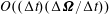 $O((\unicode[STIX]{x0394}t)(\unicode[STIX]{x0394}\unicode[STIX]{x1D734}/\unicode[STIX]{x0394}t))$
contributions that were neglected to obtain (2.7) correspond to
$O((\unicode[STIX]{x0394}t)(\unicode[STIX]{x0394}\unicode[STIX]{x1D734}/\unicode[STIX]{x0394}t))$
contributions that were neglected to obtain (2.7) correspond to
 $O(\unicode[STIX]{x0394}t^{2})$
corrections.
$O(\unicode[STIX]{x0394}t^{2})$
corrections.
Summarizing, provided that
 $\unicode[STIX]{x1D6FF}\ll 1$
(which is always the case), the above reasoning indicates that none of the terms neglected in the derivation of (2.6), (2.7) can be larger than
$\unicode[STIX]{x1D6FF}\ll 1$
(which is always the case), the above reasoning indicates that none of the terms neglected in the derivation of (2.6), (2.7) can be larger than
 $O(\unicode[STIX]{x0394}t^{2})$
whatever
$O(\unicode[STIX]{x0394}t^{2})$
whatever
 $\overline{\unicode[STIX]{x1D70C}}$
. As
$\overline{\unicode[STIX]{x1D70C}}$
. As
 $\boldsymbol{u}^{\prime }$
depends linearly on
$\boldsymbol{u}^{\prime }$
depends linearly on
 $\unicode[STIX]{x0394}\boldsymbol{V}$
and
$\unicode[STIX]{x0394}\boldsymbol{V}$
and
 $\unicode[STIX]{x0394}\unicode[STIX]{x1D734}$
according to (2.3)–(2.5),
$\unicode[STIX]{x0394}\unicode[STIX]{x1D734}$
according to (2.3)–(2.5),
 $\boldsymbol{u}^{\prime }$
is also second-order time accurate.
$\boldsymbol{u}^{\prime }$
is also second-order time accurate.
An interesting outcome of the above analysis is the relative magnitude of the translational and rotational accelerations that the sphere may undergo during a short time interval
 $\unicode[STIX]{x0394}t$
: while
$\unicode[STIX]{x0394}t$
: while
 $\unicode[STIX]{x0394}\boldsymbol{V}/\unicode[STIX]{x0394}t$
may be of
$\unicode[STIX]{x0394}\boldsymbol{V}/\unicode[STIX]{x0394}t$
may be of
 $O(1)$
whatever
$O(1)$
whatever
 $\overline{\unicode[STIX]{x1D70C}}$
thanks to the fluid inertia,
$\overline{\unicode[STIX]{x1D70C}}$
thanks to the fluid inertia,
 $\unicode[STIX]{x0394}\unicode[STIX]{x1D734}/\unicode[STIX]{x0394}t$
is smaller by an
$\unicode[STIX]{x0394}\unicode[STIX]{x1D734}/\unicode[STIX]{x0394}t$
is smaller by an
 $O(\unicode[STIX]{x0394}t)$
factor down to a small value of
$O(\unicode[STIX]{x0394}t)$
factor down to a small value of
 $\overline{\unicode[STIX]{x1D70C}}$
. However for sufficiently small sphere densities, the resistance to the angular acceleration is due to unsteady viscous effects rather than to the sphere rotational inertia, which makes
$\overline{\unicode[STIX]{x1D70C}}$
. However for sufficiently small sphere densities, the resistance to the angular acceleration is due to unsteady viscous effects rather than to the sphere rotational inertia, which makes
 $\unicode[STIX]{x0394}\unicode[STIX]{x1D734}/\unicode[STIX]{x0394}t$
be smaller than
$\unicode[STIX]{x0394}\unicode[STIX]{x1D734}/\unicode[STIX]{x0394}t$
be smaller than
 $\unicode[STIX]{x0394}\boldsymbol{V}/\unicode[STIX]{x0394}t$
only by a factor of
$\unicode[STIX]{x0394}\boldsymbol{V}/\unicode[STIX]{x0394}t$
only by a factor of
 $O(\unicode[STIX]{x0394}t^{1/2})$
. In both regimes, the smaller magnitude of the rotational acceleration compared to its translational counterpart is specific to the sphere geometry, as it results from the fact that the surface pressure does not contribute to the torque.
$O(\unicode[STIX]{x0394}t^{1/2})$
. In both regimes, the smaller magnitude of the rotational acceleration compared to its translational counterpart is specific to the sphere geometry, as it results from the fact that the surface pressure does not contribute to the torque.
Appendix B. Grid characteristics, time step control and preliminary tests
The grid is stretched in the radial (
 $r$
) direction in the following manner: the first four layers of cells surrounding the sphere have a uniform thickness; then the spacing follows a geometric progression with a common ratio
$r$
) direction in the following manner: the first four layers of cells surrounding the sphere have a uniform thickness; then the spacing follows a geometric progression with a common ratio
 $1.075$
up to
$1.075$
up to
 $r=8.5d$
and a second common ratio
$r=8.5d$
and a second common ratio
 $1.15$
in the outer region
$1.15$
in the outer region
 $r>8.5d$
. This radial discretization depends on
$r>8.5d$
. This radial discretization depends on
 $Ar$
. In the highest range of
$Ar$
. In the highest range of
 $Ar$
considered in this study (
$Ar$
considered in this study (
 $400<Ar\leqslant 700$
), the minimum radial spacing,
$400<Ar\leqslant 700$
), the minimum radial spacing,
 $\unicode[STIX]{x0394}r_{m}$
, at the sphere surface is set to
$\unicode[STIX]{x0394}r_{m}$
, at the sphere surface is set to
 $3.3\,10^{-3}d$
, implying a total number of 94 cells in the radial direction. At smaller
$3.3\,10^{-3}d$
, implying a total number of 94 cells in the radial direction. At smaller
 $Ar$
,
$Ar$
,
 $\unicode[STIX]{x0394}r_{m}$
is increased up to
$\unicode[STIX]{x0394}r_{m}$
is increased up to
 $0.01d$
, reducing the number of cells in the radial direction to 86. Thanks to a specific staggered localization of the pressure and velocity components (Magnaudet, Rivero & Fabre Reference Magnaudet, Rivero and Fabre1995; Calmet & Magnaudet Reference Calmet and Magnaudet1997), the present code is known to accurately capture boundary layers with a limited number of cells, typically three to four within the first
$0.01d$
, reducing the number of cells in the radial direction to 86. Thanks to a specific staggered localization of the pressure and velocity components (Magnaudet, Rivero & Fabre Reference Magnaudet, Rivero and Fabre1995; Calmet & Magnaudet Reference Calmet and Magnaudet1997), the present code is known to accurately capture boundary layers with a limited number of cells, typically three to four within the first
 $Re^{-1/2}$
-thick shell surrounding the body (see Magnaudet & Mougin (Reference Magnaudet and Mougin2007) and references therein). We relied on this background to select the above values of
$Re^{-1/2}$
-thick shell surrounding the body (see Magnaudet & Mougin (Reference Magnaudet and Mougin2007) and references therein). We relied on this background to select the above values of
 $\unicode[STIX]{x0394}r_{m}$
which, for the two grids used for
$\unicode[STIX]{x0394}r_{m}$
which, for the two grids used for
 $Ar\leqslant 400$
and
$Ar\leqslant 400$
and
 $Ar>400$
, respectively result in four and six cells within this shell at the highest
$Ar>400$
, respectively result in four and six cells within this shell at the highest
 $Re$
reached in each series. Specific tests performed at various values of
$Re$
reached in each series. Specific tests performed at various values of
 $Ar$
, an example of which is shown in figure 23, confirmed that the above choices yield converged results with respect to
$Ar$
, an example of which is shown in figure 23, confirmed that the above choices yield converged results with respect to
 $\unicode[STIX]{x0394}r_{m}$
whatever
$\unicode[STIX]{x0394}r_{m}$
whatever
 $Ar$
.
$Ar$
.
Figure 23. Influence of the radial grid spacing within the boundary layer on the path of a sphere with
 $Ar=200$
and
$Ar=200$
and
 $\overline{\unicode[STIX]{x1D70C}}=0.5$
(
$\overline{\unicode[STIX]{x1D70C}}=0.5$
(
 $Re_{m}^{-1/2}\approx 0.012$
); red curve:
$Re_{m}^{-1/2}\approx 0.012$
); red curve:
 $\unicode[STIX]{x0394}r_{m}/d=5\times 10^{-3}$
, green curve:
$\unicode[STIX]{x0394}r_{m}/d=5\times 10^{-3}$
, green curve:
 $\unicode[STIX]{x0394}r_{m}/d=7\times 10^{-3}$
, black curve:
$\unicode[STIX]{x0394}r_{m}/d=7\times 10^{-3}$
, black curve:
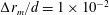 $\unicode[STIX]{x0394}r_{m}/d=1\times 10^{-2}$
; the horizontal (
$\unicode[STIX]{x0394}r_{m}/d=1\times 10^{-2}$
; the horizontal (
 $x$
) and vertical (
$x$
) and vertical (
 $z$
) axes are normalized with the sphere diameter,
$z$
) axes are normalized with the sphere diameter,
 $d$
.
$d$
.
The grid is uniform along the polar (
 $\unicode[STIX]{x1D703}$
) and azimuthal (
$\unicode[STIX]{x1D703}$
) and azimuthal (
 $\unicode[STIX]{x1D719}$
) directions and involves respectively 64 and 128 cells in these directions whatever
$\unicode[STIX]{x1D719}$
) directions and involves respectively 64 and 128 cells in these directions whatever
 $Ar$
. The azimuthal discretization,
$Ar$
. The azimuthal discretization,
 $\unicode[STIX]{x0394}\unicode[STIX]{x1D719}=\unicode[STIX]{x03C0}/64$
, is consistent with that used by Orr et al. (Reference Orr, Domaradzki, Spedding and Constantinescu2015) who considered the flow about a fixed sphere at a Reynolds number of
$\unicode[STIX]{x0394}\unicode[STIX]{x1D719}=\unicode[STIX]{x03C0}/64$
, is consistent with that used by Orr et al. (Reference Orr, Domaradzki, Spedding and Constantinescu2015) who considered the flow about a fixed sphere at a Reynolds number of
 $10^{3}$
and selected
$10^{3}$
and selected
 $\unicode[STIX]{x0394}\unicode[STIX]{x1D719}=\unicode[STIX]{x03C0}/60$
. A twice coarser azimuthal resolution was found to produce identical results for
$\unicode[STIX]{x0394}\unicode[STIX]{x1D719}=\unicode[STIX]{x03C0}/60$
. A twice coarser azimuthal resolution was found to produce identical results for
 $Ar\leqslant 300$
but we kept the above one even in this moderate-
$Ar\leqslant 300$
but we kept the above one even in this moderate-
 $Ar$
range, to make sure that a marginally sufficient resolution could not be the source of potential differences with numerical results available in that range where a succession of dynamical regimes takes place. Specific tests were performed to evaluate the potential effects of the difference in size and shape between cells lying along the
$Ar$
range, to make sure that a marginally sufficient resolution could not be the source of potential differences with numerical results available in that range where a succession of dynamical regimes takes place. Specific tests were performed to evaluate the potential effects of the difference in size and shape between cells lying along the
 $\unicode[STIX]{x1D703}=(0,\unicode[STIX]{x03C0})$
polar axis, which exhibit triangular facets on any spherical surface
$\unicode[STIX]{x1D703}=(0,\unicode[STIX]{x03C0})$
polar axis, which exhibit triangular facets on any spherical surface
 $r=\text{const}.$
and have a small volume, due to the
$r=\text{const}.$
and have a small volume, due to the
 $r^{2}\sin \unicode[STIX]{x1D703}$
Jacobian, and those located about the sphere equator
$r^{2}\sin \unicode[STIX]{x1D703}$
Jacobian, and those located about the sphere equator
 $(\unicode[STIX]{x1D703}=\unicode[STIX]{x03C0}/2)$
which have quadrangular facets and a much larger volume. With 64 cells in in the polar direction, we found that drag (respectively added-mass) coefficients obtained with a sphere translating steadily (respectively unsteadily) along the polar axis differ from those obtained with a sphere crossing this axis at right angle by approximately 0.01 %, a difference which we observed to have negligible effects on the sphere dynamics. Having fixed the number of cells in the azimuthal direction, we kept the polar discretization,
$(\unicode[STIX]{x1D703}=\unicode[STIX]{x03C0}/2)$
which have quadrangular facets and a much larger volume. With 64 cells in in the polar direction, we found that drag (respectively added-mass) coefficients obtained with a sphere translating steadily (respectively unsteadily) along the polar axis differ from those obtained with a sphere crossing this axis at right angle by approximately 0.01 %, a difference which we observed to have negligible effects on the sphere dynamics. Having fixed the number of cells in the azimuthal direction, we kept the polar discretization,
 $\unicode[STIX]{x0394}\unicode[STIX]{x1D703}$
, unchanged whatever
$\unicode[STIX]{x0394}\unicode[STIX]{x1D703}$
, unchanged whatever
 $Ar$
because decreasing it below the minimum (reached at
$Ar$
because decreasing it below the minimum (reached at
 $\unicode[STIX]{x1D703}=\unicode[STIX]{x03C0}/2$
) of the azimuthal discretization,
$\unicode[STIX]{x1D703}=\unicode[STIX]{x03C0}/2$
) of the azimuthal discretization,
 $\sin \unicode[STIX]{x1D703}\unicode[STIX]{x0394}\unicode[STIX]{x1D719}$
, does not increase the overall accuracy, given the arbitrary orientation of the wake with respect to the grid axis. Actually, decreasing
$\sin \unicode[STIX]{x1D703}\unicode[STIX]{x0394}\unicode[STIX]{x1D719}$
, does not increase the overall accuracy, given the arbitrary orientation of the wake with respect to the grid axis. Actually, decreasing
 $\unicode[STIX]{x0394}\unicode[STIX]{x1D703}$
below
$\unicode[STIX]{x0394}\unicode[STIX]{x1D703}$
below
 $\unicode[STIX]{x0394}\unicode[STIX]{x1D719}$
may even be detrimental because it tends to increase the overall grid anisotropy.
$\unicode[STIX]{x0394}\unicode[STIX]{x1D719}$
may even be detrimental because it tends to increase the overall grid anisotropy.
On the outer boundary, the absolute fluid velocity
 $\boldsymbol{U}$
is set to zero everywhere except in the ‘cap’ region intersecting the wake, where the outflow condition described in Magnaudet et al. (Reference Magnaudet, Rivero and Fabre1995) and Auguste (Reference Auguste2010) is used; in short this condition assumes that the first (second) normal derivative of the tangential (normal) velocity component is zero on this cap, together with the second-order cross-derivative of the pressure disturbance. The frontier between the two parts of the outer boundary evolves dynamically as the sphere rotates, according to the sign of the instantaneous normal velocity component (see Auguste et al. (Reference Auguste, Magnaudet and Fabre2013) for details). Auguste (Reference Auguste2010) showed that, compared with standard far-field conditions, this time-evolving treatment drastically reduces the influence of the outer boundary on the predicted dynamics and prevents the development of numerical instabilities, allowing for the use of significantly smaller computational domains. He also established that at least two successive vortices with reduced frequency
$\boldsymbol{U}$
is set to zero everywhere except in the ‘cap’ region intersecting the wake, where the outflow condition described in Magnaudet et al. (Reference Magnaudet, Rivero and Fabre1995) and Auguste (Reference Auguste2010) is used; in short this condition assumes that the first (second) normal derivative of the tangential (normal) velocity component is zero on this cap, together with the second-order cross-derivative of the pressure disturbance. The frontier between the two parts of the outer boundary evolves dynamically as the sphere rotates, according to the sign of the instantaneous normal velocity component (see Auguste et al. (Reference Auguste, Magnaudet and Fabre2013) for details). Auguste (Reference Auguste2010) showed that, compared with standard far-field conditions, this time-evolving treatment drastically reduces the influence of the outer boundary on the predicted dynamics and prevents the development of numerical instabilities, allowing for the use of significantly smaller computational domains. He also established that at least two successive vortices with reduced frequency
 $St$
(i.e. the most intense produced in the wake) have to stand within the computational domain for the outer boundary located at a distance
$St$
(i.e. the most intense produced in the wake) have to stand within the computational domain for the outer boundary located at a distance
 $r_{max}$
from the body centre to generate negligible disturbances within the computational domain when one of them is shed. We confirmed this rule of thumb in the sphere case, based on a series of tests with increasing values of
$r_{max}$
from the body centre to generate negligible disturbances within the computational domain when one of them is shed. We confirmed this rule of thumb in the sphere case, based on a series of tests with increasing values of
 $r_{max}$
. We found
$r_{max}$
. We found
 $r_{max}/d=12$
to work satisfactorily up to
$r_{max}/d=12$
to work satisfactorily up to
 $Ar\approx 300$
but had to gradually increase the domain size with
$Ar\approx 300$
but had to gradually increase the domain size with
 $Ar$
beyond that limit to properly accommodate the less energetic vortices with reduced frequencies smaller than
$Ar$
beyond that limit to properly accommodate the less energetic vortices with reduced frequencies smaller than
 $St$
that develop progressively as
$St$
that develop progressively as
 $Ar$
increases. In the high-
$Ar$
increases. In the high-
 $Ar$
range, these tests provided
$Ar$
range, these tests provided
 $r_{max}$
-independent paths when the outer radius was increased up to
$r_{max}$
-independent paths when the outer radius was increased up to
 $r_{max}/d=17$
, which captures vortices down to an approximate reduced frequency of
$r_{max}/d=17$
, which captures vortices down to an approximate reduced frequency of
 $St/3$
at
$St/3$
at
 $Ar=700$
. This downstream distance is comparable, albeit slightly shorter, than that selected by Poon et al. (Reference Poon, Ooi, Giacobello, Iaccarino and Chung2014) who considered the fixed-sphere case at a Reynolds number of
$Ar=700$
. This downstream distance is comparable, albeit slightly shorter, than that selected by Poon et al. (Reference Poon, Ooi, Giacobello, Iaccarino and Chung2014) who considered the fixed-sphere case at a Reynolds number of
 $10^{3}$
and placed the outlet of their cylindrical domain
$10^{3}$
and placed the outlet of their cylindrical domain
 $20d$
downstream of the sphere centre. We eventually kept the outer radius unchanged at lower
$20d$
downstream of the sphere centre. We eventually kept the outer radius unchanged at lower
 $Ar$
, again to make sure that potential differences with available results could not result from a marginally convenient domain size.
$Ar$
, again to make sure that potential differences with available results could not result from a marginally convenient domain size.
The maximum time step ensuring the stability of the Navier–Stokes solver results from the usual Courant–Friedrichs–Lewy condition, which, given the form of the advective term in (2.2), is based on the components of the relative velocity
 $\boldsymbol{U}-\boldsymbol{V}-\unicode[STIX]{x1D734}\times \boldsymbol{r}$
. However this criterion is not sufficient to guarantee that the time scales inherent to the fluid/body coupling are properly captured. To this end, we impose that any point of the sphere surface cannot move by more than one cell during a time step. Applying this condition to both tangential and normal displacements of the sphere surface indicates that, with the present grid, the minimum time step is dictated by the latter, i.e. by the distance
$\boldsymbol{U}-\boldsymbol{V}-\unicode[STIX]{x1D734}\times \boldsymbol{r}$
. However this criterion is not sufficient to guarantee that the time scales inherent to the fluid/body coupling are properly captured. To this end, we impose that any point of the sphere surface cannot move by more than one cell during a time step. Applying this condition to both tangential and normal displacements of the sphere surface indicates that, with the present grid, the minimum time step is dictated by the latter, i.e. by the distance
 $(\boldsymbol{V}\boldsymbol{\cdot }\boldsymbol{n})\unicode[STIX]{x0394}t$
travelled by the sphere during one time step. The consequences of this condition depend on the orientation of the grid axis with respect to
$(\boldsymbol{V}\boldsymbol{\cdot }\boldsymbol{n})\unicode[STIX]{x0394}t$
travelled by the sphere during one time step. The consequences of this condition depend on the orientation of the grid axis with respect to
 $\boldsymbol{V}$
, since the relevant cell size is
$\boldsymbol{V}$
, since the relevant cell size is
 $\unicode[STIX]{x0394}r_{m}$
when they are aligned, whereas it is dictated by the minimum of
$\unicode[STIX]{x0394}r_{m}$
when they are aligned, whereas it is dictated by the minimum of
 $\sin \unicode[STIX]{x1D703}\unicode[STIX]{x0394}\unicode[STIX]{x1D719}$
when they are at right angle. For this reason, the time step generally evolves during a run according to the variations of this relative orientation. Applying the above criterion then yields
$\sin \unicode[STIX]{x1D703}\unicode[STIX]{x0394}\unicode[STIX]{x1D719}$
when they are at right angle. For this reason, the time step generally evolves during a run according to the variations of this relative orientation. Applying the above criterion then yields
 $\unicode[STIX]{x1D708}\unicode[STIX]{x0394}t/d^{2}=k\unicode[STIX]{x1D6FC}(t)Ar^{-1}$
, where
$\unicode[STIX]{x1D708}\unicode[STIX]{x0394}t/d^{2}=k\unicode[STIX]{x1D6FC}(t)Ar^{-1}$
, where
 $k=((1-\overline{\unicode[STIX]{x1D70C}})gd)^{1/2}/\Vert \boldsymbol{V}\Vert$
stands in the range 0.6–0.7 according to the
$k=((1-\overline{\unicode[STIX]{x1D70C}})gd)^{1/2}/\Vert \boldsymbol{V}\Vert$
stands in the range 0.6–0.7 according to the
 $Ar-Re$
relationship (see figure 20
a), and
$Ar-Re$
relationship (see figure 20
a), and
 $\unicode[STIX]{x1D6FC}(t)$
may vary over time from
$\unicode[STIX]{x1D6FC}(t)$
may vary over time from
 $\unicode[STIX]{x0394}r_{m}/d$
to
$\unicode[STIX]{x0394}r_{m}/d$
to
 $(\unicode[STIX]{x03C0}/128)^{2}$
for the above reason. Hence, within a run, the dimensionless time step may vary from
$(\unicode[STIX]{x03C0}/128)^{2}$
for the above reason. Hence, within a run, the dimensionless time step may vary from
 $4\times 10^{-4}Ar^{-1}$
to
$4\times 10^{-4}Ar^{-1}$
to
 $7\times 10^{-3}Ar^{-1}$
. Various tests were performed to compare results obtained by imposing a fixed time step with those based on this criterion. They allowed us to conclude that the latter yields
$7\times 10^{-3}Ar^{-1}$
. Various tests were performed to compare results obtained by imposing a fixed time step with those based on this criterion. They allowed us to conclude that the latter yields
 $\unicode[STIX]{x0394}t$
-independent predictions in the various regimes of rise.
$\unicode[STIX]{x0394}t$
-independent predictions in the various regimes of rise.
Table 1. Several global and near-wake statistical characteristics of the flow past a fixed sphere at
 $Re=10^{3}$
. The drag and lift coefficients,
$Re=10^{3}$
. The drag and lift coefficients,
 $C_{D}$
and
$C_{D}$
and
 $C_{L}$
, are defined as the corresponding time-averaged component of the force on the sphere divided by
$C_{L}$
, are defined as the corresponding time-averaged component of the force on the sphere divided by
 $\unicode[STIX]{x03C0}/8$
(
$\unicode[STIX]{x03C0}/8$
(
 $\unicode[STIX]{x1D70C}=1$
,
$\unicode[STIX]{x1D70C}=1$
,
 $d=1$
,
$d=1$
,
 $U=1$
at infinity);
$U=1$
at infinity);
 $U$
and
$U$
and
 $u^{\prime }$
are respectively the mean and root-mean-square streamwise velocities on the wake axis,
$u^{\prime }$
are respectively the mean and root-mean-square streamwise velocities on the wake axis,
 $U_{min}$
is the (negative) minimum of
$U_{min}$
is the (negative) minimum of
 $U$
, reached at the streamwise position
$U$
, reached at the streamwise position
 $x_{U_{min}}$
within the recirculation bubble (with
$x_{U_{min}}$
within the recirculation bubble (with
 $x=0$
at the sphere centre),
$x=0$
at the sphere centre),
 $x_{U=0}$
is the time-averaged position of the tail of the recirculation bubble (i.e. the averaged ‘standing eddy length’),
$x_{U=0}$
is the time-averaged position of the tail of the recirculation bubble (i.e. the averaged ‘standing eddy length’),
 $x_{U=0.9}$
is the streamwise position at which
$x_{U=0.9}$
is the streamwise position at which
 $U$
has recovered 90 % of its upstream value, and
$U$
has recovered 90 % of its upstream value, and
 $x_{u_{max}^{\prime }}$
the one at which
$x_{u_{max}^{\prime }}$
the one at which
 $u^{\prime }$
reaches its maximum,
$u^{\prime }$
reaches its maximum,
 $u_{max}^{\prime }$
.
$u_{max}^{\prime }$
.
The boundary-fitted version of the JADIM code was extensively used over the last two decades to compute flows past various axisymmetric bodies at moderate Reynolds numbers, most often below
 $500$
. In Magnaudet & Mougin (Reference Magnaudet and Mougin2007), characteristics of the first two transitional states of the flow past a fixed sphere were computed at Reynolds numbers of 250 and 300 on a grid similar to the one described above, albeit with a twice coarser azimuthal resolution. Results were compared with available data, especially those of Johnson & Patel (Reference Johnson and Patel1999). A very good agreement was noticed in both states, especially on the drag and lift coefficients (including their root-mean-square at
$500$
. In Magnaudet & Mougin (Reference Magnaudet and Mougin2007), characteristics of the first two transitional states of the flow past a fixed sphere were computed at Reynolds numbers of 250 and 300 on a grid similar to the one described above, albeit with a twice coarser azimuthal resolution. Results were compared with available data, especially those of Johnson & Patel (Reference Johnson and Patel1999). A very good agreement was noticed in both states, especially on the drag and lift coefficients (including their root-mean-square at
 $Re=300$
). At the beginning of the present study, a series of simulations with fixed spheres was run in the range
$Re=300$
). At the beginning of the present study, a series of simulations with fixed spheres was run in the range
 $200\leqslant Re\leqslant 400$
with the standard grid described above. At
$200\leqslant Re\leqslant 400$
with the standard grid described above. At
 $Re=300$
, the Strouhal number was found to be
$Re=300$
, the Strouhal number was found to be
 $St=0.136$
, in perfect agreement with the predictions of Johnson & Patel (Reference Johnson and Patel1999) and Tomboulides & Orszag (Reference Tomboulides and Orszag2000). Transition to three-dimensional flow in the wake was observed to take place at
$St=0.136$
, in perfect agreement with the predictions of Johnson & Patel (Reference Johnson and Patel1999) and Tomboulides & Orszag (Reference Tomboulides and Orszag2000). Transition to three-dimensional flow in the wake was observed to take place at
 $Re\approx 370$
, which stands within the interval
$Re\approx 370$
, which stands within the interval
 $350<Re<375$
where it was first identified by Mittal (Reference Mittal1999).
$350<Re<375$
where it was first identified by Mittal (Reference Mittal1999).
Regarding the fluid/body couplings that play a crucial role in the present problem, the basic version of the algorithm detailed in § 2.2 (i.e. without the
 $\unicode[STIX]{x1D6FF}$
-terms in (2.6), (2.7) and the viscous
$\unicode[STIX]{x1D6FF}$
-terms in (2.6), (2.7) and the viscous
 $\boldsymbol{u}^{\unicode[STIX]{x1D6FF}}$
contribution to the velocity correction
$\boldsymbol{u}^{\unicode[STIX]{x1D6FF}}$
contribution to the velocity correction
 $\boldsymbol{u}^{\prime }$
), was successfully employed to determine the nature and thresholds of the first transitions to the fluttering and tumbling regimes of disks and cylinders with various aspect ratios (Auguste Reference Auguste2010; Auguste et al.
Reference Auguste, Magnaudet and Fabre2013). Somewhat later, results were published independently on the same problem by Chrust et al. (Reference Chrust, Bouchet and Dušek2013, Reference Chrust, Bouchet and Dušek2014). The two series of results were found to be in very close agreement (see § 5.2 for more details).
$\boldsymbol{u}^{\prime }$
), was successfully employed to determine the nature and thresholds of the first transitions to the fluttering and tumbling regimes of disks and cylinders with various aspect ratios (Auguste Reference Auguste2010; Auguste et al.
Reference Auguste, Magnaudet and Fabre2013). Somewhat later, results were published independently on the same problem by Chrust et al. (Reference Chrust, Bouchet and Dušek2013, Reference Chrust, Bouchet and Dušek2014). The two series of results were found to be in very close agreement (see § 5.2 for more details).
This background of the JADIM code, combined with the supplementary tests performed in the range
 $200\leqslant Re\leqslant 400$
with fixed spheres and the improvements of the fluid/body coupling algorithm described in § 2.2, establish that, with the grid characteristics discussed above, this code can reliably deal with path instabilities of light rising spheres up to Reynolds numbers of several hundred. Nevertheless it was still necessary to prove that accurate results may be obtained on the grid with
$200\leqslant Re\leqslant 400$
with fixed spheres and the improvements of the fluid/body coupling algorithm described in § 2.2, establish that, with the grid characteristics discussed above, this code can reliably deal with path instabilities of light rising spheres up to Reynolds numbers of several hundred. Nevertheless it was still necessary to prove that accurate results may be obtained on the grid with
 $\unicode[STIX]{x0394}r_{m}/d=3.3\times 10^{-3}$
at significantly larger Reynolds numbers, since we intended to compare them with the experimental observations reported by Veldhuis et al. (Reference Veldhuis, Biesheuvel and Lohse2009) for
$\unicode[STIX]{x0394}r_{m}/d=3.3\times 10^{-3}$
at significantly larger Reynolds numbers, since we intended to compare them with the experimental observations reported by Veldhuis et al. (Reference Veldhuis, Biesheuvel and Lohse2009) for
 $Re\gtrsim 800$
. To this end, considering that the fluid/coupling algorithm had already been fully validated, we performed specific tests in the fixed-sphere case at a Reynolds number
$Re\gtrsim 800$
. To this end, considering that the fluid/coupling algorithm had already been fully validated, we performed specific tests in the fixed-sphere case at a Reynolds number
 $Re=10^{3}$
, for which recent computational data are available (Poon et al.
Reference Poon, Ooi, Giacobello, Iaccarino and Chung2014; Orr et al.
Reference Orr, Domaradzki, Spedding and Constantinescu2015). Some global and near-wake statistical characteristics of the corresponding flow are presented in table 1. Comparison with available data indicates a very good agreement. Time spectra of the drag force and of the near-wake streamwise velocity fluctuation were also found to compare satisfactorily with those reported by Orr et al. (Reference Orr, Domaradzki, Spedding and Constantinescu2015). This test confirms that, with the present grid, our code provides reliable predictions for Reynolds numbers of
$Re=10^{3}$
, for which recent computational data are available (Poon et al.
Reference Poon, Ooi, Giacobello, Iaccarino and Chung2014; Orr et al.
Reference Orr, Domaradzki, Spedding and Constantinescu2015). Some global and near-wake statistical characteristics of the corresponding flow are presented in table 1. Comparison with available data indicates a very good agreement. Time spectra of the drag force and of the near-wake streamwise velocity fluctuation were also found to compare satisfactorily with those reported by Orr et al. (Reference Orr, Domaradzki, Spedding and Constantinescu2015). This test confirms that, with the present grid, our code provides reliable predictions for Reynolds numbers of
 $O(10^{3})$
, despite the quite short distance at which the outer boundary intersects the wake and the limited number of cells that still stand within the latter when the streamwise distance increases (only 6–8 cells lie in the wake in the polar direction at
$O(10^{3})$
, despite the quite short distance at which the outer boundary intersects the wake and the limited number of cells that still stand within the latter when the streamwise distance increases (only 6–8 cells lie in the wake in the polar direction at
 $x/d=10$
, owing to the choice
$x/d=10$
, owing to the choice
 $\unicode[STIX]{x0394}\unicode[STIX]{x1D703}=\unicode[STIX]{x03C0}/64$
).
$\unicode[STIX]{x0394}\unicode[STIX]{x1D703}=\unicode[STIX]{x03C0}/64$
).