


1 Introduction
Modern studies on the impact of projectiles in water started with the experimental work of Worthington and Cole (Worthington & Cole Reference Worthington and Cole1900). The question is broad and has drawn the attention of many researchers (Birkhoff & Zarantonello Reference Birkhoff and Zarantonello1957; Truscott, Epps & Belden Reference Truscott, Epps and Belden2014) as it covers subjects as diverse as explaining how animals can walk on water (Glasheen & McMahon Reference Glasheen and McMahon1996a ,Reference Glasheen and McMahon b ; Bergmann et al. Reference Bergmann, Van Der Meer, Gekle, Van Der Bos and Lohse2009), understanding the dive of birds like gannets (Adams & Walter Reference Adams and Walter1993; Prince, Huin & Weimerskirch Reference Prince, Huin and Weimerskirch1994; Brierley & Fernandes Reference Brierley and Fernandes2001; Chang et al. Reference Chang, Croson, Straker, Gart, Dove, Gerwin and Jung2016), quantifying the ability of a liquid to absorb energy or designing the shape of missiles (May Reference May1952, Reference May1975; Lee, Longoria & Wilson Reference Lee, Longoria and Wilson1997) and floats (Von Karman Reference Von Karman1929). Early works were devoted to the description of the projectile entry and to the formation of air cavities (Gilbarg & Anderson Reference Gilbarg and Anderson1948; May Reference May1952, Reference May1975; Gaudet Reference Gaudet1998; Duclaux et al. Reference Duclaux, Caillé, Duez, Ybert, Bocquet and Clanet2007; Aristoff & Bush Reference Aristoff and Bush2009), which, when asymmetric, can deviate the projectile underwater (Bodily, Carlson & Truscott Reference Bodily, Carlson and Truscott2014). More generally, it was shown than trajectories after the pinch-off of the cavity (Gekle & Gordillo Reference Gekle and Gordillo2010) can be non-straight (Mansoor et al. Reference Mansoor, Vakarelski, Marston, Truscott and Thoroddsen2017; Vakarelski et al. Reference Vakarelski, Klaseboer, Jetly, Mansoor, Aguirre-Pablo, Chan and Thoroddsen2017), even in an infinite bath (Ern et al. Reference Ern, Risso, Fabre and Magnaudet2012) – following for instance oscillating or curved paths (Willmarth, Hawk & Harvey Reference Willmarth, Hawk and Harvey1964; Mahadevan Reference Mahadevan1996; Fernandes et al. Reference Fernandes, Risso, Ern and Magnaudet2007; Auguste, Fabre & Magnaudet Reference Auguste, Fabre and Magnaudet2010).
In this article, we focus on the trajectory of floating axisymmetric streamlined bodies penetrating a bath of water, either vertically or with an angle toward the vertical. After describing our set-up (§ 2), we present the experimental results in § 3 and model them in § 4, the final § 5 being devoted to scaling laws and numerical solutions.
2 Experimental details
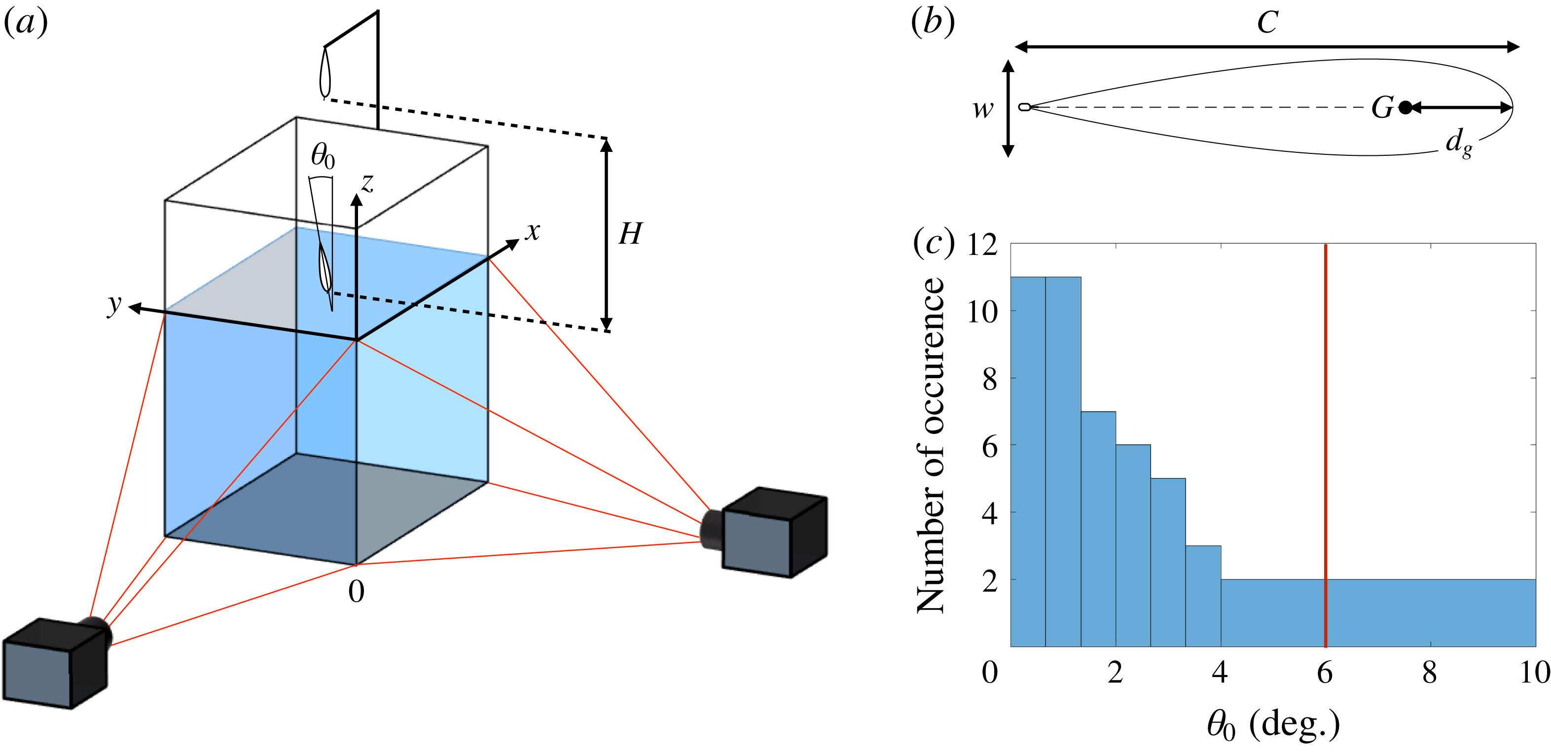
Figure 1. (a) Sketch of the set-up used to follow the underwater trajectory of the projectiles;
 $\unicode[STIX]{x1D703}_{0}$
is the angle between the axis of symmetry of the projectile and the vertical at the impact. The projectile is released at a height
$\unicode[STIX]{x1D703}_{0}$
is the angle between the axis of symmetry of the projectile and the vertical at the impact. The projectile is released at a height
 $H$
above the water surface. (b) Sectional drawing of the projectiles used for our experiments. The dashed line represents the chord and is used as the rotation axis to create the three-dimensional axisymmetric projectile where the centre of gravity
$H$
above the water surface. (b) Sectional drawing of the projectiles used for our experiments. The dashed line represents the chord and is used as the rotation axis to create the three-dimensional axisymmetric projectile where the centre of gravity
 $G$
is located at a distance
$G$
is located at a distance
 $d_{g}$
from the leading edge. The projectile has a length
$d_{g}$
from the leading edge. The projectile has a length
 $C$
and a maximum width
$C$
and a maximum width
 $w$
and its aspect ratio
$w$
and its aspect ratio
 $\unicode[STIX]{x1D712}=C/w$
is 5 for all our experiments. The eye of a needle is attached to the trailing edge of the projectile. (c) Distribution of the impact angle
$\unicode[STIX]{x1D712}=C/w$
is 5 for all our experiments. The eye of a needle is attached to the trailing edge of the projectile. (c) Distribution of the impact angle
 $\unicode[STIX]{x1D703}_{0}$
for various impact velocities. As marked with the red line, the impact angle is lower than
$\unicode[STIX]{x1D703}_{0}$
for various impact velocities. As marked with the red line, the impact angle is lower than
 $6^{\circ }$
for
$6^{\circ }$
for
 $95\,\%$
of the experiments.
$95\,\%$
of the experiments.
2.1 Trajectory reconstruction
As shown in figure 1(a), our projectiles are released without initial velocity from a height
 $H$
above a square-based tank of dimensions 60 cm by 60 cm by 100 cm. When a projectile reaches the water surface, its impact velocity is
$H$
above a square-based tank of dimensions 60 cm by 60 cm by 100 cm. When a projectile reaches the water surface, its impact velocity is
 $U_{0}$
and its impact angle with the vertical is
$U_{0}$
and its impact angle with the vertical is
 $\unicode[STIX]{x1D703}_{0}$
. Its trajectory is followed using two perpendicular, synchronized cameras recording the motion underwater, as sketched in figure 1(a). We use two high-speed cameras, Photron mini UX-100, equipped with 20mm f/1.8 Nikon lenses, recording at frame rates ranging from 250 to 1500 frames per second. Taking into account magnification due to the passage through the air–water interface as well as the divergence of the field of view of the camera, we determine the three-dimensional position of the centre of gravity of the projectile for each pair of frames recorded by the two cameras with a precision of the order of a few millimetres.
$\unicode[STIX]{x1D703}_{0}$
. Its trajectory is followed using two perpendicular, synchronized cameras recording the motion underwater, as sketched in figure 1(a). We use two high-speed cameras, Photron mini UX-100, equipped with 20mm f/1.8 Nikon lenses, recording at frame rates ranging from 250 to 1500 frames per second. Taking into account magnification due to the passage through the air–water interface as well as the divergence of the field of view of the camera, we determine the three-dimensional position of the centre of gravity of the projectile for each pair of frames recorded by the two cameras with a precision of the order of a few millimetres.
 $U_{0}$
is determined using the first 20 frames following the impact.
$U_{0}$
is determined using the first 20 frames following the impact.
2.2 Projectiles
The projectiles used in our experiments are axisymmetric bodies generated by the rotation of a wing profile around its chord, as shown in figure 1(b). The profile is such that its maximum width
 $w$
is one fifth of the length
$w$
is one fifth of the length
 $C$
of its chord, as defined by the National Advisory Committee for Aeronautics as the profile NACA 0020. The projectiles are 3D printed in acrylonitrile butadiene styrene (ABS) and smoothed above an acetone bath at
$C$
of its chord, as defined by the National Advisory Committee for Aeronautics as the profile NACA 0020. The projectiles are 3D printed in acrylonitrile butadiene styrene (ABS) and smoothed above an acetone bath at
 $70\,^{\circ }\text{C}$
for two minutes. The resulting objects are then coated with Rain-X to increase their hydrophilicity and thus reduce the generation of air cavities when crossing the air–water interface (Duez et al.
Reference Duez, Ybert, Clanet and Bocquet2007). Projectiles are hollowed out and a moving brass cylinder ballasts the body and allows us to tune the position of their centre of gravity. The eye of a needle is attached to their trailing edge for their release.
$70\,^{\circ }\text{C}$
for two minutes. The resulting objects are then coated with Rain-X to increase their hydrophilicity and thus reduce the generation of air cavities when crossing the air–water interface (Duez et al.
Reference Duez, Ybert, Clanet and Bocquet2007). Projectiles are hollowed out and a moving brass cylinder ballasts the body and allows us to tune the position of their centre of gravity. The eye of a needle is attached to their trailing edge for their release.
The projectiles are 75 mm long and 15 mm thick, with an aspect ratio
 $\unicode[STIX]{x1D712}=C/w$
of
$\unicode[STIX]{x1D712}=C/w$
of
 $5$
. Their mass is between
$5$
. Their mass is between
 $6.2$
g and
$6.2$
g and
 $6.9$
g. As they are slender, their added mass is neglected in the rest of the study. Their relative density
$6.9$
g. As they are slender, their added mass is neglected in the rest of the study. Their relative density
 $\bar{\unicode[STIX]{x1D70C}}=\unicode[STIX]{x1D70C}_{projectile}/\unicode[STIX]{x1D70C}_{water}$
ranges from 0.85 to 0.95. The distance
$\bar{\unicode[STIX]{x1D70C}}=\unicode[STIX]{x1D70C}_{projectile}/\unicode[STIX]{x1D70C}_{water}$
ranges from 0.85 to 0.95. The distance
 $d_{g}$
from the leading edge to the centre of mass of the projectile is varied from 18 to 45 % of the cord.
$d_{g}$
from the leading edge to the centre of mass of the projectile is varied from 18 to 45 % of the cord.
2.3 Releasing method
In order to release the projectile without an initial velocity or initial angle, we hold it by the eye of a needle placed at its trailing edge with a
 $105~\unicode[STIX]{x03BC}\text{m}$
-thick nylon fibre attached to 0.5 mm-thick copper wire. Upon a current running through the wire, the nylon melts and the projectile is released vertically. The impact velocity
$105~\unicode[STIX]{x03BC}\text{m}$
-thick nylon fibre attached to 0.5 mm-thick copper wire. Upon a current running through the wire, the nylon melts and the projectile is released vertically. The impact velocity
 $U_{0}$
ranges from 0.1 to
$U_{0}$
ranges from 0.1 to
 $2.1~\text{m}~\text{s}^{-1}$
. The impact angle
$2.1~\text{m}~\text{s}^{-1}$
. The impact angle
 $\unicode[STIX]{x1D703}_{0}$
is measured using two cameras set just above the water’s surface. The histogram in figure 1(c) shows that our method ensures an impact angle below
$\unicode[STIX]{x1D703}_{0}$
is measured using two cameras set just above the water’s surface. The histogram in figure 1(c) shows that our method ensures an impact angle below
 $6^{\circ }$
in
$6^{\circ }$
in
 $95\,\%$
of the experiments.
$95\,\%$
of the experiments.
3 Experimental results
3.1 Nature of the trajectory
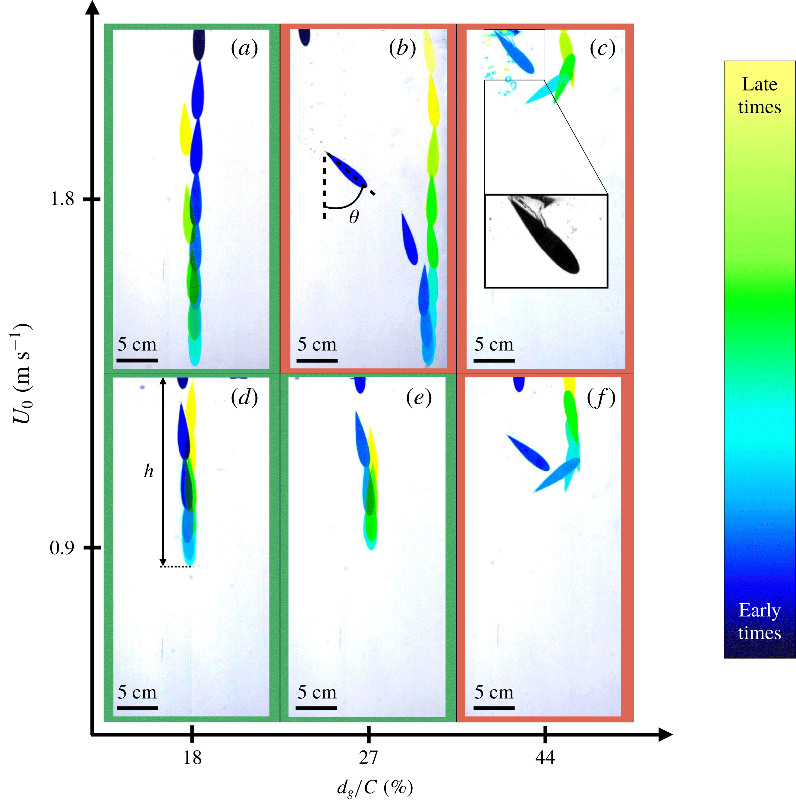
Figure 2. Chronophotographs of the projectile trajectories for various impact velocities
 $U_{0}$
, and for various distances
$U_{0}$
, and for various distances
 $d_{g}$
between the centre of gravity of the projectile and its leading edge. The centre of buoyancy is located at
$d_{g}$
between the centre of gravity of the projectile and its leading edge. The centre of buoyancy is located at
 $37.5\,\%$
of the total chord from the leading edge. For all chronophotographs, frames are separated by 0.15 s. The stable trajectories are boxed in green (a,d,e) whereas the unstable ones are boxed in red (b,c,f).
$37.5\,\%$
of the total chord from the leading edge. For all chronophotographs, frames are separated by 0.15 s. The stable trajectories are boxed in green (a,d,e) whereas the unstable ones are boxed in red (b,c,f).
We display in figure 2 the different possible trajectories of the projectiles, depending on their impact velocity
 $U_{0}$
and location
$U_{0}$
and location
 $d_{g}$
of the centre of mass. In the six presented experiments, projectiles are floating and the global motion is the same: the projectile impacts the water almost vertically, slows down until it reaches its maximum depth before moving back toward the water’s surface.
$d_{g}$
of the centre of mass. In the six presented experiments, projectiles are floating and the global motion is the same: the projectile impacts the water almost vertically, slows down until it reaches its maximum depth before moving back toward the water’s surface.
The two chronophotographs on the left-hand side of figure 2 (panels a,d) correspond to the trajectories of projectiles whose centres of mass are located close to the leading edge (
 $d_{g}/C=18\,\%$
). For such projectiles, both at low impact velocity (
$d_{g}/C=18\,\%$
). For such projectiles, both at low impact velocity (
 $U_{0}\approx 0.9~\text{m}~\text{s}^{-1}$
for 2
d) and high impact velocity (
$U_{0}\approx 0.9~\text{m}~\text{s}^{-1}$
for 2
d) and high impact velocity (
 $U_{0}\approx 1.8~\text{m}~\text{s}^{-1}$
for 2
a), the path followed in the descending phase is a vertical straight line. At the maximum depth of the dive, the projectile has no velocity. Later, it follows the same straight path as in its ascending phase until the trailing edge reaches the water’s surface close to the impact point. The depth
$U_{0}\approx 1.8~\text{m}~\text{s}^{-1}$
for 2
a), the path followed in the descending phase is a vertical straight line. At the maximum depth of the dive, the projectile has no velocity. Later, it follows the same straight path as in its ascending phase until the trailing edge reaches the water’s surface close to the impact point. The depth
 $h$
increases with the impact velocity.
$h$
increases with the impact velocity.
The two chronophotographs centred in figure 2 (panels b,e) correspond to the impacts of a projectile with a centre of mass located at
 $d_{g}/C=27\,\%$
. At low impact velocity (
$d_{g}/C=27\,\%$
. At low impact velocity (
 $U_{0}\approx 0.9~\text{m}~\text{s}^{-1}$
for 2
e), the trajectory followed by the projectile is a vertical straight line in both descending and ascending phases, as observed earlier. However, the trajectory changes at higher impact velocity (
$U_{0}\approx 0.9~\text{m}~\text{s}^{-1}$
for 2
e), the trajectory followed by the projectile is a vertical straight line in both descending and ascending phases, as observed earlier. However, the trajectory changes at higher impact velocity (
 $U_{0}\approx 1.8~\text{m}~\text{s}^{-1}$
for 2
b). In the first half of the descending phase, the projectile rotates such that the angle
$U_{0}\approx 1.8~\text{m}~\text{s}^{-1}$
for 2
b). In the first half of the descending phase, the projectile rotates such that the angle
 $\unicode[STIX]{x1D703}$
between its chord and the vertical increases and its path deviates from a straight line. In the second half of the descending phase, the projectile slowly realigns with the vertical (
$\unicode[STIX]{x1D703}$
between its chord and the vertical increases and its path deviates from a straight line. In the second half of the descending phase, the projectile slowly realigns with the vertical (
 $\unicode[STIX]{x1D703}$
decreases) until it reaches is maximum depth. At this point, the projectile has no velocity and is fully aligned with the vertical with its leading edge pointing down (
$\unicode[STIX]{x1D703}$
decreases) until it reaches is maximum depth. At this point, the projectile has no velocity and is fully aligned with the vertical with its leading edge pointing down (
 $\unicode[STIX]{x1D703}=0$
). Then, in the ascending phase, the projectile follows a vertical straight line up to the water’s surface, which it reaches at a point different from that at impact. We call such a trajectory ‘y-shaped’. Increasing the impact velocity increases the horizontal distance between the entry and exit points.
$\unicode[STIX]{x1D703}=0$
). Then, in the ascending phase, the projectile follows a vertical straight line up to the water’s surface, which it reaches at a point different from that at impact. We call such a trajectory ‘y-shaped’. Increasing the impact velocity increases the horizontal distance between the entry and exit points.
The two chronophotographs on the right-hand side of figure 2 (panels c,f) finally correspond to impacts of a projectile whose centre of mass is located far from the leading edge (
 $d_{g}/C=44\,\%$
). At low impact velocity (
$d_{g}/C=44\,\%$
). At low impact velocity (
 $U_{0}\approx 0.9~\text{m}~\text{s}^{-1}$
for 2
f), the projectile rotates (
$U_{0}\approx 0.9~\text{m}~\text{s}^{-1}$
for 2
f), the projectile rotates (
 $\unicode[STIX]{x1D703}$
continually increases) and the trajectory deviates from the vertical during the descending phase. The projectile reaches its maximum depth horizontally (
$\unicode[STIX]{x1D703}$
continually increases) and the trajectory deviates from the vertical during the descending phase. The projectile reaches its maximum depth horizontally (
 $\unicode[STIX]{x1D703}=90^{\circ }$
) with a non-zero horizontal velocity. In the ascending phase, the projectile keeps on rotating until its leading edge reaches the water surface (
$\unicode[STIX]{x1D703}=90^{\circ }$
) with a non-zero horizontal velocity. In the ascending phase, the projectile keeps on rotating until its leading edge reaches the water surface (
 $\unicode[STIX]{x1D703}\approx 180^{\circ }$
) at a different location from the impact point. Such a trajectory has a ‘U-shape’. Compared with the straight trajectories observed at the same impact velocity for projectiles with centre of mass closer to the leading edge, the projectile travels further horizontally but the dive is shallower. Even though the shape of the trajectory is not modified at higher impact velocity (
$\unicode[STIX]{x1D703}\approx 180^{\circ }$
) at a different location from the impact point. Such a trajectory has a ‘U-shape’. Compared with the straight trajectories observed at the same impact velocity for projectiles with centre of mass closer to the leading edge, the projectile travels further horizontally but the dive is shallower. Even though the shape of the trajectory is not modified at higher impact velocity (
 $U_{0}\approx 1.8~\text{m}~\text{s}^{-1}$
), the depth of the dive is reduced – due to the existence of a large cavity of air entrained at water entry, as shown in the inset of figure 2(c).
$U_{0}\approx 1.8~\text{m}~\text{s}^{-1}$
), the depth of the dive is reduced – due to the existence of a large cavity of air entrained at water entry, as shown in the inset of figure 2(c).
To summarize our observations, three different types of trajectory can be observed: straight, y-shaped and U-shaped. Straight trajectories appear for a centre of mass located close to the leading edge and at low impact velocity. When the velocity is increased, the motion follows a y-shape. Finally, when the centre of mass is far from the leading edge, the trajectory has a U-shape at all velocities.
3.2 Quasi-planar trajectories
For a y-shaped path, a typical three-dimensional (3-D) trajectory of the centre of mass of the projectile is presented in figure 3(a). The projectile impacts water at the coordinates
 $(x_{0},y_{0},0)$
. When plotted in the (O
$(x_{0},y_{0},0)$
. When plotted in the (O
 $xy$
) plane, orthogonal to gravity, the trajectory is close to be planar, apart from the ascending phase, where the projectile slowly drifts and oscillates, as shown in figure 3(b). Hence, we can define the mean vertical plane of the descending phase of the trajectory drawn in yellow in figure 3(b). Finally, we define a new coordinate system
$xy$
) plane, orthogonal to gravity, the trajectory is close to be planar, apart from the ascending phase, where the projectile slowly drifts and oscillates, as shown in figure 3(b). Hence, we can define the mean vertical plane of the descending phase of the trajectory drawn in yellow in figure 3(b). Finally, we define a new coordinate system
 $(\widetilde{x},z)$
centred at the impact point (
$(\widetilde{x},z)$
centred at the impact point (
 $\widetilde{x}=|x-x_{0}|$
) and the 3-D trajectory is projected along the mean plane to obtain the typical 2-D y-shaped trajectory plotted in figure 3(c). This protocol is followed for the three types of trajectory observed (straight, U-shaped, y-shaped).
$\widetilde{x}=|x-x_{0}|$
) and the 3-D trajectory is projected along the mean plane to obtain the typical 2-D y-shaped trajectory plotted in figure 3(c). This protocol is followed for the three types of trajectory observed (straight, U-shaped, y-shaped).

Figure 3. (a) Underwater 3-D trajectory of the centre of mass of the projectile after its impact at the red spot at coordinates
 $(x_{0},y_{0},0)$
. The maximum depth of the dive is reached at the red square. The trajectory is obtained from the images of the two high-speed cameras. (b) The blue curve is the actual trajectory of the projectile projected onto the (O
$(x_{0},y_{0},0)$
. The maximum depth of the dive is reached at the red square. The trajectory is obtained from the images of the two high-speed cameras. (b) The blue curve is the actual trajectory of the projectile projected onto the (O
 $xy$
) plane. Projectile impacts water at the red spot and reaches its maximum depth at the red square. The yellow straight line is the projection of the mean plane of the trajectory in the descending phase onto the (O
$xy$
) plane. Projectile impacts water at the red spot and reaches its maximum depth at the red square. The yellow straight line is the projection of the mean plane of the trajectory in the descending phase onto the (O
 $xy$
) plane. The direction of the axis
$xy$
) plane. The direction of the axis
 $\widetilde{x}$
is contained in the mean plane of the trajectory. (c) Projected trajectory on the mean plane defined in (b). The coordinate
$\widetilde{x}$
is contained in the mean plane of the trajectory. (c) Projected trajectory on the mean plane defined in (b). The coordinate
 $\widetilde{x}=|x-x_{0}|$
is defined such that the origin coincides with the impact point marked by the red spot.
$\widetilde{x}=|x-x_{0}|$
is defined such that the origin coincides with the impact point marked by the red spot.
Figure 4 shows experimental trajectories obtained by varying independently the impact velocity
 $U_{0}$
and the position
$U_{0}$
and the position
 $d_{g}$
of the centre of gravity of the projectile. In figure 4(a), the centre of mass of the projectile is fixed (
$d_{g}$
of the centre of gravity of the projectile. In figure 4(a), the centre of mass of the projectile is fixed (
 $d_{g}/C=35\,\%$
) and the impact velocity is varied. The transition between straight and y-shaped trajectory is observed between
$d_{g}/C=35\,\%$
) and the impact velocity is varied. The transition between straight and y-shaped trajectory is observed between
 $0.23$
and
$0.23$
and
 $0.39~\text{m}~\text{s}^{-1}$
. Above the latter speed, the horizontally travelled distance increases with the impact speed while the maximum depth
$0.39~\text{m}~\text{s}^{-1}$
. Above the latter speed, the horizontally travelled distance increases with the impact speed while the maximum depth
 $h$
hardly depends on
$h$
hardly depends on
 $U_{0}$
.
$U_{0}$
.
As shown in figure 4(b), an increase of the distance
 $d_{g}$
modifies the shape of the trajectory: at
$d_{g}$
modifies the shape of the trajectory: at
 $U_{0}=0.91~\text{m}~\text{s}^{-1}$
when
$U_{0}=0.91~\text{m}~\text{s}^{-1}$
when
 $d_{g}/C<33\,\%$
, the trajectory is straight, when
$d_{g}/C<33\,\%$
, the trajectory is straight, when
 $33\,\%\leqslant d_{g}/C<38\,\%$
, the trajectory has a y-shape and above
$33\,\%\leqslant d_{g}/C<38\,\%$
, the trajectory has a y-shape and above
 $38\,\%$
, the trajectory is U-shaped. Overall, when
$38\,\%$
, the trajectory is U-shaped. Overall, when
 $d_{g}$
is increased at fixed impact velocity, the depth of the dive is reduced and the horizontal distance travelled is increased. Hence, there is an optimal impact velocity and position of the centre of mass such that the dive depth
$d_{g}$
is increased at fixed impact velocity, the depth of the dive is reduced and the horizontal distance travelled is increased. Hence, there is an optimal impact velocity and position of the centre of mass such that the dive depth
 $h$
is maximum.
$h$
is maximum.

Figure 4. (a) Experimental trajectories for a projectile with a fixed position of the centre of gravity (
 $d_{g}/C=35\,\%$
) and a mass of
$d_{g}/C=35\,\%$
) and a mass of
 $m=6.4~\text{g}$
. The impact velocity
$m=6.4~\text{g}$
. The impact velocity
 $U_{0}$
is varied from 0.23 to
$U_{0}$
is varied from 0.23 to
 $1.46~\text{m}~\text{s}^{-1}$
. Red crosses represent the maximum depth of the dive
$1.46~\text{m}~\text{s}^{-1}$
. Red crosses represent the maximum depth of the dive
 $h$
for each dive. (b) Experimental trajectories for an impact velocity of
$h$
for each dive. (b) Experimental trajectories for an impact velocity of
 $0.91~\text{m}~\text{s}^{-1}$
. The relative position of the centre of gravity (
$0.91~\text{m}~\text{s}^{-1}$
. The relative position of the centre of gravity (
 $d_{g}/C$
) of the projectile is moved from 18 % to 39 %. The mass of the projectile is kept constant at
$d_{g}/C$
) of the projectile is moved from 18 % to 39 %. The mass of the projectile is kept constant at
 $m=6.7~\text{g}$
. The centre of buoyancy is located at
$m=6.7~\text{g}$
. The centre of buoyancy is located at
 $37.5\,\%$
of the total chord from the leading edge. The standard deviation of the impact velocity is
$37.5\,\%$
of the total chord from the leading edge. The standard deviation of the impact velocity is
 $0.04~\text{m}~\text{s}^{-1}$
over the set of trajectories. Red crosses represent the point of maximum depth
$0.04~\text{m}~\text{s}^{-1}$
over the set of trajectories. Red crosses represent the point of maximum depth
 $h$
.
$h$
.
4 Equations of motion and closing parameters
4.1 Presentation of the model
In the plane of the trajectory, the position of the projectile at every moment is fully described by the two coordinates of the centre of mass of the projectile
 $(\widetilde{x}_{g},z_{g})$
and the angle
$(\widetilde{x}_{g},z_{g})$
and the angle
 $\unicode[STIX]{x1D703}$
, as presented in figure 5(a).
$\unicode[STIX]{x1D703}$
, as presented in figure 5(a).

Figure 5. (a) Schematic representation of the projectile during its underwater motion,
 $\unicode[STIX]{x1D703}$
is the angle between the vertical and the chord of the projectile,
$\unicode[STIX]{x1D703}$
is the angle between the vertical and the chord of the projectile,
 $\unicode[STIX]{x1D6FC}$
the angle of attack of the projectile (angle between the velocity
$\unicode[STIX]{x1D6FC}$
the angle of attack of the projectile (angle between the velocity
 $\text{}\underline{U}$
and the chord of the projectile).
$\text{}\underline{U}$
and the chord of the projectile).
 $P$
is the point of application of the Archimedes’ force,
$P$
is the point of application of the Archimedes’ force,
 $G$
the centre of gravity of the projectile of coordinates
$G$
the centre of gravity of the projectile of coordinates
 $(\widetilde{x}_{g},z_{g})$
in the laboratory frame of reference and
$(\widetilde{x}_{g},z_{g})$
in the laboratory frame of reference and
 $A$
the point of application of the hydrodynamic forces.
$A$
the point of application of the hydrodynamic forces.
 $d_{a}$
,
$d_{a}$
,
 $d_{g}$
and
$d_{g}$
and
 $d_{p}$
are the distances between the leading edge and respectively
$d_{p}$
are the distances between the leading edge and respectively
 $A$
,
$A$
,
 $G$
and
$G$
and
 $P$
. (b) Forces applied to the projectile during a dive.
$P$
. (b) Forces applied to the projectile during a dive.
 $\text{}\underline{\unicode[STIX]{x1D6F1}}$
is the Archimedes’ force,
$\text{}\underline{\unicode[STIX]{x1D6F1}}$
is the Archimedes’ force,
 $\text{}\underline{W}$
the weight,
$\text{}\underline{W}$
the weight,
 $\text{}\underline{D}$
the drag and
$\text{}\underline{D}$
the drag and
 $\text{}\underline{L}$
the lift.
$\text{}\underline{L}$
the lift.
For a projectile moving underwater at a velocity
 $\text{}\underline{U}$
, with an angle of attack
$\text{}\underline{U}$
, with an angle of attack
 $\unicode[STIX]{x1D6FC}$
, the sketch of figure 5(b) shows the forces coming into play. The projectile is subjected to the Archimedes’ force
$\unicode[STIX]{x1D6FC}$
, the sketch of figure 5(b) shows the forces coming into play. The projectile is subjected to the Archimedes’ force
 $\text{}\underline{\unicode[STIX]{x1D6F1}}$
, applied at the point
$\text{}\underline{\unicode[STIX]{x1D6F1}}$
, applied at the point
 $P$
; the lift
$P$
; the lift
 $\text{}\underline{L}$
and the drag
$\text{}\underline{L}$
and the drag
 $\text{}\underline{D}$
, that is, the hydrodynamic forces, both applied at the hydrodynamic centre
$\text{}\underline{D}$
, that is, the hydrodynamic forces, both applied at the hydrodynamic centre
 $A$
and respectively orthogonal to and aligned with the velocity
$A$
and respectively orthogonal to and aligned with the velocity
 $\text{}\underline{U}$
; the weight
$\text{}\underline{U}$
; the weight
 $\text{}\underline{W}$
applied at the centre of mass
$\text{}\underline{W}$
applied at the centre of mass
 $G$
. The points
$G$
. The points
 $A$
,
$A$
,
 $G$
and
$G$
and
 $P$
are respectively located at a distance
$P$
are respectively located at a distance
 $d_{a}$
,
$d_{a}$
,
 $d_{g}$
and
$d_{g}$
and
 $d_{p}$
from the leading edge of the projectile, as defined in figure 5(a). The evolution of the position and angle of a projectile of mass
$d_{p}$
from the leading edge of the projectile, as defined in figure 5(a). The evolution of the position and angle of a projectile of mass
 $m$
and moment of inertia
$m$
and moment of inertia
 $J$
are given by Newton’s second law and the conservation of angular momentum:
$J$
are given by Newton’s second law and the conservation of angular momentum:
 $$\begin{eqnarray}\left.\begin{array}{@{}l@{}}\displaystyle m\frac{\text{d}\text{}\underline{U}}{\text{d}t}=\text{}\underline{W}+\text{}\underline{\unicode[STIX]{x1D6F1}}+\text{}\underline{L}+\text{}\underline{D},\\ \displaystyle J\frac{\text{d}^{2}\unicode[STIX]{x1D703}}{\text{d}t^{2}}=-\unicode[STIX]{x1D6F1}(d_{p}-d_{g})\sin \unicode[STIX]{x1D703}+(d_{g}-d_{a})(L\cos \unicode[STIX]{x1D6FC}+D\sin \unicode[STIX]{x1D6FC})-{\mathcal{D}}_{t},\end{array}\right\}\end{eqnarray}$$
where
 $-\unicode[STIX]{x1D6F1}(d_{p}-d_{g})\sin \unicode[STIX]{x1D703}$
is the moment of the Archimedes force,
$-\unicode[STIX]{x1D6F1}(d_{p}-d_{g})\sin \unicode[STIX]{x1D703}$
is the moment of the Archimedes force,
 $(d_{g}-d_{a})(L\cos \unicode[STIX]{x1D6FC}+D\sin \unicode[STIX]{x1D6FC})$
the moment of the hydrodynamic forces and
$(d_{g}-d_{a})(L\cos \unicode[STIX]{x1D6FC}+D\sin \unicode[STIX]{x1D6FC})$
the moment of the hydrodynamic forces and
 ${\mathcal{D}}_{t}$
a fluid friction force resisting rotational motion.
${\mathcal{D}}_{t}$
a fluid friction force resisting rotational motion.
The mass of the projectile
 $m$
is determined using a scale Mettler H51AR with a precision of
$m$
is determined using a scale Mettler H51AR with a precision of
 $10$
mg. The moment of inertia
$10$
mg. The moment of inertia
 $J$
of the projectile depends on the shape and the mass distribution in the object and it is computed numerically or with computer-aided design software. The distance
$J$
of the projectile depends on the shape and the mass distribution in the object and it is computed numerically or with computer-aided design software. The distance
 $d_{p}$
corresponds to the position of the centre of mass of a homogenous projectile and thus only depends on the shape of the projectile. For our projectile, it is found to be 37.5 % of the total chord. The distance
$d_{p}$
corresponds to the position of the centre of mass of a homogenous projectile and thus only depends on the shape of the projectile. For our projectile, it is found to be 37.5 % of the total chord. The distance
 $d_{g}$
is predicted theoretically during the design and experimentally verified with a precision of 1 % of the total chord. The way to measure drag and lift force, the distance
$d_{g}$
is predicted theoretically during the design and experimentally verified with a precision of 1 % of the total chord. The way to measure drag and lift force, the distance
 $d_{a}$
and the angular dissipation torque
$d_{a}$
and the angular dissipation torque
 ${\mathcal{D}}_{t}$
are discussed in the following sections.
${\mathcal{D}}_{t}$
are discussed in the following sections.
4.2 Lift and drag
In the range of Reynolds numbers
 $10^{3}<Re<10^{5}$
corresponding to our experiments, where we define
$10^{3}<Re<10^{5}$
corresponding to our experiments, where we define
 $Re$
as the ratio of
$Re$
as the ratio of
 $U_{0}w$
to the kinematic viscosity of water
$U_{0}w$
to the kinematic viscosity of water
 $\unicode[STIX]{x1D708}$
, the amplitudes of lift and drag are expressed as follows (Hoerner Reference Hoerner1965; Hoerner & Borst Reference Hoerner and Borst1985):
$\unicode[STIX]{x1D708}$
, the amplitudes of lift and drag are expressed as follows (Hoerner Reference Hoerner1965; Hoerner & Borst Reference Hoerner and Borst1985):
 $$\begin{eqnarray}\left.\begin{array}{@{}l@{}}D={\textstyle \frac{1}{2}}\unicode[STIX]{x1D70C}SC_{D}(\unicode[STIX]{x1D6FC})U^{2},\\ L={\textstyle \frac{1}{2}}\unicode[STIX]{x1D70C}SC_{L}(\unicode[STIX]{x1D6FC})U^{2},\end{array}\right\}\end{eqnarray}$$
where
 $\unicode[STIX]{x1D70C}$
is the density of water,
$\unicode[STIX]{x1D70C}$
is the density of water,
 $S$
the total surface area of the projectile,
$S$
the total surface area of the projectile,
 $U$
its velocity,
$U$
its velocity,
 $C_{D}$
and
$C_{D}$
and
 $C_{L}$
the drag and lift coefficients.
$C_{L}$
the drag and lift coefficients.
 $C_{D}$
and
$C_{D}$
and
 $C_{L}$
are experimentally determined in a wind tunnel. Projectiles of different sizes are held with an angle of attack
$C_{L}$
are experimentally determined in a wind tunnel. Projectiles of different sizes are held with an angle of attack
 $\unicode[STIX]{x1D6FC}$
onto a Sixaxes scale measuring forces in an air flow of velocity
$\unicode[STIX]{x1D6FC}$
onto a Sixaxes scale measuring forces in an air flow of velocity
 $U$
, as shown in figure 6(a). After averaging forces over one minute, the dependence of
$U$
, as shown in figure 6(a). After averaging forces over one minute, the dependence of
 $C_{L}$
and
$C_{L}$
and
 $C_{D}$
on the angle
$C_{D}$
on the angle
 $\unicode[STIX]{x1D6FC}$
is plotted in figure 6(b). At
$\unicode[STIX]{x1D6FC}$
is plotted in figure 6(b). At
 $\unicode[STIX]{x1D6FC}=0^{\circ }$
, the profile is symmetric and the lift coefficient
$\unicode[STIX]{x1D6FC}=0^{\circ }$
, the profile is symmetric and the lift coefficient
 $C_{L}$
is
$C_{L}$
is
 $0$
.
$0$
.
 $C_{L}$
increases up to
$C_{L}$
increases up to
 $0.14$
for
$0.14$
for
 $\unicode[STIX]{x1D6FC}$
between
$\unicode[STIX]{x1D6FC}$
between
 $40^{\circ }$
to
$40^{\circ }$
to
 $60^{\circ }$
before decreasing back to zero at around
$60^{\circ }$
before decreasing back to zero at around
 $90^{\circ }$
.
$90^{\circ }$
.
 $C_{L}$
changes its sign for
$C_{L}$
changes its sign for
 $\unicode[STIX]{x1D6FC}>90^{\circ }$
and it reaches
$\unicode[STIX]{x1D6FC}>90^{\circ }$
and it reaches
 $-0.15$
around
$-0.15$
around
 $\unicode[STIX]{x1D6FC}=135^{\circ }$
. As the projectile is streamlined, the drag coefficient is close to
$\unicode[STIX]{x1D6FC}=135^{\circ }$
. As the projectile is streamlined, the drag coefficient is close to
 $0$
(
$0$
(
 $0.009$
) at
$0.009$
) at
 $\unicode[STIX]{x1D6FC}=0^{\circ }$
.
$\unicode[STIX]{x1D6FC}=0^{\circ }$
.
 $C_{D}$
increases to reach a plateau value around
$C_{D}$
increases to reach a plateau value around
 $0.22$
between
$0.22$
between
 $\unicode[STIX]{x1D6FC}=80^{\circ }$
and
$\unicode[STIX]{x1D6FC}=80^{\circ }$
and
 $120^{\circ }$
. It then decreases back to a low value (
$120^{\circ }$
. It then decreases back to a low value (
 $0.012$
) at
$0.012$
) at
 $180^{\circ }$
. As a consequence, this axisymmetric projectile has an high stall angle (around
$180^{\circ }$
. As a consequence, this axisymmetric projectile has an high stall angle (around
 $50^{\circ }$
) when compared to cylindrical wings (
$50^{\circ }$
) when compared to cylindrical wings (
 $10^{\circ }$
–
$10^{\circ }$
–
 $30^{\circ }$
) (Hoerner & Borst Reference Hoerner and Borst1985).
$30^{\circ }$
) (Hoerner & Borst Reference Hoerner and Borst1985).

Figure 6. (a) Sketch of the experiment used to measure the lift
 $\text{}\underline{L}$
and the drag
$\text{}\underline{L}$
and the drag
 $\text{}\underline{D}$
forces on the projectile when placed in an air flow in the
$\text{}\underline{D}$
forces on the projectile when placed in an air flow in the
 $y^{\prime }$
direction with an angle of attack
$y^{\prime }$
direction with an angle of attack
 $\unicode[STIX]{x1D6FC}$
. Forces are measured simultaneously with a Sixaxes scale – a strain gauge scale capable of measuring forces and moments along three axes. (b) Drag and lift force coefficients
$\unicode[STIX]{x1D6FC}$
. Forces are measured simultaneously with a Sixaxes scale – a strain gauge scale capable of measuring forces and moments along three axes. (b) Drag and lift force coefficients
 $C_{D}$
(red squares) and
$C_{D}$
(red squares) and
 $C_{L}$
(blue dots) as a function of the angle of attack
$C_{L}$
(blue dots) as a function of the angle of attack
 $\unicode[STIX]{x1D6FC}$
. Lift and drag coefficients are defined such that
$\unicode[STIX]{x1D6FC}$
. Lift and drag coefficients are defined such that
 $L=(\unicode[STIX]{x1D70C}SC_{L}(\unicode[STIX]{x1D6FC})U^{2})/2$
and
$L=(\unicode[STIX]{x1D70C}SC_{L}(\unicode[STIX]{x1D6FC})U^{2})/2$
and
 $D=(\unicode[STIX]{x1D70C}SC_{D}(\unicode[STIX]{x1D6FC})U^{2})/2$
, where
$D=(\unicode[STIX]{x1D70C}SC_{D}(\unicode[STIX]{x1D6FC})U^{2})/2$
, where
 $\unicode[STIX]{x1D70C}$
is the density of the fluid and
$\unicode[STIX]{x1D70C}$
is the density of the fluid and
 $S$
the total surface area of the projectile. The experiments were carried out at a Reynolds number ranging from
$S$
the total surface area of the projectile. The experiments were carried out at a Reynolds number ranging from
 $9\times 10^{3}$
to
$9\times 10^{3}$
to
 $5\times 10^{4}$
. The inset is a close-up on the low angle of attack regime (
$5\times 10^{4}$
. The inset is a close-up on the low angle of attack regime (
 $\unicode[STIX]{x1D6FC}<30^{\circ }$
). In this regime,
$\unicode[STIX]{x1D6FC}<30^{\circ }$
). In this regime,
 $C_{L}$
is fitted by
$C_{L}$
is fitted by
 $0.00048\times \unicode[STIX]{x1D6FC}^{1.5}$
(red solid line) and
$0.00048\times \unicode[STIX]{x1D6FC}^{1.5}$
(red solid line) and
 $C_{D}$
by
$C_{D}$
by
 $0.0070+0.000088\times \unicode[STIX]{x1D6FC}.^{1.8}$
(blue solid line).
$0.0070+0.000088\times \unicode[STIX]{x1D6FC}.^{1.8}$
(blue solid line).
4.3 Position of the aerodynamic centre
The aerodynamic centre is defined as the point of application of lift and drag. At this point, no torque is exerted by the resulting pressure forces. As a consequence, its position may vary with the angle of attack. As the projectile considered in this study is thin and axisymmetric, it is assumed that the aerodynamic centre is located on the chord of the projectile.
To experimentally determine the position of the aerodynamic centre, a projectile is held horizontally by a vertical brass rod located at a distance
 $d_{a}^{\prime }$
from the leading edge, allowing a free rotation around the vertical axis, as shown in figure 7(a). When this set-up is placed into the test section of a wind tunnel with the air flow aligned with the
$d_{a}^{\prime }$
from the leading edge, allowing a free rotation around the vertical axis, as shown in figure 7(a). When this set-up is placed into the test section of a wind tunnel with the air flow aligned with the
 $y^{\prime }$
-axis, as sketched in figure 7(b), the projectile equilibrates at an angle of attack
$y^{\prime }$
-axis, as sketched in figure 7(b), the projectile equilibrates at an angle of attack
 $\unicode[STIX]{x1D6FC}$
. This stable position indicates that the torques of both lift and drag vanish at the holding point of the projectile. Hence, the angle of attack
$\unicode[STIX]{x1D6FC}$
. This stable position indicates that the torques of both lift and drag vanish at the holding point of the projectile. Hence, the angle of attack
 $\unicode[STIX]{x1D6FC}$
of equilibrium is such that the position of the aerodynamic centre, located at a distance
$\unicode[STIX]{x1D6FC}$
of equilibrium is such that the position of the aerodynamic centre, located at a distance
 $d_{a}$
from the leading edge, coincides with the holding point:
$d_{a}$
from the leading edge, coincides with the holding point:
 $d_{a}=d_{a}^{\prime }$
. Varying the holding point
$d_{a}=d_{a}^{\prime }$
. Varying the holding point
 $d_{a}^{\prime }$
using different 3D printed projectiles gives access to the position of the aerodynamic centre
$d_{a}^{\prime }$
using different 3D printed projectiles gives access to the position of the aerodynamic centre
 $d_{a}$
for different angles of attack
$d_{a}$
for different angles of attack
 $\unicode[STIX]{x1D6FC}$
. In figure 7(c), we present the position of the aerodynamic centre
$\unicode[STIX]{x1D6FC}$
. In figure 7(c), we present the position of the aerodynamic centre
 $d_{a}/C$
(
$d_{a}/C$
(
 $\,\%$
) as a function of the angle of attack
$\,\%$
) as a function of the angle of attack
 $\unicode[STIX]{x1D6FC}$
.
$\unicode[STIX]{x1D6FC}$
.
The position of the aerodynamic centre
 $d_{a}$
is increasing with the angle of attack
$d_{a}$
is increasing with the angle of attack
 $\unicode[STIX]{x1D6FC}$
. For
$\unicode[STIX]{x1D6FC}$
. For
 $\unicode[STIX]{x1D6FC}=0^{\circ }$
, the aerodynamic centre is located at the leading edge (
$\unicode[STIX]{x1D6FC}=0^{\circ }$
, the aerodynamic centre is located at the leading edge (
 $d_{a}/C=0\,\%$
).
$d_{a}/C=0\,\%$
).
 $d_{a}/C$
increases rapidly between
$d_{a}/C$
increases rapidly between
 $\unicode[STIX]{x1D6FC}=0^{\circ }$
and
$\unicode[STIX]{x1D6FC}=0^{\circ }$
and
 $40^{\circ }$
from
$40^{\circ }$
from
 $0$
to
$0$
to
 $30\,\%$
, as well as between
$30\,\%$
, as well as between
 $\unicode[STIX]{x1D6FC}=160^{\circ }$
and
$\unicode[STIX]{x1D6FC}=160^{\circ }$
and
 $180^{\circ }$
from
$180^{\circ }$
from
 $60$
to
$60$
to
 $100\,\%$
. At
$100\,\%$
. At
 $\unicode[STIX]{x1D6FC}=180^{\circ }$
, the aerodynamic centre is located at the trailing edge (
$\unicode[STIX]{x1D6FC}=180^{\circ }$
, the aerodynamic centre is located at the trailing edge (
 $d_{a}/C=100\,\%$
).
$d_{a}/C=100\,\%$
).

Figure 7. (a) Sectional drawing of the experimental set-up used to determine the position of the aerodynamic centre. The projectile is placed onto a vertical rod at a distance
 $d_{a}^{\prime }$
from the leading edge. The projectile is free to rotate around the vertical
$d_{a}^{\prime }$
from the leading edge. The projectile is free to rotate around the vertical
 $z^{\prime }$
-axis. (b) The set-up is placed in a wind tunnel with an airflow aligned with the
$z^{\prime }$
-axis. (b) The set-up is placed in a wind tunnel with an airflow aligned with the
 $y^{\prime }$
-axis. The projectile equilibrates at a position such that the aerodynamic centre of the projectile is located on the holding point. The angle of attack
$y^{\prime }$
-axis. The projectile equilibrates at a position such that the aerodynamic centre of the projectile is located on the holding point. The angle of attack
 $\unicode[STIX]{x1D6FC}$
is averaged over ten pictures. (c) Dependence of
$\unicode[STIX]{x1D6FC}$
is averaged over ten pictures. (c) Dependence of
 $d_{a}/C$
on the angle of attack
$d_{a}/C$
on the angle of attack
 $\unicode[STIX]{x1D6FC}$
. The experiments were carried out at a Reynolds number of
$\unicode[STIX]{x1D6FC}$
. The experiments were carried out at a Reynolds number of
 $5\times 10^{4}$
.
$5\times 10^{4}$
.
4.4 Dissipative torque
The dissipative torque
 ${\mathcal{D}}_{t}$
models the fluid friction resisting a purely rotational motion of the projectile. In the range of Reynolds numbers corresponding to the experiments, the torque takes the following form:
${\mathcal{D}}_{t}$
models the fluid friction resisting a purely rotational motion of the projectile. In the range of Reynolds numbers corresponding to the experiments, the torque takes the following form:
 $$\begin{eqnarray}{\mathcal{D}}_{t}=\frac{1}{2}\unicode[STIX]{x1D70C}SC^{3}C_{a}(d_{g})\frac{\text{d}\unicode[STIX]{x1D703}}{\text{d}t}\left|\frac{\text{d}\unicode[STIX]{x1D703}}{\text{d}t}\right|,\end{eqnarray}$$
where
 $C_{A}(d_{g})$
is the non-dimensional angular dissipation coefficient. To determine
$C_{A}(d_{g})$
is the non-dimensional angular dissipation coefficient. To determine
 $C_{A}$
, we use the set-up presented in figure 8(a): a 10 cm long stainless steel projectile is free to rotate around a vertical rod fixed onto the projectile at a distance
$C_{A}$
, we use the set-up presented in figure 8(a): a 10 cm long stainless steel projectile is free to rotate around a vertical rod fixed onto the projectile at a distance
 $d_{r}$
from its leading edge. A stable position, drawn by the dashed line, is set with a torsional spring. The projectile is released at an initial angle from the stable position with no initial angular velocity and the time evolution is recorded at 250 fps. A chronophotograph is shown in figure 8(a) and the angle
$d_{r}$
from its leading edge. A stable position, drawn by the dashed line, is set with a torsional spring. The projectile is released at an initial angle from the stable position with no initial angular velocity and the time evolution is recorded at 250 fps. A chronophotograph is shown in figure 8(a) and the angle
 $\unicode[STIX]{x1D6FD}(t)$
between the equilibrium position and the current position is tracked in figure 8(b). The value of
$\unicode[STIX]{x1D6FD}(t)$
between the equilibrium position and the current position is tracked in figure 8(b). The value of
 $\unicode[STIX]{x1D6FD}(t)$
is fitted with the solution of:
$\unicode[STIX]{x1D6FD}(t)$
is fitted with the solution of:
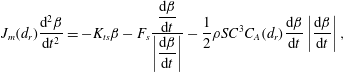 $$\begin{eqnarray}J_{m}(d_{r})\frac{\text{d}^{2}\unicode[STIX]{x1D6FD}}{\text{d}t^{2}}=-K_{ts}\unicode[STIX]{x1D6FD}-F_{s}\frac{\displaystyle \frac{\text{d}\unicode[STIX]{x1D6FD}}{\text{d}t}}{\displaystyle \left|\frac{\text{d}\unicode[STIX]{x1D6FD}}{\text{d}t}\right|}-\frac{1}{2}\unicode[STIX]{x1D70C}SC^{3}C_{A}(d_{r})\frac{\text{d}\unicode[STIX]{x1D6FD}}{\text{d}t}\left|\frac{\text{d}\unicode[STIX]{x1D6FD}}{\text{d}t}\right|,\end{eqnarray}$$
where
 $J_{m}(d_{r})$
is the moment of inertia of the projectile and is determined numerically,
$J_{m}(d_{r})$
is the moment of inertia of the projectile and is determined numerically,
 $K_{ts}$
is the torsional spring constant measured independently,
$K_{ts}$
is the torsional spring constant measured independently,
 $F_{s}$
is the solid friction torque determined by carrying out the experiment in air and
$F_{s}$
is the solid friction torque determined by carrying out the experiment in air and
 $C_{A}$
is the coefficient of angular dissipation and the fitting parameter. A typical fit is shown in figure 8(b), which nicely captures the data provided, and which yields an order of magnitude for
$C_{A}$
is the coefficient of angular dissipation and the fitting parameter. A typical fit is shown in figure 8(b), which nicely captures the data provided, and which yields an order of magnitude for
 $C_{A}\approx 10^{-2}$
.
$C_{A}\approx 10^{-2}$
.
By moving the position of the axis of rotation
 $d_{r}$
, the function
$d_{r}$
, the function
 $C_{A}(d_{r})$
is determined and plotted in figure 8(c).
$C_{A}(d_{r})$
is determined and plotted in figure 8(c).
 $C_{A}$
is maximum (
$C_{A}$
is maximum (
 $0.06$
) for extreme values of
$0.06$
) for extreme values of
 $d_{r}/C$
(5 % and
$d_{r}/C$
(5 % and
 $85\,\%$
) and it reaches its minimum for
$85\,\%$
) and it reaches its minimum for
 $d_{r}/C$
around
$d_{r}/C$
around
 $50\,\%$
.
$50\,\%$
.
In the impacting projectile experiment, the projectile rotates around its centre of gravity. Hence, for a projectile with a centre of gravity located at a distance
 $d_{g}$
from the leading edge
$d_{g}$
from the leading edge
 ${\mathcal{D}}_{t}$
is computed with a coefficient
${\mathcal{D}}_{t}$
is computed with a coefficient
 $C_{A}(d_{g})=C_{A}(d_{r}=d_{g})$
.
$C_{A}(d_{g})=C_{A}(d_{r}=d_{g})$
.

Figure 8. (a) Chronophotograph and sketch of the experiment used to determine the dissipative torque. The time delay between two frames is 0.24 s.
 $d_{r}$
defines the position of the axis of rotation, aligned with the
$d_{r}$
defines the position of the axis of rotation, aligned with the
 $z^{\prime }$
-axis. A torsional spring of constant
$z^{\prime }$
-axis. A torsional spring of constant
 $K_{ts}$
sets an equilibrium position. The angle
$K_{ts}$
sets an equilibrium position. The angle
 $\unicode[STIX]{x1D6FD}$
is the angle between the projectile at equilibrium and its current position. (b) Time evolution of the angle
$\unicode[STIX]{x1D6FD}$
is the angle between the projectile at equilibrium and its current position. (b) Time evolution of the angle
 $\unicode[STIX]{x1D6FD}$
fitted with a solution of the equation of motion (4.4) to determine the coefficient
$\unicode[STIX]{x1D6FD}$
fitted with a solution of the equation of motion (4.4) to determine the coefficient
 $C_{A}$
such that
$C_{A}$
such that
 ${\mathcal{D}}_{t}=(1/2)\unicode[STIX]{x1D70C}SC^{3}C_{A}(d_{r})\,(\text{d}\unicode[STIX]{x1D6FD}/\text{d}t)|\text{d}\unicode[STIX]{x1D6FD}/\text{d}t|$
. (c) Dependence of
${\mathcal{D}}_{t}=(1/2)\unicode[STIX]{x1D70C}SC^{3}C_{A}(d_{r})\,(\text{d}\unicode[STIX]{x1D6FD}/\text{d}t)|\text{d}\unicode[STIX]{x1D6FD}/\text{d}t|$
. (c) Dependence of
 $C_{A}$
with the position
$C_{A}$
with the position
 $d_{r}/C$
of the axis of rotation of the projectile, where
$d_{r}/C$
of the axis of rotation of the projectile, where
 $C$
is the length of the chord of the projectile.
$C$
is the length of the chord of the projectile.
5 Results and discussion
5.1 Solution of the equation of motion

Figure 9. Trajectories of the centre of mass of the projectile calculated from the numerical solution of the equations of motion at different values of the impact velocity (
 $U_{0}$
), and for different positions of the centre of gravity of the projectile (
$U_{0}$
), and for different positions of the centre of gravity of the projectile (
 $d_{g}/C$
). A trajectory is considered unstable if we have
$d_{g}/C$
). A trajectory is considered unstable if we have
 $\text{d}\unicode[STIX]{x1D703}/\text{d}t(t=0^{+})>0$
. Stable trajectories are boxed in green (d,e), unstable ones in red (a,b,c,f).
$\text{d}\unicode[STIX]{x1D703}/\text{d}t(t=0^{+})>0$
. Stable trajectories are boxed in green (d,e), unstable ones in red (a,b,c,f).
The equations of motion (4.1) can be solved using the parameters determined in the previous section and the initial conditions. Figure 9 presents a set of trajectories obtained after integrating numerically the equations for different impact velocities
 $U_{0}$
and various relative positions
$U_{0}$
and various relative positions
 $d_{g}/C$
of the centre of mass. The overall shapes of the trajectories are similar to those observed experimentally and reported in figure 2. Indeed, for a centre of gravity located close to the leading edge (
$d_{g}/C$
of the centre of mass. The overall shapes of the trajectories are similar to those observed experimentally and reported in figure 2. Indeed, for a centre of gravity located close to the leading edge (
 $d_{g}/C=18\,\%$
), the trajectories at both low and high impact velocity are straight – left-hand side of figure 9 (panels a,d). When the centre of mass is further from the leading edge (
$d_{g}/C=18\,\%$
), the trajectories at both low and high impact velocity are straight – left-hand side of figure 9 (panels a,d). When the centre of mass is further from the leading edge (
 $d_{g}/C=27\,\%$
), the trajectory remains straight at low velocity (9
e) but it adopts a y-shape at high velocity (9
b). Finally, for a centre of gravity far from the leading edge (
$d_{g}/C=27\,\%$
), the trajectory remains straight at low velocity (9
e) but it adopts a y-shape at high velocity (9
b). Finally, for a centre of gravity far from the leading edge (
 $d_{g}/C=44\,\%$
), the trajectory is U-shaped at all impact velocities (9
c,f).
$d_{g}/C=44\,\%$
), the trajectory is U-shaped at all impact velocities (9
c,f).
However, two discrepancies can be noted when comparing the observations in figure 2 to the numerical solutions in figure 9. First, for
 $d_{g}/C=44\,\%$
, there is no reduction of the dive depth for
$d_{g}/C=44\,\%$
, there is no reduction of the dive depth for
 $U_{0}=1.8~\text{m}~\text{s}^{-1}$
, which is due to the fact that the equations of motion do not take into account the formation of air cavities. Second, in the numerical solution, the motion is considered unstable if
$U_{0}=1.8~\text{m}~\text{s}^{-1}$
, which is due to the fact that the equations of motion do not take into account the formation of air cavities. Second, in the numerical solution, the motion is considered unstable if
 $\text{d}\unicode[STIX]{x1D703}/\text{d}t(t=0^{+})>0$
, that is, if the projectile deviates from its initial position
$\text{d}\unicode[STIX]{x1D703}/\text{d}t(t=0^{+})>0$
, that is, if the projectile deviates from its initial position
 $\unicode[STIX]{x1D703}_{0}$
away from the vertical (
$\unicode[STIX]{x1D703}_{0}$
away from the vertical (
 $\unicode[STIX]{x1D703}=0$
) just after impacting water. Although the trajectory obtained for
$\unicode[STIX]{x1D703}=0$
) just after impacting water. Although the trajectory obtained for
 $U_{0}=1.8~\text{m}~\text{s}^{-1}$
and
$U_{0}=1.8~\text{m}~\text{s}^{-1}$
and
 $d_{g}/C=18\,\%$
appears straight, it is found to be numerically unstable. This can be explained by taking into account the growth rate of the instability, which is addressed in the next subsection.
$d_{g}/C=18\,\%$
appears straight, it is found to be numerically unstable. This can be explained by taking into account the growth rate of the instability, which is addressed in the next subsection.
5.2 Critical velocity and growth time
As observed in figure 5(b), if the centre of mass of the projectile is located closer to the leading edge than the point of application of Archimedes’ force (
 $d_{p}>d_{g}$
), Archimedes’ torque is stabilizing (it tends to align the projectile with the vertical) whereas the lift and drag torques are destabilizing. Hence, we can define a critical velocity
$d_{p}>d_{g}$
), Archimedes’ torque is stabilizing (it tends to align the projectile with the vertical) whereas the lift and drag torques are destabilizing. Hence, we can define a critical velocity
 $U^{\ast }$
at which the destabilizing and the stabilizing torques balance. Since the drag and lift forces apply at the leading edge for small
$U^{\ast }$
at which the destabilizing and the stabilizing torques balance. Since the drag and lift forces apply at the leading edge for small
 $\unicode[STIX]{x1D6FC}$
(figure 7
c), the angular momentum equation (4.1) can be rewritten and solved for
$\unicode[STIX]{x1D6FC}$
(figure 7
c), the angular momentum equation (4.1) can be rewritten and solved for
 $U^{\ast }$
. This yields:
$U^{\ast }$
. This yields:
 $$\begin{eqnarray}U^{\ast }=\sqrt{\frac{2gV(d_{p}-d_{g})\sin \unicode[STIX]{x1D703}_{0}}{d_{g}S(C_{L}\cos \unicode[STIX]{x1D703}_{0}+C_{D}\sin \unicode[STIX]{x1D703}_{0})}},\end{eqnarray}$$
where
 $V$
is the volume of the projectile.
$V$
is the volume of the projectile.
For
 $U_{0}<U^{\ast }$
, the drag and lift torques are smaller than the stabilizing Archimedes torque so that the initial small angle between the vertical and the projectile chord decreases: projectiles align with the vertical and we have quasi-straight trajectories. For
$U_{0}<U^{\ast }$
, the drag and lift torques are smaller than the stabilizing Archimedes torque so that the initial small angle between the vertical and the projectile chord decreases: projectiles align with the vertical and we have quasi-straight trajectories. For
 $U_{0}>U^{\ast }$
, conversely, they deviate from the vertical (its initial angle
$U_{0}>U^{\ast }$
, conversely, they deviate from the vertical (its initial angle
 $\unicode[STIX]{x1D703}_{0}$
increases). As the motion proceeds, the velocity of the projectile decreases and Archimedes’ torque eventually takes over: the projectile aligns back with the vertical at the maximum depth of the dive and the motion is y-shaped.
$\unicode[STIX]{x1D703}_{0}$
increases). As the motion proceeds, the velocity of the projectile decreases and Archimedes’ torque eventually takes over: the projectile aligns back with the vertical at the maximum depth of the dive and the motion is y-shaped.
If the centre of mass of the projectile is located further from the leading edge than the point of application of Archimedes’ force (
 $d_{g}>d_{p}$
), all torques are destabilizing. The projectile keeps deviating from the vertical: the trajectory is U-shaped.
$d_{g}>d_{p}$
), all torques are destabilizing. The projectile keeps deviating from the vertical: the trajectory is U-shaped.
Overall, as
 $d_{g}$
is moved away from the leading edge, the critical velocity
$d_{g}$
is moved away from the leading edge, the critical velocity
 $U^{\ast }$
decreases until it vanishes for
$U^{\ast }$
decreases until it vanishes for
 $d_{g}=d_{p}$
. Additionally, when the impact angle
$d_{g}=d_{p}$
. Additionally, when the impact angle
 $\unicode[STIX]{x1D703}_{0}$
is small, as
$\unicode[STIX]{x1D703}_{0}$
is small, as
 $C_{L}\propto \unicode[STIX]{x1D6FC}^{1.507}$
(figure 6
b), it is interesting to note that the critical velocity diverges.
$C_{L}\propto \unicode[STIX]{x1D6FC}^{1.507}$
(figure 6
b), it is interesting to note that the critical velocity diverges.
Equation (5.1) is plotted in blue for two different initial angles
 $\unicode[STIX]{x1D703}_{0}$
(
$\unicode[STIX]{x1D703}_{0}$
(
 $0.3^{\circ }$
and
$0.3^{\circ }$
and
 $6^{\circ }$
) in figure 10: as one can expect, increasing the initial angle
$6^{\circ }$
) in figure 10: as one can expect, increasing the initial angle
 $\unicode[STIX]{x1D703}_{0}$
decreases the velocity necessary to deviate the trajectory (
$\unicode[STIX]{x1D703}_{0}$
decreases the velocity necessary to deviate the trajectory (
 $U^{\ast }$
decreased). When compared with data, one can note that although all the experimental points lying below the theoretical prediction for
$U^{\ast }$
decreased). When compared with data, one can note that although all the experimental points lying below the theoretical prediction for
 $U^{\ast }$
are observed to be stable (green points), motions can be observed to be stable even for
$U^{\ast }$
are observed to be stable (green points), motions can be observed to be stable even for
 $U_{0}>U^{\ast }$
(orange points).
$U_{0}>U^{\ast }$
(orange points).
For a fixed centre of mass located close to the leading edge (
 $d_{g}<d_{p}$
), an increase of impact velocity
$d_{g}<d_{p}$
), an increase of impact velocity
 $U_{0}$
leads to a transition from straight to y-shaped trajectories (path (1) in figure 10), as observed in figure 4(a). Similarly, when the centre of mass of the projectile is further from the leading edge (increasing (
$U_{0}$
leads to a transition from straight to y-shaped trajectories (path (1) in figure 10), as observed in figure 4(a). Similarly, when the centre of mass of the projectile is further from the leading edge (increasing (
 $d_{g}/C$
) at fixed impact velocity, we observe a first transition from straight to y-shaped trajectories and a second transition to U-shapes (path (2) on figure 10), as also reported in figure 4(b).
$d_{g}/C$
) at fixed impact velocity, we observe a first transition from straight to y-shaped trajectories and a second transition to U-shapes (path (2) on figure 10), as also reported in figure 4(b).

Figure 10. Stability diagram of a projectile impacting water at a velocity
 $U_{0}$
with its centre of mass located at a distance
$U_{0}$
with its centre of mass located at a distance
 $d_{g}$
from the leading edge. The critical velocity
$d_{g}$
from the leading edge. The critical velocity
 $U^{\ast }$
theoretically predicted is plotted in blue for impact angles
$U^{\ast }$
theoretically predicted is plotted in blue for impact angles
 $\unicode[STIX]{x1D703}_{0}$
between
$\unicode[STIX]{x1D703}_{0}$
between
 $0.3^{\circ }$
and
$0.3^{\circ }$
and
 $6^{\circ }$
. The area delimited by the curves for which the characteristic growth time of the instability
$6^{\circ }$
. The area delimited by the curves for which the characteristic growth time of the instability
 $\unicode[STIX]{x1D70F}_{i}$
equates to the characteristic time of the fall
$\unicode[STIX]{x1D70F}_{i}$
equates to the characteristic time of the fall
 $\unicode[STIX]{x1D70F}_{f}$
(i.e.
$\unicode[STIX]{x1D70F}_{f}$
(i.e.
 $\unicode[STIX]{x1D70F}_{i}/\unicode[STIX]{x1D70F}_{f}=1$
with
$\unicode[STIX]{x1D70F}_{i}/\unicode[STIX]{x1D70F}_{f}=1$
with
 $\unicode[STIX]{x0394}\unicode[STIX]{x1D703}=\unicode[STIX]{x03C0}/2$
) for
$\unicode[STIX]{x0394}\unicode[STIX]{x1D703}=\unicode[STIX]{x03C0}/2$
) for
 $\unicode[STIX]{x1D703}_{0}=0.3^{\circ }$
and
$\unicode[STIX]{x1D703}_{0}=0.3^{\circ }$
and
 $6^{\circ }$
, is shaded in yellow. Experimental points are the green dots (stable), orange triangles (transition) and red squares (unstable).
$6^{\circ }$
, is shaded in yellow. Experimental points are the green dots (stable), orange triangles (transition) and red squares (unstable).
In order to evaluate if the instability can develop, its characteristic growth time
 $\unicode[STIX]{x1D70F}_{i}$
(time necessary for a deviation of
$\unicode[STIX]{x1D70F}_{i}$
(time necessary for a deviation of
 $\unicode[STIX]{x0394}\unicode[STIX]{x1D703}$
from the vertical of the projectile) can be derived from a scaling analysis of the angular momentum conservation equation (4.1). Assuming
$\unicode[STIX]{x0394}\unicode[STIX]{x1D703}$
from the vertical of the projectile) can be derived from a scaling analysis of the angular momentum conservation equation (4.1). Assuming
 $\text{d}\unicode[STIX]{x1D703}^{2}/\text{d}t^{2}\approx \unicode[STIX]{x0394}\unicode[STIX]{x1D703}/\unicode[STIX]{x1D70F}_{i}^{2}$
, we find:
$\text{d}\unicode[STIX]{x1D703}^{2}/\text{d}t^{2}\approx \unicode[STIX]{x0394}\unicode[STIX]{x1D703}/\unicode[STIX]{x1D70F}_{i}^{2}$
, we find:
 $$\begin{eqnarray}\unicode[STIX]{x1D70F}_{i}=\sqrt{\frac{J\unicode[STIX]{x0394}\unicode[STIX]{x1D703}}{\frac{1}{2}d_{g}\unicode[STIX]{x1D70C}S{U_{0}}^{2}(\cos \unicode[STIX]{x1D703}_{0}C_{L}+\sin \unicode[STIX]{x1D703}_{0}C_{D})-\unicode[STIX]{x1D70C}gV\sin \unicode[STIX]{x1D703}_{0}(d_{p}-d_{g})}}.\end{eqnarray}$$
To evaluate the characteristic time of the fall
 $\unicode[STIX]{x1D70F}_{f}$
, we suppose that the motion is straight and that the projectile is only subjected to drag (Cohen et al.
Reference Cohen, Darbois-Texier, Dupeux, Brunel, Quéré and Clanet2014). Integrating the force balance, we get:
$\unicode[STIX]{x1D70F}_{f}$
, we suppose that the motion is straight and that the projectile is only subjected to drag (Cohen et al.
Reference Cohen, Darbois-Texier, Dupeux, Brunel, Quéré and Clanet2014). Integrating the force balance, we get:
 $$\begin{eqnarray}U(t)=\widetilde{U}\sqrt{\frac{1-\bar{\unicode[STIX]{x1D70C}}}{\bar{\unicode[STIX]{x1D70C}}}}\tan \left(\arctan \left(\frac{U_{0}}{\widetilde{U}}\sqrt{\frac{\bar{\unicode[STIX]{x1D70C}}}{1-\bar{\unicode[STIX]{x1D70C}}}}\right)-\frac{1-\bar{\unicode[STIX]{x1D70C}}}{\bar{\unicode[STIX]{x1D70C}}}\frac{g}{\widetilde{U}}t\right),\end{eqnarray}$$
where
 $\widetilde{U}=\sqrt{2gm/\unicode[STIX]{x1D70C}SC_{D}}$
is the characteristic velocity of the fall and
$\widetilde{U}=\sqrt{2gm/\unicode[STIX]{x1D70C}SC_{D}}$
is the characteristic velocity of the fall and
 $\bar{\unicode[STIX]{x1D70C}}$
the relative density of the projectile. As
$\bar{\unicode[STIX]{x1D70C}}$
the relative density of the projectile. As
 $U(\unicode[STIX]{x1D70F}_{f})=0$
, using (5.3), we find
$U(\unicode[STIX]{x1D70F}_{f})=0$
, using (5.3), we find
 $\unicode[STIX]{x1D70F}_{f}$
to be:
$\unicode[STIX]{x1D70F}_{f}$
to be:
 $$\begin{eqnarray}\unicode[STIX]{x1D70F}_{f}=\frac{\widetilde{U}}{g}\frac{\bar{\unicode[STIX]{x1D70C}}}{1-\bar{\unicode[STIX]{x1D70C}}}\arctan \left(\frac{U_{0}}{\widetilde{U}}\sqrt{\frac{\bar{\unicode[STIX]{x1D70C}}}{1-\bar{\unicode[STIX]{x1D70C}}}}\right).\end{eqnarray}$$
Using equations (5.2) and (5.4), the ratio
 $\unicode[STIX]{x1D70F}_{i}/\unicode[STIX]{x1D70F}_{f}$
is computed and plotted when equal to 1 for
$\unicode[STIX]{x1D70F}_{i}/\unicode[STIX]{x1D70F}_{f}$
is computed and plotted when equal to 1 for
 $\unicode[STIX]{x0394}\unicode[STIX]{x1D703}=\unicode[STIX]{x03C0}/2$
in figure 10 for different values of the impact angle
$\unicode[STIX]{x0394}\unicode[STIX]{x1D703}=\unicode[STIX]{x03C0}/2$
in figure 10 for different values of the impact angle
 $\unicode[STIX]{x1D703}_{0}$
. Below this curve, we have
$\unicode[STIX]{x1D703}_{0}$
. Below this curve, we have
 $\unicode[STIX]{x1D70F}_{f}<\unicode[STIX]{x1D70F}_{i}$
and the instability has no time to develop: the motion, when unstable, can however follow a straight trajectory – a regime that corresponds well with the orange data. This is the case for
$\unicode[STIX]{x1D70F}_{f}<\unicode[STIX]{x1D70F}_{i}$
and the instability has no time to develop: the motion, when unstable, can however follow a straight trajectory – a regime that corresponds well with the orange data. This is the case for
 $d_{g}/C=18\,\%$
and
$d_{g}/C=18\,\%$
and
 $U_{0}=1.8~\text{m}~\text{s}^{-1}$
, where the trajectory is experimentally found to be stable (figure 2
a) but numerically unstable (figure 9
a).
$U_{0}=1.8~\text{m}~\text{s}^{-1}$
, where the trajectory is experimentally found to be stable (figure 2
a) but numerically unstable (figure 9
a).
5.3 Quantitative comparison and dive depth
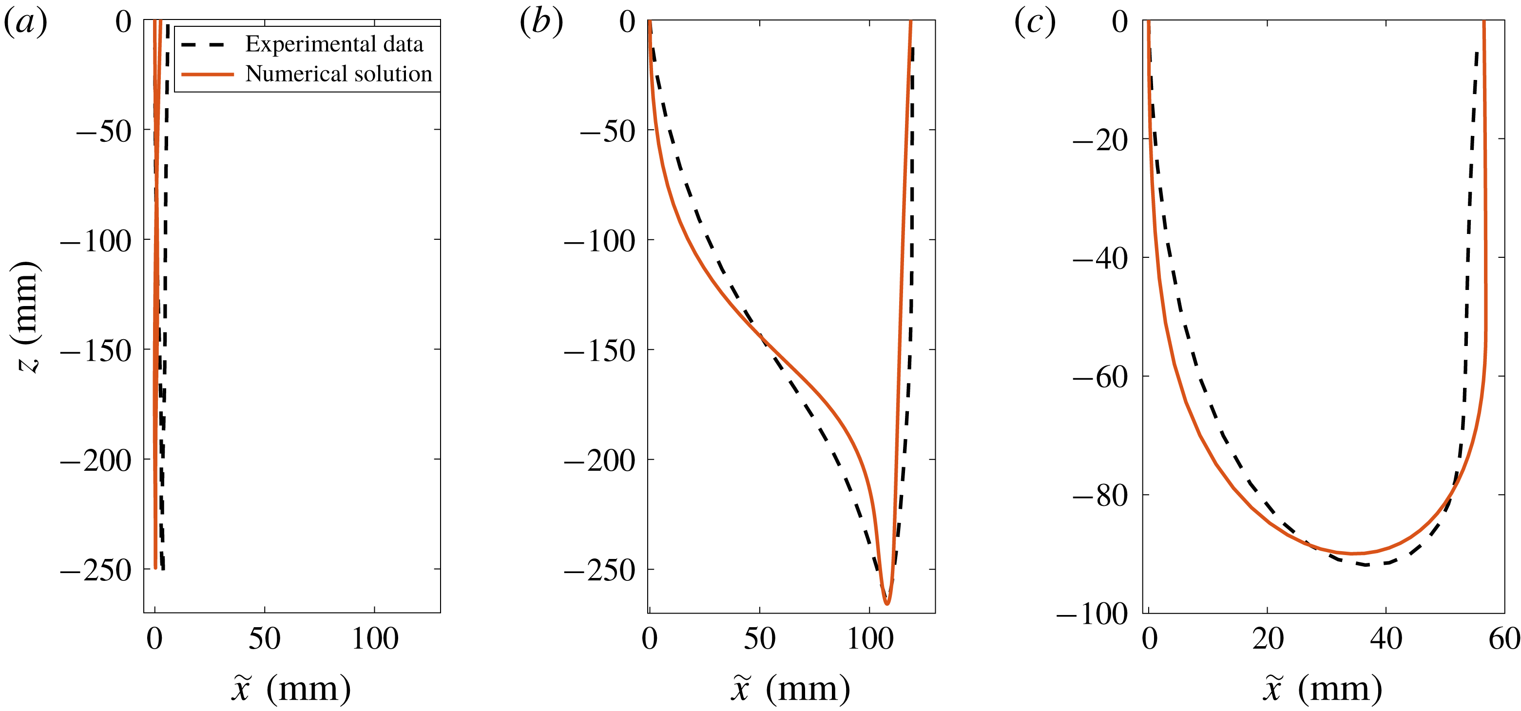
Figure 11. Trajectories of the centre of mass of different projectiles. Solid line is the numerical solution of the equation of motion and the dashed line is the experimental trajectory. The fitting parameter for the numerical solution is the angle
 $\unicode[STIX]{x1D703}_{0}$
between the vertical and the chord of the projectile at impact. (a) Straight trajectory for
$\unicode[STIX]{x1D703}_{0}$
between the vertical and the chord of the projectile at impact. (a) Straight trajectory for
 $d_{g}/C=18\,\%$
and
$d_{g}/C=18\,\%$
and
 $U_{0}=0.94~\text{m}~\text{s}^{-1}$
.
$U_{0}=0.94~\text{m}~\text{s}^{-1}$
.
 $\unicode[STIX]{x1D703}_{0}=2^{\circ }$
. (b) The y-shaped trajectory for
$\unicode[STIX]{x1D703}_{0}=2^{\circ }$
. (b) The y-shaped trajectory for
 $d_{g}/C=27\,\%$
and
$d_{g}/C=27\,\%$
and
 $U_{0}=1.25~\text{m}~\text{s}^{-1}$
.
$U_{0}=1.25~\text{m}~\text{s}^{-1}$
.
 $\unicode[STIX]{x1D703}_{0}=9^{\circ }$
. (c) U-shaped trajectory for
$\unicode[STIX]{x1D703}_{0}=9^{\circ }$
. (c) U-shaped trajectory for
 $d_{g}/C=44\,\%$
and
$d_{g}/C=44\,\%$
and
 $U_{0}=0.95~\text{m}~\text{s}^{-1}$
.
$U_{0}=0.95~\text{m}~\text{s}^{-1}$
.
 $\unicode[STIX]{x1D703}_{0}=5.5^{\circ }$
.
$\unicode[STIX]{x1D703}_{0}=5.5^{\circ }$
.
Quantitatively, one experimental trajectory of each type is fitted with the corresponding numerical solution of the equations of motion in figure 11. For straight (figure 11
a), y-shaped (figure 11
b) and U-shaped (figure 11
c) trajectories, the overall shape of the numerical solution, as well as the maximum depth and the maximum horizontal distance travelled, are in good agreement with the observed trajectories. The small discrepancies observed for the y-shape and the U-shape can be attributed to the fact that the only fitting parameter is the initial angle
 $\unicode[STIX]{x1D703}_{0}$
.
$\unicode[STIX]{x1D703}_{0}$
.

Figure 12. Comparison between the numerically predicted depth
 $h$
of the dive and experimental data. Shaded areas are the numerically determined depths for impact angle
$h$
of the dive and experimental data. Shaded areas are the numerically determined depths for impact angle
 $\unicode[STIX]{x1D703}_{0}$
ranging from
$\unicode[STIX]{x1D703}_{0}$
ranging from
 $0.3^{\circ }$
and
$0.3^{\circ }$
and
 $6^{\circ }$
. Filled dots are experimental data for different positions of the centre of gravity and mass of the projectile when no cavity is formed at the water entry:
$6^{\circ }$
. Filled dots are experimental data for different positions of the centre of gravity and mass of the projectile when no cavity is formed at the water entry:
 $d_{g}/C=24\,\%$
,
$d_{g}/C=24\,\%$
,
 $m=6.7~\text{g}$
,
$m=6.7~\text{g}$
,
 $d_{g}/C=27\,\%$
,
$d_{g}/C=27\,\%$
,
 $m=6.85~\text{g}$
,
$m=6.85~\text{g}$
,
 $d_{g}/C=37\,\%$
,
$d_{g}/C=37\,\%$
,
 $m=6.32~\text{g}$
,
$m=6.32~\text{g}$
,
 $d_{g}/C=44\,\%$
,
$d_{g}/C=44\,\%$
,
 $m=6.4~\text{g}$
. Empty dots are experimental data for projectile entraining an air cavity at water entry.
$m=6.4~\text{g}$
. Empty dots are experimental data for projectile entraining an air cavity at water entry.
The depth
 $h$
of the dive, can be determined numerically when the impact velocity
$h$
of the dive, can be determined numerically when the impact velocity
 $U_{0}$
is varied for a range of impact angles
$U_{0}$
is varied for a range of impact angles
 $\unicode[STIX]{x1D703}_{0}$
and it is plotted in coloured area in figure 12. The predicted depth is compared with data for different positions of the centre of mass
$\unicode[STIX]{x1D703}_{0}$
and it is plotted in coloured area in figure 12. The predicted depth is compared with data for different positions of the centre of mass
 $d_{g}$
. The agreement is good, except when an air cavity is entrained, an ingredient not present in the model – the dive depth in this case being naturally found to be significantly smaller than predicted.
$d_{g}$
. The agreement is good, except when an air cavity is entrained, an ingredient not present in the model – the dive depth in this case being naturally found to be significantly smaller than predicted.
To further understand the saturation in depth reached by the streamlined projectile, we can obtain the theoretical variation of depth of a projectile
 $z_{g}$
with time
$z_{g}$
with time
 $t$
by integrating equation (5.3):
$t$
by integrating equation (5.3):
 $$\begin{eqnarray}\frac{z_{g}(t)}{{\mathcal{L}}}=\log \left\{\cos \left[\arctan \left(\frac{U_{0}}{\widetilde{U}}\right)-\frac{1-\bar{\unicode[STIX]{x1D70C}}}{\bar{\unicode[STIX]{x1D70C}}}\frac{gt}{\widetilde{U}}\right]\right\},\end{eqnarray}$$
where
 ${\mathcal{L}}=2m/\unicode[STIX]{x1D70C}SC_{D}$
is the characteristic length of the dive. This relation can be evaluated at
${\mathcal{L}}=2m/\unicode[STIX]{x1D70C}SC_{D}$
is the characteristic length of the dive. This relation can be evaluated at
 $t=\unicode[STIX]{x1D70F}_{f}$
to get the maximal depth of a straight dive, which is plotted by the dotted line in figure 13. Furthermore, once the instability is established, the maximum depth of the dive will rather be set by
$t=\unicode[STIX]{x1D70F}_{f}$
to get the maximal depth of a straight dive, which is plotted by the dotted line in figure 13. Furthermore, once the instability is established, the maximum depth of the dive will rather be set by
 $\unicode[STIX]{x1D70F}_{i}$
, so that we expect
$\unicode[STIX]{x1D70F}_{i}$
, so that we expect
 $h\sim z_{g}(\unicode[STIX]{x1D70F}_{i})$
. This distance is plotted by the dashed line in figure 13. Finally, we can notice that the curve
$h\sim z_{g}(\unicode[STIX]{x1D70F}_{i})$
. This distance is plotted by the dashed line in figure 13. Finally, we can notice that the curve
 $z_{g}(\min (\unicode[STIX]{x1D70F}_{i},\unicode[STIX]{x1D70F}_{f}))$
matches both the numerical and experimental data well.
$z_{g}(\min (\unicode[STIX]{x1D70F}_{i},\unicode[STIX]{x1D70F}_{f}))$
matches both the numerical and experimental data well.

Figure 13. Comparison between the theoretical prediction for the dive depth and both numerical and experimental data. Shaded areas are the numerically determined depths for impact angles
 $\unicode[STIX]{x1D703}_{0}$
ranging from
$\unicode[STIX]{x1D703}_{0}$
ranging from
 $0.3^{\circ }$
and
$0.3^{\circ }$
and
 $6^{\circ }$
. Filled dots are data for a centre of mass located at
$6^{\circ }$
. Filled dots are data for a centre of mass located at
 $d_{g}/C=24\,\%$
and a mass
$d_{g}/C=24\,\%$
and a mass
 $m=6.7~\text{g}$
. Dotted line is the theoretical maximum depth of the dive for a straight trajectory, i.e.
$m=6.7~\text{g}$
. Dotted line is the theoretical maximum depth of the dive for a straight trajectory, i.e.
 $z_{g}(\unicode[STIX]{x1D70F}_{f})$
using equation (5.5). Dashed line is the theoretical depth
$z_{g}(\unicode[STIX]{x1D70F}_{f})$
using equation (5.5). Dashed line is the theoretical depth
 $z_{g}(\unicode[STIX]{x1D70F}_{i})$
of a straight dive reached at the time
$z_{g}(\unicode[STIX]{x1D70F}_{i})$
of a straight dive reached at the time
 $\unicode[STIX]{x1D70F}_{i}$
at which the instability has developed. Solid line is
$\unicode[STIX]{x1D70F}_{i}$
at which the instability has developed. Solid line is
 $z_{g}(\min (\unicode[STIX]{x1D70F}_{i},\unicode[STIX]{x1D70F}_{f}))$
.
$z_{g}(\min (\unicode[STIX]{x1D70F}_{i},\unicode[STIX]{x1D70F}_{f}))$
.
Therefore, we can conclude that: First, when
 $\unicode[STIX]{x1D70F}_{f}<\unicode[STIX]{x1D70F}_{i}$
, the motion is stable, the trajectory is quasi-straight and the maximum depth is
$\unicode[STIX]{x1D70F}_{f}<\unicode[STIX]{x1D70F}_{i}$
, the motion is stable, the trajectory is quasi-straight and the maximum depth is
 $z_{g}(\unicode[STIX]{x1D70F}_{f})$
. Second, when
$z_{g}(\unicode[STIX]{x1D70F}_{f})$
. Second, when
 $\unicode[STIX]{x1D70F}_{f}>\unicode[STIX]{x1D70F}_{i}$
, the instability has time to grow, the projectile has a y-shaped or U-shaped trajectory and the maximum depth of the dive is
$\unicode[STIX]{x1D70F}_{f}>\unicode[STIX]{x1D70F}_{i}$
, the instability has time to grow, the projectile has a y-shaped or U-shaped trajectory and the maximum depth of the dive is
 $z_{g}(\unicode[STIX]{x1D70F}_{i})$
.
$z_{g}(\unicode[STIX]{x1D70F}_{i})$
.
6 Conclusion
We studied the trajectories of floating axisymmetric streamlined bodies impacting water with an initial vertical velocity. Both the depth of the dive and the morphology of the trajectory are found to be highly dependent on the position of the centre of gravity of the projectile. When the centre of mass is located closer to the leading edge than the point of application of Archimedes’ force (
 $d_{g}<d_{p}$
), the trajectory is straight at low impact velocity. For higher velocities, the trajectories become y-shaped. For
$d_{g}<d_{p}$
), the trajectory is straight at low impact velocity. For higher velocities, the trajectories become y-shaped. For
 $d_{g}>d_{p}$
, the motion is always unstable and the trajectory has a U-shape.
$d_{g}>d_{p}$
, the motion is always unstable and the trajectory has a U-shape.
For both the y-path and U-path, the instability saturates the depth of the dive before the appearance of an air cavity at the water entry and reduces the depth of the dive.
For
 $d_{g}<d_{p}$
, the critical velocity
$d_{g}<d_{p}$
, the critical velocity
 $U^{\ast }$
is defined no matter what the position of the centre of gravity
$U^{\ast }$
is defined no matter what the position of the centre of gravity
 $d_{g}$
. Hence, the stability of the trajectory cannot be ensured for all impact velocities simply by moving the position of the centre of gravity. The motion has to be stabilized by the addition of fins on the projectile.
$d_{g}$
. Hence, the stability of the trajectory cannot be ensured for all impact velocities simply by moving the position of the centre of gravity. The motion has to be stabilized by the addition of fins on the projectile.
Acknowledgements
We thank the Direction Générale de l’Armement (DGA) for their financial support to the project. We are grateful to R. E. Cohen and G. McKinley for their involvement in the early stages of the project. We thank R. Labbé and C. Frot for their help in the design of the experimental set-up. We also thank Z. Pan and L. Masson for the first observations of the y-shape trajectories.


