3.1. Fluid and particle velocity

Here and in the following, the streamwise and wall-normal coordinates are indicated by $x$ and $y$, respectively, and $u$ and $v$ indicate the respective velocity components. These are Reynolds decomposed as $u = \langle u\rangle + u'$ and $v = \langle v\rangle + v'$, where angle brackets denote the time average and the prime denotes the fluctuating part. Subscripts f and p denote quantities referring to fluid and particles, respectively, and the subscript $f|p$ denotes fluid quantities interpolated at the particle location. In figures 7 and 8, the particle-laden and unladen fluid velocity statistics are compared to turbulent boundary-layer measurements by De Graaff & Eaton (Reference De Graaff and Eaton2000) at a similar Reynolds number ($Re_\theta = 1430$). The particle-laden and unladen fluid velocity profiles overlap within experimental uncertainty, indicating that significant two-way momentum coupling between the particles and fluid is not present. From the mean velocity profile, the friction velocity is determined by iterative fitting, with the von Kármán constant $\kappa = 0.41$ and the additive constant $B = 5.5$. The Reynolds stress profiles show some discrepancies in the magnitudes of the peak stresses due to the non-canonical features of the channel design (unconventional forcing, limited channel width) and limited spatial resolution. Physical parameters of the water channel and the boundary-layer properties are reported in table 3.

Figure 7. Mean streamwise velocity profile of the particle-laden (black dots) and unladen (red dots) fluid, in (a) outer units and (b) wall units. The dashed line in (b) indicates the logarithmic-law fit. The profile is compared with De Graaff & Eaton (Reference De Graaff and Eaton2000) in (b), shown in blue open circles.

Figure 8. Profiles of particle-laden (black dots) and unladen (red dots) streamwise turbulent normal stress (a), wall-normal normal stress (b) and shear stress (c) of the fluid in wall units. The profiles are compared with De Graaff & Eaton (Reference De Graaff and Eaton2000) shown in blue open circles.

Table 3. Physical parameters of the water channel and boundary-layer properties. $U_\infty$ is the free-stream velocity, H is the water depth, W is the channel width, $\delta _{99}$ is the boundary-layer thickness and $u_\tau$ is the shear velocity. The boundary thickness is defined such that $u(\delta _{99}) = 0.99U_\infty$; $Re = U_\infty H/\nu$, $Re_\tau = u_\tau \delta _{99}/\nu$ and $Re_\theta = U_\infty \theta /\nu$ are the free-stream, friction and momentum thickness Reynolds numbers, respectively. Standard water properties at $22\,^{\circ }\textrm {C}$ are used in the calculations.

Profiles of particle velocity are obtained by defining wall-normal layers (bins) and taking the mean of particle velocities within each. Particles are more numerous near the wall and sparser in the outer region (approximately following a power law, see § 3.6), thus the bins are logarithmically spaced to equalize the numbers of particles in each, as well as to capture the high shear in the near-wall region. The mean streamwise and wall-normal particle velocity profiles are shown in figure 9. In the free stream, the particle streamwise velocity is very similar to the fluid's (figure 9a), as expected since there the particles are in equilibrium with a steady flow having negligible fluctuations. Closer to the wall ($y^{+} \lesssim 200$) the particles generally lag the fluid, due to their inertia in responding to turbulence. Past experiments found that mean velocity of inertial particles exceeded that of the fluid in the viscous sublayer; see Kaftori et al. (Reference Kaftori, Hetsroni and Banerjee1995a), Righetti & Romano (Reference Righetti and Romano2004) and Ebrahimian et al. (Reference Ebrahimian, Sanders and Ghaemi2019). The present PIV resolution does not allow reliable measurements at such small heights, but the canonical shape of the boundary-layer profile suggests that the lag is vanishing approaching the wall. We remark that those previous studies considered smaller particles (in wall units) whose centroid could reach closer to the wall.

Figure 9. Wall-normal profiles of streamwise (a) and wall-normal (b) mean particle velocity (red crosses) compared with the mean fluid velocity (black dots).

The vertical velocity profile (figure 9b) shows that in the free stream the particles settle through the fluid at a speed close to the still-fluid terminal velocity. This is again consistent with the fact that particles at those heights fall through a quasi-laminar flow. For $y^{+} \lesssim 200$ (the same range for which particles lag the fluid streamwise velocity), the vertical velocity decays in magnitude, but remains negative. We note that a downward mean particle velocity is expected under equilibrium conditions, i.e. when the wall-normal turbulent flux balances the gravitational settling (Rouse Reference Rouse1937; Prandtl Reference Prandtl1952). Using the concentration measurements (see § 3.6), we estimate the total vertical flux to be several orders of magnitude smaller than the streamwise flux, confirming approximate equilibrium conditions. The Rouse–Prandtl theory, however, assumes a constant settling velocity (generally taken to be equal to the still-fluid terminal velocity) throughout the boundary layer, while here it shrinks to vanishingly small values approaching the wall. We investigate the roots of this effect, as well as the streamwise velocity lag, in the following.

3.2. Slip velocity

The reduced streamwise velocity of the particles has been often attributed to the preferential sampling of slow fluid regions (Kaftori et al. Reference Kaftori, Hetsroni and Banerjee1995a; Kiger & Pan Reference Kiger and Pan2002). We investigate this issue first by separating the mean slip velocity ($\langle u_p\rangle - \langle u_f\rangle$) in two separate contributions: the ‘particle-conditioned’ slip velocity, i.e. the mean slip velocity at the particle location, $\langle u_p - u_{f|p}\rangle$, and the ‘apparent’ slip velocity due to the oversampling of fluid regions faster or slower than the average, $\langle u_{f|p}\rangle - \langle u_f\rangle$ (Kiger & Pan Reference Kiger and Pan2002)

(3.1)\begin{equation} \langle u_p\rangle - \langle u_f\rangle = \langle u_p - u_{f|p}\rangle + \langle u_{f|p}\rangle - \langle u_f\rangle . \end{equation}

Figure 10(a) displays both contributions. (We only report the slip velocity down to the location of the PIV vector closest to the wall, to avoid extrapolation.) It indicates that, for $y^{+} > 20$, the particles do oversample fluid regions with negative streamwise fluctuations ($\langle u_{f|p}\rangle - \langle u_f\rangle < 0$). Closer to the wall, however, the particle-conditioned slip plays a dominant role in determining the particle lag from the fluid: the term $\langle u_p - u_{f|p}\rangle$ becomes larger in magnitude than $\langle u_{f|p}\rangle - \langle u_f\rangle$. This is consistent with the recent findings of Berk & Coletti (Reference Berk and Coletti2020) who considered solid particles in air at much larger $Re_\tau$ and a broad range of ${{\textit {St}}}^{+}$.

Figure 10. Wall-normal profiles of mean streamwise (a) and wall-normal (b) particle slip velocity, separated into the particle-conditioned mean slip (blue circles) and the apparent mean slip (red crosses).

A similar decomposition can be carried out for the vertical velocity component, noting that $\langle v_f\rangle = 0$:

(3.2)\begin{equation} \langle v_p\rangle = \langle v_p - v_{f|p}\rangle + \langle v_{f|p}\rangle, \end{equation}

which highlights the separate contributions of the particle-conditioned slip and the vertical fluid velocity at the particle location. Figure 10(b) shows that the first term on the right-hand side dominates in the free stream and decreases approaching the wall. The second term, representing the preferential sampling of upward/downward fluid fluctuations, is negligible in the free stream and it becomes comparable to the first term as the wall is approached. In particular, particles near the wall oversample upward fluid motions ($\langle v_{f|p}\rangle > 0$). This is consistent with their tendency of favouring negative streamwise fluctuations, which are correlated with upward fluctuations in a turbulent shear flow. This point will be further discussed in § 3.4. In general, throughout the boundary layer, the effect of the turbulence on the particle settling is opposite to what one would expect from homogeneous turbulence studies, where the predominant effect is the enhancement of settling speed by preferential sweeping (Wang & Maxey Reference Wang and Maxey1993; Petersen et al. Reference Petersen, Baker and Coletti2019).

The mean particle-conditioned slip velocity can be used to define profiles of particle Reynolds numbers, $Re_{p,u_{slip}}=\langle u_p-u_{f|p}\rangle D_p/\nu$ and $Re_{p,v_{slip}}=\langle v_p-v_{f|p}\rangle D_p/\nu$, shown in figure 11. Given the observed ranges, the particle wakes are likely to extend for less than one diameter (Rimon & Cheng Reference Rimon and Cheng1969). At the present volume fraction, particles are hardly ever found so close to each other, indicating that the momentum coupling between particles can be assumed to be negligible. However, the Reynolds numbers are well into the nonlinear drag regime, especially in the near-wall region. While drag corrections are available (Clift et al. Reference Clift, Grace and Weber2005), those are developed for steady/quiescent flows. In a turbulent flow laden with particles at finite $Re_p$, the nonlinearities undermine the use of superposition (assumed in the derivation of the particle equation of motion, Maxey & Riley Reference Maxey and Riley1983), making the particle–fluid dynamics challenging to capture with point-particle simulations (Wang et al. Reference Wang, Fong, Coletti, Capecelatro and Richter2019).

Figure 11. Profiles of mean instantaneous particle Reynolds number based on the particle-conditioned streamwise (blue circles) and wall-normal (red crosses) slip velocity.

The instantaneous slip experienced by the particles with respect to the surrounding fluid is related to their ability to retain memory of the flow events experienced at previous times. Thus, one might infer that the gravitational drift plays a major role in determining the streamwise slip velocity, as the settling particles cross flow trajectories and attain large relative velocities with respect to the fluid. This view is certainly valid in homogeneous turbulence (e.g. Csanady Reference Csanady1963; Elghobashi & Truesdell Reference Elghobashi and Truesdell1992). In a turbulent boundary layer, however, the tendency of the particles to sample slow flow regions, combined with the mean wall-normal velocity gradient, leads to a different outcome. Let us consider separately the mean streamwise velocity profile for ascending and descending particles; that is, particles with positive and negative instantaneous vertical velocity, respectively. Figure 12(a) shows that ascending particles, on average, move slower than the fluid and account for most of the mean slip velocity reported above; while descending particles roughly match the mean fluid velocity in the outer layer. This trend, in agreement with Kiger & Pan (Reference Kiger and Pan2002) and van Hout (Reference van Hout2011), is explained by the fact that ascending particles come from slower-moving regions of the flow nearer to the wall, and therefore have lower streamwise velocities. Therefore, unlike in homogeneous flows, it is the ascending particles suspended by the turbulence that determine the large slip velocity, rather than the descending ones that settle due to gravity. Remarkably, the vertical velocity of the ascending particles is comparable in magnitude to that of the descending ones, both being the order of the friction velocity. As the descending particles near the wall are more numerous, their contributions dominate the statistics and the mean vertical velocity of the dispersed phase is negative.

Figure 12. Profiles of mean streamwise (a) and wall-normal (b) particle velocity conditioned on ascending (red crosses) and descending (blue circles) particles compared to the fluid velocity (black dots).

3.3. Reynolds stresses

Profiles of particle and fluid Reynolds stresses are compared in figure 13. The streamwise normal stress of the particles are comparable to that of the fluid, while the particle wall-normal normal stress and shear stress exceed that of the fluid in the range $20 \lesssim y^{+} \lesssim 200$. Qualitatively similar results were reported for particles in water (Kaftori, Hetsroni & Banerjee Reference Kaftori, Hetsroni and Banerjee1995b; van Hout Reference van Hout2011) and in air (e.g. Tanière et al. Reference Tanière, Oesterlé and Monnier1997; Fong, Amili & Coletti Reference Fong, Amili and Coletti2019). The relatively large particle velocity fluctuations are interpreted as a consequence of the spread in momentum of particles with different pathways, retaining memory of their interactions with disparate flow structures. This in turn results in particles often being surrounded by fluid with velocity different from their own, contributing to the instantaneous slip reported above.

Figure 13. Wall-normal profiles of the Reynolds stresses of the particles (red crosses) and fluid (black dots) normalized by the squared shear velocity.

To explore the particle–turbulence interaction, we again condition the fluid statistics on the location of ascending and descending particles. The Reynolds shear stresses are of special interest: they feature in the turbulence production and represent the statistical signature of the instantaneous sweep and ejection events that are believed to play a crucial role in the particle transport (Marchioli & Soldati Reference Marchioli and Soldati2002). Figure 14(a) displays the fluid Reynolds shear stress evaluated at the locations of ascending and descending particles, while figure 14(b) shows the ‘particle Reynolds shear stress’ associated with ascending and descending particles. The ascending particles appear to sample regions with much larger fluid shear stress magnitudes compared to the descending particles, while the shear stress magnitudes of ascending and descending particles themselves are nearly the same. That suggests that the motion of the former is strongly driven by turbulent ejection events, while the latter have a weaker relation to sweep events.

Figure 14. Wall-normal profiles of the Reynolds shear stress of (a) the fluid velocity at particle locations and (b) the particle velocity, conditioned on ascending and descending particles (red crosses and blue circles, respectively). The profiles are compared to the overall fluid shear stress profile (black dots).

3.4. Quadrant analysis

Previous work (e.g. Niño & Garcia Reference Niño and Garcia1996; Kiger & Pan Reference Kiger and Pan2002; Marchioli & Soldati Reference Marchioli and Soldati2002; van Hout Reference van Hout2011) found evidence that inertial particles are strongly affected by sweep and ejection events in the turbulent boundary layer. Sweeps are identified as simultaneous $u_f' > 0$ and $v_f' < 0$ events (fourth quadrant of the $u_f'$–$v_f'$ plane, or Q4) and ejections as simultaneous $u_f' < 0$ and $v_f' > 0$ (second quadrant, or Q2). They are often associated with coherent structures in wall turbulence, such as streamwise rollers and hairpin vortices (Robinson Reference Robinson1991). We first plot in figure 15 the joint PDF of streamwise and wall-normal fluid velocity fluctuations: for the near-wall region ($y^{+} < 100$, figure 15a) and farther away from the wall ($y^{+} > 100$, figure 15b). As expected, sweeps and ejections are dominant near the wall, whereas away from the wall the fluctuations are weaker and there are no dominant quadrants. We then consider the quadrant events at the location of ascending and descending particles, in the near-wall and outer regions. Near the wall, ascending particles are found to strongly oversample ejection events (figure 15c), supporting the view that ejections are a major mechanism driving particle resuspension. Even in the outer region, although the ejections themselves are weaker, ascending particles still occupy the second quadrant almost exclusively (figure 15d). In contrast, descending particles are found to oversample sweep events near the wall, but the preference is weaker (figure 15e), and in the outer region, descending particles do not preferentially sample any quadrant (figure 15f). This indicates that sweeps weakly influence the descent of particles towards the wall, while ejections are a key factor in lifting the particles away from the wall.

Figure 15. Joint PDFs of streamwise and wall-normal fluctuating fluid velocities for $y^{+} < 100$ (a) and $y^{+} > 100$ (b). Joint PDFs of streamwise and wall-normal fluctuating fluid velocities at particle locations for $y^{+} < 100$ (c,e) and $y^{+} > 100$ (d,f) conditioned on whether the particle is ascending (c,d) or descending (e,f).

The prevalence of fluid ejection over sweeps in influencing particle transport was reported by previous studies focused on heavy particles suspended in horizontal wall-bounded flows over a wide range of physical parameters (Kiger & Pan Reference Kiger and Pan2002; van Hout Reference van Hout2011; Li et al. Reference Li, Wang, Liu, Chen and Zheng2012; Zhu et al. Reference Zhu, Pan, Wang, Liang and Ji2019; Berk & Coletti Reference Berk and Coletti2020). This is in contrast with configurations in which gravity does not participate to the wall-normal transport: in no-gravity simulations (e.g. Marchioli & Soldati Reference Marchioli and Soldati2002) and in vertical channel flow experiments (e.g. Fong et al. Reference Fong, Amili and Coletti2019) sweep events crucially contribute to the turbophoretic drift that produces a multi-fold increase in near-wall concentration. In horizontal particle-laden flows, by contrast, the near-wall concentration has been found to be smaller than what predicted by the Rouse–Prandtl equilibrium theory (Kiger & Pan Reference Kiger and Pan2002; Zhu et al. Reference Zhu, Pan, Wang, Liang and Ji2019; Berk & Coletti Reference Berk and Coletti2020). In § 3.6 we will show this to be the case also in the present configuration. Because the Rouse–Prandtl theory does not account for turbophoresis, we deduce the latter is not playing a significant role in the particle transport for the present conditions, despite ${{\textit {St}}}^{+}$ being in the turbophoretic regime according to point-particle simulations without gravity (see, e.g. Bernardini Reference Bernardini2014). This could be partly due to the relatively large size of our particles, which influences the ability of inner-layer streamwise vortices to accumulate them at the wall. However, considering the findings of previous studies with much smaller particles (e.g., Berk & Coletti Reference Berk and Coletti2020), the more likely reason is that gravitational drift disrupts the particle interaction with coherent turbulent motions.

3.5. Particle diffusion

The question of dispersion is central in particle-laden flows. A large body of experimental and numerical work in homogeneous turbulence has established that heavy particles disperse differently from tracers due to two distinct and competing effects. Particle inertia increases the integral time scale of their Lagrangian velocity autocorrelation, and hence their diffusivity, due to the finite response time (Squires & Eaton Reference Squires and Eaton1991; Wang & Stock Reference Wang and Stock1993; Jung, Yeo & Lee Reference Jung, Yeo and Lee2008). Meanwhile, particle drift due to gravity or other body forces causes them to cross fluid trajectories with consequent decorrelation of motion and reduction of diffusivity compared to tracers (Csanady Reference Csanady1963; Squires & Eaton Reference Squires and Eaton1991; Elghobashi & Truesdell Reference Elghobashi and Truesdell1992; Wang & Stock Reference Wang and Stock1993). In wall-bounded flows, Lagrangian stochastic models have been proposed in order to predict dispersion of inertial particles (Tanière & Arcen Reference Tanière and Arcen2016; Marchioli Reference Marchioli2017) but have been mostly tested against point-particle numerical simulations, usually without gravity.

To address the issue of dispersion, we first consider the temporal coherence of particle motion by computing Lagrangian autocorrelations of the particle velocity (in these definitions we only refer to $u_p$ for brevity, but all definitions apply to $v_p$ as well), given by

(3.3)\begin{equation} \rho_{u_p}({\rm \Delta} t, y_0) = \frac{\langle u_p'(t_0, y_0) u_p'(t_0+{\rm \Delta} t, y_0) \rangle}{\langle u_p'(t_0, y_0) u_p'(t_0, y_0)\rangle} . \end{equation}

The subscript ‘0’ denotes the origin of a trajectory, so that $t_0$ and $y_0$ are the initial time and wall-normal location of each trajectory, respectively. Here, the fluctuating velocities, $u_p'$, are determined by subtracting the Lagrangian mean velocity from each trajectory, $\langle u_p({\rm \Delta} t, y_0)\rangle _L$, as follows:

(3.4)\begin{equation} u_p'(t_0+{\rm \Delta} t, y_0) = u_p(t_0+{\rm \Delta} t, y_0) - \langle u_p({\rm \Delta} t, y_0)\rangle_L . \end{equation}

The Lagrangian autocorrelation is computed within five logarithmically spaced wall-normal bins, such that each contains a comparable number of samples. The autocorrelations of streamwise and wall-normal particle velocities are plotted in figures 16(a) and 16(b), respectively. They both drop off more steeply near the wall, and the streamwise particle velocity remains correlated over a longer length of time than the wall-normal velocity. These trends are consistent with results for fluid tracers in channel flow simulations (Choi, Yeo & Lee Reference Choi, Yeo and Lee2004). They are attributed to the smaller flow scales affecting the particle motion near the wall, and the streamwise-elongated structures that characterize the boundary layer, contributing to the turbulence anisotropy.

Figure 16. Lagrangian autocorrelations of streamwise (a) and wall-normal (b) particle velocity for five wall-normal bins (dots) shown with their respective exponential fits (dashed lines). The wall-normal locations listed in the legend correspond to the centre of each bin.

The integral time scale of the particle motions in streamwise and wall-normal directions can be defined as $\tau _{L,x} = \int _0^{\infty } \rho _{u_p}({\rm \Delta} t)\,\mathrm {d}t$ and $\tau _{L,y} = \int _0^{\infty } \rho _{v_p}({\rm \Delta} t)\,\mathrm {d}t$, respectively. Since in practice the integral can only extend to finite values, and recognizing that $\rho _{u_p}$ and $\rho _{v_p}$ approximately follow an exponential decay, we fit an exponential function to the autocorrelations and consider the time lag that results in an e-fold drop of the exponential fit. Applying the theory of Taylor (Reference Taylor1921) on the Lagrangian statistics of particle displacements, we evaluate the long-time particle diffusivities in both directions, $\varepsilon _{p,x} = \tau _{L,x}\langle u_p^{'2}\rangle$ and $\varepsilon _{p,y} = \tau _{L,y}\langle v_p^{'2}\rangle$. In figure 17 this is shown for the five wall-normal bins and for both velocity components, computed using the variance of the particle velocity within the respective bins. 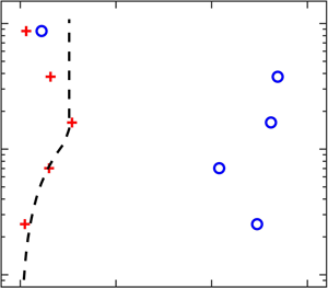For comparison, we also plot the classic estimate for the fluid momentum diffusivity in the log-law region, $\varepsilon _f = \kappa yu_\tau$ (Prandtl Reference Prandtl1952), and that for the defect layer ($y > 0.2\delta _{99}$), estimated as $\varepsilon _f = 0.09\delta _{99}u_\tau$ (Pope Reference Pope2000). In the log-law region, the turbulence causes the particles to disperse much faster in the streamwise direction, greatly exceeding the momentum diffusivity. This indicates that the effect of particle inertia (which increases particle dispersion) is dominating over the effect of gravitational drift (which reduces it), at least in what pertains streamwise dispersion. This agrees with theoretical arguments of Reeks (Reference Reeks1977) which predicted particles to disperse faster than tracers when the settling velocity $V_s < \langle u_f^{'2}\rangle ^{1/2}$, as it is the case here. Laboratory observations had confirmed this in homogeneous turbulence (Wells & Stock Reference Wells and Stock1983; Sabban & van Hout Reference Sabban and van Hout2011), and to our knowledge the present results are the first experimental observation of this effect in wall turbulence. On the other hand, $\varepsilon _{p,y}$ is equal to or smaller than the momentum diffusivity across the boundary layer, indicating that, in the vertical direction, the effect of gravity in decorrelating the particle motion slightly dominates.

Figure 17. Wall-normal profiles of streamwise and wall-normal diffusivity (blue circles and red crosses, respectively) compared to the theoretical profile of fluid momentum diffusivity (black dashed line).

3.6. Particle concentration and flux

Mean particle relative concentration as a function of wall-normal distance is plotted in figure 18. This is obtained by counting particles within logarithmically spaced wall-normal bins and normalizing by the mean concentration in the lowest bin, $C_0$. The observed power-law behaviour prompts a comparison with the concentration profile predicted by the theory of Rouse (Reference Rouse1937) and Prandtl (Reference Prandtl1952). This follows from the balance between gravitational settling and wall-normal turbulent flux

(3.5)\begin{equation} \langle C\rangle V_s - \varepsilon \frac{\partial\langle C\rangle}{\partial y} = \varPhi, \end{equation}

where $V_s$ is the particle settling velocity and $\varPhi$ is the net wall-normal flux of particles. Assuming equilibrium conditions ($\varPhi = 0$), the particles falling at $V_s = V_t$ and having the same diffusivity as the momentum in the turbulent boundary layer ($\varepsilon = \kappa yu_\tau$), leads to the well-known concentration profile (Prandtl Reference Prandtl1952)

(3.6)\begin{equation} \frac{\langle C\rangle}{\langle C\rangle_{ref}} = \left(\frac{y}{y_{ref}} \right)^{-{{\textit{Ro}}}} , \end{equation}

where the subscript denotes an arbitrary reference height and the corresponding concentration. Here, ${{\textit {Ro}}}=-V_t/(\kappa u_\tau )$ is the Rouse number, which quantifies the relative strength of gravitational settling and turbulent resuspension of the particles. Equation (3.6) is also plotted in figure 18 for comparison, which shows a much steeper drop in concentration with height than the measurements. A departure from Rouse–Prandtl theory is expected, notably because the latter does not account for particle inertia. In particular, Berk & Coletti (Reference Berk and Coletti2020) recently carried out a wind tunnel study of particle transport in turbulent boundary layers, and also reported a reduced slope of the concentration profile compared to the Rouse–Prandtl theory for a wide range of Stokes numbers. They hypothesized this to be due to a near-wall settling rate below the terminal velocity but could not accurately measure the particle vertical velocity. The present measurements corroborate their hypothesis (see figure 9b).

Figure 18. Wall-normal profile of mean particle concentration normalized by the concentration at the lowest wall-normal bin (black crosses). The power-law profile predicted by Rouse–Prandtl theory (red dashed line) is calculated from (3.6), where the arbitrary reference height is taken at $y_r^{+} = 90$.

The particle streamwise mass flux $Q_x$ is often of interest, especially in geophysical flows. Assuming advection dominates on the turbulent transport, the mean flux can be approximated from the mean concentration and mean velocity profiles, i.e. $\langle Q_x\rangle \approx \langle C\rangle \langle u_p\rangle$. Here, we compute the flux directly by counting particles crossing wall-normal planes, and verify that it does not vary with streamwise location within the imaging window, and that it is indistinguishable from the mean advective flux $\langle C\rangle \langle u_p\rangle$. The profile in figure 19, albeit with experimental scatter, suggests a power-law behaviour. In sediment transport and aeolian transport studies, the flux is often observed to decay exponentially with wall-normal height, thus identifying a characteristic length scale (e.g. Bagnold Reference Bagnold1941; Nishimura & Hunt Reference Nishimura and Hunt2000; Guala et al. Reference Guala, Manes, Clifton and Lehning2008; Kok et al. Reference Kok, Parteli, Michaels and Karam2012). However, those processes are inherently different from the present one: they are characterized by beds of particles mobilized by the impact of other particles, with their transport largely concentrated in a ‘saltation layer’. The present case instead is governed by suspension, and as such it does not possess a specific length scale beyond those associated with the fluid turbulence.

Figure 19. Wall-normal profile of particle streamwise mass flux normalized by the mass flux at the lowest wall-normal bin (black crosses), compared with a power-law fit (red dashed line).

3.7. Particle acceleration

The statistics of the particle acceleration provide insight not only on the kinematics but also on the forces at play. In figure 20(a) we present the profiles of mean and r.m.s. acceleration for both in-plane components. The mean acceleration profiles are in close agreement with the recent experiments of Ebrahimian et al. (Reference Ebrahimian, Sanders and Ghaemi2019), who considered particles with ${{\textit {St}}}^{+} = 3.9$ and $D_p^{+} = 6.8$ in a channel flow at $Re_\tau = 410$. The mean acceleration is negligible in the free stream, as expected in a fully developed flow. The streamwise acceleration increases to a positive maximum at $y^{+} \sim 50$, and then rapidly decays to become negative near the wall. When expressed in wall units, the negative mean streamwise acceleration we observe near the wall is significantly smaller in magnitude compared with the experiments of Gerashchenko et al. (Reference Gerashchenko, Sharp, Neuscamman and Warhaft2008). These authors considered microscopic water droplets, and therefore the discrepancy is likely rooted in the larger size of our particles compared to the viscous length scale, and the consequent effect of forces other than drag and gravity (Maxey & Riley Reference Maxey and Riley1983). The difference could also be related to particle interactions with the wall (addressed in § 3.8), which were likely inconsequential for the statistics of Gerashchenko et al. (Reference Gerashchenko, Sharp, Neuscamman and Warhaft2008).

Figure 20. (a) Profiles of mean streamwise and wall-normal particle acceleration. (b) Profiles of mean streamwise and wall-normal particle acceleration conditioned on whether particles are ascending (filled symbols) or descending (open symbols).

The mean wall-normal acceleration shows a qualitatively opposite trend compared to the streamwise component. At first, this would appear consistent with sweep and ejection being at the root of the acceleration profiles: upward vertical fluid fluctuations lifting the particles away from the wall also tend to decelerate them in streamwise direction, and vice versa for downward fluctuations. This view, however, does not consider the fact that the mean velocity of the particles is downward: thus, negative wall-normal accelerations are mostly associated with a decrease in magnitude of the negative velocity, i.e. hindering of the settling. We shall come back to this point shortly, when considering the fluid events associated with these particle statistics.

In Gerashchenko et al. (Reference Gerashchenko, Sharp, Neuscamman and Warhaft2008) and Lavezzo et al. (Reference Lavezzo, Soldati, Gerashchenko, Warhaft and Collins2010) it was argued that the gravitational settling of particles through the shear flow plays a crucial role in determining the streamwise acceleration. To explore this issue, we condition again the statistics on ascending and descending particles (figure 20b). It becomes apparent that the regions of positive and negative streamwise acceleration can be attributed to the ascending and descending particles, respectively. This is in line with arguments presented by Gerashchenko et al. (Reference Gerashchenko, Sharp, Neuscamman and Warhaft2008) and Ebrahimian et al. (Reference Ebrahimian, Sanders and Ghaemi2019): particles that fall vertically find themselves surrounded by slower fluid, which decelerates them; and vice versa for particles moving vertically upward. The mean vertical acceleration is instead unaffected by conditioning on ascending/descending particles.

We present profiles of r.m.s. particle acceleration in figure 21. The streamwise component is quantitatively close to what is reported by Gerashchenko et al. (Reference Gerashchenko, Sharp, Neuscamman and Warhaft2008), Zamansky et al. (Reference Zamansky, Vinkovic and Gorokhovski2011) and Ebrahimian et al. (Reference Ebrahimian, Sanders and Ghaemi2019). The wall-normal component instead reaches a peak 30 %–60 % larger than in those studies, being comparable to the streamwise component. We believe this to be mainly caused by gravitational effects. Already Gerashchenko et al. (Reference Gerashchenko, Sharp, Neuscamman and Warhaft2008) found that the particle r.m.s. acceleration of inertial particles was larger than that of tracer particles, in contrast with known trends in homogeneous turbulence (Bec et al. Reference Bec, Biferale, Boffetta, Celani, Cencini, Lanotte, Musacchio and Toschi2006; Ayyalasomayajula et al. Reference Ayyalasomayajula, Gylfason, Collins, Bodenschatz and Warhaft2006). Our particles are more inertial than those considered by Gerashchenko et al. (Reference Gerashchenko, Sharp, Neuscamman and Warhaft2008) (who had maximum ${{\textit {St}}}^{+} = 5.3$) and have larger settling velocity ($V_t/u_\tau = 0.75$, versus $V_t/u_\tau = 0.38$ in that study). In laboratory experiments it is not possible to conclusively disentangle inertia from gravity to determine what drives the higher vertical r.m.s. acceleration, but we can find hints in previous numerical studies where gravity could be suppressed. Lavezzo et al. (Reference Lavezzo, Soldati, Gerashchenko, Warhaft and Collins2010) demonstrated that gravity was the cause of increased r.m.s. acceleration in streamwise direction. This appears to be the case also for the wall-normal component, enhanced because the falling particles encounter rapidly changing flow structures. In further support of this view, the zero-gravity simulations of Zamansky et al. (Reference Zamansky, Vinkovic and Gorokhovski2011) found a decrease of both components of r.m.s. acceleration with increasing ${{\textit {St}}}^{+}$, while the recent simulations of Lee & Lee (Reference Lee and Lee2019) that included gravity showed the opposite trend, in agreement with Gerashchenko et al. (Reference Gerashchenko, Sharp, Neuscamman and Warhaft2008). Taken together, the above indicates that it is gravitational drift that causes heavy particles to have large r.m.s. accelerations, in both streamwise and wall-normal directions.

Figure 21. Wall-normal profiles of streamwise (blue circles) and wall-normal (red crosses) particle r.m.s. acceleration.

The acceleration of fluid tracers and inertial particles in turbulence are known to be intermittent, with super-Gaussian probabilities of high-acceleration events that strongly depend on the particle inertia. When gravity is absent or has negligible influence, it is established that increasing Stokes number leads to reduced intermittency (Bec et al. Reference Bec, Biferale, Boffetta, Celani, Cencini, Lanotte, Musacchio and Toschi2006; Gerashchenko et al. Reference Gerashchenko, Sharp, Neuscamman and Warhaft2008; Zamansky et al. Reference Zamansky, Vinkovic and Gorokhovski2011). We present the PDF of streamwise and wall-normal accelerations in figure 22. We plot separately the distributions for particles below and above $y^{+} = 100$, which helps in better understanding the observed behaviour. The stretched exponential tails indicate significant intermittency, with relatively large probability of extreme events. This is, however, much stronger for the particles far from the wall than for those close to it: the flatness of the distributions for $y^{+} < 100$ and $y^{+} > 100$ is 5.5 and 20.5 for the streamwise component, and 6.4 and 10.4 for the wall-normal component, respectively. This is because the particles closer to the wall interact with turbulent eddies of smaller time scales, and therefore have an effectively larger Stokes number (see figure 4a), which in turn causes them to ‘filter out’ intense fluid flow events (Bec et al. Reference Bec, Biferale, Boffetta, Celani, Cencini, Lanotte, Musacchio and Toschi2006). The crossing-trajectory effect, on the other hand, is weaker for the near-wall particles, which have small mean vertical velocity (figure 9b). Combined with the results for the r.m.s. accelerations, these results underscore the competing influence of gravity and inertia: the first enhances the variance and intermittency of the particle accelerations, while the second damps them, the net result depending on the relative importance of both effects.

Figure 22. PDFs of streamwise (blue filled symbols) and wall-normal (red open symbols) particle acceleration conditioned on $y^{+} < 100$ (circles) and $y^{+} > 100$ (triangles). The PDFs for $y^{+} > 100$ are shifted upward by a factor of $10^{3}$ for clarity.

The particle trajectories are influenced not only by the instantaneous values of their accelerations, but also by their temporal coherence. This is explored by calculating the Lagrangian autocorrelation of streamwise particle accelerations, defined analogously to the velocity autocorrelations and presented in figure 23 for various wall distances. The wall-normal acceleration (not shown) follows similar trends, but less clearly so due to experimental uncertainty on measuring quantities of smaller magnitude. Close to the wall ($y^{+} \lesssim 100$), the acceleration has significant temporal coherence, with the autocorrelation showing e-folding time of the order of the response time of the particles, before decaying monotonically to zero. This suggests that near-wall particles move in and out of streamwise-coherent turbulent structures and behave as if responding to step changes in the surrounding fluid velocity. We will show in § 3.8 that this picture is consistent with the behaviour of the particles that directly interact with the wall. At larger heights, the temporal coherence is greatly reduced and the oscillations around zero suggest a quick alternation of positive and negative accelerations. This is likely caused by settling with significant speed (close to the particle terminal velocity for $y^{+} \gtrsim 100$, see figure 9b), which causes the particles to move in a less coherent fashion. This is in line with the above-mentioned drop in streamwise diffusivity with increasing distance from the wall (figure 17).

Figure 23. Lagrangian autocorrelation of streamwise particle acceleration for five wall-normal bins. The wall-normal locations listed in the legend correspond to the centre of each bin.

3.8. Particle–wall interactions

In order to analyse the direct interactions with the wall, we consider the trajectories of particles that come in contact with it. An example of one such trajectory is shown in figure 24. Actual physical contact cannot be ascertained by the present imaging, and a lubrication layer is possibly maintained during those events. Still, we will use the word ‘contact’ to indicate the instances with no measurable wall–particle separation. More precisely, considering the variance of the particle diameters and the uncertainty in locating both the particles and the wall, we record contact when particle centroids are within 1.3 mean particle radii from the wall, i.e. when their wall-normal height is $y^{+} \leqslant 10.4$. The results below are robust to small modifications of this threshold. We define ‘touch-down’ and ‘lift-off’ events when this threshold is crossed by particles approaching and leaving the wall, respectively. In figure 24, touch-down occurs at about $\tau ^{+} = 15$ and lift-off at about $\tau ^{+} = 40$; in between, the particle is considered to be in continued contact with the wall. Below we present results from averaging 241 trajectories leading to a touch-down and 151 trajectories following a lift-off.

Figure 24. An example of an interaction between a particle and the wall. The blue curve shows the wall-normal distance of the particle centroid vs. time, with error bars representing the uncertainty in particle position. The dashed line represents a height of one particle radius above the wall, with the grey shaded region indicating the uncertainty in the particle radius and the wall location.

First, particle–wall interactions are characterized in terms of duration of contact, $t_{wall}$. Figure 25 presents the PDF of $t_{wall}$ in viscous units, which is well described by an exponential distribution. This is reminiscent of the distribution of ‘waiting times’ between touch-down and lift-off of the particles mobilized by the flow over a sediment bed (Einstein Reference Einstein1950; Ancey et al. Reference Ancey, Böhm, Jodeau and Frey2006; Fan et al. Reference Fan, Singh, Guala, Foufoula-Georgiou and Wu2016). In the case of bedload transport, an exponential distribution follows from assuming that touch-down and lift-off are time- and space-invariant Markovian processes (Ancey et al. Reference Ancey, Böhm, Jodeau and Frey2006), i.e. independent events that are influenced only by the present and local state. Accordingly, waiting times have often been modelled as induced by a random (Poissonian) distribution of turbulent fluctuations having sufficient strength to mobilize the particles (e.g. Papanicolaou et al. Reference Papanicolaou, Diplas, Evaggelopoulos and Fotopoulos2002). There are obvious differences between bedload transport and the present case: most notably, our particles are never at rest, as the wall shear stress exerted by the flow is much larger than the critical value for mobilizing them (Shields Reference Shields1936). Still, our distribution of contact times suggests these can be modelled by a similar stochastic process driven by randomly occurring fluid flow events above a certain threshold. We note that Cameron, Nikora & Witz (Reference Cameron, Nikora and Witz2020) recently showed the importance of very-large-scale motions (non-random, spatially correlated turbulent events) for sediment entrainment. While this points to the limitations of considering turbulent fluctuations to be random, their study was conducted at much higher Reynolds numbers for which very-large-scale motions are more prominent than in our case (Smits, McKeon & Marusic Reference Smits, McKeon and Marusic2011).

Figure 25. PDF of duration of particle–wall interactions, defined as the length of time particles spend continuously within 1.3 mean particle radii of the wall.

The exponential distribution of $t_{wall}$ suggests a characteristic time $\tau _{wall}$, such that its duration probability can be approximated as $\mathrm {PDF}(t_{wall}) \propto \exp ({-t_{wall}}/{\tau _{wall}} )$. A least-squares fit returns $\tau _{wall} = 13.5\tau ^{+}$, which is remarkably close to the particle response time $\tau _p/\tau ^{+} = {{\textit {St}}}^{+} = 15$. This suggests that both particle inertia and the fluid fluctuations play a role in determining the duration of the wall contact, and one may hypothesize a scaling $\tau _{wall}^{+} \sim {{\textit {St}}}^{+}$. This is indeed consistent with the results reported by Ebrahimian et al. (Reference Ebrahimian, Sanders and Ghaemi2019), whose particles had ${{\textit {St}}}^{+} = 3.9$ and a mean wall contact time around $4\tau ^{+}$. Because that is the only previous study reporting contact times for suspended particles, further research is warranted to corroborate this ansatz. We note that, in sediment transport, the waiting time was originally suggested by Einstein (Reference Einstein1950) to be inversely proportional to the particle settling velocity, but it was later recognized that an inverse proportionality with fluid velocity showed better agreement with observations, and with the view that the particle entrainment rate depends on the strength of the turbulent fluctuations (Ancey et al. Reference Ancey, Böhm, Jodeau and Frey2006, Reference Ancey, Davison, Böhm, Jodeau and Frey2008).

As the particles are never at rest, one may consider the possibility that the short contact times are associated with a rebound process. However, even assuming an incident velocity $V_i$ equal to the maximum vertical velocity in the $20\tau ^{+}$ preceding touch-down (see below), the impact Stokes number $\rho _pV_iD_p/(9\mu )$ is of order unity – well below the threshold for a non-zero restitution coefficient (Joseph et al. Reference Joseph, Zenit, Hunt and Rosenwinkel2001; Gondret, Lance & Petit Reference Gondret, Lance and Petit2002). Thus, in the present regime, the kinetic energy of the particle associated with its wall-normal motion is expected to be dissipated at contact, with no effective rebound.

The particle–wall interactions can also be characterized by the angle $\theta _p$ of near-wall particle trajectories as they approach or recede from the wall. The trajectory angle is defined as $\theta _p = \mathrm {atan}(v_p/u_p)$, such that $\theta _p$ is negative for particles approaching the wall and positive for particles receding from it. The set of particles within one particle diameter of the wall ($y^{+} < 16$) is considered. The PDF of $\theta _p$ is shown in figure 26; it displays stretched tails (with a flatness of 6.7), and measurable preference for positive values (with a skewness of 0.65). The distribution of angles is narrower than what reported by Ebrahimian et al. (Reference Ebrahimian, Sanders and Ghaemi2019). This is attributed to the larger inertia of the present particles (${{\textit {St}}}^{+} = 15$ versus 3.9), resulting in a slower response time to fluid velocity fluctuations and thus shallower near-wall trajectory angles. The positive skewness indicates that, despite gravity, relatively sharp lift-offs may occur.

Figure 26. PDF of the angle of trajectories for near-wall ($y^{+} < D_p^{+}$) particles.

The mechanisms behind particle touch-down and lift-off can be further understood by considering the Lagrangian averages along the particle trajectories. To this end, we first identify the moments of touch-down and lift-off (within the temporal resolution of $1/500\ \textrm {s} = 0.7\tau ^{+}$), and then average over all trajectories leading to and following those events, respectively. Figure 27 displays the average particle wall-normal distance, streamwise velocity and vertical velocity during the $20\tau ^{+}$ before touch-down and after lift-off. We do not report Lagrangian statistics during particle–wall contact, as the range of contact durations thwarts a consistent averaging process. However, we note that the wall-normal positions, velocities and accelerations at touch-down are very close to those at lift-off.

Figure 27. Lagrangian means of particle wall-normal coordinate (a,b), streamwise velocity (c,d) and wall-normal velocity (e,f) averaged over all identified touch-down events (a,c,e) and lift-off events (b,d,f). The time axis shows the time interval before or after lift-off or touch-down, respectively, and ${\rm \Delta} t^{+} = 0$ represents the moment of lift-off or touch-down.

The Lagrangian averages of the wall-normal distance indicate that the particles descending to the wall follow a somewhat steeper trajectory than those ascending from it (figures 27a and 27b). This is confirmed by the plots of the vertical velocities (figures 27e and 27f) and is due to a combination of gravity and Saffman lift (which is directed downward, as demonstrated below). The streamwise velocity declines before touch-down (figure 27c), because the particles approaching the wall are surrounded by slower and slower fluid, which applies on them drag in the negative $x$-direction. After lift-off, although the particles ascend at a similar pace as they descended, they regain streamwise velocity much more slowly (figure 27d). This fits the view of particles being lifted from the wall by ejections, i.e. events with smaller streamwise fluid momentum compared to the local mean.

The Lagrangian average of the fluid velocity experienced by the particles along their trajectory helps in the interpretation of the above trends. Figures 28(a) and 28(b) show that, before and after wall contact, the streamwise velocity of the fluid surrounding the particles is significantly lower than the local particle velocity (see figures 27c and 27d). (This is not captured by the unconditioned mean profiles presented §§ 3.1 and 3.2. We remark that the particles coming in contact with the wall are a small fraction of the total in the corresponding bin.) The direction of the streamwise slip velocity implies that, close to wall contact, drag acts against the direction of motion and Saffman lift is directed downward (in consideration of the slip velocity and the fluid velocity gradient, Saffman Reference Saffman1965). The streamwise fluid velocity along the trajectory is also significantly lower than the local mean fluid velocity (assuming a canonical boundary-layer profile, see figure 7); therefore, the particles are in regions of negative streamwise fluctuations. Because the vertical fluid velocity is negative before touch-down (figure 28c) and positive after lift-off (figure 28d), particles approaching and leaving the wall experience Q3 events and Q2 events, respectively. This confirms once more that ejections (in Q2) are critical to lift particles from the wall, while the role of sweeps (in Q4) is not dominant near wall contact. Importantly, figure 28(d) indicates that the vertical fluid velocity becomes positive just as the particles leave the wall: that is, lift-off happens when the particle starts to experience a fluid ejection. This is in line with the view that the duration of the contact time is dictated by the occurring of turbulent events.

Figure 28. Lagrangian means of streamwise (a,b) and wall-normal (c,d) fluid velocity at particle location averaged over all identified touch-down events (a,c) and lift-off events (b,d). The time axis shows the time interval before or after lift-off or touch-down, respectively, and ${\rm \Delta} t^{+} = 0$ represents the moment of lift-off or touch-down.

A material frame of reference attached to the particles is the most appropriate to investigate the forces acting on them, and thus we now consider the accelerations tangential and normal to the local trajectory, $a_{t,p}$ and $a_{n,p}$, respectively

(3.7)\begin{gather} a_{t,p} = a_{x,p}\cos (\theta_p) + a_{y,p}\sin (\theta_p) \end{gather}

(3.8)\begin{gather}a_{n,p} = a_{y,p}\cos (\theta_p) - a_{x,p}\sin (\theta_p). \end{gather}

Note that since $\theta _p$ is relatively small, the tangential and normal accelerations are very similar in magnitude to the horizontal and vertical components, respectively. We can make inferences on the role and respective importance of drag, gravity and Saffman lift. Other forces are expected to be important as well, such as added mass, fluid acceleration, Basset history and Faxén corrections and rotation-induced (Magnus) lift (Maxey & Riley Reference Maxey and Riley1983; Crowe et al. Reference Crowe, Schwarzkopf, Sommerfeld and Tsuji2011; Mathai et al. Reference Mathai, Loeffen, Chan and Wildeman2019); however, it is not trivial to infer their behaviour from experimental data, so our qualitative considerations will not focus on these forces.

The Lagrangian averages of the accelerations before and after wall contact are plotted in figure 29. As the particles approach the wall before touch-down, they experience increasingly negative tangential acceleration (figure 29a), reflecting the drag force opposing their motion. Notice that, while we are outside the assumptions of viscous steady flow made to derive analytical results, we expect the wall proximity to enhance drag for a particle moving parallel to a solid boundary (Brenner Reference Brenner1965). The negative streamwise acceleration peaks around $5\tau ^{+}$ before touch-down and then decreases in magnitude. This is possibly due to lubrication effects, as the average particle is then only a fraction of its diameter away from the wall. Higher resolution measurements are needed to draw firm conclusions in this regard.

Figure 29. Lagrangian means of particle tangential acceleration (a,b) and normal acceleration (c,d) averaged over all identified touch-down events (a,c) and lift-off events (b,d). The time axis shows the time interval before or after lift-off or touch-down, respectively, and ${\rm \Delta} t^{+} = 0$ represents the moment of lift-off or touch-down.

As the particles leave the wall and reach faster fluid layers, they at first experience negative streamwise acceleration, but this shrinks in magnitude and eventually reaches a small positive plateau (figure 29b). This follows from the particles being entrained into faster fluid strata, which reduces the negative drag. However, because the particles are still faster than the surrounding fluid (see figures 27d and 28b), the drag is expected to remain negative. Thus, the positive streamwise acceleration must be a consequence of other forces. Added mass and fluid acceleration force are prime candidates, because the acceleration of the fluid along the particle trajectory is positive and larger than that of the particle (compare again figures 27d and 28b). Further studies to quantify these forces are warranted.

The normal acceleration becomes positive before touch-down (figure 29c) since the downward particle velocity is decreasing in magnitude as the wall is approached. This is qualitatively consistent with the increase in drag predicted in viscous flows when a particle travels towards a wall (Brenner Reference Brenner1965). The interaction with a lubrication layer may also contribute to slowing down the descent. The downward-directed Saffman lift increases the magnitude of the downward particle velocity before touch-down and decreases the magnitude of the upward velocity after lift-off. Thus, Saffman lift (along with gravity) is the likely cause of the drop in positive normal acceleration after the particles has left the wall (figure 29d). Simulations of Lee & Balachandar (Reference Lee and Balachandar2010) suggested the Magnus force to be relatively small, but the estimates of Ebrahimian et al. (Reference Ebrahimian, Sanders and Ghaemi2019) suggested it could be sufficient to overcome gravity. Here, the magnitude of the Magnus force cannot be estimated without knowing whether the particles are actually in contact with the wall, as this would dictate their rolling motion.