2.1. Flow facility for an upward jet with a crossflow

The experiments were conducted in a wind tunnel ($2075\ \textrm {mm}\times 600\ \textrm {mm}\times 800\ \textrm {mm}$ in the horizontal ($x$), transverse ($y$) and vertical ($z$) directions, respectively), as shown in figure 2(a). The test section was made of $10$ mm thick transparent acrylic plates. At the exit of the test section, a high-efficiency particulate air filter was installed to filter out particles (or seeders for particle image velocimetry), and to prevent flow distortions owing to backflow. From a nozzle exit at the bottom, the upward jet (the bulk velocity varied as $U_{j} = 1.0\text {--}3.5\ \textrm {m}\ \textrm {s}^{-1}$) was ejected through a long stainless steel square pipe with a length ($L$) and side length ($D$) of 400 and $22.5$ mm, respectively (the aspect ratio of which is large enough to have a fully developed flow at the exit). The Reynolds number of the vertical jet with crossflow was $Re_{D} = \bar {u}_{m}D/\nu = 1170\text {--}5200$, where $\bar {u}_{m}$ is the time-averaged maximum air velocity measured directly above the exit and $\nu$ is the kinematic viscosity of air. Throughout this paper, an upper bar denotes the time-averaged value. To ensure the uniformity of the jet and crossflow, a stainless mesh screen (wire diameter and opening size of $0.5$ mm and $2.67$ mm, respectively) was installed at the exits. The pipe was spaced $300$ mm apart from the side walls of the test section. Considering the spreading rate of the jet at a similar $Re_D$, it was assumed that the jet was not affected by the interference of the side wall (Kwon & Seo Reference Kwon and Seo2005; Fellouah, Ball & Pollard Reference Fellouah, Ball and Pollard2009). The horizontal crossflow was blown through a rectangular duct toward the vertical jet, generated by a brushless DC blower fan ($\text {maximum air volume} = 7.7\ \textrm {m}^{3}\ \min ^{-1}$) installed near the test section floor. The velocity profiles measured at the exit of the vertical jet (at $z/D = 0$) and horizontal crossflow (at $x/D = -13.3$) are shown in figure 2(b). As shown, the crossflow is approximately symmetric and has a velocity peak at $z/D \simeq 2.0$. Jet exit fluid velocity exhibits the common feature of a parabolic profile (Mi, Nobes & Nathan Reference Mi, Nobes and Nathan2001; Zhang et al. Reference Zhang, Xu, Pollard and Mi2013; Lau & Nathan Reference Lau and Nathan2014, Reference Lau and Nathan2016). For the particle velocity at the jet exit, the profile with $St \ll 1.0$ follows the fluid velocity, and the gravity effect increases as $St$ becomes higher (particles tend to fall down near the edge of the exit). It should be noted that the crossflow did not fully cover the cross-sectional area of the test section; rather, the fan outlet size was $-3.7 \leqslant y/D \leqslant 3.7$ and $0 \leqslant z/D \leqslant 2.93$, indicating that the crossflow partially covered the $y$–$z$ plane of the test section. This is a specific condition but we intended to mimic the wind blowing along a locally confined area near the particle source (much closer to situations found in nature and industrial sites, which are normally non-uniform) and it is more suitable to investigate particle dispersion in terms of the interaction with the vortical structure of which the coherency varies spatially. The bulk velocity of the crossflow ($U_c$) varied up to $3.0\ \textrm {m}\ \textrm {s}^{-1}$; thus, the ranges of the velocity ratio were $R = U_{j}/U_{c} = 1.0\text {--}1.2$, 3.0–3.5 and $\infty$.

Figure 2. (a) Experimental set-up for measuring the continuous-phase (air) flow structure and dispersed solid particle concentration in $x$–$z$ and $x$–$y$ planes with a particle image velocimetry and high-speed imaging (camera and lasers are shown for $x$–$z$ plane measurement). (b) Time-averaged velocity profiles for the crossflow and vertical jet measured at the exit of the crossflow duct ($x/D = -13.3$) and jet pipe ($z/D = 0$), respectively: $\bullet$, gas velocity; $\blacksquare$, red, particle velocity ($St = 0.013$); $\blacksquare$, light pink, particle velocity ($St = 1.07$); $\square$, particle velocity ($St = 15.71$).

2.2. Description of the solid particles

Considering the properties (density, chemical compositions and so on) of fine dust pollutants commonly found in nature (Li et al. Reference Li, Shao, Wang, Shen, Yang and Tang2010; Hu et al. Reference Hu, Peng, Sun, Yue, Guo, Wiedensohler and Wu2012), we consider $99.9\,\%$ silicon spherical particles (density $\rho _{p} = 2.33\ \textrm {g}\ \textrm {cm}^{-3}$) as the dispersed phase. These were loaded in the vertical jet using an in-house fluidized-bed type seeding device (figure 2a). As shown in figure 3, the mean particle diameter ($\bar {d}_{p}$) was varied as $6$, $53.6$ and $205.5\ \mathrm {\mu }\textrm {m}$, respectively, and the particle size followed a Gaussian distribution with a standard deviation around $15\,\%$. The particle size distribution was measured using a particle size analyser (Mastersizer 2000, Marvern Panalytical Ltd.) in a 10 gram sample per each group of size. This apparatus uses a laser diffraction technique based on the principles of static light and Mie scattering theory; smaller (larger) particles scatter the light at larger (smaller) angles. With this range of particle size distribution (figure 3), the range of Stokes number does not change significantly in orders. Therefore, in the same group of particle size, it is expected that the specific particle dynamics under the interaction with the flow is retained. In addition, previous studies also used particles with a comparable level (9–17 %) of standard deviation in size (Anderson & Longmire Reference Anderson and Longmire1995; Hwang & Eaton Reference Hwang and Eaton2006; Dou et al. Reference Dou, Bragg, Hammond, Liang, Collins and Meng2018). The modulation of the continuous-phase flow turbulence owing to the interaction with the dispersed phase is also an important issue in a multiphase flow (Hwang & Eaton Reference Hwang and Eaton2006; Abdelsamie & Lee Reference Abdelsamie and Lee2012; Kim, Lee & Park Reference Kim, Lee and Park2016; Lee & Park Reference Lee and Park2020), but this was not the point of this study. Thus, we focused on the particle behaviours owing to the background flow (i.e. one-way coupling). The particle volume fraction ($\phi = \text {total}$ solid particle volume/test section volume) was determined as approximately $2 \times 10^{-7}$ ($0.3\ ({\pm }0.03$) gram of particles were used per each trial of measurement); this was sufficiently low to assume that the effects of the particles on the air flow and particle-to-particle collisions were negligible (Elghobashi Reference Elghobashi2006).

Figure 3. Probability density function (p.d.f.) of particle size considered in the present study.

To characterize the dynamics of the particles, we considered the particle Stokes number, $St = \tau _{p}/\tau _{f}$. The flow time scale was defined as $\tau _{f}=D/\bar {u}_{m}$, and the particle relaxation time scale was the ratio of particle settling velocity ($V_s$) to gravitational acceleration ($g$). A similar definition of flow time scale based on the bulk flow scale was also adopted for investigating the larger-scale particle dispersion (Fessler & Eaton Reference Fessler and Eaton1997; Lau & Nathan Reference Lau and Nathan2014, Reference Lau and Nathan2016). The slip velocity $(v-u)$ of the particle tends to saturate to a settling velocity as the drag force ($F_D$) is balanced with the gravitational force ($F_G$). Here, $u$ and $v$ is the velocity of air flow and particle, respectively. Given a single rigid particle released in stagnant air, the equation for particle motion for balanced state is defined as $m_{p}(\textrm {d}v/\textrm {d}t)=F_{G}-F_{D}=1/6(\rho _{p}-\rho _{g}){\rm \pi} \bar {d}_{p}^{3}g-F_{D}=0$, where $m_p$ is the mass of a particle, $\rho _p$ and $\rho _g$ are the density of the particle and gas (air), respectively. The drag force depends on the particle Reynolds number ($Re_p$), which is based on the slip velocity, i.e. $Re_{p}=\rho _{p}\bar {d}_{p}|v-u|/\mu$ ($\mu$: dynamic viscosity of air) (see table 1). When $Re_{p} < 1$, which applies to most of the present cases, the viscous effect is much stronger than the inertia, and the Stokes’ drag holds as $F_{D} = 3{\rm \pi} \mu (v-u)\bar {d}_{p}$. As $Re_p$ increases over $1.0$, the drag force transitions to be proportional to the square of the slip velocity, as $F_{D} = C_{D}({\rm \pi} /8) \rho _g\bar {d}_{p}^{2}(v-u)^{2}$. We used $C_{D}=(24/Re_{p})\cdot (1+0.15Re_{p}^{0.687})$ for the drag coefficient, which has been validated for $1 < Re_{p} < 800$ (Schiller & Neumann Reference Schiller and Neumann1933). For the present lower $\phi$, the particle–particle interactions were negligible, and the above relation for a single-particle was used without modification (Fessler & Eaton Reference Fessler and Eaton1997; Lau & Nathan Reference Lau and Nathan2016). Therefore, the Stokes number was calculated as

(2.1)\begin{equation} St=\frac{\tau_{p}}{\tau_{f}}= \left\{ \begin{array}{@{}ll} \sqrt{\dfrac{4\rho_{p}\bar{d}_{p}}{3\rho_{g}C_{D}g}} \dfrac{\bar{u}_{m}}{D} & \mbox{for}\ 1 < Re_{p} < 800, \\ \dfrac{\rho_{p}\bar{d}_{p}^{2}}{18\mu} \dfrac{\bar{u}_{m}}{D} & \mbox{for}\ Re_{p} \leqslant 1. \end{array}\right. \end{equation}

As shown, the gravitational effect is additionally included for cases with higher $Re_{p}$. Based on varying the jet velocity and particle size together, the present experiments were performed in the range of $St = 0.01\text {--}27.42$. The detailed flow variables considered in the present study are listed in table 1.

Table 1. Summary of the considered experimental parameters of gas and solid phases.

2.3. Velocity measurement of the solid and gas phases

In the present configuration it was not possible to distinguish the silicon particles and seeders for particle image velocimetry (PIV) in the optically obtained images for the velocity measurements. Thus, the velocity fields of the solid particles and background flow were measured separately. This approach was acceptable as the solid–gas flow belonged to a one-way coupling regime (Fessler & Eaton Reference Fessler and Eaton1997; Fu, Wang & Gu Reference Fu, Wang and Gu2013), and the same vortex structures as those measured in a single-phase flow determine the particle motion in the two-phase flow. For the PIV of the air flow, high-purity liquid polyol (fog fluid standard, Dantec Dynamics) was atomized into oil droplets (nominal diameter of $1\ \mathrm {\mu }\textrm {m}$) by smoke generators (Safex, Dantec Dynamics), and was fed into both the vertical jet and crossflow openings as tracers (figure 2a). As a light source, a $5$ W continuous wave (CW) laser (RayPower 5000, Dantec Dynamics) with a wavelength of 532 nm was used to illuminate the measurement plane. To measure the velocity of the solid particles, we used the same set-up, except for employing silicon particles instead of the seeders for the PIV. A particle tracking method (PTV) would be more adequate to measure the velocity of individual particles; however, it is quite difficult to apply if the size of the particle is much smaller than the pixel size and the solid fraction is high, like the present study. Poelma, Westerweel & Ooms (Reference Poelma, Westerweel and Ooms2007) explained that less than $100$ particles in an image is suitable to apply PTV; which is not satisfied in the present study. When the PTV is not feasible, a PIV has been commonly used to measure the solid particle velocity in investigating the particle-laden flows (Anderson & Longmire Reference Anderson and Longmire1995; Tóth, Anthoine & Riethmuller Reference Tóth, Anthoine and Riethmuller2009; Lau & Nathan Reference Lau and Nathan2014, Reference Lau and Nathan2016; Liu et al. Reference Liu, Jiang, Zhang and Li2016). A high-speed camera (SpeedSense M310, Dantec Dynamics) equipped with a 50 mm lens (Nikon) was used to capture raw images at a speed of 3200 frames per second. The measurements of the velocities and particle distributions (see § 2.4) were performed at the same locations. For the three-dimensional analysis, we perform the measurements on multiple $x$–$z$ (side view; at $y/D = 0$, $0.5$, $1.0$ and $2.0$) and $x$–$y$ (top view; at $z/D = 0.5$, $1.0$, $2.0$, $5.0$ and $10.0$) planes. For the $x$–$z$ plane measurement, the size of the field of view (FoV) was $-4.0 \leqslant x/D \leqslant 4.0$ and $-0.6 \leqslant z/D \leqslant 34.0$ for the cases without crossflow, and $-2.3 \leqslant x/D \leqslant 15.0$ and $-0.7 \leqslant z/D \leqslant 11.0$ for the cases with crossflow. To cover the large side view FoV in the case without crossflow, the FoV was divided into three segments and measured. For the $x$–$y$ plane measurement, the FoV size is $-5.0 \leqslant x/D \leqslant 10.5$, and $-7.0 \leqslant y/D \leqslant 7.0$. The spatial resolution of the velocity measurement was $0.01D-0.014D$ or $37.5\bar {d}_{p}-52.5\bar {d}_{p}$, based on the smallest solid particle ($\bar {d}_{p} = 6\ \mathrm {\mu }\textrm {m}$). As we did not focus on particle gathering in the turbulence scales, this was considered sufficient for understanding the vortex-induced particle dispersion. A cross-correlation algorithm based on a fast Fourier transform was used to evaluate the velocity vectors for each pair of tracer (or particle) images, with an interrogation window (IW) of $32 \times 32$ pixels ($50\,\%$ overlap). Spurious vectors were detected by the normalized median test (Westerweel & Scarano Reference Westerweel and Scarano2005), and were replaced with the average of the surrounding vectors in a $3 \times 3$ grid.

Experimental uncertainties in velocity measurement are caused by various sources (Raffel, Willert & Kompenhans Reference Raffel, Willert and Kompenhans2007). When the velocity evaluated using the PIV technique is expressed in relation to $M$ (magnification factor), $\Delta t$ (time interval between successive images) and $\Delta s$ (particle displacement during $\Delta t$), the uncertainty in the measured velocity can be estimated as $\delta (u)=\sqrt {(\delta (M)^{2} + \delta (\Delta t)^{2} + \delta (\Delta s)^{2}}$; percentage errors ($\delta$) in obtaining each variable are combined (Lawson et al. Reference Lawson, Rudman, Guerra and Liow1999; Kim, Kim & Park Reference Kim, Kim and Park2015; Choi & Park Reference Choi and Park2018). During the calibration, we used a two-dimensional calibration target, and $\delta (M)$ was found to be approximately 0.3–0.4 %, with $M = 266\text {--}499\ \mathrm {\mu }\textrm {m}\ \textrm {pixel}^{-1}$. For the time separation, the inter-fame time was 500 ns, and the corresponding $\delta (\Delta t)$ was $0.15\,\%$. Finally, as affected by the pixel resolution of $0.1$ pixels, $\delta (\Delta s)$ was estimated to be approximately $0.7\,\%$ for $\Delta s = 6.6$ pixel. Therefore, the overall uncertainty in the measured velocity was approximately $1.0\,\%$.

2.4. Measurement of particle concentration

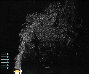
The particle concentration was quantified based on the light intensity of the Mie scattering signal from the solid particles, which is proportional to the particle number density. This is known as planar nephelometry (PN) (Birzer, Kalt & Nathan Reference Birzer, Kalt and Nathan2012; Lau & Nathan Reference Lau and Nathan2014). We used a planar laser sheet, the same as that used in the PIV, as a light source. The relative light intensity (proportional to the particle concentration) shows up as a different grey-scale level of each pixel in the images; these are thus quantified as indexes for relative particle concentrations in post-processing for noise removal (Birzer et al. Reference Birzer, Kalt and Nathan2012), as shown in figure 4(a). First, the grey-level in each pixel was calculated and normalized in a range of $0$ (black) to $1.0$ (white). Considering that the grey-level (light intensity) represents the relative particle concentration, we subtracted the grey-level distribution of the background image (taken at the same condition except for the particles) from that of the raw images, for the purpose of noise removal (typically, the normalized grey-level values below $0.1$). Then, the concentration ($\varTheta$) per IW was evaluated as an area fraction, where $\varTheta = (\text {sum of the grey-level values contained in IW})/(\text {IW area})$ (figure 4a). Here, the size of the IW ($32 \times 32$ pixels) was the same as that of the PIV measurement. Meanwhile, when measuring the cases without crossflow on the $x$–$z$ planes, two CW lasers were arranged vertically to minimize the effects of non-uniform illumination owing to the large FoV (figure 2a). By using two lasers, we found that the low-light-intensity region at the edges of the laser sheet could be compensated for, and a full illumination on the entire FoV was achieved.

Figure 4. Particle concentration measurement by PN: (a) raw image of solid particles and a schematic diagram to calculate light intensity of an IW (yellow colour: pixels identified as being occupied by solid particles; grey colour: noise); (b) correction of non-uniform laser light sheet; (c) correction of measured particle concentration.

As we optically measured the particle concentration based on light scattering in a relatively large FoV, the spatial non-uniformity of the incident laser power could affect the results (Kalt & Nathan Reference Kalt and Nathan2007). When the particle volume fraction is smaller than ${\sim } 10^{-5}$ ($2 \times 10^{-7}$ for the present cases), the attenuation of light power owing to particle shadows is known to be negligible (Kalt, Birzer & Nathan Reference Kalt, Birzer and Nathan2007; Cheong, Birzer & Lau Reference Cheong, Birzer and Lau2016). However, we attempted to compensate for the possible distortions owing to particles and the quality of the laser sheet. As a first step, we measured the level of light attenuation along the beam direction, and the effect of the laser sheet profile. We introduced uniformly distributed oil droplets into the FoV, and measured the reflected light intensity (i.e. the grey-level). As the smoke was distributed uniformly, this provided us with information on the power intensity irregularity in the laser sheet. Based on the measured oil droplet field image, we determined the correction constant ($C^{*}$) per IW; $C^{*}$ was defined as $C^{*}(i, j) = 1.0 + S_{md} - S_{laser}(i, j)$, where $S_{laser}$ is the laser light intensity value of each IW and $S_{md}$ is the median value of $S_{laser}$. Here $S_{laser}$ was calculated by the same method to obtain $\varTheta$, and was normalized by its own maximum value in the FoV. In this study, $(i, j)$ represented the coordinates of the IW. As shown in figure 4(b), the correction factor was higher near the laser outlet and lower at the edge of the laser sheet. Using this map of $C^{*}$, the measured raw values (concentration) were calibrated; biased concentration values at positions with higher (lower) power intensity than $S_{md}$ were corrected. Once the correction factor was obtained, it is multiplied by the raw particle concentration ($\varTheta$) values in each IW, and the corrected concentration ($\varTheta _{c}$) was obtained as $\varTheta _{c}(i, j) = \varTheta (i, j)\cdot C^{*}(i, j)$. An example is shown in figure 4(c). Together with previous studies (Kalt & Nathan Reference Kalt and Nathan2007), this correction procedure prevented excessive data distortion in locations where the laser power intensity was drastically biased.

For the corrected (calibrated) raw images, we evaluated the particle concentration distribution, which was further normalized ($\hat {\varTheta } = \bar {\varTheta }_{c}/\bar {\varTheta }_{b}$) by the bulk concentration ($\bar {\varTheta }_{b}$), defined as follows (Lau & Nathan Reference Lau and Nathan2014):

(2.2)\begin{equation} \bar{\varTheta}_{b} = \frac{1}{D^{2}V_{j}}\int^{D/2}_{{-}D/2}\int^{D/2}_{{-}D/2}\bar{\varTheta}_{exit}(x, y)\bar{v}_{exit}(x, y)\,\textrm{d}x\,\textrm{d}y. \end{equation}

Here, $\bar {\varTheta }_{exit}$ and $\bar {v}_{exit}$ are the time-averaged local concentration and velocity of the particles, respectively, and $V_{j}$ is the bulk particle (solid-phase) velocity, measured at the jet exit ($z/D = 0$).

4.1. Decay of particle concentration away from jet exit (particle source)

In this section we evaluate the characteristics of the three-dimensional particle dispersion depending on $R$ and $St$. Figure 12 shows typical instantaneous particle distributions (raw images) for selected cases of lower $R$ (${\sim }1.0$) and higher $R$ $({\sim }3.0)$ values, in which the CVP is generated in the flow (figures 7, 10 and 11). The most prominent feature in this figure is the distinguishable difference in the particle distribution characteristics near the jet exit ($z/D = 0.5$) with $R$. When $R \sim 1.0$, the solid particles of $St = 0.01$ and $0.965$ are dispersed by the coherent vortex structure near the jet exit, but the detailed pattern is different (figure 12a). When $St \lesssim 1.0$, we observe a $C$-shaped particle cluster whose leading edge is located at the jet exit, owing to a strong CVP. As the jet develops, the particles with $St \ll 1.0$ are transported along not only the transverse ($y$) direction, but also the crossflow-streamwise ($x$) direction at $z/D = 2.0$, where the CVP starts to collapse. Nevertheless, a large number of particles still gather at the leading edge of the $C$-shaped cluster when the Stokes number is close to $1.0$. When $St \gg 1.0$, the particles tend to spread independently of the vortex structure; they are clustered only above the jet exit and disperse uniformly along the streamwise and transverse directions.

Figure 12. Raw images measured for the solid particle dispersion on $x$–$y$ planes for selected cases with crossflow: (a) $R \sim 1.0$. (b) $R \sim 3.0$.

On the other hand, for higher $R$ cases (${\sim }3.0$), most of the particles are detected on the jet exit, as the particle movement is less affected by the CVP (figure 12b). Rather, after the CVP collapses, a relatively vague $C$-shaped particle cluster is observed for $St \lesssim 1.0$ away from the exit ($z/D$ value of ${\sim }5.0$). Unlike the lower $R$ cases (figure 12a), the particles gather at the leading edge of the $C$-shaped cluster, even at $St \ll 1.0$. For $St \gg 1.0$, the particles move independently of the vortex structures, and tend to spread in the transverse direction above the jet exit. As shown in this representative data, it is clear that the responses of the particles to the coherent vortex structure change mainly according to $St$ as the velocity ratio decreases. As discussed in § 3, the vertical jet (without crossflow) does not change substantially with $Re_D$. With crossflow, the global pictures of the vortical structures are not affected drastically by $Re_D$, but it needs to be considered when the crossflow is weak (higher $R$ cases). The effect of $Re_D$ (inertia) on the particle dispersion (if any) is reflected in $St$.

To quantitatively analyse the particle dispersion, the radial ($r/D$) distribution of the particle concentration is evaluated for the time-averaged solid-phase fields on each of the four $x$–$z$ planes ($y/D = 0$, $0.5$, $1.0$ and $2.0$). The corrected local concentration values are normalized by the bulk concentration as $\hat {\varTheta } = \bar {\varTheta }_{c}/\bar {\varTheta }_{b}$ (see § 2.4). Figure 13 shows the concentration distributions for selected cases, and the data in each $x$–$z$ plane are distinguished with different colours. In figure 13 the border of the data indicates the maximum concentration ($\hat {\varTheta }_{m}$), as measured at the radial distance from the jet exit (particle source). For all cases, it is found that the maximum value begins to decrease steeply from the particle source ($r/D = 0$); subsequently, the decay rate becomes quite slow away from the origin. We define the location at which the decaying rate changes as a division point ($P_d$). To determine $P_d$ consistently, forward (FD) and backward (BD) differentials of the maximum concentration are calculated as $\textrm {FD}_{i}=(\hat {\varTheta }_{m,N}-\hat {\varTheta }_{m,i})/((r/D)_{N}-(r/D)_{i})$ and $\textrm {BD}_i=(\hat {\varTheta }_{m,i}-\hat {\varTheta }_{m,1})/((r/D)_{i}-(r/D)_{1})$, where $i = 1,\ldots , N$ ($N$: last position with the data of $\hat {\varTheta }$). The position of the maximum BD is designated as $P_d$. The values of BD and FD at the position of $P_d$ are referred to as $G_1$ and $G_2$, respectively, indicating a representative decaying rate in each realm. As noted in figure 13, the position of $P_d$ moves toward the source as $R$ decreases. Accordingly, without crossflow, $P_d$ appears at $r/D > 20.0$, with a slower decaying slope (figure 13a); however, with crossflow, the particle concentration decreases at a faster rate, and the position of $P_d$ occurs at $r/D < 10.0$ (figure 13b,c). On the other hand, the trend of the concentration peak (distribution) changes across the plane of $y/D = 1.0$, and we think this is because the $y/D = 1.0$ plane corresponds to the edge of coherent vortical structures; jet shear-layer vortex and CVP for the cases without and with crossflow, respectively (figures 6 and 7).

Figure 13. The normalized particle concentration ($\hat {\varTheta }$) on $x$–$z$ planes along the radial ($r$) direction, with the locations of $P_d$ and $P_o$ denoted: (a) without crossflow ($Re_{D} = 2450$ and $St = 1.5$); (b) $R = 3.0$ ($Re_{D} = 2440$ and $St = 1.485$); (c) $R = 1.0$ ($Re_{D} = 1170$ and $St = 0.965$). Red colour, at $y/D = 0$; blue, $0.5$; green, $1.0$; magenta, $2.0$.

Figure 14 shows the variation in the location, $P_d$, and corresponding concentration decay rates ($G_1$ and $G_2$) when varying $St$ and $R$. As explained above, with a stronger crossflow, $P_d$ tends to move toward the particle source (figure 14a), and the decaying slope ($G_1$) in the fast-decaying region becomes steeper (figure 14b). Downstream after $P_d$, the slope $G_2$ is approximately equal to $0.1$, irrespective of $R$ and $St$. It is noted that $G_1$ and $G_2$ show similar values in the cases without crossflow, whereas the difference between $G_1$ and $G_2$ becomes larger with decreasing $R$ for cases with crossflow. It is thus understood that the region ($r < P_{d}$) where most of the particles gather preferentially is confined closer to the jet exit with decreasing $R$, in a close relation to the dynamics of the CVP. This is also supported by our observation that the coherent vortical structures disappear at $r > P_{d}$.

Figure 14. Characteristics of particle concentration decay depending on $R$: (a) location ($P_d$) where the decaying slope changes; (b) steep ($G_1$, $\bullet$) and slow ($G_2$, $\blacktriangledown$) decaying rate of particle concentration. The colours of the symbols represent the corresponding $St$.

Without crossflow, $P_d$ generally appears farther from the jet exit than in cases with crossflow (figure 14a), owing to the weaker and less structured streamwise (vertical) vortices in the jet (figure 6). In addition, particles with a smaller $St$ are dispersed further ($P_d$ increases), as the particles are more readily attracted by the jet. Moreover, regardless of the position of $P_d$, the decay rates of $G_1$ and $G_2$ are quite similar (figure 14b), indicating that particle movements spread more or less uniformly along the radial direction from the source; they do not concentrate at specific locations, and simply disperse away at a constant rate. With crossflow, the position of $P_d$ becomes closely connected to the location where the CVP is substantially dissipated (figures 7, 9). The particles interact with the CVP actively, and most of them are confined inside the vortices. Thus, the locations of $P_d$ do not show a stronger dependency on $St$ than on $R$. However, when the velocity ratio is high, the effect of $Re_D$ appears in a few cases, as explained above. For example, for $St = 14.18$, $P_{d}$ ($=6.5D$) appears a little further than the position ($=4.0\text {--}5.0D$) of the CVP collapse. As the $Re_D$ is low ($Re_{D} = 1640$) in this case, the entrained flux contributing to the CVP formation is small, and the particles with large inertia ($St > 10.0$) are not confined in the CVP, but rather spread along the jet.

Unlike $P_d$, the decaying slope $G_1$ varies quite widely depending on $St$, in both lower and higher $R$ cases (and also on $Re_D$, to some extent, in higher $R$ cases) (figure 14b). For the lower $R$ cases, the slope $G_1$ becomes steeper as the Stokes number increases. As shown in figures 7(c) and 7(d), the coherency of the CVP is enhanced, but it spans a narrow region near the jet exit when the velocity ratio is low. As the particles with $St < 1.0$ are captured by the vortical structures and those with a higher $St$ are driven mostly by the inertia gained from the jet momentum, the particle concentration decays slowly when $St$ is smaller. In contrast, the slope $G_1$ becomes milder as the velocity ratio increases to ${\sim }3.0$, as the CVP is further elongated from the jet exit (figure 7a,b), and carries the particles away from it. Interestingly, the influence of $St$ is now reversed as compared with the cases of $R$ near $1.0$. The particles with a smaller $St$ experience a sharper decay of particle concentration away from the source (figure 14b). This is because the upward elevation of the particles by the jet is stronger than that captured by the CVP. Slope $G_1$ is now more dependent on $Re_D$; $G_1$ increases as $Re_D$ decreases. As more flux of the crossflow is entrained to the jet, it strengthens the growth of the CVP and the particles are swept over a wider area.

To further understand the localized particle concentration relative to the evolution of the CVP, we investigated the correlation between vortex trajectory and particle concentration in the centre plane. Figures 15 and 16 show the particle concentration profiles along the $n$-axis, following the $s$-axis (see figure 9(a) for the definition of axes). It is noted that each profile is shifted to locate the origin ($n/D = 0$) on the position of the CVP centre, by which the relative position of the particle cluster to the vortex can be compared consistently. When the velocity ratio is high ($R \sim 3.0$), the concentration peaks are located on the windward side of the CVP centre, regardless of $St$, up to $s/D = 2.0$ (figure 15). After the collapse of the CVP at $s/D \simeq 5.0$, the particles with $St \lesssim 1.5$ migrate toward the CVP centre, showing a blunt and lower concentration peak. That is, the particles disperse along the $n$-axis in the centre plane after the collapse of the CVP. For $St > 1.5$, however, the peak location is almost the same along the $s$-axis. After the CVP collapses, the peak value decreases but still shows a sharp profile. This is because the larger particle inertia causes a weak interaction between the particles and CVP. In all cases except for $St = 1.485$, the magnitude of the peak is significantly reduced (up to $25\,\%$) after the collapse of the CVP at $s/D \simeq 5.0$; in contrast, the peak magnitude is decreased by approximately $50\,\%$ for $St = 1.485$. Given this occurrence, the particles with $St = 1.485$ are dragged more by the developing CVP to the windward side, and move to the CVP centre with a reaction after the CVP collapse. Recalling figure 12(b), it is noted that the leading edge of the $C$-shaped cluster, which is more conspicuous than that of $St \ll 1$, is located on the leeside of the jet exit.

Figure 15. Particle concentration profiles along the $s$-axis for $R = 3.0\text {--}3.5$, depending on $St$.

Figure 16. Particle concentration profiles along the $s$-axis for $R = 1.0\text {--}1.2$, depending on $St$.

For lower $R$ cases ($R \sim 1.0$), the concentration peak location moves slightly toward the CVP centre as $St$ (especially for $St < 1.0$) decreases, at $s/D < 2.0$ (figure 16). As shown in figure 9(b), the CVP is generated by the jet separation, forming a lower-pressure zone along the CVP centre, and resulting in the accumulating of particles. After the collapse of the CVP ($s/D \simeq 2.0$), the peaks of $St < 1.0$ match the CVP centre, and the peaks of $St > 1.0$ are located at the same position along the $s$-axis. The magnitude of the peak ($St < 1.0$) decreases significantly after CVP collapse, but that of $St > 1.0$ is reduced less. This is because the particles with low inertia are transported uniformly along the $n$-axis by a stronger CVP. For $St = 0.965$, similar to the case of $St = 1.485$ ($R \sim 3.0$), the concentration peak of approximately half the magnitude of that at the jet exit ($s/D = 0.5$) moves to the CVP centre in the centre plane. This phenomenon is observed in figure 12(a); the particles are transported along the $x$ and $y$ directions, but remain concentrated on the leading edge of the $C$-shaped cluster (leeward side of the jet exit).

From the radial distribution of particle distribution in figure 13, we can define the specific position ($P_o$) where the out-of-plane movement (along the $y$-direction) of the particles is encouraged, such that the radial position of $\hat {\varTheta }_{m}$ appears away from the centre ($y/D = 0$) plane (figure 17). The position of $P_d$ provides information on the range in which the particles are concentrated; $P_o$ shows how fast the particles are swept by the vortical structures. As shown in figure 17(a), it is clear that the CVP plays a dominant role in the early sweeping of particles away from the centre plane. When there is no crossflow, or $R \sim 3.0$ (higher $R$ cases), $P_o$ becomes longer (it takes longer from the jet exit) with decreasing $St$. As the velocity ratio decreases to ${\sim }1.0$ (lower $R$ cases), the trend is reversed. Without crossflow, the flow along the vertical direction is so strong that it forces most of the particles to move upward. Once the particles lose their initial momentum, they tend to spread laterally. Therefore, the transition of the transverse plane with $\hat {\varTheta }_{m}$ with a smaller $St$ occurs farther from the jet exit. This is similar to the cases with higher $R$ (with crossflow) at which the CVP develops; however, the jet shear layer in the vertical velocity is stronger than $\omega _z$ in the CVP (figure 7a,b). In this case, $P_o$ is shorter than that without crossflow, owing to the existence of the CVP upstream of the jet. For $R \sim 1.0$, the CVP becomes sufficiently strong such that the out-of-plane movement of particles is more dominant than the elevation from the upward jet momentum, resulting in a decrease in $P_o$ with a smaller $St$. Thus, it is understood that the particle movements and range at which they are preferentially gathered are controlled through the combination of $R$ and $St$; the stronger and more coherent the vortices in the flow, the more particles ($St < 1.0$) swept out of the centre plane.

Figure 17. Characteristics of the particle sweeping by vortex: (a) variation of $P_o$ with $R$ and $St$; (b) particle concentration at $Po$. $\bullet$, red, $R = \infty$ (no crossflow); $\triangle$, $R \sim 3.0$ (higher $R$ cases); $\blacksquare$, blue, $R \sim 1.0$ (lower $R$ cases). In (a) the dashed lines denote the trend of $P_o$ variation along $St$.

In addition, when examining all cases with and without crossflow, the particle concentration at $P_o$ shows a correlation (exponential decay) with $P_o$, as shown in figure 17(b). The particle concentration at $P_o$ is quite low for the cases without crossflow, as it appears much farther from the jet exit. As the velocity ratio decreases, the particle concentration at $P_o$ increases exponentially. This also supports our understanding of the particle transportation by the CVP in an upward jet with crossflow. As shown in figure 17(a), the position of $P_o$ tends to be saturated, as the Stokes number is higher than approximately $10.0$ for the cases with crossflow, indicating the influence of the CVP. Without crossflow, $P_o$ approaches the jet exit quickly with increasing values of $St$.

4.2. Classification of dispersion regime depending on $St$ and $R$

From the particle concentration characteristics identified above, it is possible to classify particle dispersion regimes based on the dependency of $P_{o}/P_{d}$ on $St$ and $R$ (figure 18). As explained above, $P_d$ corresponds to the location where the CVP is significantly dissipated, and its coherency disappears. Therefore, at $P_{o}/P_{d} > 1.0$ (denoted as regime 1), the particles tend to stay on the jet-centre plane, even after the CVP has collapsed. In contrast, at $P_{o}/P_{d} < 1.0$ (regime 2), the particles are dispersed along the lateral direction (out-of-plane movement) before the CVP is dissipated. Finally, regime 3 denotes when $P_{o}/P_{d} \simeq 1.0$, indicating that the particles are distributed between the vortex pair, but are transported outward as soon as they disappear. As shown in figure 18(a), with a higher $R$ $({\sim }3.0)$, $P_{o}/P_{d}$ is inversely proportional to $St$; it transitions from regime 1 to 2 with increasing $St$. This is because $P_o$ increases with decreasing $St$, owing to the jet shear layer. We observed that the particles with $St \ll 1.0$ were concentrated on the leading edge of the $C$-shaped cluster after the CVP started to dissipate (figures 12b, 15). For $St \gg 1.0$, the concentration peak exists above the jet exit at the centre plane, but many more particles are dispersed along the transverse ($y$) direction (resulting in a smaller $P_o$). For lower $R$ cases, the dispersion pattern changes from regime 1 to 2 as $St$ decreases (figure 18a), due to the stronger particle sweeping by the CVP. When $St < 1.0$, the particles are dispersed to the edges of the earlier CVP, and showing the $C$-shaped cluster (regime 2), but those particles with larger inertia ($St > 1.0$) do not interact with CVP, and stay at the centre plane independent of the presence of the CVP (regime 1) (figure 12a). Notably, regime 3 approximately corresponds to $St \simeq 1.0$, regardless of $R$, showing that particles with $St \simeq 1.0$ respond most faithfully to the vortices. Irrespective of $R$, the particles are captured between the CVP, and then are scattered as soon as it disappears. The particles are still concentrated at the leading edge of the $C$-shaped cluster even after the CVP collapses (owing to the residual effect), and most of the particles are simultaneously transported in the transverse ($y$) direction within the leading edge (figures 12a, 16).

Figure 18. The evolution of ratio of $P_o$ to $P_d$ which is the criterion of the preferential concentration regime along $St$: (a) with a crossflow; (b) without a crossflow. The red circle $\bullet$ denotes no crossflow; $\triangle$, $R \sim 3.0$; $\blacksquare$, blue, $R \sim 1.0$.

As there is no structured vortex evolution in the cases without crossflow, most of the particles are transported gradually along the jet centreline, and are not swept substantially out of the centre plane before the position of $P_d$ is reached (figure 18b). When the particles lose their kinetic energy and begin to descend at $P_d$, only a small number of particles spread out of the jet centre. Thus, $P_o$ is measured to be similar to $P_d$ so that $P_{o}/P_{d}$ is close to $1.0$ (regime 3), except for the case of the largest $St$ of $21.59$. When $St \gg 1$, the ratio becomes considerably smaller (regime 2), owing to the large particle inertia and $Re_D$, even though the corresponding mechanism is different from that in the cases with crossflow (from the interaction with the CVP).

4.3. Empirical particle dispersion model

To describe and predict the particle dispersion caused by the interactions with CVP, we suggest empirical particle dispersion models. The empirical models are defined on two planes; one along the jet centreline ($s$-axis; see figure 9a) in the jet-centre ($y/D=0$) plane, and another along the $x$-axis in $x$–$y$ planes ($z/D = 0\text {--}5.0$ for $R \sim 3.0$ and $z/D = 0\text {--}2.0$ for $R \sim 1.0$) where the CVP exists. First, we quantitatively evaluate the extent to which the particles disperse along the $n$- and $y$-axis against the $s$- and $x$-axis, respectively. Figure 19(a) shows the example of particle concentration distribution (probability density function, p.d.f.) along the $n$-axis for the case of $R = 1.1$ and $St = 0.965$, measured at $s/D = 1.0$. The particle concentration is nicely characterized by the p.d.f., so that the standard deviation ($\sigma _n$) of the p.d.f. is a good parameter to assess dispersion level. A smaller $\sigma$ indicates that the particles are preferentially (locally) concentrated. The result is shown in figure 19(b) and it is found that the variation of $\sigma _n$ along the $s$-axis can be curve-fitted using a power-law equation in the form of $\sigma _{n} = a_{s} (s/D)^{b_{s}}$. Similarly, the standard deviation ($\sigma _y$) of the concentration distribution p.d.f. along the $y$-axis is obtained at each position along the $x$-axis, and modelled as $\sigma _{y} = a_{x} (x/D)^{b_{x}}$ (figure 19c).

Figure 19. Development of empirical particle dispersion model based on standard deviation ($\sigma$) of particle concentration: (a) probability density function (p.d.f.) of particle concentration profile along $n$-axis at $s/D = 1.0$; (b) variation of $\sigma _n$ along $s$-axis with empirical dispersion model (solid line) along the jet centreline on $y/D = 0$ plane; (c) variation of $\sigma _y$ along $x$-axis with empirical dispersion model (solid line) on the planes of $z/D = 0$, $1.0$ and $2.0$. In (c), $\bullet$, red, at $z/D = 0$; $\bullet$, $1.0$; $\circ$, $2.0$. Shown in the figure is the case for $R = 1.1$ and $St = 0.965$.

Figure 20 shows the variation of coefficients with $St$ in the power-law modelling of $\sigma _{n}$ and $\sigma _{y}$. When $R \sim 3.0$, the coefficient $a_s$ increases linearly along $St$ ($a_{s} \simeq 0.037St + 0.53$) while $b_s$ decreases following $b_{s} \simeq -0.026St + 0.36$ (figure 20a). This agrees with our explanation that the CVP with a weak crossflow is caused by the entrained flow to the jet-centre plane, and, thus, the small entrained flux induces the particles of lower $St$ to gather more locally within the CVP (along the $n$-axis), as described in § 3. On the other hand, the model coefficients of lower $R$ $({\sim }1.0)$ cases are roughly constant as $a_{s} \simeq 0.15$ and $b_{s} \simeq 0.53$, respectively. This is consistent with the fact that the flow around the jet is entrained mostly in the vortices outside the jet-centre plane, forming a large CVP, and the particle dispersion pattern in the jet-centre plane does not change with $St$. For the model on the $x$–$y$ planes, it is also found to agree with our understandings. As shown in figure 20(b), the coefficient $a_x$ of $\sigma _y$ model increases with $St$ in the form of a power law ($a_{x} \simeq 0.34St^{0.06}$) and $b_x$ decreases as $b_{x} \simeq 0.27St^{-0.07}$ for lower $R$ cases. This indicates that the particles barely exist in the leeside area of the jet exit; $\sigma _y$ increases quite gently along the $x$-axis while showing a relatively large value. For $R \sim 3.0$ (weak crossflow), the force to push the particles downstream is weaker than that of the lower $R$ cases, so that relatively fewer particles spread uniformly downstream. This is well expressed by the models: $a_x$ of higher $R$ is larger in all $St$'s and $\sigma _y$ increases more slowly along the $x$-axis (smaller $b_x$). They are modelled as $a_{x} \simeq 0.48St^{0.03}$ and $b_{x} \simeq 0.22St^{-0.11}$, respectively.

Figure 20. Coefficients in the empirical particle dispersion models: (a) $a_s$ and $b_S$ for $\sigma _n$ model along the jet centreline ($s$-axis) on $y/D = 0$ plane; (b) $a_x$ and $b_x$ for $\sigma _y$ along $x$-axis on $x$–$y$ planes. Symbols: $\vartriangle$, $R \sim 3.0$; $\blacksquare$, blue, $R \sim 1.0$.

Collecting the above results, we have plotted the modelled $\sigma _n$ and $\sigma _y$ for the selected cases in figure 21. For $R \sim 3.0$, first of all, a large $\sigma _n$ is induced up to $s/D = 5.0$ by the weak crossflow entrainment with increasing $St$, which is reversed after the CVP collapses (figure 21a). Since $\sigma _n$ represents the amount of dispersed particles in the jet-centre plane, this agrees with our observation that the smaller (or larger) the $St$, the particles tend to predominantly gather (or be dispersed more or less uniformly) between the counter-rotating vortices until the collapse of the CVP. After the CVP collapses, $\sigma _n$ of $St = 0.012$ increases most dramatically, indicating that most of the particles stay in the centre plane (corresponding to regime 1) and disperse much evenly therein. For $R \sim 1.0$, the value of $\sigma _y$ is larger for the case of higher $St$ and they get closer along the $x$-axis (figure 21b). Although the reversal of $\sigma _y$ is not clearly observed, it can still explain the particle dynamics under the interaction with the CVP. Particles of $St \ll 1.0$ are swept inside the strong counter-rotating vortices caused by early separation of the jet and crossflow, moving outside of the jet-centre plane, and most of the particles are dispersed downstream by the separated flows. Thus, the $\sigma _y$ increases sharply along the $x$-axis. As $St$ increases, the particle inertia rapidly grows, so that the particles are preferentially gathered inside the CVP and less are dispersed ($\sigma _y$ increases slowly along the $x$-axis). In particular, particles of $St \gg 1.0$ are hardly dragged downstream by the crossflow, and most of them fall immediately near the jet exit.

Figure 21. Particle concentration standard deviation by empirical particle dispersion models: (a) $\sigma _n$ along the jet centreline on $y/D = 0$ plane (for $R \sim 3.0$); (b) $\sigma _y$ along $x$-axis on $x$–$y$ planes of $z/D = 0\text {--}2.0$ (for $R \sim 1.0$).

5.1. Estimation of force components acting on particles

So far, we have explained the particle dispersion behaviour in connection with the dynamics of the coherent vortical structures existing in the upward jet, with and without crossflow. In this section we add to this discussion by estimating the relative order of dominant forces acting on the particles. To estimate the contributions from each force potentially affecting particle movement, we start with force components introduced in a well-known equation for spherical particle motion in a non-uniform flow, as suggested by Maxey & Riley (Reference Maxey and Riley1983). They considered drag ($F_D$), basset history ($F_B$), added mass ($F_A$), fluid acceleration ($F_{FA}$) and gravitational ($F_G$) forces. For the drag force, we use the drag coefficient relation of $C_{D} = (24/Re_{p})\cdot (1+0.15Re_{p}^{0.687})$, modified from the Stokes drag law of $C_{D}=24/Re_{p}$. As explained in § 2.2, this relation was drawn based on the experimental data at $1 < Re_{p} < 800$ (Schiller & Neumann Reference Schiller and Neumann1933). Thus, in the present analysis, the drag force is calculated as follows:

(5.1)\begin{equation} F_{D}= \left\{ \begin{array}{@{}ll} 3{\rm \pi}\mu\bar{d}_{p}(u-v) & \mbox{for}\ Re_{p}\leqslant 1, \\ 3{\rm \pi}\mu\bar{d}_{p}(u-v)(1+0.15Re_{p}^{0.687}) & \mbox{for} \ 1 < Re_{p} < 800. \end{array}\right. \end{equation}

In contrast, the added mass ($F_{A} = 0.5m_{f} \,\textrm {d}(u-v)/\textrm {d}t$, $m_f$: mass of the fluid (gas) corresponding to the particle volume) and fluid acceleration ($F_{FA}=m_{f} \,\textrm {D}u/\textrm {D}t$, $\textrm {D}/\textrm {D}t$: material derivative) forces are assumed to be negligible, as the fluid mass $m_f$ is much smaller than $m_p$, i.e. $\boldsymbol {O}(m_{f}/m_{p}) = 10^{-3}$. The Basset history force contributed by the relative acceleration between the fluid and particles owing to the viscous effect (important for highly viscous or dense particle-laden flows) can also be neglected for relatively dilute (one-way coupling for the present cases) flows where particle collisions are not considered (Coimbra & Rangel Reference Coimbra and Rangel1998). It is noted that the Faxen correction term (including $\nabla ^{2}u$) is not considered in calculating the drag and added mass forces, as it is important only when the forces are induced by the flow disturbance in a dense non-uniform flow (Bagchi & Balachandar Reference Bagchi and Balachandar2003). The gravitational body force is calculated as $F_{G}=(m_{p}-m_{f})g \simeq m_{p}g$. In addition, there are additional forces that may act on the particles in a complex fluid flow. Given the strong shear (velocity gradient) flows around the particle, the shear-induced Saffman lift force ($F_{LS}$) (Saffman Reference Saffman1965) and the Magnus lift force ($F_{LM}$) by particle rotation (particle inertia) (Rubinow & Keller Reference Rubinow and Keller1961) are candidates. The Saffman lift force is expressed as $F_{LS} = 1.61\mu \bar {d}_{p}^{2}[(u-v)\omega ]/\sqrt {\nu /\omega }$, where $\omega$ is the vorticity of the continuous-phase flow. The Magnus lift force is defined as $F_{LM}=({\rm \pi} /8) \rho _{g} \bar {d}_{p}^{3} [\varOmega _{r} (v-u)]$, where $\varOmega _{r}$ is the relative rotation of the particle as $\varOmega _{r} = \varOmega _{p} - 0.5\omega$ ($\varOmega _{p} = \text {particle rotation velocity}$). These lift forces are estimated based on the velocity fields of the single-phase jet flow. Finally, the turbophoresis force (Reeks Reference Reeks1983), acting in the direction of decreasing particle turbulent kinetic energy, is also meaningful to consider. In general, the turbophoresis force transports particles towards a solid wall via eddies in the flow. It is proportional to the gradient of the turbulent kinetic energy and is modelled as $F_{Turb}=-\rho _{p}\bar {d}_{p}^{3}\partial (\varGamma u'u')/\partial x = -\rho _{p}\bar {d}_{p}^{3}\partial (v'v')/\partial x$, where $\varGamma = \tau _{f}/(\tau _{f}+\tau _{p})$ and $\tau$ is the time scale (Slater, Leeming & Young Reference Slater, Leeming and Young2003).

Before we calculate the force components addressed above, we estimate their orders of magnitude to identify the dominant components in the present configuration. For the Reynolds number range of $Re_{p} = {\boldsymbol {O}}(10^{-3}\text {--}10^{-1})$, it is estimated that $F_{G}/F_{D} = {\boldsymbol {O}}(10^{-1})$, $F_{LS}/F_{D} = {\boldsymbol {O}}(10^{-0.5})$, $F_{LM}/F_{D} = {\boldsymbol {O}}(10^{-5})$ and $F_{Turb}/F_{D} = {\boldsymbol {O}}(10^{-2})$. Thus, it is considered that the drag force ($F_D$) is the most dominant force. For cases of $Re_{p} = {\boldsymbol {O}}(1\text {--}10)$, however, the ratios are estimated as $F_{G}/F_{D} = {\boldsymbol {O}}(10)$, $F_{LS}/F_{D} = {\boldsymbol {O}}(10^{-0.5})$, $F_{LM}/F_{D} = {\boldsymbol {O}}(10^{-3})$ and $F_{Turb}/F_{D} = {\boldsymbol {O}}(10^{-2})$, so that the gravitational force ($F_G$) is dominant, owing to the larger particle size. For all cases, the other forces such as $F_{LS}$, $F_{LM}$ and $F_{Turb}$ are estimated to be considerably smaller than $F_{D}$ and $F_{G}$ in our configuration. Similarly, previous studies have generally ignored the contributions of lift forces in analysing particle dynamics (Zaichik & Alipchenkov Reference Zaichik and Alipchenkov2005; Goswami & Kumaran Reference Goswami and Kumaran2011; Wang, Zheng & Wang Reference Wang, Zheng and Wang2017b; Liu et al. Reference Liu, Shen, Zamansky and Coletti2020). In the following, we focus on the variation of $F_D$ and $F_G$ to explain the particle dispersion mechanisms according to $St$ and $R$. We calculate the local particle forces ($F'_{D}=\hat {\varTheta }F_{D}$ and $F'_{G}=\hat {\varTheta }F_{G}$) by multiplying each force model ($F_D$ and $F_G$, being assumed to act on a single particle) with the dimensionless local concentration ($\hat {\varTheta }$). Thus, the forces are weighted by the local particle concentration, by which we can compensate for the particle density differences among the IWs. Finally, the local particle forces are normalized as $F''=F'/(\rho _{f}\bar {u}_{m}^{2}\bar {d}_{p}^{2})$ to determine the effect of particle inertia (the $St$ effect) alone, i.e. not complicated by the fluid flow (the $Re_D$ effect).

5.2. Variation of dominant forces with $St$ and $R$

Figure 22 shows the time-averaged horizontal distribution of the vertical drag force ($\bar {F}''_{D,z}$) and gravitational force ($\bar {F}''_G$) along the vertical direction (in the centre plane) for the cases without crossflow. The particle forces exerted along the $z$-direction are larger than those in other directions, as the particle movements (or velocities) in the $x$- and $y$-directions are comparatively negligible. When the Stokes number is quite small ($St = 0.013$), a strong drag force is applied near the jet exit, which sustains up to $z/D = 5.0$ (figure 22a). The gravitational force is negligible throughout the measurement domain. As the particles are momentarily ejected in the jet, the particle velocity in the $z$-direction is slightly higher than that in the fluid near the jet exit, and is lessened away from it. When $St$ is ${\sim }{\boldsymbol {O}}(1)$, the gravitational force becomes comparable to the drag force, whereas the drag force remains slightly larger (figure 22b,c). Interestingly, the direction of the drag force changes in the positive $z$-direction at $z/D > 5.0$, where the particle velocity is drastically decelerated by losing its inertia. For $St = {\boldsymbol {O}}(10)$, $F''_G$ becomes much greater than $F''_{D,z}$ (figure 22d,e). As mentioned above, the heavy particles are dragged in the downward direction while being decelerated, and, thus, the positive drag force acts on the particle in the entire region of the jet flow (figure 22e).

Figure 22. Horizontal profiles of forces ($\bar {F}''$) applied to particles along the $z$-direction (without crossflow): (a) $St = 0.013$; (b) $1.07$; (c) $1.5$; (d) $15.71$; (e) $21.59$. Symbols: $\triangledown$, gravitational body force ($\bar {F}''_{G}$); $\bullet$, drag force in vertical direction ($\bar {F}''_{D,z}$). Forces are normalized by $\rho _{f}\bar {u}_{m}^{2}\bar {d}_{p}^{2}$.

As the crossflow complicates the flow, the strength and direction(s) of $F''_{D,z}$ and $F''_G$ are affected by the evolution of the vortical structure. Figure 23 shows the distribution of the $\bar {F}''_D$ vectors, together with the contours of particle concentration for the selected cases of $St \ll 1.0$ (figure 23a,c,e) and $St \simeq 1.0$ (figure 23b,d, f) at the centre plane. It is clearly shown that the region of higher particle population is related to the deflection of the upward jet owing to the crossflow. For $St \ll 1.0$ and $R = 3.3$ (weaker CVP), the drag force acts along the downward direction up to $z/D$ of $\sim 3.0$, by which a larger particle concentration is measured (figure 23a). This results in particle gathering near the jet exit and does not contribute to the dispersion along the transverse direction (figures 12b and 13). As the CVP becomes stronger ($R \simeq 1.0$), it is found that the drag force is also directed more toward the horizontal ($x$) direction at $z/D \simeq 0.8$ (figure 23c). Although the Stokes number approaches $1.0$, unlike in the cases without crossflow ($F''_{D} \sim F''_{G}$), the drag force remains dominant. With $R = 3.0$, the drag force mostly acts in the downward direction, as in the case of $St \ll 1.0$, but it reverses its direction at $z/D \simeq 2.0$, at which the jet shear-layer vortices develop and the jet is deflected (figure 23b). As the velocity ratio is reduced ($R = 1.1$), a larger $F''_D$ is exerted on the particles along the downward direction following the hairpin vortex (figure 23d), which is different from the case of $St \ll 1.0$. To understand this difference in detail, we compare the vortical structures with the velocity vectors of the two phases in figures 23(e) and 23(f), for the same conditions of figures 23(c) and 23(d), respectively. As shown, the particle ($St = 0.01$) velocity near the jet exit is quite similar to the fluid velocity (figure 23e). In this case, the particles follow the hairpin vortex head perfectly, so that the difference between the solid and gas velocities is negligible. Thus, owing to $F''_D$, the particles are pushed into the hairpin vortex, so that the concentration peak appears there (leading edge of $C$-shaped cluster), only near the jet exit (at $s/D = 0.5$) (figures 12a and 17a). As the Stokes number is closer to $1.0$, the particles’ response reflects more of their larger inertia, such that the particle velocity becomes larger than the fluid velocity (figure 23f). Here, the $F''_D$ drives the particle to the leading edge of the hairpin vortex, and the particles gather at the windward side (leading edge) of the CVP centre. Although the CVP is weakened at $s/D = 2.0$, a similar phenomenon is still observed (figure 12a).

Figure 23. Particle concentration ($\hat {\varTheta }$) contours and the drag force ($\bar {F}''_{D}$) vectors at the centre plane ($y/D = 0$): (a) $St = 0.012$, $R = 3.3$; (b) $St = 1.485$, $R = 3.0$; (c) $St = 0.01$, $R = 1.0$; (d) $St = 0.965$, $R = 1.1$. Vorticity ($\bar {\omega }_{y}^{*}$) contours and velocity vectors (red colour, solid particle; black, fluid): (e) $St = 0.01$, $R = 1.0$; (f) $St = 0.965$, $R = 1.1$.

To understand the lateral movements of the particles, responding to the CVP, the particle concentrations with drag force vectors on the $z/D = 0.5$ plane are plotted for the case of $R = 1.0\text {--}1.2$, while varying the Stokes number (figure 24). When $St = 0.01$, the drag force acts in the two directions, i.e. toward the side edge of the CVP (figure 24a). For $St = {\boldsymbol {O}}(1)$, the $F''_D$ generally acts toward the leading edge of the CVP ($C$-shaped cluster) (figure 24b–d). In particular, a larger $F''_D$ is exerted on the particles for $St = 0.965$. Thus, the particle concentration on the leading edge of the $C$-shaped pattern, even after the CVP collapse, is attributed to this large drag force. As $St$ increases, the particle concentration is higher near the jet exit (figure 24e, f). At this location, the particles do not react to the CVP owing to their large inertia, and most fall immediately by gravity.

Figure 24. Particle concentration contours with drag force ($\bar {F}''_{D}$) vectors on $z/D = 0.5$ plane for the case of $R = 1.0-1.2$: (a) $St = 0.01$; (b) $0.771$; (c) $0.965$; (d) $1.972$; (e) $11.33$; (f) $27.42$. In each figure lines denote iso-$\bar {\omega }_{z}^{*}$ distribution (dashed line: negative value) of continuous-phase flow.

Finally, we describe the out-of-plane migrations of the particles, based on the concentration distributions overlapped with the drag force vectors on various $x$–$z$ and $x$–$y$ planes. Figures 25 and 26 show cases of $R = 3.0$ and $1.1$, respectively, when the Stokes number is approximately $1.0$. When $R = 3.0$ ($St = 1.485$), most of the particles reside on the centre plane, as the strength of $\omega _{z}^{*}$ is less than half of that of $\omega _{y}^{*}$ (figure 25). As shown in figure 25(b), the particles are pushed asymmetrically to the centre of the jet by the drag force from the edge of the CVP, along the vertical range of $z/D = 0\text {--}2.0$. Thus, as combined with $\omega _{y}^{*}$, the particles are more concentrated at the windward side of the CVP centre (approximately at $x/D = 0$). After the vortices in the flow dissipate beyond a $z/D$ of ${\sim }4.0$, $\hat {\varTheta }$ decreases drastically, and shows a relatively uniform distribution in the domain. When the CVP becomes stronger, the particles are affected by both the transverse (figure 26a) and vertical (figure 26b) vortices, whose strengths are more or less comparable. Thus, it is found that the drag force acts primarily toward the leading edge of the CVP (hairpin vortex). After the CVP disappears downstream of $z/D = 2.0$, regardless of $R$, the drag force that drives the particle migration becomes negligible. The particles are concentrated on the CVP centre (leading edge of $C$-shaped cluster) by the reaction of the drag force, and are uniformly transported in the transverse direction with the collapse of the CVP (regime 3) (figures 12, 15 and 16).

Figure 25. Particle concentration contours with drag force ($\bar {F}''_{D}$) vectors on (a) $x$–$z$ planes ($y/D = 0$, $0.5$ and $1.0$) and (b) $x$–$y$ planes ($z/D = 0.5$, $2.0$ and $5.0$) for the case of $R = 3.0$ ($St = 1.485$). In (a,b), lines denote the iso-$\bar {\omega }_{y}^{*}$ and $\bar {\omega }_{z}^{*}$ distributions (dashed line: negative value) of continuous-phase flow, respectively.

Figure 26. Particle concentration contours with drag force ($\bar {F}''_{D}$) vectors on (a) $x$–$z$ planes ($y/D = 0$, $0.5$ and $1.0$) and (b) $x$–$y$ planes ($z/D = 0.5$, $1.0$ and $2.0$) for the case of $R = 1.1$ ($St = 0.965$). In (a,b), lines denote the iso-$\bar {\omega }_{y}^{*}$ and $\bar {\omega }_{z}^{*}$ distributions (dashed line: negative value) of continuous-phase flow, respectively.

5.3. Illustrative understanding of particle dispersion mechanisms

Our understanding on the particle dispersion is graphically summarized in figure 27. Without crossflow, there are no coherent vortices along the $z$-direction, and, thus, the typical vertical jet velocity profile determines the overall particle dynamics. That is, the drag and gravitational forces (two forces identified as dominant in the present configuration) act along the negative $z$-direction, so that the concentration is not dispersed out of the centre plane, and the concentration decays gradually along the jet centreline. In most cases considering $St$, the particle dispersion belongs to regime 3, as forced by the balance in the gravity and jet inertia, and is not induced by the vortex-induced flow (figure 27a). For the highest $St = 21.59$, the particles start to spread earlier from the jet exit to the lateral direction, owing to the heavy particles; thus, they approximately belong to regime 2.

Figure 27. Schematics of particle dispersion (in plan view) in the vertical jet with and without crossflow (not drawn to scale): (a) no crossflow; (b) $R \sim 3.0$ (weak CVP); (c) $R \sim 1.0$ (strong CVP). The red arrows denote the direction of drag force.

With crossflow, the CVP formation leads to different components of vorticity in the flow becoming dominant, so that $\omega _{z}^{*} \sim 0.5\omega _{y}^{*}$ at $R \sim 3.0$, and $\omega _{z}^{*} \gtrsim \omega _{y}^{*}$ at $R \sim 1.0$. As the velocity ratio decreases, the drag force along the $x$- and $y$-directions becomes larger than that along the $z$-direction, so that the particles are transported out of the jet centre, following the movements of the CVP. For $R$ of $\sim 3.0$, the particles are initially confined in the CVP regardless of $St$, but it takes longer for more particles (with a lower $St$) to spread out of the centre plane, owing to the effects of the transverse vortices; $St < 1.0\ ({>} 1.0)$ belongs to regime 1 (2) (figure 27b). Although the particles with $St \lesssim 1.0$ disperse according to the $C$-shaped cluster after the CVP collapses, the particles are preferentially concentrated at the centre plane for $St < 1.0$ by the entrained crossflow into the jet centre which contributed to form the CVP, but a number of particles with $St \simeq 1.0$ move along the transverse direction. For $R \sim 1.0$, owing to the large hairpin vortex, most of the particles gather inside the vortex structure. Contrary to the higher $R$ cases, the particles follow the movement of the CVP faithfully for lower $St$, and the particles are swept out of the centre plane earlier, so that the case of $St > 1.0\ ({<}1.0)$ represents regime 1 (2) (figure 27c). Finally, the particles with $St \simeq 1.0$ are dragged toward the leading edge of the CVPs by the vortex structures, regardless of $R$. Therefore, the particles are preferentially concentrated at the leading edge of the vortex pairs, but only before the CVP is destroyed (regime 3). In this context, we suggest that particle dispersion behaviour is influenced by the evolution process of the CVP rather than the CVP itself. This agrees with the finding that two $R$-classes ($R \sim 1$ and $3.0$) with different development mechanisms and coherence (strength) of the CVP result in the opposed particle dispersion patterns according to $St$. Although the level of coherency of the CVP decreases faster under the partial crossflow, which is a specific condition compared with the interaction with a full crossflow, the CVP development in the near field shares the same mechanism. Smith & Mungal (Reference Smith and Mungal1998) also affirmed that the CVP itself does not enhance the mixing compared with the free jet, since the CVP is in the far-field region. Rather it is the structural formation of the CVP that corresponds to the enhanced mixing in the near field. Thus, we believe that the particle dispersion patterns established in the present study could be applied to other types of flows sharing the configuration of ‘jet in crossflow’, in which the CVP develops.