


1. Introduction
The oscillatory path followed by a freely rising bubble is a long-standing challenging problem (Magnaudet & Eames Reference Magnaudet and Eames2000; Prosperetti Reference Prosperetti2004). In the last fifteen years, however, the development of advanced measuring and simulating tools has enabled important progress to be achieved as the result of a converging effort from experiments (Ellingsen & Risso Reference Ellingsen and Risso2001; Shew, Poncet & Pinton Reference Shew, Poncet and Pinton2006; Zenit & Magnaudet Reference Zenit and Magnaudet2008), numerical simulations (Mougin & Magnaudet Reference Mougin and Magnaudet2002a
,Reference Mougin and Magnaudet
b
) and, more recently, stability analysis (Tchoufag, Magnaudet & Fabre Reference Tchoufag, Magnaudet and Fabre2014). An important step forward was the identification of the essential role played by the wake on the path instability of a buoyancy-driven oblate spheroidal bubble, leading to the elaboration of the idea of the fundamental role of vorticity production at the bubble surface (Mougin & Magnaudet Reference Mougin and Magnaudet2002b
). A critical amount of vorticity generated at the body surface, which is strongly dependent on the bubble mean deformation (but almost independent of the Reynolds number for large enough
 $Re$
), is needed for the wake to become unstable and path instability to occur (Zenit & Magnaudet Reference Zenit and Magnaudet2008; Ern et al.
Reference Ern, Risso, Fabre and Magnaudet2012). In particular, the bubble has to be sufficiently oblate for the amount of vorticity produced at its surface to exceed a critical threshold. Path instability then develops in a series of symmetry breakdowns, leading successively to zigzag and helical paths. The loss of the rectilinear motion corresponds to a breaking of the axial symmetry in the wake and the appearance of a streamwise component of the vorticity (Mougin & Magnaudet Reference Mougin and Magnaudet2002b
). The wake structure associated with the resulting zigzag path is formed by two counter-rotating vortices having a planar symmetry corresponding to the plane of the bubble motion (Lunde & Perkins Reference Lunde and Perkins1997), the sign of the trailing vorticity reversing every half-period of motion (Mougin & Magnaudet Reference Mougin and Magnaudet2002b
; Zenit & Magnaudet Reference Zenit and Magnaudet2009). Breaking of the planar symmetry subsequently leads to a helical motion, for which the wake structure recovers stationarity in a reference frame attached to the bubble, the trailing vorticity never changing sign. A further advance concerned the characterization of the bubble kinematics (Ellingsen & Risso Reference Ellingsen and Risso2001; Mougin & Magnaudet Reference Mougin and Magnaudet2002b
) and the identification based on the generalized Kirchhoff equations of the force and torque balances governing the different types of motion (Mougin & Magnaudet Reference Mougin and Magnaudet2006; Shew et al.
Reference Shew, Poncet and Pinton2006). The bubble velocity and minor axis are almost aligned along the whole path, the drift angle between them oscillating with an amplitude of less than
$Re$
), is needed for the wake to become unstable and path instability to occur (Zenit & Magnaudet Reference Zenit and Magnaudet2008; Ern et al.
Reference Ern, Risso, Fabre and Magnaudet2012). In particular, the bubble has to be sufficiently oblate for the amount of vorticity produced at its surface to exceed a critical threshold. Path instability then develops in a series of symmetry breakdowns, leading successively to zigzag and helical paths. The loss of the rectilinear motion corresponds to a breaking of the axial symmetry in the wake and the appearance of a streamwise component of the vorticity (Mougin & Magnaudet Reference Mougin and Magnaudet2002b
). The wake structure associated with the resulting zigzag path is formed by two counter-rotating vortices having a planar symmetry corresponding to the plane of the bubble motion (Lunde & Perkins Reference Lunde and Perkins1997), the sign of the trailing vorticity reversing every half-period of motion (Mougin & Magnaudet Reference Mougin and Magnaudet2002b
; Zenit & Magnaudet Reference Zenit and Magnaudet2009). Breaking of the planar symmetry subsequently leads to a helical motion, for which the wake structure recovers stationarity in a reference frame attached to the bubble, the trailing vorticity never changing sign. A further advance concerned the characterization of the bubble kinematics (Ellingsen & Risso Reference Ellingsen and Risso2001; Mougin & Magnaudet Reference Mougin and Magnaudet2002b
) and the identification based on the generalized Kirchhoff equations of the force and torque balances governing the different types of motion (Mougin & Magnaudet Reference Mougin and Magnaudet2006; Shew et al.
Reference Shew, Poncet and Pinton2006). The bubble velocity and minor axis are almost aligned along the whole path, the drift angle between them oscillating with an amplitude of less than
 $2^{\circ }$
. The axial component of the bubble velocity is nearly constant, whereas the transverse velocity and the inclination angle oscillate at the same frequency and nearly in phase during the zigzag motion. Along the helical path associated with stationary loads in a particular reference frame attached to the bubble, the body rotates at a constant rate. While path instability is triggered by the wake, shape oscillations may also respond to or modify wake forcing. In experiments, a coupling between shape and path oscillations can be observed for freely rising large ellipsoidal bubbles (Lunde & Perkins Reference Lunde and Perkins1998; Veldhuis, Biesheuvel & Van Wijngaarden Reference Veldhuis, Biesheuvel and Van Wijngaarden2008). The conditions for existence of shape oscillations, as well as the impact of bubble deformation on the bubble and liquid motions, are still open questions.
$2^{\circ }$
. The axial component of the bubble velocity is nearly constant, whereas the transverse velocity and the inclination angle oscillate at the same frequency and nearly in phase during the zigzag motion. Along the helical path associated with stationary loads in a particular reference frame attached to the bubble, the body rotates at a constant rate. While path instability is triggered by the wake, shape oscillations may also respond to or modify wake forcing. In experiments, a coupling between shape and path oscillations can be observed for freely rising large ellipsoidal bubbles (Lunde & Perkins Reference Lunde and Perkins1998; Veldhuis, Biesheuvel & Van Wijngaarden Reference Veldhuis, Biesheuvel and Van Wijngaarden2008). The conditions for existence of shape oscillations, as well as the impact of bubble deformation on the bubble and liquid motions, are still open questions.
In the present study, we investigate the coupling between the motion of a bubble, the nature of its wake and its deformation in a configuration put forward in the detailed analysis of Roig et al. (Reference Roig, Roudet, Risso and Billet2012). This study considered high-Reynolds-number bubbles freely rising in liquid at rest confined in a thin-gap cell of width
 $h=1~\text{mm}$
(Hele-Shaw cell), for which the thin liquid films existing between the bubble and the walls do not contribute to the dynamics of the bubble. This flow configuration is a two-dimensional counterpart to the general problem of the motion of high-
$h=1~\text{mm}$
(Hele-Shaw cell), for which the thin liquid films existing between the bubble and the walls do not contribute to the dynamics of the bubble. This flow configuration is a two-dimensional counterpart to the general problem of the motion of high-
 $Re$
bubbles freely moving in an unbounded space. Let us recall that three non-dimensional parameters control the shape and motion of a bubble rising in a thin-gap cell of thickness
$Re$
bubbles freely moving in an unbounded space. Let us recall that three non-dimensional parameters control the shape and motion of a bubble rising in a thin-gap cell of thickness
 $h$
containing liquid at rest. These are the confinement ratio
$h$
containing liquid at rest. These are the confinement ratio
 $h/L$
, the Archimedes number
$h/L$
, the Archimedes number
 $Ar=\sqrt{gL^{3}}/{\it\nu}$
and the Bond number
$Ar=\sqrt{gL^{3}}/{\it\nu}$
and the Bond number
 $Bo={\it\rho}gL^{2}/{\it\sigma}$
, where
$Bo={\it\rho}gL^{2}/{\it\sigma}$
, where
 $L$
is a characteristic length scale of the bubble,
$L$
is a characteristic length scale of the bubble,
 $g$
is the gravitational acceleration,
$g$
is the gravitational acceleration,
 ${\it\nu}$
is the kinematic viscosity of the liquid,
${\it\nu}$
is the kinematic viscosity of the liquid,
 ${\it\rho}$
is its density and
${\it\rho}$
is its density and
 ${\it\sigma}$
is the surface tension. It should be noted that
${\it\sigma}$
is the surface tension. It should be noted that
 $Ar$
corresponds to a Reynolds number based on a gravitational velocity
$Ar$
corresponds to a Reynolds number based on a gravitational velocity
 $\sqrt{gL}$
and that it is also convenient to introduce the Reynolds number
$\sqrt{gL}$
and that it is also convenient to introduce the Reynolds number
 $Re=V_{b}L/{\it\nu}$
based on the mean vertical velocity
$Re=V_{b}L/{\it\nu}$
based on the mean vertical velocity
 $V_{b}$
of the bubble to characterize the different regimes of bubble motion. Since buoyancy is the driving force of the bubble motion, a characteristic length scale of the bubble is given by
$V_{b}$
of the bubble to characterize the different regimes of bubble motion. Since buoyancy is the driving force of the bubble motion, a characteristic length scale of the bubble is given by
 $r_{eq}$
, the radius of the sphere having a volume equal to that of the bubble. However, for bubbles having a large volume, i.e. for
$r_{eq}$
, the radius of the sphere having a volume equal to that of the bubble. However, for bubbles having a large volume, i.e. for
 $h/r_{eq}<1$
, a more relevant length scale is provided by the area
$h/r_{eq}<1$
, a more relevant length scale is provided by the area
 $S$
occupied by the bubble in the plane of the cell, and given by
$S$
occupied by the bubble in the plane of the cell, and given by
 $d=(4S/{\rm\pi})^{1/2}$
. The bubble is then flattened between the two walls of the cell and its volume can be considered to be
$d=(4S/{\rm\pi})^{1/2}$
. The bubble is then flattened between the two walls of the cell and its volume can be considered to be
 $Sh$
as the widths of the liquid films are negligible (Aussillous & Quéré Reference Aussillous and Quéré2000). This representation is suitable for bubbles whose motion and deformation are restricted to the plane of the cell. For a liquid flowing at high Reynolds number in a thin-gap cell (
$Sh$
as the widths of the liquid films are negligible (Aussillous & Quéré Reference Aussillous and Quéré2000). This representation is suitable for bubbles whose motion and deformation are restricted to the plane of the cell. For a liquid flowing at high Reynolds number in a thin-gap cell (
 $Re\gg 1$
), the modified Reynolds number
$Re\gg 1$
), the modified Reynolds number
 $Re(h/L)^{2}$
accounts for the ratio of the magnitude of the inertial stress corresponding to a motion in the plane of the cell to that of the shear stress at the walls. The well-known Hele-Shaw regime corresponds to
$Re(h/L)^{2}$
accounts for the ratio of the magnitude of the inertial stress corresponding to a motion in the plane of the cell to that of the shear stress at the walls. The well-known Hele-Shaw regime corresponds to
 $Re(h/L)^{2}\ll 1$
and
$Re(h/L)^{2}\ll 1$
and
 $Re\gg 1$
, whereas situations with
$Re\gg 1$
, whereas situations with
 $Re(h/L)^{2}\gg 1$
can be considered as two-dimensional and dominated by inertia (Bush & Eames Reference Bush and Eames1998). In the latter regime, pioneering works focused on the experimental determination and modelling of the mean motion and shape of isolated large bubbles rising steadily (Collins Reference Collins1965; Lazarek & Littman Reference Lazarek and Littman1974; Bessler & Littman Reference Bessler and Littman1987). The work by Roig et al. (Reference Roig, Roudet, Risso and Billet2012) then revealed a remarkable variety of coupling behaviours between the path and the wake of the bubble as its size increases and its shape changes, including periodic behaviours. In this paper, we concentrate our attention on this hydrodynamical regime and, unless otherwise stated, the parameters are based on the length scale
$Re(h/L)^{2}\gg 1$
can be considered as two-dimensional and dominated by inertia (Bush & Eames Reference Bush and Eames1998). In the latter regime, pioneering works focused on the experimental determination and modelling of the mean motion and shape of isolated large bubbles rising steadily (Collins Reference Collins1965; Lazarek & Littman Reference Lazarek and Littman1974; Bessler & Littman Reference Bessler and Littman1987). The work by Roig et al. (Reference Roig, Roudet, Risso and Billet2012) then revealed a remarkable variety of coupling behaviours between the path and the wake of the bubble as its size increases and its shape changes, including periodic behaviours. In this paper, we concentrate our attention on this hydrodynamical regime and, unless otherwise stated, the parameters are based on the length scale
 $d$
. The focus of the paper is on sufficiently large bubbles (typically
$d$
. The focus of the paper is on sufficiently large bubbles (typically
 $1800\leqslant Ar\leqslant 5000$
), whose oscillatory motion and deformation are restricted to the plane of the cell. The present investigation is performed with a gap cell
$1800\leqslant Ar\leqslant 5000$
), whose oscillatory motion and deformation are restricted to the plane of the cell. The present investigation is performed with a gap cell
 $(h=3.1~\text{mm})$
thick enough to provide a strong contrast between inertial effects and viscous friction at the walls, the latter becoming predominant for times following the passage of the bubble comparable to the viscous time scale
$(h=3.1~\text{mm})$
thick enough to provide a strong contrast between inertial effects and viscous friction at the walls, the latter becoming predominant for times following the passage of the bubble comparable to the viscous time scale
 ${\it\tau}_{{\it\nu}}=h^{2}/(4{\it\nu})$
. Time-resolved particle image velocimetry is carried out to further the understanding of the subtle coupling between the nature of the wake and the bubble degrees of freedom associated with its translation, rotation and deformation.
${\it\tau}_{{\it\nu}}=h^{2}/(4{\it\nu})$
. Time-resolved particle image velocimetry is carried out to further the understanding of the subtle coupling between the nature of the wake and the bubble degrees of freedom associated with its translation, rotation and deformation.
The layout of the paper is as follows. Section 2 presents the experimental tools, and in particular the methods of shadowgraphy and high-frequency particle image velocimetry used for the investigation. Section 3 presents an overview of the different regimes of bubble motion and deformation observed as the size of the bubble varies in a large range of
 $Ar$
, before focusing on the analysis of the oscillatory path of confined deformable bubbles for the restricted range
$Ar$
, before focusing on the analysis of the oscillatory path of confined deformable bubbles for the restricted range
 $1800\leqslant Ar\leqslant 5000$
, for which generic scaling laws are provided. The properties of the wake of these oscillating bubbles are then investigated in detail in § 4. Finally, the main results of the paper are outlined and discussed in § 5.
$1800\leqslant Ar\leqslant 5000$
, for which generic scaling laws are provided. The properties of the wake of these oscillating bubbles are then investigated in detail in § 4. Finally, the main results of the paper are outlined and discussed in § 5.
2. Experimental tools
The experimental apparatus consists of a vertical narrow cell made of two glass plates (0.8 m high and 0.4 m wide) separated by a thin gap of width
 $h=3.1\pm 0.2~\text{mm}$
(figure 1
a). The cell is filled with distilled water at ambient temperature. Air bubbles are injected manually with a syringe and a capillary tube at the base of the cell and are evacuated at the free surface. The diameters
$h=3.1\pm 0.2~\text{mm}$
(figure 1
a). The cell is filled with distilled water at ambient temperature. Air bubbles are injected manually with a syringe and a capillary tube at the base of the cell and are evacuated at the free surface. The diameters
 $d$
produced with this method scale from
$d$
produced with this method scale from
 $1$
to
$1$
to
 $30$
mm, corresponding to the ranges of Archimedes, Bond and Reynolds numbers
$30$
mm, corresponding to the ranges of Archimedes, Bond and Reynolds numbers
 $70\leqslant Ar\leqslant 16\,000$
,
$70\leqslant Ar\leqslant 16\,000$
,
 $0.1\leqslant Bo\leqslant 120$
and
$0.1\leqslant Bo\leqslant 120$
and
 $80\leqslant Re\leqslant 8000$
. Liquid films are present between the bubble and the walls but do not control the bubble motion (Roig et al.
Reference Roig, Roudet, Risso and Billet2012). The bubble motion and the bubble-induced fluid motion are recorded in a measurement window located at least at 130 mm above the capillary tube, sufficiently far from the inlet to avoid transient effects. The size of the window is adapted to observe several periods of the bubble oscillation (110–200 mm).
$80\leqslant Re\leqslant 8000$
. Liquid films are present between the bubble and the walls but do not control the bubble motion (Roig et al.
Reference Roig, Roudet, Risso and Billet2012). The bubble motion and the bubble-induced fluid motion are recorded in a measurement window located at least at 130 mm above the capillary tube, sufficiently far from the inlet to avoid transient effects. The size of the window is adapted to observe several periods of the bubble oscillation (110–200 mm).

Figure 1. Sketch of the flow configuration and nomenclature.
The bubble motion is tracked by means of a high-speed camera (PCO Dimax or Photron RS 3000), the cell being uniformly illuminated with a backlight. The sampling frequency is in the range 125–500 f.p.s. An image processing algorithm, using a threshold method applied to grey levels, detects the pixels corresponding to the bubble contour projected onto the plane of the cell. The determination of the bubble contour provides a description of the in-plane motion of the bubble and of its shape. We denote
 $x$
and
$x$
and
 $y$
the horizontal and vertical coordinates. The following time evolutions of the bubble characteristics are obtained: the projected area
$y$
the horizontal and vertical coordinates. The following time evolutions of the bubble characteristics are obtained: the projected area
 $S$
of the bubble, the aspect ratio
$S$
of the bubble, the aspect ratio
 ${\it\chi}_{b}=a/b$
between the major axis
${\it\chi}_{b}=a/b$
between the major axis
 $a$
and the minor axis
$a$
and the minor axis
 $b$
of the ellipse having the same moments of inertia, velocities
$b$
of the ellipse having the same moments of inertia, velocities
 $V_{x}(t)$
and
$V_{x}(t)$
and
 $V_{y}(t)$
of the bubble centre, angle
$V_{y}(t)$
of the bubble centre, angle
 ${\it\beta}_{n}(t)$
between the
${\it\beta}_{n}(t)$
between the
 $y$
direction and the minor axis and angle
$y$
direction and the minor axis and angle
 ${\it\beta}_{v}(t)$
between the
${\it\beta}_{v}(t)$
between the
 $y$
direction and the bubble velocity (figure 1
b). These are well described by fitting the following harmonic functions to the measured signals:
$y$
direction and the bubble velocity (figure 1
b). These are well described by fitting the following harmonic functions to the measured signals:
 $$\begin{eqnarray}\displaystyle & V_{x}=\tilde{V_{x}}\cos ({\it\omega}t+{\it\phi}_{x}), & \displaystyle\end{eqnarray}$$
 $$\begin{eqnarray}\displaystyle & V_{y}=V_{b}+\tilde{V_{y}}\cos (2{\it\omega}t+{\it\phi}_{y}), & \displaystyle\end{eqnarray}$$
 $$\begin{eqnarray}\displaystyle & {\it\chi}_{b}={\it\chi}+\tilde{{\it\chi}}\cos (2{\it\omega}t+{\it\phi}_{{\it\chi}}), & \displaystyle\end{eqnarray}$$
 $$\begin{eqnarray}\displaystyle & {\it\beta}_{n}=\tilde{{\it\beta}_{n}}\cos ({\it\omega}t+{\it\phi}_{{\it\beta}_{n}}), & \displaystyle\end{eqnarray}$$
 $$\begin{eqnarray}\displaystyle & {\it\beta}_{v}=\tilde{{\it\beta}_{v}}\cos ({\it\omega}t+{\it\phi}_{{\it\beta}_{v}}), & \displaystyle\end{eqnarray}$$
 $V_{b}$
is the mean rise velocity,
$V_{b}$
is the mean rise velocity,
 ${\it\chi}$
is the mean aspect ratio and
${\it\chi}$
is the mean aspect ratio and
 ${\it\omega}$
is the dominant frequency. For a quantity
${\it\omega}$
is the dominant frequency. For a quantity
 $x$
,
$x$
,
 $\tilde{x}$
denotes the amplitude of oscillation and
$\tilde{x}$
denotes the amplitude of oscillation and
 ${\it\phi}_{x}$
the phase.
${\it\phi}_{x}$
the phase.
High-frequency particle image velocimetry (HF PIV) with volume lighting is performed to obtain a description of the liquid motion induced by the bubble. The fluid motion is characterized by the velocity averaged over the gap,
 $\langle \boldsymbol{u}\rangle (x,y,t)=\langle u_{x}\rangle \boldsymbol{e}_{\boldsymbol{x}}+\langle u_{y}\rangle \boldsymbol{e}_{\boldsymbol{y}}$
. This technique was developed in our team for the investigation of the motion of a single bubble and of a cloud of bubbles. The details of the method and of the validations carried out on simple flow configurations are described in Roudet et al. (Reference Roudet, Billet, Risso and Roig2011) and Filella (Reference Filella2015). We here use a Darwin laser (532 nm,
$\langle \boldsymbol{u}\rangle (x,y,t)=\langle u_{x}\rangle \boldsymbol{e}_{\boldsymbol{x}}+\langle u_{y}\rangle \boldsymbol{e}_{\boldsymbol{y}}$
. This technique was developed in our team for the investigation of the motion of a single bubble and of a cloud of bubbles. The details of the method and of the validations carried out on simple flow configurations are described in Roudet et al. (Reference Roudet, Billet, Risso and Roig2011) and Filella (Reference Filella2015). We here use a Darwin laser (532 nm,
 $2\times 200~\text{mJ}$
, 1 kHz) and a front CCD camera (PCO-Dimax, 2016 pixel
$2\times 200~\text{mJ}$
, 1 kHz) and a front CCD camera (PCO-Dimax, 2016 pixel
 $\times$
2016 pixel) equipped with a lens of 105 mm focal length. PMMA-encapsulated particles of rhodamine B of
$\times$
2016 pixel) equipped with a lens of 105 mm focal length. PMMA-encapsulated particles of rhodamine B of
 $1{-}20~{\rm\mu}\text{m}$
are used as fluorescent tracers. To ensure sufficient lighting over a large measurement window of size
$1{-}20~{\rm\mu}\text{m}$
are used as fluorescent tracers. To ensure sufficient lighting over a large measurement window of size
 $11~\text{cm}\times 11~\text{cm}$
, a particular optical arrangement is used. While the camera is perpendicular to the cell, the laser is set with an incident angle to avoid direct illumination of the CCD, and mirrors facing each other are placed on each side of the cell on the laser optical path. The camera is used with a depth of field larger than the gap in order to measure the velocity averaged over the gap, and a high-pass optical filter with a cutoff wavelength of 525 nm is placed on the camera lens in order to filter the incident laser light.
$11~\text{cm}\times 11~\text{cm}$
, a particular optical arrangement is used. While the camera is perpendicular to the cell, the laser is set with an incident angle to avoid direct illumination of the CCD, and mirrors facing each other are placed on each side of the cell on the laser optical path. The camera is used with a depth of field larger than the gap in order to measure the velocity averaged over the gap, and a high-pass optical filter with a cutoff wavelength of 525 nm is placed on the camera lens in order to filter the incident laser light.
The PIV calculation is performed with the DaVis software (LaVision) using an iterative multi-pass algorithm. The measurement window (
 $110$
mm in size) is divided into PIV interrogation cells of 32 pixel
$110$
mm in size) is divided into PIV interrogation cells of 32 pixel
 $\times$
32 pixel with an overlapping of 50 %. The spatial resolution is then equal to 1.7 mm. The liquid motion induced by the bubble is recorded during several seconds. During this period, a strong decrease of the velocities is observed, so that the time delay between pairs of images has to be adapted to perform correct PIV intercorrelations. An experimental sequence is then divided into four or five subsequences having an increasing time delay from 1 ms to 99 ms as a maximum. In the immediate vicinity of a bubble, spurious velocity vectors can be obtained in interrogation cells crossed by a portion of a gas–liquid interface. Three-dimensional localized motions are also expected to exist in this region due to the presence of the curved interface, making it inadequate to characterize the flow by a gap-averaged velocity. For large bubbles rising steadily we compared the PIV measurements with the theoretical potential flow at the front of the bubble. The agreement between the two velocity fields proved to be satisfactory at distances larger than approximately
$\times$
32 pixel with an overlapping of 50 %. The spatial resolution is then equal to 1.7 mm. The liquid motion induced by the bubble is recorded during several seconds. During this period, a strong decrease of the velocities is observed, so that the time delay between pairs of images has to be adapted to perform correct PIV intercorrelations. An experimental sequence is then divided into four or five subsequences having an increasing time delay from 1 ms to 99 ms as a maximum. In the immediate vicinity of a bubble, spurious velocity vectors can be obtained in interrogation cells crossed by a portion of a gas–liquid interface. Three-dimensional localized motions are also expected to exist in this region due to the presence of the curved interface, making it inadequate to characterize the flow by a gap-averaged velocity. For large bubbles rising steadily we compared the PIV measurements with the theoretical potential flow at the front of the bubble. The agreement between the two velocity fields proved to be satisfactory at distances larger than approximately
 $d/2$
. All PIV measurements obtained at a distance from the gas–liquid interface of less than half a bubble diameter were then removed, whatever the size of the bubble. A specific analysis was also developed to detect and follow the vortices generated by the bubble in the liquid phase. This procedure is based on the
$d/2$
. All PIV measurements obtained at a distance from the gas–liquid interface of less than half a bubble diameter were then removed, whatever the size of the bubble. A specific analysis was also developed to detect and follow the vortices generated by the bubble in the liquid phase. This procedure is based on the
 ${\rm\Gamma}_{1}$
vortex identification function introduced by Graftieaux, Michard & Grosjean (Reference Graftieaux, Michard and Grosjean2001).
${\rm\Gamma}_{1}$
vortex identification function introduced by Graftieaux, Michard & Grosjean (Reference Graftieaux, Michard and Grosjean2001).

Figure 2. Evolution of the Reynolds number
 $Re$
with the Archimedes number
$Re$
with the Archimedes number
 $Ar$
: (a) whole range of parameters and (b) zoom on the small values of
$Ar$
: (a) whole range of parameters and (b) zoom on the small values of
 $Ar$
. Black circles, present study for
$Ar$
. Black circles, present study for
 $h=3.1~\text{mm}$
; red squares, kinematic measurements associated with the present PIV experiments; open circles, results from Roig et al. (Reference Roig, Roudet, Risso and Billet2012) for
$h=3.1~\text{mm}$
; red squares, kinematic measurements associated with the present PIV experiments; open circles, results from Roig et al. (Reference Roig, Roudet, Risso and Billet2012) for
 $h=1~\text{mm}$
.
$h=1~\text{mm}$
.
3. Kinematics of the different regimes of bubble motion
3.1. Scaling laws for the mean rise velocity and the shape of the bubble
The evolution of the Reynolds number
 $Re$
of the bubbles as a function of the Archimedes number
$Re$
of the bubbles as a function of the Archimedes number
 $Ar$
is shown in figure 2(a). The results of the present study obtained for a 3.1 mm gap cell using shadowgraphy (black circles) and during the PIV experiments (red squares) are compared with the results of Roig et al. (Reference Roig, Roudet, Risso and Billet2012) for a 1 mm gap cell (open circles). In both experiments, the evolution of
$Ar$
is shown in figure 2(a). The results of the present study obtained for a 3.1 mm gap cell using shadowgraphy (black circles) and during the PIV experiments (red squares) are compared with the results of Roig et al. (Reference Roig, Roudet, Risso and Billet2012) for a 1 mm gap cell (open circles). In both experiments, the evolution of
 $Re$
with
$Re$
with
 $Ar$
is very close to linear, except for smaller
$Ar$
is very close to linear, except for smaller
 $Ar$
(figure 2
b). However, the slope of these evolutions depends on the gap of the cell. For the same diameter of the bubble in the plane of the cell (same
$Ar$
(figure 2
b). However, the slope of these evolutions depends on the gap of the cell. For the same diameter of the bubble in the plane of the cell (same
 $Ar$
), larger bubble velocities are obtained in the case of the cell having a larger gap. Unification of the results for the two cells is obtained by considering the bubbles as fully three-dimensional bodies. Denoting
$Ar$
), larger bubble velocities are obtained in the case of the cell having a larger gap. Unification of the results for the two cells is obtained by considering the bubbles as fully three-dimensional bodies. Denoting
 $r_{eq}$
the equivalent radius of the sphere having a volume equal to that of the bubble,
$r_{eq}$
the equivalent radius of the sphere having a volume equal to that of the bubble,
 $r_{eq}^{3}=(3/16)d^{2}h$
, we define
$r_{eq}^{3}=(3/16)d^{2}h$
, we define
 $Ar_{3D}$
and
$Ar_{3D}$
and
 $Re_{3D}$
, the three-dimensional Archimedes and Reynolds numbers based on
$Re_{3D}$
, the three-dimensional Archimedes and Reynolds numbers based on
 $L=2r_{eq}$
. Figure 3 shows the evolution of
$L=2r_{eq}$
. Figure 3 shows the evolution of
 $Re_{3D}$
as a function of
$Re_{3D}$
as a function of
 $Ar_{3D}$
. The data points for the two experiments superpose on a single curve, which is linear with a slope equal to
$Ar_{3D}$
. The data points for the two experiments superpose on a single curve, which is linear with a slope equal to
 $0.7\pm 0.05$
, leading to
$0.7\pm 0.05$
, leading to
 $V_{b}\simeq {\it\alpha}\sqrt{gr_{eq}}$
with
$V_{b}\simeq {\it\alpha}\sqrt{gr_{eq}}$
with
 ${\it\alpha}=1\pm 0.08$
. This scaling law can be written as
${\it\alpha}=1\pm 0.08$
. This scaling law can be written as
 $$\begin{eqnarray}V_{b}\simeq 0.75(h/d)^{1/6}\sqrt{gd}.\end{eqnarray}$$
Following Roig et al. (Reference Roig, Roudet, Risso and Billet2012), the bubble mean rise velocity can be seen as resulting from a balance between the buoyancy force (
 ${\it\rho}{\rm\pi}d^{2}hg/4$
) and the in-plane drag force (
${\it\rho}{\rm\pi}d^{2}hg/4$
) and the in-plane drag force (
 ${\it\rho}C_{D}dhV_{b}^{2}/2$
). Relation (3.1) then corresponds to a drag coefficient
${\it\rho}C_{D}dhV_{b}^{2}/2$
). Relation (3.1) then corresponds to a drag coefficient
 $C_{D}$
that depends on the confinement ratio,
$C_{D}$
that depends on the confinement ratio,
 $C_{D}\simeq 0.9{\rm\pi}(d/h)^{1/3}$
. It should be noted also that relation (3.1) is valid provided that the in-plane transverse confinement
$C_{D}\simeq 0.9{\rm\pi}(d/h)^{1/3}$
. It should be noted also that relation (3.1) is valid provided that the in-plane transverse confinement
 $d/W$
is negligible (where
$d/W$
is negligible (where
 $W$
is the width of the cell in the horizontal direction). Experimental results obtained by Wang et al. (Reference Wang, Klaasen, Degreve, Blanpain and Verhaeghe2014) in a thin-gap cell (1 mm or 0.5 mm) with a restricted width in the plane of the cell verify this scaling law only for bubbles corresponding to low transverse confinement ratios
$W$
is the width of the cell in the horizontal direction). Experimental results obtained by Wang et al. (Reference Wang, Klaasen, Degreve, Blanpain and Verhaeghe2014) in a thin-gap cell (1 mm or 0.5 mm) with a restricted width in the plane of the cell verify this scaling law only for bubbles corresponding to low transverse confinement ratios
 $d/W$
. In our configuration, when
$d/W$
. In our configuration, when
 $Ar\leqslant 800$
the mean rise velocity is observed to deviate from relation (3.1). When
$Ar\leqslant 800$
the mean rise velocity is observed to deviate from relation (3.1). When
 $h/d>1$
, corresponding to approximately
$h/d>1$
, corresponding to approximately
 $Ar<450$
, the bubbles have a spheroidal shape with a three-dimensional wake that interacts with the walls. No oscillation is observed in the plane of the cell but may occur in the gap. This behaviour cannot be characterized with our investigation means and will not be analysed further in this paper. However, in this range of parameters, it is worth pointing out that the mean rise velocity is well described by an equilibrium between the buoyancy force (
$Ar<450$
, the bubbles have a spheroidal shape with a three-dimensional wake that interacts with the walls. No oscillation is observed in the plane of the cell but may occur in the gap. This behaviour cannot be characterized with our investigation means and will not be analysed further in this paper. However, in this range of parameters, it is worth pointing out that the mean rise velocity is well described by an equilibrium between the buoyancy force (
 ${\it\rho}{\rm\pi}d^{3}g/6$
) and the drag force (
${\it\rho}{\rm\pi}d^{3}g/6$
) and the drag force (
 ${\it\rho}{\rm\pi}d^{2}C_{D}^{sb}V_{b}^{2}/8$
) with the drag coefficient
${\it\rho}{\rm\pi}d^{2}C_{D}^{sb}V_{b}^{2}/8$
) with the drag coefficient
 $C_{D}^{sb}$
proposed by Figueroa Espinoza, Zenit & Legendre (Reference Figueroa Espinoza, Zenit and Legendre2008) for bubbles oscillating in the gap,
$C_{D}^{sb}$
proposed by Figueroa Espinoza, Zenit & Legendre (Reference Figueroa Espinoza, Zenit and Legendre2008) for bubbles oscillating in the gap,
 $C_{D}^{sb}/C_{D_{Moore}}=1+80(d/2h)^{3}$
, where
$C_{D}^{sb}/C_{D_{Moore}}=1+80(d/2h)^{3}$
, where
 $C_{D_{Moore}}(Re,{\it\chi})$
is the unconfined drag coefficient of an ellipsoidal bubble of aspect ratio
$C_{D_{Moore}}(Re,{\it\chi})$
is the unconfined drag coefficient of an ellipsoidal bubble of aspect ratio
 ${\it\chi}$
given by Moore (Reference Moore1965). In the transitional region going from
${\it\chi}$
given by Moore (Reference Moore1965). In the transitional region going from
 $Ar\approx 450$
up to
$Ar\approx 450$
up to
 $800$
(
$800$
(
 $h/d\approx 0.76$
), bubbles display in-plane oscillations, but three-dimensional effects are still present and the mean rise velocity is observed to range between this estimation and that provided by relation (3.1).
$h/d\approx 0.76$
), bubbles display in-plane oscillations, but three-dimensional effects are still present and the mean rise velocity is observed to range between this estimation and that provided by relation (3.1).

Figure 3. Evolution of
 $Re_{3D}$
with
$Re_{3D}$
with
 $Ar_{3D}$
. Both quantities are based on the equivalent diameter of the body
$Ar_{3D}$
. Both quantities are based on the equivalent diameter of the body
 $2r_{eq}$
which takes into account the thickness of the bubbles. Black circles, present study for
$2r_{eq}$
which takes into account the thickness of the bubbles. Black circles, present study for
 $h=3.1~\text{mm}$
; grey squares, results from Roig et al. (Reference Roig, Roudet, Risso and Billet2012) for
$h=3.1~\text{mm}$
; grey squares, results from Roig et al. (Reference Roig, Roudet, Risso and Billet2012) for
 $h=1~\text{mm}$
; black line, best fit
$h=1~\text{mm}$
; black line, best fit
 $Re_{3D}=0.7Ar_{3D}$
.
$Re_{3D}=0.7Ar_{3D}$
.

Figure 4. Examples of various shapes and paths of bubbles: (a)
 $Ar=175$
,
$Ar=175$
,
 $d=1.5~\text{mm}$
,
$d=1.5~\text{mm}$
,
 $h/d=2.12$
; (b)
$h/d=2.12$
; (b)
 $Ar=710$
,
$Ar=710$
,
 $d=3.7~\text{mm}$
,
$d=3.7~\text{mm}$
,
 $h/d=0.83$
; (c)
$h/d=0.83$
; (c)
 $Ar=1375$
,
$Ar=1375$
,
 $d=5.8~\text{mm}$
,
$d=5.8~\text{mm}$
,
 $h/d=0.54$
; (d)
$h/d=0.54$
; (d)
 $Ar=2070$
,
$Ar=2070$
,
 $d=7.6~\text{mm}$
,
$d=7.6~\text{mm}$
,
 $h/d=0.41$
; (e)
$h/d=0.41$
; (e)
 $Ar=2970$
,
$Ar=2970$
,
 $d=9.7~\text{mm}$
,
$d=9.7~\text{mm}$
,
 $h/d=0.32$
; (f)
$h/d=0.32$
; (f)
 $Ar=3860$
,
$Ar=3860$
,
 $d=11.5~\text{mm}$
,
$d=11.5~\text{mm}$
,
 $h/d=0.27$
; (g)
$h/d=0.27$
; (g)
 $Ar=5865$
,
$Ar=5865$
,
 $d=15.2~\text{mm}$
,
$d=15.2~\text{mm}$
,
 $h/d=0.2$
; (h)
$h/d=0.2$
; (h)
 $Ar=11590$
,
$Ar=11590$
,
 $d=23.9~\text{mm}$
,
$d=23.9~\text{mm}$
,
 $h/d=0.13$
.
$h/d=0.13$
.
The variety of shapes and paths of bubbles observed as the Archimedes number increases is shown in figure 4. In the plane of the cell, the area covered by the bubble is associated with the diameter
 $d$
, but the shape of the bubble changes with
$d$
, but the shape of the bubble changes with
 $Ar$
. The mean deviation of the bubbles from a circular shape can be characterized by the aspect ratio
$Ar$
. The mean deviation of the bubbles from a circular shape can be characterized by the aspect ratio
 ${\it\chi}_{b}$
of the equivalent ellipse determined by calculating the eigenvalues and eigenvectors of the matrix of inertia of the bubble area. A comparison of a bubble contour with the corresponding ellipse can be seen in figure 1, providing
${\it\chi}_{b}$
of the equivalent ellipse determined by calculating the eigenvalues and eigenvectors of the matrix of inertia of the bubble area. A comparison of a bubble contour with the corresponding ellipse can be seen in figure 1, providing
 ${\it\chi}_{b}=a/b$
. Figure 5(a) shows the evolution of the mean aspect ratio
${\it\chi}_{b}=a/b$
. Figure 5(a) shows the evolution of the mean aspect ratio
 ${\it\chi}$
of the bubble with
${\it\chi}$
of the bubble with
 $Ar$
and figure 5(b) the amplitude
$Ar$
and figure 5(b) the amplitude
 $\tilde{{\it\chi}}$
of the oscillation about this mean aspect ratio. We can see that for the same equivalent diameter
$\tilde{{\it\chi}}$
of the oscillation about this mean aspect ratio. We can see that for the same equivalent diameter
 $d$
and the same couple of fluids, bubbles in the smaller-gap cell corresponding to the experiments by Roig et al. (Reference Roig, Roudet, Risso and Billet2012) are slightly less flat than the bubbles in the present experiment. For the two experiments, however, the values of the aspect ratio
$d$
and the same couple of fluids, bubbles in the smaller-gap cell corresponding to the experiments by Roig et al. (Reference Roig, Roudet, Risso and Billet2012) are slightly less flat than the bubbles in the present experiment. For the two experiments, however, the values of the aspect ratio
 ${\it\chi}$
gather around a single curve as a function of the Reynolds number
${\it\chi}$
gather around a single curve as a function of the Reynolds number
 $Re$
, as shown in figure 6(a). This result indicates that the liquid flow surrounding the bubble, which is characterized by
$Re$
, as shown in figure 6(a). This result indicates that the liquid flow surrounding the bubble, which is characterized by
 $Re$
, imposes at leading order the aspect ratio of the bubble. Furthermore, figure 6(b) shows that, in the range
$Re$
, imposes at leading order the aspect ratio of the bubble. Furthermore, figure 6(b) shows that, in the range
 $1<We<10$
, the aspect ratio is related to the Weber number
$1<We<10$
, the aspect ratio is related to the Weber number
 $We={\it\rho}V_{b}^{2}d/{\it\sigma}$
by the simple relation
$We={\it\rho}V_{b}^{2}d/{\it\sigma}$
by the simple relation
 $$\begin{eqnarray}{\it\chi}\simeq 1.12We^{1/2},\end{eqnarray}$$
indicating that the mean deformation of the bubble during its rising motion results from the balance between the dynamical pressure and the capillary pressure.

Figure 5. Effect of the Archimedes number
 $Ar$
on the deformation of the bubble: (a) mean aspect ratio
$Ar$
on the deformation of the bubble: (a) mean aspect ratio
 ${\it\chi}$
and (b) amplitude of oscillation of the aspect ratio
${\it\chi}$
and (b) amplitude of oscillation of the aspect ratio
 $\tilde{{\it\chi}}$
. The symbols are the same as in figure 2.
$\tilde{{\it\chi}}$
. The symbols are the same as in figure 2.

Figure 6. Mean deformation of the bubble as a function of (a) the Reynolds number
 $Re$
and (b) the Weber number
$Re$
and (b) the Weber number
 $We$
; the blue line corresponds to the fit
$We$
; the blue line corresponds to the fit
 ${\it\chi}\simeq 1.12We^{1/2}$
. The symbols are the same as in figure 2.
${\it\chi}\simeq 1.12We^{1/2}$
. The symbols are the same as in figure 2.
Figure 5(a,b) shows that three different regimes of coupling between the shape and the motion of the bubble can be distinguished as the bubble size increases. For
 $Ar\leqslant 1800$
(regime A), the bubbles have a circular or slightly elliptical shape of aspect ratio
$Ar\leqslant 1800$
(regime A), the bubbles have a circular or slightly elliptical shape of aspect ratio
 ${\it\chi}\leqslant 1.5$
and display weak oscillations in shape of
${\it\chi}\leqslant 1.5$
and display weak oscillations in shape of
 $\tilde{{\it\chi}}\leqslant 0.2$
. As illustrated in figure 4(a–c), these bubbles follow either a rectilinear or a slightly periodic path. The second regime for
$\tilde{{\it\chi}}\leqslant 0.2$
. As illustrated in figure 4(a–c), these bubbles follow either a rectilinear or a slightly periodic path. The second regime for
 $1800\leqslant Ar\leqslant 5000$
(regime B) corresponds to bubbles displaying an oscillatory path associated with shape oscillations. In this range of
$1800\leqslant Ar\leqslant 5000$
(regime B) corresponds to bubbles displaying an oscillatory path associated with shape oscillations. In this range of
 $Ar$
, the mean aspect ratio of the bubbles increases sharply from
$Ar$
, the mean aspect ratio of the bubbles increases sharply from
 $1.5$
to
$1.5$
to
 $3$
with oscillations about this mean value also increasing from approximately
$3$
with oscillations about this mean value also increasing from approximately
 $0.2$
to
$0.2$
to
 $0.7$
. This regime is illustrated by figure 4(d–f). The third regime observed for
$0.7$
. This regime is illustrated by figure 4(d–f). The third regime observed for
 $Ar\geqslant 5000$
(regime C) corresponds to larger bubbles of circular-segment shape displaying mainly rectilinear paths (or slightly oscillatory paths), as can be seen in figure 4(g,h). The shapes of these bubbles are slightly different from those observed by Roig et al. (Reference Roig, Roudet, Risso and Billet2012), in particular because small undulations of wavelength comparable to the capillary length are observed along the bubble circumference, primarily at the equator. As will be seen later, this effect has a negligible impact on the kinematics of the bubble in the range of
$Ar\geqslant 5000$
(regime C) corresponds to larger bubbles of circular-segment shape displaying mainly rectilinear paths (or slightly oscillatory paths), as can be seen in figure 4(g,h). The shapes of these bubbles are slightly different from those observed by Roig et al. (Reference Roig, Roudet, Risso and Billet2012), in particular because small undulations of wavelength comparable to the capillary length are observed along the bubble circumference, primarily at the equator. As will be seen later, this effect has a negligible impact on the kinematics of the bubble in the range of
 $Ar$
investigated. For the largest bubbles (
$Ar$
investigated. For the largest bubbles (
 $Ar\approx 10^{4}$
), the measurements of
$Ar\approx 10^{4}$
), the measurements of
 ${\it\chi}$
and
${\it\chi}$
and
 $\tilde{{\it\chi}}$
are scattered (figure 5) because the observation of the motion is limited to approximately one period due to the large velocity of the bubbles. The fitting procedure (2.3) is then more sensitive to the presence of small undulations on the bubble contour. The range of
$\tilde{{\it\chi}}$
are scattered (figure 5) because the observation of the motion is limited to approximately one period due to the large velocity of the bubbles. The fitting procedure (2.3) is then more sensitive to the presence of small undulations on the bubble contour. The range of
 $Ar$
corresponding to this regime is short since larger bubbles eventually break up.
$Ar$
corresponding to this regime is short since larger bubbles eventually break up.

Figure 7. Evolution with the Archimedes number
 $Ar$
of the characteristics of the periodic motion of the bubble: (a) amplitude of the inclination
$Ar$
of the characteristics of the periodic motion of the bubble: (a) amplitude of the inclination
 ${\it\beta}_{n}$
of the bubble; (b) amplitude of the inclination
${\it\beta}_{n}$
of the bubble; (b) amplitude of the inclination
 ${\it\beta}_{v}$
of the velocity vector; (c) amplitude of the velocity fluctuations along the vertical (triangles) and horizontal (circles) directions; (d) phase difference between the angles
${\it\beta}_{v}$
of the velocity vector; (c) amplitude of the velocity fluctuations along the vertical (triangles) and horizontal (circles) directions; (d) phase difference between the angles
 ${\it\beta}_{n}$
and
${\it\beta}_{n}$
and
 ${\it\beta}_{v}$
. The symbols are the same as in figure 2.
${\it\beta}_{v}$
. The symbols are the same as in figure 2.
3.2. Overview of the various regimes of oscillation
3.2.1. Kinematics in the laboratory frame
We now investigate in detail the characteristics of the kinematics of the bubbles for the different regimes outlined. Figure 7 presents the evolution with the Archimedes number of the quantities characterizing the oscillatory motion of the bubbles in the plane of the cell. Figure 7(a) shows the amplitude of oscillation of the angle formed by the minor axis of the bubble and the vertical direction (
 $\tilde{{\it\beta}_{n}}$
) and figure 7(b) that of the angle formed by the velocity vector of the bubble and the vertical direction (
$\tilde{{\it\beta}_{n}}$
) and figure 7(b) that of the angle formed by the velocity vector of the bubble and the vertical direction (
 $\tilde{{\it\beta}_{v}}$
). The trends observed in the present experiment are consistent with the measurements by Roig et al. (Reference Roig, Roudet, Risso and Billet2012) in a cell with a smaller gap. The major difference occurs for smaller
$\tilde{{\it\beta}_{v}}$
). The trends observed in the present experiment are consistent with the measurements by Roig et al. (Reference Roig, Roudet, Risso and Billet2012) in a cell with a smaller gap. The major difference occurs for smaller
 $Ar$
, the oscillatory path setting in at
$Ar$
, the oscillatory path setting in at
 $Ar=200$
and
$Ar=200$
and
 $h/d=0.6$
in the latter configuration. In the present experiment, oscillatory bubbles are observed in the range
$h/d=0.6$
in the latter configuration. In the present experiment, oscillatory bubbles are observed in the range
 $450\leqslant Ar\leqslant 15\,000$
. For
$450\leqslant Ar\leqslant 15\,000$
. For
 $Ar\leqslant 450$
, the bubble follows a rectilinear motion in the plane of the cell. Beyond this value, which corresponds here to
$Ar\leqslant 450$
, the bubble follows a rectilinear motion in the plane of the cell. Beyond this value, which corresponds here to
 $h/d\approx 1$
, the symmetry axis and the velocity of the bubble start to oscillate in the plane of the cell about the vertical, with amplitudes increasing sharply until approximately
$h/d\approx 1$
, the symmetry axis and the velocity of the bubble start to oscillate in the plane of the cell about the vertical, with amplitudes increasing sharply until approximately
 $\tilde{{\it\beta}_{n}}=55^{\circ }$
and
$\tilde{{\it\beta}_{n}}=55^{\circ }$
and
 $\tilde{{\it\beta}_{v}}=35^{\circ }$
for
$\tilde{{\it\beta}_{v}}=35^{\circ }$
for
 $Ar=800$
. For
$Ar=800$
. For
 $800\leqslant Ar\leqslant 1800$
, both amplitudes
$800\leqslant Ar\leqslant 1800$
, both amplitudes
 $\tilde{{\it\beta}_{n}}$
and
$\tilde{{\it\beta}_{n}}$
and
 $\tilde{{\it\beta}_{v}}$
decrease by approximately
$\tilde{{\it\beta}_{v}}$
decrease by approximately
 $15^{\circ }$
. At variance with this behaviour, the subsequent regime B for
$15^{\circ }$
. At variance with this behaviour, the subsequent regime B for
 $1800\leqslant Ar\leqslant 5000$
corresponds to decreasing values of
$1800\leqslant Ar\leqslant 5000$
corresponds to decreasing values of
 $\tilde{{\it\beta}_{n}}$
, yet to increasing values of
$\tilde{{\it\beta}_{n}}$
, yet to increasing values of
 $\tilde{{\it\beta}_{v}}$
. Beyond
$\tilde{{\it\beta}_{v}}$
. Beyond
 $Ar=5000$
(regime C), the amplitudes of oscillation decrease sharply, in both inclination and velocity, tending towards the rectilinear path. Similar M-shaped evolutions are observed for the amplitudes of oscillation of the horizontal (circles) and vertical (triangles) velocity components, as shown in figure 7(c). While the fluctuations of vertical velocity remain small relative to the mean component
$Ar=5000$
(regime C), the amplitudes of oscillation decrease sharply, in both inclination and velocity, tending towards the rectilinear path. Similar M-shaped evolutions are observed for the amplitudes of oscillation of the horizontal (circles) and vertical (triangles) velocity components, as shown in figure 7(c). While the fluctuations of vertical velocity remain small relative to the mean component
 $V_{b}$
, the horizontal velocity amplitudes reach approximately
$V_{b}$
, the horizontal velocity amplitudes reach approximately
 $0.8$
times
$0.8$
times
 $V_{b}$
. In addition, the phase difference between the oscillation of
$V_{b}$
. In addition, the phase difference between the oscillation of
 ${\it\beta}_{v}$
and
${\it\beta}_{v}$
and
 ${\it\beta}_{n}$
is shown in figure 7(d). For
${\it\beta}_{n}$
is shown in figure 7(d). For
 $Ar\leqslant 1800$
(regime A), the phase difference is weak. The velocity vector and the body axis oscillate nearly in phase. For
$Ar\leqslant 1800$
(regime A), the phase difference is weak. The velocity vector and the body axis oscillate nearly in phase. For
 $1800\leqslant Ar\leqslant 5000$
(regime B), the phase difference jumps to approximately
$1800\leqslant Ar\leqslant 5000$
(regime B), the phase difference jumps to approximately
 $40^{\circ }$
and increases until
$40^{\circ }$
and increases until
 $100^{\circ }$
. This modification of the phase difference indicates a continuous evolution in the way the bubble moves along its path in this range of
$100^{\circ }$
. This modification of the phase difference indicates a continuous evolution in the way the bubble moves along its path in this range of
 $Ar$
. This behaviour is similar to that observed for solid axisymmetric bodies when their aspect ratio changes (see Ern et al. (Reference Ern, Risso, Fernandes and Magnaudet2009) and references therein). In that work, the phase difference between the translational and rotational degrees of freedom of the body was shown to be related to the anisotropy of the body, both through the phase difference between the forces and the torque due to the production of vorticity at the body surface and through the added-mass coefficients in the inertia terms. The two effects can be expected to also be operative here, and this calls for further investigation of the bubble kinematics in the reference frame associated with the bubble, where a meaningful division of the loads acting on the bubble can be made (Mougin & Magnaudet Reference Mougin and Magnaudet2002a
).
$Ar$
. This behaviour is similar to that observed for solid axisymmetric bodies when their aspect ratio changes (see Ern et al. (Reference Ern, Risso, Fernandes and Magnaudet2009) and references therein). In that work, the phase difference between the translational and rotational degrees of freedom of the body was shown to be related to the anisotropy of the body, both through the phase difference between the forces and the torque due to the production of vorticity at the body surface and through the added-mass coefficients in the inertia terms. The two effects can be expected to also be operative here, and this calls for further investigation of the bubble kinematics in the reference frame associated with the bubble, where a meaningful division of the loads acting on the bubble can be made (Mougin & Magnaudet Reference Mougin and Magnaudet2002a
).

Figure 8. Evolution with the Archimedes number
 $Ar$
of (a) the amplitude of the drift angle
$Ar$
of (a) the amplitude of the drift angle
 ${\it\beta}_{d}$
, (b) the amplitudes of the velocity fluctuations along the axial (downward triangles) and transverse (circles) directions and mean axial velocity (upward triangles), (c) phase difference between the angles
${\it\beta}_{d}$
, (b) the amplitudes of the velocity fluctuations along the axial (downward triangles) and transverse (circles) directions and mean axial velocity (upward triangles), (c) phase difference between the angles
 ${\it\beta}_{d}$
and
${\it\beta}_{d}$
and
 ${\it\beta}_{v}$
, (d) Strouhal number
${\it\beta}_{v}$
, (d) Strouhal number
 $St$
based on the mean vertical velocity
$St$
based on the mean vertical velocity
 $\tilde{V_{b}}$
. Large red open symbols, kinematic measurements associated with the PIV experiments.
$\tilde{V_{b}}$
. Large red open symbols, kinematic measurements associated with the PIV experiments.
3.2.2. Kinematics in the coordinate system associated with the bubble
The coordinate system associated with the bubble has a fixed origin and axes
 $(X_{a},X_{t})$
moving with the bubble, as shown in figure 1. We denote
$(X_{a},X_{t})$
moving with the bubble, as shown in figure 1. We denote
 $V_{a}$
the axial velocity component, corresponding to the projection of the velocity of the bubble on its short symmetry axis (
$V_{a}$
the axial velocity component, corresponding to the projection of the velocity of the bubble on its short symmetry axis (
 $X_{a}$
), and
$X_{a}$
), and
 $V_{t}$
the transverse velocity component, obtained by projecting the velocity along the perpendicular direction contained in the plane of the cell (
$V_{t}$
the transverse velocity component, obtained by projecting the velocity along the perpendicular direction contained in the plane of the cell (
 $X_{t}$
). As shown in figure 1, the latter direction corresponds to the major axis of the ellipse fitting the bubble contour. We also introduce the drift angle
$X_{t}$
). As shown in figure 1, the latter direction corresponds to the major axis of the ellipse fitting the bubble contour. We also introduce the drift angle
 ${\it\beta}_{d}={\it\beta}_{v}-{\it\beta}_{n}$
corresponding to the angle formed by the velocity vector of the bubble and its short symmetry axis. The associated signals are well described with harmonic functions, where
${\it\beta}_{d}={\it\beta}_{v}-{\it\beta}_{n}$
corresponding to the angle formed by the velocity vector of the bubble and its short symmetry axis. The associated signals are well described with harmonic functions, where
 $\tilde{x}$
denotes the amplitude and
$\tilde{x}$
denotes the amplitude and
 ${\it\phi}_{x}$
the phase of the quantity
${\it\phi}_{x}$
the phase of the quantity
 $x$
. Figure 8(a) shows the evolution of the amplitude of oscillation of the drift angle with
$x$
. Figure 8(a) shows the evolution of the amplitude of oscillation of the drift angle with
 $Ar$
(
$Ar$
(
 $\tilde{{\it\beta}_{d}}$
), and figure 8(b) the corresponding evolution of the amplitudes of fluctuation of the velocity components,
$\tilde{{\it\beta}_{d}}$
), and figure 8(b) the corresponding evolution of the amplitudes of fluctuation of the velocity components,
 $\tilde{V_{t}}$
(filled circles) and
$\tilde{V_{t}}$
(filled circles) and
 $\tilde{V_{a}}$
(downward triangles), both normalized with
$\tilde{V_{a}}$
(downward triangles), both normalized with
 $V_{b}$
. In these figures, the three regimes identified previously can be distinguished clearly. In regime A (
$V_{b}$
. In these figures, the three regimes identified previously can be distinguished clearly. In regime A (
 $Ar\leqslant 1800$
), the drift angle increases and so does the amplitude of the transverse velocity component of the bubble velocity. This description shows that the non-monotonic evolutions of the curves of figure 7(b,c) in this range of
$Ar\leqslant 1800$
), the drift angle increases and so does the amplitude of the transverse velocity component of the bubble velocity. This description shows that the non-monotonic evolutions of the curves of figure 7(b,c) in this range of
 $Ar$
correspond actually to a single and consistent evolution of the bubble behaviour as
$Ar$
correspond actually to a single and consistent evolution of the bubble behaviour as
 $Ar$
increases. In the subsequent regime B (
$Ar$
increases. In the subsequent regime B (
 $1800\leqslant Ar\leqslant 5000$
),
$1800\leqslant Ar\leqslant 5000$
),
 ${\it\beta}_{d}$
continues to increase from
${\it\beta}_{d}$
continues to increase from
 $35^{\circ }$
to
$35^{\circ }$
to
 $47^{\circ }$
, corresponding to a sharper increase of the transverse velocity component from approximately 0.65 to 0.95 times
$47^{\circ }$
, corresponding to a sharper increase of the transverse velocity component from approximately 0.65 to 0.95 times
 $V_{b}$
. At the end of regime B, the amplitude of the transverse velocity component and the mean axial velocity are of the same order of magnitude. As shown in figure 8(b), the mean velocity of the bubble along its axis, denoted
$V_{b}$
. At the end of regime B, the amplitude of the transverse velocity component and the mean axial velocity are of the same order of magnitude. As shown in figure 8(b), the mean velocity of the bubble along its axis, denoted
 $V_{a}$
, is in fact approximately
$V_{a}$
, is in fact approximately
 $0.92$
times
$0.92$
times
 $V_{b}$
for all
$V_{b}$
for all
 $Ar$
in regime B, and the fluctuations of the axial velocity
$Ar$
in regime B, and the fluctuations of the axial velocity
 $\tilde{V_{a}}$
are less than 5 % of
$\tilde{V_{a}}$
are less than 5 % of
 $V_{b}$
. The axial velocity component is thus almost constant along the bubble path, as also observed for three-dimensional bubbles in experiments by Ellingsen & Risso (Reference Ellingsen and Risso2001) and in numerical simulations by Mougin & Magnaudet (Reference Mougin and Magnaudet2002b
). However, three-dimensional bubbles present a drift angle of approximately
$V_{b}$
. The axial velocity component is thus almost constant along the bubble path, as also observed for three-dimensional bubbles in experiments by Ellingsen & Risso (Reference Ellingsen and Risso2001) and in numerical simulations by Mougin & Magnaudet (Reference Mougin and Magnaudet2002b
). However, three-dimensional bubbles present a drift angle of approximately
 $2^{\circ }$
and negligible transverse velocities, whereas large drift angles (
$2^{\circ }$
and negligible transverse velocities, whereas large drift angles (
 ${>}35^{\circ }$
) corresponding to values of the transverse velocity comparable to those of the axial velocity are observed in the confined configuration. In the last regime C, the amplitude of the drift angle and hence that of the transverse velocity component decrease sharply, corresponding to a return towards the rectilinear vertical path. The phase difference
${>}35^{\circ }$
) corresponding to values of the transverse velocity comparable to those of the axial velocity are observed in the confined configuration. In the last regime C, the amplitude of the drift angle and hence that of the transverse velocity component decrease sharply, corresponding to a return towards the rectilinear vertical path. The phase difference
 ${\rm\Delta}{\it\phi}_{d}$
between the oscillation of the drift angle
${\rm\Delta}{\it\phi}_{d}$
between the oscillation of the drift angle
 ${\it\beta}_{d}$
and the oscillation of the bubble inclination angle
${\it\beta}_{d}$
and the oscillation of the bubble inclination angle
 ${\it\beta}_{n}$
is shown in figure 8(c). The measurements reduce to regimes A and B, showing a regular evolution of
${\it\beta}_{n}$
is shown in figure 8(c). The measurements reduce to regimes A and B, showing a regular evolution of
 ${\rm\Delta}{\it\phi}_{d}$
from
${\rm\Delta}{\it\phi}_{d}$
from
 $20^{\circ }$
to
$20^{\circ }$
to
 $50^{\circ }$
in regime B. The oscillation of the drift angle is therefore slightly in advance of phase with respect to that of the inclination angle, the phase difference increasing with
$50^{\circ }$
in regime B. The oscillation of the drift angle is therefore slightly in advance of phase with respect to that of the inclination angle, the phase difference increasing with
 $Ar$
. A similar effect of the aspect ratio on the kinematics was observed for solid bodies by Fernandes et al. (Reference Fernandes, Ern, Risso and Magnaudet2005). The description of the bubble periodic motion is completed with the oscillation frequency
$Ar$
. A similar effect of the aspect ratio on the kinematics was observed for solid bodies by Fernandes et al. (Reference Fernandes, Ern, Risso and Magnaudet2005). The description of the bubble periodic motion is completed with the oscillation frequency
 $f$
. Figure 8(d) shows the evolution of the Strouhal number
$f$
. Figure 8(d) shows the evolution of the Strouhal number
 $St=2{\rm\pi}fd/V_{b}$
as a function of
$St=2{\rm\pi}fd/V_{b}$
as a function of
 $Ar$
. Differences in
$Ar$
. Differences in
 $St$
from the results obtained by Roig et al. (Reference Roig, Roudet, Risso and Billet2012) are observed for small
$St$
from the results obtained by Roig et al. (Reference Roig, Roudet, Risso and Billet2012) are observed for small
 $Ar$
(
$Ar$
(
 $200\leqslant Ar\leqslant 450$
, where bubbles do not oscillate in the plane of the cell in our experiment). In both cases, the same linear increase of
$200\leqslant Ar\leqslant 450$
, where bubbles do not oscillate in the plane of the cell in our experiment). In both cases, the same linear increase of
 $St$
is observed in regime B.
$St$
is observed in regime B.
3.3. Scaling laws for regime B
Three regimes having markedly different properties were identified for the bubble behaviour as its diameter increases. At low Archimedes numbers (
 $Ar\leqslant 1800$
), regime A corresponds to weakly confined bubbles (
$Ar\leqslant 1800$
), regime A corresponds to weakly confined bubbles (
 $h/d\geqslant 0.39$
) having an elliptical shape of moderate aspect ratio
$h/d\geqslant 0.39$
) having an elliptical shape of moderate aspect ratio
 ${\it\chi}$
and presenting in the plane of the cell either a rectilinear or a weak oscillatory motion. On the other side of the spectrum, for
${\it\chi}$
and presenting in the plane of the cell either a rectilinear or a weak oscillatory motion. On the other side of the spectrum, for
 $Ar\geqslant 5000$
(and
$Ar\geqslant 5000$
(and
 $h/d\leqslant 0.2$
), regime C corresponds to bubbles with a circular-segment shape displaying a weakly oscillating or rectilinear path. We refer to the work by Roig et al. (Reference Roig, Roudet, Risso and Billet2012) (and to the references therein) for a detailed investigation of these bubbles. In between these two regimes, regime B corresponds to confined bubbles presenting a strong coupling between shape and path oscillations.
$h/d\leqslant 0.2$
), regime C corresponds to bubbles with a circular-segment shape displaying a weakly oscillating or rectilinear path. We refer to the work by Roig et al. (Reference Roig, Roudet, Risso and Billet2012) (and to the references therein) for a detailed investigation of these bubbles. In between these two regimes, regime B corresponds to confined bubbles presenting a strong coupling between shape and path oscillations.
For all
 $Ar$
in regime B, the dimensionless axial velocity of the bubble is almost constant along its path and given by
$Ar$
in regime B, the dimensionless axial velocity of the bubble is almost constant along its path and given by
 $$\begin{eqnarray}V_{a}/V_{b}\simeq 0.92.\end{eqnarray}$$
However, as
 $Ar$
increases, the bubble elongates and exhibits a growing preference towards the sideways motion. In addition, the Strouhal number associated with the periodic motion increases. The strong relationship between the elongation of the bubble and the strength of the transverse velocity component is shown in figure 9(a), which indicates that a good scaling of the transverse velocity component is given by
$Ar$
increases, the bubble elongates and exhibits a growing preference towards the sideways motion. In addition, the Strouhal number associated with the periodic motion increases. The strong relationship between the elongation of the bubble and the strength of the transverse velocity component is shown in figure 9(a), which indicates that a good scaling of the transverse velocity component is given by
 ${\it\chi}V_{b}$
,
${\it\chi}V_{b}$
,
 $$\begin{eqnarray}\tilde{V_{t}}/V_{b}\simeq 0.33{\it\chi}\end{eqnarray}$$
for Archimedes numbers in regime B.
We also found a constant dimensionless rotation rate in this regime,
 $$\begin{eqnarray}\tilde{r}d/V_{b}=St\tilde{{\it\beta}}_{n}\simeq 0.75.\end{eqnarray}$$
Furthermore, if we consider the Strouhal number
 $St^{\ast }$
based on the amplitude of the transverse velocity
$St^{\ast }$
based on the amplitude of the transverse velocity
 $\tilde{V_{t}}$
, this parameter is constant for the whole regime B,
$\tilde{V_{t}}$
, this parameter is constant for the whole regime B,
 $$\begin{eqnarray}St^{\ast }=fd/\tilde{V_{t}}\simeq 0.27,\end{eqnarray}$$
as shown in figure 9(b). This result indicates that the transverse velocity component plays a leading role in the selection of the frequency of oscillation. Once the diameter
 $d$
of the bubble in the plane of the cell is known, the velocity
$d$
of the bubble in the plane of the cell is known, the velocity
 $V_{b}$
is calculated through the radius
$V_{b}$
is calculated through the radius
 $r_{eq}$
, which includes the effect of the confinement ratio. All of the characteristics of the oscillatory motion of the bubble in the plane of the cell can then be deduced, and are either constant or depend solely on the mean deformation
$r_{eq}$
, which includes the effect of the confinement ratio. All of the characteristics of the oscillatory motion of the bubble in the plane of the cell can then be deduced, and are either constant or depend solely on the mean deformation
 ${\it\chi}$
of the bubble, normalizations involving the velocity
${\it\chi}$
of the bubble, normalizations involving the velocity
 $V_{b}$
and the inertial time scale
$V_{b}$
and the inertial time scale
 $d/V_{b}$
.
$d/V_{b}$
.

Figure 9. Scaling properties for regime B: (a) transverse velocity component normalized with
 ${\it\chi}V_{b}$
, (b)
${\it\chi}V_{b}$
, (b)
 $St^{\ast }$
based on the transverse velocity
$St^{\ast }$
based on the transverse velocity
 $\tilde{V_{t}}$
. The symbols are the same as in figure 2.
$\tilde{V_{t}}$
. The symbols are the same as in figure 2.

Figure 10. Illustration of the coupling between the bubble deformation and the vortex shedding occurring in regime B (
 $Ar=3456$
). (a) Bubble contours along its path (separated by
$Ar=3456$
). (a) Bubble contours along its path (separated by
 $\text{d}t=0.018~\text{s}$
). (b) Temporal evolution of the bubble aspect ratio. Blue open circle (green filled circle), time corresponding to a maximal angle
$\text{d}t=0.018~\text{s}$
). (b) Temporal evolution of the bubble aspect ratio. Blue open circle (green filled circle), time corresponding to a maximal angle
 ${\it\beta}_{n}$
(
${\it\beta}_{n}$
(
 ${\it\beta}_{d}$
) and to the blue (green) contour in panel (a). (c) Normalization of the phase difference
${\it\beta}_{d}$
) and to the blue (green) contour in panel (a). (c) Normalization of the phase difference
 $t_{d}/t_{{\it\sigma}}$
.
$t_{d}/t_{{\it\sigma}}$
.
Although regime B corresponds to bubbles exhibiting significant shape oscillations, no effect of these is found in the kinematics, while the effect of the mean deformation is crucial. We noticed, however, that shape oscillations seem to be related to vortex shedding. As will be seen in the next section, vortex shedding occurs at the time
 $t_{0}$
corresponding to a maximal drift angle
$t_{0}$
corresponding to a maximal drift angle
 ${\it\beta}_{d}$
. The phase difference between the oscillations of the angles
${\it\beta}_{d}$
. The phase difference between the oscillations of the angles
 ${\it\beta}_{d}$
and
${\it\beta}_{d}$
and
 ${\it\beta}_{n}$
shown in figure 8(c) can be expressed as a time
${\it\beta}_{n}$
shown in figure 8(c) can be expressed as a time
 $t_{d}=2{\rm\pi}{\rm\Delta}{\it\phi}_{d}/{\it\omega}$
, so that the maximal inclination of the bubble is reached at
$t_{d}=2{\rm\pi}{\rm\Delta}{\it\phi}_{d}/{\it\omega}$
, so that the maximal inclination of the bubble is reached at
 $t_{0}-t_{d}$
. These times are plotted in figure 10 for a period of the evolution of the bubble aspect ratio
$t_{0}-t_{d}$
. These times are plotted in figure 10 for a period of the evolution of the bubble aspect ratio
 ${\it\chi}_{b}(t)$
with the associated contours of the bubble. We observe that these times are situated before and after the maximal deformation of the bubble (figure 10
a,b). Once the maximal inclination of the bubble is reached (blue circle and contour), the transverse velocity of the bubble still increases and the vortex continues to strengthen, resulting in bubble stretching, as can be seen in figure 10(a,b). The capillary restoring force at one point draws back the bubble. After a short period of retraction, vortex shedding is observed at the time corresponding to the maximal drift angle and transverse velocity (green circle and contour). Figure 10(c) compares the delay time
${\it\chi}_{b}(t)$
with the associated contours of the bubble. We observe that these times are situated before and after the maximal deformation of the bubble (figure 10
a,b). Once the maximal inclination of the bubble is reached (blue circle and contour), the transverse velocity of the bubble still increases and the vortex continues to strengthen, resulting in bubble stretching, as can be seen in figure 10(a,b). The capillary restoring force at one point draws back the bubble. After a short period of retraction, vortex shedding is observed at the time corresponding to the maximal drift angle and transverse velocity (green circle and contour). Figure 10(c) compares the delay time
 $t_{d}$
with the capillary time
$t_{d}$
with the capillary time
 $t_{{\it\sigma}}=\sqrt{{\it\rho}L^{3}/{\it\sigma}}$
for a two-dimensional bubble of long axis
$t_{{\it\sigma}}=\sqrt{{\it\rho}L^{3}/{\it\sigma}}$
for a two-dimensional bubble of long axis
 $L=d\sqrt{{\it\chi}}$
(
$L=d\sqrt{{\it\chi}}$
(
 $t_{{\it\sigma}}$
is very close to the period of mode 2 of shape oscillation). We can see that for regime B corresponding to deformable bubbles (
$t_{{\it\sigma}}$
is very close to the period of mode 2 of shape oscillation). We can see that for regime B corresponding to deformable bubbles (
 $0.2<\tilde{{\it\chi}}<0.7$
, figure 5
b), we have
$0.2<\tilde{{\it\chi}}<0.7$
, figure 5
b), we have
 $t_{d}/t_{{\it\sigma}}\simeq 0.7$
. This indicates that a strong local deformation of the bubble is associated with vortex shedding and may possibly impact the bubble kinematics through a contribution to the phase difference.
$t_{d}/t_{{\it\sigma}}\simeq 0.7$
. This indicates that a strong local deformation of the bubble is associated with vortex shedding and may possibly impact the bubble kinematics through a contribution to the phase difference.
The next section is devoted to the investigation of the liquid motion induced by the bubble and aims at getting a deeper understanding of the coupling between the motion of the bubble and the properties of its wake for oscillatory bubbles in regime B.
4. The wake of confined oscillating bubbles
The aim of this section is to provide a detailed characterization of the wake generated by a freely rising bubble in regime B (
 $1800\leqslant Ar\leqslant 5000$
). This description is developed along two lines. The first aspect of the flow that we emphasize is the ascending flow generated in the wake of the bubble. This flow is particularly important as it drives the entrainment process of bubbles rising in line. The second salient feature of the flow induced by an oscillating bubble is the regular shedding of vortices. We investigate the properties of these vortices: their vorticity, velocity and size, as well as their evolution in time.
$1800\leqslant Ar\leqslant 5000$
). This description is developed along two lines. The first aspect of the flow that we emphasize is the ascending flow generated in the wake of the bubble. This flow is particularly important as it drives the entrainment process of bubbles rising in line. The second salient feature of the flow induced by an oscillating bubble is the regular shedding of vortices. We investigate the properties of these vortices: their vorticity, velocity and size, as well as their evolution in time.
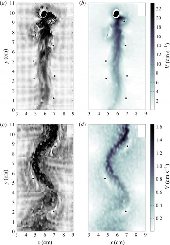
Figure 11. Illustration of the wake behind a single bubble (
 $Ar=1535$
) at two different times
$Ar=1535$
) at two different times
 $t=0.67~\text{s}$
and
$t=0.67~\text{s}$
and
 $t=2.5~\text{s}$
obtained by PIV measurements: (a,c) velocity vectors; (b,d) magnitude of the velocity; The dots indicate the centres of the vortices. (The region in the top-right corner is not explored due to insufficient lighting).
$t=2.5~\text{s}$
obtained by PIV measurements: (a,c) velocity vectors; (b,d) magnitude of the velocity; The dots indicate the centres of the vortices. (The region in the top-right corner is not explored due to insufficient lighting).

Figure 12. (a) Locations
 $x_{max}(y,t)$
corresponding to the maximal velocity
$x_{max}(y,t)$
corresponding to the maximal velocity
 $V_{max}$
in the wake of the bubble at different times
$V_{max}$
in the wake of the bubble at different times
 $t$
. The thick dashed line indicates the path followed by the bubble (around its mean horizontal position
$t$
. The thick dashed line indicates the path followed by the bubble (around its mean horizontal position
 $\overline{x_{b}}$
). The green vectors illustrate the orientation of the maximal velocity at
$\overline{x_{b}}$
). The green vectors illustrate the orientation of the maximal velocity at
 $t=1.3~\text{s}$
. (b) Evolution of
$t=1.3~\text{s}$
. (b) Evolution of
 $V_{max}$
as a function of the time
$V_{max}$
as a function of the time
 ${\it\delta}t$
relative to the passage of the bubble for several times
${\it\delta}t$
relative to the passage of the bubble for several times
 $t$
(brown curves) and for all times
$t$
(brown curves) and for all times
 $t$
(light grey curves). The black dashed line shows the average over all the measurements for a given
$t$
(light grey curves). The black dashed line shows the average over all the measurements for a given
 ${\it\delta}t$
. The evolution of the velocity at a given location is also drawn for comparison (blue dots). (Here,
${\it\delta}t$
. The evolution of the velocity at a given location is also drawn for comparison (blue dots). (Here,
 $Ar=1535$
.)
$Ar=1535$
.)

Figure 13. For various Archimedes numbers of regime B: (a) evolution of
 $V_{max}/\sqrt{gd}$
with the relative time
$V_{max}/\sqrt{gd}$
with the relative time
 ${\it\delta}t$
normalized with the viscous time scale
${\it\delta}t$
normalized with the viscous time scale
 ${\it\tau}_{{\it\nu}}$
; (b) normalization of the maximal value of
${\it\tau}_{{\it\nu}}$
; (b) normalization of the maximal value of
 $V_{max}$
with the gravitational velocity scale
$V_{max}$
with the gravitational velocity scale
 $\sqrt{gd}$
.
$\sqrt{gd}$
.
4.1. Ascending flow generated by the bubble
Figure 11 shows two snapshots of the PIV measurements of the flow induced by the motion of a bubble with
 $Ar=1535$
at the times
$Ar=1535$
at the times
 $t=0.67~\text{s}$
and
$t=0.67~\text{s}$
and
 $t=2.5~\text{s}$
. This bubble corresponds to a diameter
$t=2.5~\text{s}$
. This bubble corresponds to a diameter
 $d=6~\text{mm}$
, a mean vertical velocity
$d=6~\text{mm}$
, a mean vertical velocity
 $V_{b}=15.5~\text{cm}~\text{s}^{-1}$
and a frequency of oscillation
$V_{b}=15.5~\text{cm}~\text{s}^{-1}$
and a frequency of oscillation
 $f={\it\omega}/2{\rm\pi}=4.2~\text{Hz}$
, corresponding to the time period
$f={\it\omega}/2{\rm\pi}=4.2~\text{Hz}$
, corresponding to the time period
 $T_{x}=0.24~\text{s}$
. It does not belong to regime
$T_{x}=0.24~\text{s}$
. It does not belong to regime
 $B$
; however, it shares some common features with bubbles in this regime, and has been chosen to illustrate the larger extent in flow parameters of some results. At time
$B$
; however, it shares some common features with bubbles in this regime, and has been chosen to illustrate the larger extent in flow parameters of some results. At time
 $t=0.67~\text{s}$
(figure 11
a,b), the bubble is just leaving the PIV window. The presence of an ascending flow of decreasing amplitude behind the bubble is conspicuous. The presence of vortices is also clearly visible. These are materialized with a dot in their centre. Furthermore, we can observe an evolution in the shape of the ascending flow at larger times, associated with a change in the number of vortices present in the flow (figure 11
c,d for
$t=0.67~\text{s}$
(figure 11
a,b), the bubble is just leaving the PIV window. The presence of an ascending flow of decreasing amplitude behind the bubble is conspicuous. The presence of vortices is also clearly visible. These are materialized with a dot in their centre. Furthermore, we can observe an evolution in the shape of the ascending flow at larger times, associated with a change in the number of vortices present in the flow (figure 11
c,d for
 $t=2.5~\text{s}$
). To characterize the strength of the flow and its deformation in time, we determine at each vertical position
$t=2.5~\text{s}$
). To characterize the strength of the flow and its deformation in time, we determine at each vertical position
 $y$
the orientation,
$y$
the orientation,
 ${\it\theta}_{max}$
, the magnitude,
${\it\theta}_{max}$
, the magnitude,
 $V_{max}$
, and the location in the horizontal direction,
$V_{max}$
, and the location in the horizontal direction,
 $x_{max}$
, of the maximal velocity in the flow.
$x_{max}$
, of the maximal velocity in the flow.
Figure 12(a) shows how the line
 $x_{max}(y,t)$
corresponding to the maximal velocity in the wake of the bubble is deformed in time. The dashed line indicates the path followed by the bubble. We observe an upward displacement of the line that smoothes out in time. For the longer times, we see that the line converges towards a sinusoidal shape of larger amplitude than the bubble sinusoidal motion (approximately three times larger) and twice its period. We will come back to this aspect of the flow evolution when discussing the characteristics of the vortices in the next subsection. Besides bringing to the fore the deformation of the wake, the velocity
$x_{max}(y,t)$
corresponding to the maximal velocity in the wake of the bubble is deformed in time. The dashed line indicates the path followed by the bubble. We observe an upward displacement of the line that smoothes out in time. For the longer times, we see that the line converges towards a sinusoidal shape of larger amplitude than the bubble sinusoidal motion (approximately three times larger) and twice its period. We will come back to this aspect of the flow evolution when discussing the characteristics of the vortices in the next subsection. Besides bringing to the fore the deformation of the wake, the velocity
 $V_{max}$
provides a foremost characterization of the intensity of the flow generated by the bubble and how this is damped in space and time. For all
$V_{max}$
provides a foremost characterization of the intensity of the flow generated by the bubble and how this is damped in space and time. For all
 $Ar$
in regime B, velocities
$Ar$
in regime B, velocities
 $V_{max}$
larger than
$V_{max}$
larger than
 $V_{b}$
are observed in the wake until a distance from the bubble of approximately
$V_{b}$
are observed in the wake until a distance from the bubble of approximately
 $4d$
.
$4d$
.
The evolution in time of
 $V_{max}$
is obtained as follows. At a given time
$V_{max}$
is obtained as follows. At a given time
 $t$
corresponding to a PIV measurement, the velocity field provides a distribution
$t$
corresponding to a PIV measurement, the velocity field provides a distribution
 $V_{max}(y)$
. Now, for each
$V_{max}(y)$
. Now, for each
 $y$
, a relative time
$y$
, a relative time
 ${\it\delta}t$
elapsed since the passage of the bubble at the position
${\it\delta}t$
elapsed since the passage of the bubble at the position
 $y$
at the time
$y$
at the time
 $t_{0b}(y)$
can be defined as
$t_{0b}(y)$
can be defined as
 ${\it\delta}t=t-t_{0b}(y)$
. Therefore, each velocity field provides a short temporal segment of the evolution of
${\it\delta}t=t-t_{0b}(y)$
. Therefore, each velocity field provides a short temporal segment of the evolution of
 $V_{max}$
with
$V_{max}$
with
 ${\it\delta}t$
, as shown in figure 12(b) for some particular times
${\it\delta}t$
, as shown in figure 12(b) for some particular times
 $t$
ranging from
$t$
ranging from
 $0.6$
to 2.8 s. The mean evolution is then obtained by averaging the data corresponding to the same
$0.6$
to 2.8 s. The mean evolution is then obtained by averaging the data corresponding to the same
 ${\it\delta}t$
obtained for different values of
${\it\delta}t$
obtained for different values of
 $t$
and
$t$
and
 $y$
. This is shown with a dashed line in figure 12(b). The attenuation of the maximal velocity in the bubble wake is observed to evolve exponentially in time. A similar behaviour is observed for the velocity recorded in a fixed point (blue curve). Furthermore, two stages are visible. At shorter times,
$y$
. This is shown with a dashed line in figure 12(b). The attenuation of the maximal velocity in the bubble wake is observed to evolve exponentially in time. A similar behaviour is observed for the velocity recorded in a fixed point (blue curve). Furthermore, two stages are visible. At shorter times,
 ${\it\delta}t<1~\text{s}$
, the decrease of
${\it\delta}t<1~\text{s}$
, the decrease of
 $V_{max}$
corresponds to approximately 80 % of its peak value, while at longer times the attenuation of the velocity is still exponential but slower.
$V_{max}$
corresponds to approximately 80 % of its peak value, while at longer times the attenuation of the velocity is still exponential but slower.
Figure 13(a) shows that the same behaviour is observed for all the Archimedes numbers in regime B. In this figure,
 $V_{max}$
is normalized with the gravitational velocity scale
$V_{max}$
is normalized with the gravitational velocity scale
 $\sqrt{gd}$
. Figure 13(b) shows that this scale matches remarkably well the maximal value of
$\sqrt{gd}$
. Figure 13(b) shows that this scale matches remarkably well the maximal value of
 $V_{max}$
for all
$V_{max}$
for all
 $Ar\geqslant 1800$
. In figure 13(a), the time is normalized with the viscous time scale
$Ar\geqslant 1800$
. In figure 13(a), the time is normalized with the viscous time scale
 ${\it\tau}_{{\it\nu}}=h^{2}/(4{\it\nu})\simeq 2.3~\text{s}$
. The initial sharp decrease of
${\it\tau}_{{\it\nu}}=h^{2}/(4{\it\nu})\simeq 2.3~\text{s}$
. The initial sharp decrease of
 $V_{max}$
occurs in a time period shorter than
$V_{max}$
occurs in a time period shorter than
 ${\it\tau}_{{\it\nu}}$
, which corresponds to approximately two periods of oscillation
${\it\tau}_{{\it\nu}}$
, which corresponds to approximately two periods of oscillation
 $T_{x}$
. The decrease of the intensity of the ascending flow is then given by
$T_{x}$
. The decrease of the intensity of the ascending flow is then given by
 $V_{max}/\sqrt{gd}\simeq \exp (-{\it\gamma}{\it\delta}t/T_{x})$
with
$V_{max}/\sqrt{gd}\simeq \exp (-{\it\gamma}{\it\delta}t/T_{x})$
with
 ${\it\gamma}=0.6$
for a large range of bubble diameters
${\it\gamma}=0.6$
for a large range of bubble diameters
 $0.6\leqslant d\leqslant 1.3~\text{cm}$
corresponding to oscillating bubbles. Beyond
$0.6\leqslant d\leqslant 1.3~\text{cm}$
corresponding to oscillating bubbles. Beyond
 ${\it\delta}t\approx {\it\tau}_{{\it\nu}}/2$
, we observe that
${\it\delta}t\approx {\it\tau}_{{\it\nu}}/2$
, we observe that
 $V_{max}$
decreases as
$V_{max}$
decreases as
 $\exp (-2.5{\it\delta}t/{\it\tau}_{{\it\nu}})$
for all
$\exp (-2.5{\it\delta}t/{\it\tau}_{{\it\nu}})$
for all
 $Ar$
. This exponential decrease of the flow intensity occurring on the viscous time scale was also observed by Roig et al. (Reference Roig, Roudet, Risso and Billet2012) in their experiments for a 1 mm gap width, where
$Ar$
. This exponential decrease of the flow intensity occurring on the viscous time scale was also observed by Roig et al. (Reference Roig, Roudet, Risso and Billet2012) in their experiments for a 1 mm gap width, where
 ${\it\tau}_{{\it\nu}}$
is approximately ten times shorter and comparable to the time period
${\it\tau}_{{\it\nu}}$
is approximately ten times shorter and comparable to the time period
 $T_{x}$
. During this stage, viscous friction at the channel walls is predominant and the behaviour can be compared with the prediction for the attenuation of a Poiseuille flow in a thin channel due to viscous friction.
$T_{x}$
. During this stage, viscous friction at the channel walls is predominant and the behaviour can be compared with the prediction for the attenuation of a Poiseuille flow in a thin channel due to viscous friction.
Let us assume that the velocity induced by the bubble corresponds to the following Poiseuille velocity profile in the gap of the cell:
 $$\begin{eqnarray}\displaystyle \boldsymbol{u}=3/2\langle \boldsymbol{u}\rangle (1-4z^{2}/h^{2}), & & \displaystyle\end{eqnarray}$$
where
 $\langle \boldsymbol{u}\rangle$
is the mean velocity and corresponds to the PIV measurement (§ 2). Following Gondret & Rabaud (Reference Gondret and Rabaud1997), the Navier–Stokes equations averaged over the gap of the cell are
$\langle \boldsymbol{u}\rangle$
is the mean velocity and corresponds to the PIV measurement (§ 2). Following Gondret & Rabaud (Reference Gondret and Rabaud1997), the Navier–Stokes equations averaged over the gap of the cell are
 $$\begin{eqnarray}{\it\rho}\frac{\partial \langle \boldsymbol{u}\rangle }{\partial t}+\frac{6}{5}{\it\rho}(\langle \boldsymbol{u}\rangle \boldsymbol{\cdot }\boldsymbol{{\rm\nabla}})\langle \boldsymbol{u}\rangle =-\boldsymbol{{\rm\nabla}}p+{\it\mu}{\rm\Delta}_{xy}\langle \boldsymbol{u}\rangle -\frac{12{\it\mu}}{h^{2}}\langle \boldsymbol{u}\rangle ,\end{eqnarray}$$
where
 ${\rm\Delta}_{xy}$
is the Laplacian operator in the plane of the cell
${\rm\Delta}_{xy}$
is the Laplacian operator in the plane of the cell
 $(x,y)$
. Neglecting the friction in the plane of the cell and considering
$(x,y)$
. Neglecting the friction in the plane of the cell and considering
 $6/5\approx 1$
, we obtain
$6/5\approx 1$
, we obtain
 $$\begin{eqnarray}\displaystyle \frac{\text{d}\langle \boldsymbol{u}\rangle }{\text{d}t}=-\boldsymbol{{\rm\nabla}}p-\frac{12{\it\nu}}{h^{2}}\langle \boldsymbol{u}\rangle . & & \displaystyle\end{eqnarray}$$
Assuming that the pressure is constant leads to an exponential decrease of the averaged velocity as (Roig et al. Reference Roig, Roudet, Risso and Billet2012)
 $$\begin{eqnarray}\langle \boldsymbol{u}\rangle \sim \exp \left(-\frac{12{\it\nu}}{h^{2}}t\right)\sim \exp (-3t/{\it\tau}_{{\it\nu}}),\end{eqnarray}$$
which is slightly faster than the decrease measured experimentally.
A more accurate prediction can be obtained by considering now that the motion of the bubble induces over a time period
 $T_{i}$
a short impulse of pressure on the surrounding liquid, so that the resulting velocity profile in the gap is the solution of the following equation:
$T_{i}$
a short impulse of pressure on the surrounding liquid, so that the resulting velocity profile in the gap is the solution of the following equation:
 $$\begin{eqnarray}\frac{\partial \boldsymbol{u}(z,t)}{\partial t}=\boldsymbol{K}(H(t)-H(t-T_{i}))+{\it\nu}\frac{\partial ^{2}\boldsymbol{u}(z,t)}{\partial z^{2}},\end{eqnarray}$$
where
 $H$
is the Heaviside function and
$H$
is the Heaviside function and
 $\boldsymbol{K}$
is a constant pressure gradient. Using the Laplace transform and the theory of residues (Whittaker & Watson Reference Whittaker and Watson1927), we obtain the analytical solution
$\boldsymbol{K}$
is a constant pressure gradient. Using the Laplace transform and the theory of residues (Whittaker & Watson Reference Whittaker and Watson1927), we obtain the analytical solution
 $$\begin{eqnarray}\displaystyle u(z,t)=\frac{K}{2{\it\nu}}\left[\left(z^{2}-\frac{h^{2}}{4}\right)(1-H(t-T_{i}))+(1+\exp (-T_{i}))F(z,t)\right], & & \displaystyle\end{eqnarray}$$
with
 $$\begin{eqnarray}\displaystyle F(z,t)=\mathop{\sum }_{n=0}^{\infty }(-1)^{n}\frac{8h^{2}}{{\rm\pi}^{3}(2n+1)^{3}}\exp \left(-\frac{{\rm\pi}^{2}}{h^{2}}{\it\nu}(2n+1)^{2}t\right)\cos \left(\frac{{\rm\pi}}{h}(2n+1)z\right). & & \displaystyle\end{eqnarray}$$
The velocity averaged over the gap,
 $\langle u\rangle$
, has been calculated numerically. We choose
$\langle u\rangle$
, has been calculated numerically. We choose
 $T_{i}$
as the inertial time scale associated with the bubble,
$T_{i}$
as the inertial time scale associated with the bubble,
 $T_{i}=d/V_{b}$
. The norm of
$T_{i}=d/V_{b}$
. The norm of
 $\boldsymbol{K}$
is prescribed in order to match the averaged velocity at time
$\boldsymbol{K}$
is prescribed in order to match the averaged velocity at time
 $T_{i}$
with the velocity of the bubble,
$T_{i}$
with the velocity of the bubble,
 $\langle u\rangle (t=T_{i})=V_{b}$
. The evolution in time of the velocity profile is shown in figure 14. At short times (
$\langle u\rangle (t=T_{i})=V_{b}$
. The evolution in time of the velocity profile is shown in figure 14. At short times (
 $t\ll {\it\tau}_{{\it\nu}}$
), the velocity profile is close to plug flow, while at longer times (
$t\ll {\it\tau}_{{\it\nu}}$
), the velocity profile is close to plug flow, while at longer times (
 $t>{\it\tau}_{{\it\nu}}$
), viscous dissipation at the walls drives the velocity profile towards a parabolic shape. However, small differences remain, as can be seen from the Poiseuille velocity profiles drawn for comparison in figure 14 (dotted curves). The decrease of the velocity averaged over the gap given by (4.6) is then exponential and dominated by mode
$t>{\it\tau}_{{\it\nu}}$
), viscous dissipation at the walls drives the velocity profile towards a parabolic shape. However, small differences remain, as can be seen from the Poiseuille velocity profiles drawn for comparison in figure 14 (dotted curves). The decrease of the velocity averaged over the gap given by (4.6) is then exponential and dominated by mode
 $n=0$
. This mode corresponds to the following expression of the velocity:
$n=0$
. This mode corresponds to the following expression of the velocity:
 $$\begin{eqnarray}\langle u\rangle (t\rightarrow \infty )\sim \exp \left(-\frac{{\rm\pi}^{2}}{4}t/{\it\tau}_{{\it\nu}}\right)\sim \exp (-2.5t/{\it\tau}_{{\it\nu}}).\end{eqnarray}$$
The rate of decrease is slightly slower than the value corresponding to a Poiseuille velocity profile (4.4). Figure 13(a) shows the very good agreement of this prediction with the long-time evolution of the experimental measurements for
 $V_{max}$
.
$V_{max}$
.

Figure 14. Temporal decay of the flow in a thin channel generated by a pressure gradient applied during a finite time
 $T_{i}$
(inertial time scale associated with a bubble with
$T_{i}$
(inertial time scale associated with a bubble with
 $Ar=1535$
). At given times, the flow is compared with the parabolic velocity profiles corresponding to the same maximal velocities (dotted curves).
$Ar=1535$
). At given times, the flow is compared with the parabolic velocity profiles corresponding to the same maximal velocities (dotted curves).
4.2. Birth, life and death of the vortices released by a bubble
In strong interaction with the central mainly ascending flow, a vortex street is generated by the bubble as it rises in the cell. A major focus of the present investigation is to characterize the properties of these vortices. Figure 15(a) presents for
 $Ar=1535$
the evolution in time of the vorticity of the vortices released by the bubble during its rise in the PIV window. A periodic and alternate release of vortices of opposite vorticity is observed. The tracking procedure shows for each vortex an increase of the vorticity until the value
$Ar=1535$
the evolution in time of the vorticity of the vortices released by the bubble during its rise in the PIV window. A periodic and alternate release of vortices of opposite vorticity is observed. The tracking procedure shows for each vortex an increase of the vorticity until the value
 ${\it\Omega}_{0}$
reached at time
${\it\Omega}_{0}$
reached at time
 $t_{0}$
and then an attenuation in time. Since vorticity is generated at the bubble surface and evacuated in the flow through vortex shedding, we further consider that a vortex is released when its maximal vorticity is reached (time
$t_{0}$
and then an attenuation in time. Since vorticity is generated at the bubble surface and evacuated in the flow through vortex shedding, we further consider that a vortex is released when its maximal vorticity is reached (time
 $t_{0}$
). The attenuation in time occurring after vortex shedding is shown in logarithmic scale in figure 15(b), using the relative time
$t_{0}$
). The attenuation in time occurring after vortex shedding is shown in logarithmic scale in figure 15(b), using the relative time
 $t-t_{0}$
. The curve corresponds to the average of the vorticity decrease measured for the seven vortices shed in the PIV window by a bubble with
$t-t_{0}$
. The curve corresponds to the average of the vorticity decrease measured for the seven vortices shed in the PIV window by a bubble with
 $Ar=1535$
. As observed for the maximal velocity
$Ar=1535$
. As observed for the maximal velocity
 $V_{max}$
, two stages are conspicuous. The first corresponds to a fast decrease of vorticity (in this case, approximately 90 % of the initial vorticity is lost in 0.5 s), while the final stage of vortex dynamics occurs for times comparable to the viscous time scale
$V_{max}$
, two stages are conspicuous. The first corresponds to a fast decrease of vorticity (in this case, approximately 90 % of the initial vorticity is lost in 0.5 s), while the final stage of vortex dynamics occurs for times comparable to the viscous time scale
 ${\it\tau}_{{\it\nu}}$
, and corresponds to a slower exponential decrease in time of the vorticity. At long times (
${\it\tau}_{{\it\nu}}$
, and corresponds to a slower exponential decrease in time of the vorticity. At long times (
 $t-t_{0}>1~\text{s}$
), only two vortices remain in this example and five vortices disappear due to vortex interactions at intermediate times
$t-t_{0}>1~\text{s}$
), only two vortices remain in this example and five vortices disappear due to vortex interactions at intermediate times
 $(0.25~\text{s}<t-t_{0}<1~\text{s})$
.
$(0.25~\text{s}<t-t_{0}<1~\text{s})$
.

Figure 15. (a) Evolution in time of the vorticity of the vortices periodically released by the bubble during its rise. (b) Averaged evolution for all the vortices as a function of time relative to vortex shedding
 $t-t_{0}$
; the grey dots represent the superposed vorticity evolutions for the seven released vortices; the black curve corresponds to the averaged evolution. (
$t-t_{0}$
; the grey dots represent the superposed vorticity evolutions for the seven released vortices; the black curve corresponds to the averaged evolution. (
 $Ar=1535$
).
$Ar=1535$
).

Figure 16. Normalizations considered for the vorticity of a vortex at the time of release. (The error bar is the standard deviation for all of the released vortices recorded at a given
 $Ar$
.)
$Ar$
.)

Figure 17. For various Archimedes numbers of regime B: evolution of the vorticity
 ${\it\Omega}d/(V_{b}{\it\chi}^{3/2})$
with the relative time
${\it\Omega}d/(V_{b}{\it\chi}^{3/2})$
with the relative time
 $t-t_{0}$
normalized with (a) the period of oscillation
$t-t_{0}$
normalized with (a) the period of oscillation
 $T_{x}$
, (b) the viscous time scale
$T_{x}$
, (b) the viscous time scale
 ${\it\tau}_{{\it\nu}}$
. The model corresponds to
${\it\tau}_{{\it\nu}}$
. The model corresponds to
 ${\sim}\!\exp (-2.5t/{\it\tau}_{{\it\nu}})$
.
${\sim}\!\exp (-2.5t/{\it\tau}_{{\it\nu}})$
.
We now generalize this analysis for all of the bubbles in the B regime. The maximal vorticity
 ${\it\Omega}_{0}$
of the vortices at the time of release is provided by the vorticity produced at the bubble surface, an estimation of which is given by
${\it\Omega}_{0}$
of the vortices at the time of release is provided by the vorticity produced at the bubble surface, an estimation of which is given by
 $V_{b}/d$
. Figure 16(a) shows that this scaling underestimates the value of
$V_{b}/d$
. Figure 16(a) shows that this scaling underestimates the value of
 ${\it\Omega}_{0}$
, increasingly so as
${\it\Omega}_{0}$
, increasingly so as
 $Ar$
increases. A more accurate estimation is obtained by taking into account the anisotropy of the bubble. The vorticity generated at the bubble surface is estimated using a shorter length scale, which is the radius of curvature at the equator, where the curvature is the highest, yielding the scaling
$Ar$
increases. A more accurate estimation is obtained by taking into account the anisotropy of the bubble. The vorticity generated at the bubble surface is estimated using a shorter length scale, which is the radius of curvature at the equator, where the curvature is the highest, yielding the scaling
 $V_{b}{\it\chi}^{3/2}/d$
(determined with the ellipse corresponding to the bubble contour). Figure 16(b) shows that this quantity provides a good estimation of
$V_{b}{\it\chi}^{3/2}/d$
(determined with the ellipse corresponding to the bubble contour). Figure 16(b) shows that this quantity provides a good estimation of
 ${\it\Omega}_{0}$
for the whole range of Archimedes numbers. Once the vortices are released, their vorticity starts to decrease. Figure 17(a) shows that the decrease is sharp (approximately 80 % of
${\it\Omega}_{0}$
for the whole range of Archimedes numbers. Once the vortices are released, their vorticity starts to decrease. Figure 17(a) shows that the decrease is sharp (approximately 80 % of
 ${\it\Omega}_{0}$
is lost) in one period of oscillation of the bubble,
${\it\Omega}_{0}$
is lost) in one period of oscillation of the bubble,
 $T_{x}$
, identically for all the Archimedes numbers. This result suggests that the build-up of subsequent vortices by the bubble to evacuate in the surrounding flow the vorticity generated at its surface contributes strongly to the decrease of the vorticity of a released vortex. Vortex interaction is even more visible in the next stage. In between
$T_{x}$
, identically for all the Archimedes numbers. This result suggests that the build-up of subsequent vortices by the bubble to evacuate in the surrounding flow the vorticity generated at its surface contributes strongly to the decrease of the vorticity of a released vortex. Vortex interaction is even more visible in the next stage. In between
 $2$
and
$2$
and
 $5$
$5$
 $T_{x}$
, the vortex street undergoes a rearrangement. Vortex pairing occurs on both sides of the vortex street, leading to a vortex street of double wavelength. It is interesting to point out that only very few studies have measured at short times the evolution of a vortex street generated by a fixed solid body in an incoming flow. The work by Cimbala, Nagib & Roshko (Reference Cimbala, Nagib and Roshko1988), which investigates the origin of the large structures observed in the far wake of a fixed solid body and the role of vortex pairing, shows evidence for an exponential decrease of the intensity of the vortices associated with vortex interaction and amalgamation. Then, when
$T_{x}$
, the vortex street undergoes a rearrangement. Vortex pairing occurs on both sides of the vortex street, leading to a vortex street of double wavelength. It is interesting to point out that only very few studies have measured at short times the evolution of a vortex street generated by a fixed solid body in an incoming flow. The work by Cimbala, Nagib & Roshko (Reference Cimbala, Nagib and Roshko1988), which investigates the origin of the large structures observed in the far wake of a fixed solid body and the role of vortex pairing, shows evidence for an exponential decrease of the intensity of the vortices associated with vortex interaction and amalgamation. Then, when
 $t$
becomes of the order of
$t$
becomes of the order of
 ${\it\tau}_{{\it\nu}}$
in our configuration, viscous friction becomes the predominant effect. Using the same approach as in the previous section, an equation for the vorticity averaged over the gap width,
${\it\tau}_{{\it\nu}}$
in our configuration, viscous friction becomes the predominant effect. Using the same approach as in the previous section, an equation for the vorticity averaged over the gap width,
 $\langle {\it\bf\Omega}\rangle$
, can be retrieved from (4.2),
$\langle {\it\bf\Omega}\rangle$
, can be retrieved from (4.2),
 $\text{d}\langle {\it\bf\Omega}\rangle /\text{d}t=-12{\it\nu}/h^{2}\langle {\it\bf\Omega}\rangle$
, so that the vorticity is expected to decrease exponentially as
$\text{d}\langle {\it\bf\Omega}\rangle /\text{d}t=-12{\it\nu}/h^{2}\langle {\it\bf\Omega}\rangle$
, so that the vorticity is expected to decrease exponentially as
 $\exp (-3t/{\it\tau}_{{\it\nu}})$
. This expression provides an estimation of the damping of the vortex street at long times. However, in the experiments, the time scale of the decrease is close to
$\exp (-3t/{\it\tau}_{{\it\nu}})$
. This expression provides an estimation of the damping of the vortex street at long times. However, in the experiments, the time scale of the decrease is close to
 ${\it\tau}_{{\it\nu}}/2.5$
, as shown in figure 17(b). This result is in agreement with the decrease rate found for the mean velocity in expression (4.8). The same mechanism of viscous friction at the wall drives the attenuation of a vortex generated in a shallow water pool, as highlighted in the analysis carried out by Satijn et al. (Reference Satijn, Cense, Verzicco, Clercx and van Heijst2001), yielding the same decrease rate.
${\it\tau}_{{\it\nu}}/2.5$
, as shown in figure 17(b). This result is in agreement with the decrease rate found for the mean velocity in expression (4.8). The same mechanism of viscous friction at the wall drives the attenuation of a vortex generated in a shallow water pool, as highlighted in the analysis carried out by Satijn et al. (Reference Satijn, Cense, Verzicco, Clercx and van Heijst2001), yielding the same decrease rate.

Figure 18. The distance
 $D_{b{\it\Omega}_{0}}$
between the centre of the vortices and the centre of the bubble, at the time of release
$D_{b{\it\Omega}_{0}}$
between the centre of the vortices and the centre of the bubble, at the time of release
 $t_{0}$
, normalized with the bubble diameter
$t_{0}$
, normalized with the bubble diameter
 $d$
. (The error bar is the standard deviation for all of the released vortices recorded at a given
$d$
. (The error bar is the standard deviation for all of the released vortices recorded at a given
 $Ar$
.)
$Ar$
.)

Figure 19. Definition of the dimensions,
 $D_{\Vert }$
and
$D_{\Vert }$
and
 $D_{\bot }$
, characterizing the size and aspect ratio of the vortices. (a) Velocity field with the vortex centre, the axes
$D_{\bot }$
, characterizing the size and aspect ratio of the vortices. (a) Velocity field with the vortex centre, the axes
 $x^{\prime }$
and
$x^{\prime }$
and
 $y^{\prime }$
and the positions of the extrema of the velocities along these axes used to define
$y^{\prime }$
and the positions of the extrema of the velocities along these axes used to define
 $D_{\Vert }$
and
$D_{\Vert }$
and
 $D_{\bot }$
. (b) Velocity profile along the
$D_{\bot }$
. (b) Velocity profile along the
 $x^{\prime }$
axis. (c) Velocity profile along the
$x^{\prime }$
axis. (c) Velocity profile along the
 $y^{\prime }$
axis.
$y^{\prime }$
axis.

Figure 20. Evolution in time of the dimensions,
 $D_{\Vert }$
and
$D_{\Vert }$
and
 $D_{\bot }$
, for various Archimedes numbers in regime B. (Measurements are sometimes not available due to limitations of the automatic signal processing.)
$D_{\bot }$
, for various Archimedes numbers in regime B. (Measurements are sometimes not available due to limitations of the automatic signal processing.)
Up to now we have concentrated the discussion on the intensity of the vortices and their evolution in time. However, equal emphasis has to be given to complementary salient features of the vortices, which are their size and motion. Figure 18 shows that the distance
 $D_{b{\it\Omega}_{0}}$
between the centre of the vortices and the centre of the bubble, at the time of release
$D_{b{\it\Omega}_{0}}$
between the centre of the vortices and the centre of the bubble, at the time of release
 $t_{0}$
, is close to the characteristic diameter of the bubble
$t_{0}$
, is close to the characteristic diameter of the bubble
 $d$
, whatever the value of
$d$
, whatever the value of
 $Ar$
in the B regime. Once released, we observe a deformation and an expansion of the vortices (see figure 11). To get an estimation of the vortex size, we looked for nearby maximal velocities. We introduce two dimensions,
$Ar$
in the B regime. Once released, we observe a deformation and an expansion of the vortices (see figure 11). To get an estimation of the vortex size, we looked for nearby maximal velocities. We introduce two dimensions,
 $D_{\Vert }$
and
$D_{\Vert }$
and
 $D_{\bot }$
, determined at each time
$D_{\bot }$
, determined at each time
 $t$
. As explained in figure 19,
$t$
. As explained in figure 19,
 $D_{\bot }$
is calculated along the line
$D_{\bot }$
is calculated along the line
 $x^{\prime }$
joining the centre of the vortex to the position
$x^{\prime }$
joining the centre of the vortex to the position
 $x_{max}(y)$
such that
$x_{max}(y)$
such that
 $\boldsymbol{V}_{max}$
is perpendicular to this line. The azimuthal velocity profile of the vortex is determined along this line and
$\boldsymbol{V}_{max}$
is perpendicular to this line. The azimuthal velocity profile of the vortex is determined along this line and
 $D_{\bot }$
is defined as the distance separating the positions of highest positive and negative velocities (figure 19
b). In the same way, the azimuthal velocity profile of the vortex along the direction
$D_{\bot }$
is defined as the distance separating the positions of highest positive and negative velocities (figure 19
b). In the same way, the azimuthal velocity profile of the vortex along the direction
 $y^{\prime }$
perpendicular to the line of
$y^{\prime }$
perpendicular to the line of
 $D_{\bot }$
is used to determine the dimension
$D_{\bot }$
is used to determine the dimension
 $D_{\Vert }$
(figure 19
c). Figure 20(a,b) shows the evolution in time of these two quantities for various Archimedes numbers. At short times, the expansion of the vortices is observed first for
$D_{\Vert }$
(figure 19
c). Figure 20(a,b) shows the evolution in time of these two quantities for various Archimedes numbers. At short times, the expansion of the vortices is observed first for
 $D_{\bot }$
and then for
$D_{\bot }$
and then for
 $D_{\Vert }$
. At longer times, when the structure is frozen by viscous effects, we see that
$D_{\Vert }$
. At longer times, when the structure is frozen by viscous effects, we see that
 $D_{\bot }$
corresponds to approximately
$D_{\bot }$
corresponds to approximately
 $2.5d$
, while
$2.5d$
, while
 $D_{\Vert }$
scales with the spatial wavelength
$D_{\Vert }$
scales with the spatial wavelength
 ${\it\lambda}_{w}$
associated with the periodic motion of the bubble. The aspect ratio of the vortices is therefore proportional to the Strouhal number of the bubble, and as well to the aspect ratio
${\it\lambda}_{w}$
associated with the periodic motion of the bubble. The aspect ratio of the vortices is therefore proportional to the Strouhal number of the bubble, and as well to the aspect ratio
 ${\it\chi}$
of the bubble, for all
${\it\chi}$
of the bubble, for all
 $Ar$
in the B regime.
$Ar$
in the B regime.
We now turn our attention to the displacement of the vortices associated with the deformation and expansion of the vortex street. Figure 21(a,b) shows the evolution of the positions
 $x_{{\it\Omega}}$
(horizontal) and
$x_{{\it\Omega}}$
(horizontal) and
 $y_{{\it\Omega}}$
(vertical) of the centre of the vortices corresponding to the vorticities of figure 15(a). During the first stage lasting approximately two time periods
$y_{{\it\Omega}}$
(vertical) of the centre of the vortices corresponding to the vorticities of figure 15(a). During the first stage lasting approximately two time periods
 $T_{x}$
, and corresponding to the stronger decrease of vorticity and the increase of
$T_{x}$
, and corresponding to the stronger decrease of vorticity and the increase of
 $D_{\bot }$
, we observe that the vortices are moving outwards from the bubble path and upwards. When viscous dissipation becomes predominant (at approximately 1 s), the structure of the vortex street is frozen and the vortices simply decay in place. Only three vortices remain at long times in the PIV window as a result of vortex pairing. It should be noted that the dashed line corresponds to a vortex that was shed outside the PIV window and later entered the window. A key element of the vortex motion is therefore the orientation and amplitude of its velocity at the time of release
$D_{\bot }$
, we observe that the vortices are moving outwards from the bubble path and upwards. When viscous dissipation becomes predominant (at approximately 1 s), the structure of the vortex street is frozen and the vortices simply decay in place. Only three vortices remain at long times in the PIV window as a result of vortex pairing. It should be noted that the dashed line corresponds to a vortex that was shed outside the PIV window and later entered the window. A key element of the vortex motion is therefore the orientation and amplitude of its velocity at the time of release
 $t_{0}$
. Figure 22(a) shows the values of the horizontal (black symbols) and vertical (green symbols) components of the release velocity, denoted
$t_{0}$
. Figure 22(a) shows the values of the horizontal (black symbols) and vertical (green symbols) components of the release velocity, denoted
 $V_{x{\it\Omega}_{0}}$
and
$V_{x{\it\Omega}_{0}}$
and
 $V_{y{\it\Omega}_{0}}$
respectively, as the Archimedes number is increased. The vertical component is significantly higher than the horizontal one for all
$V_{y{\it\Omega}_{0}}$
respectively, as the Archimedes number is increased. The vertical component is significantly higher than the horizontal one for all
 $Ar$
in regime B (
$Ar$
in regime B (
 $1800\leqslant Ar\leqslant 5000$
). Furthermore, the initial velocity of a vortex at the time of release is compared with the velocity of the bubble in figure 23 for various Archimedes numbers. The velocity of the vortex is indicated with a thick black arrow placed in the vortex centre, while the corresponding instantaneous velocity of the bubble is shown with a red arrow. We can observe that vortex shedding occurs for significant different instantaneous velocities of the bubbles as
$1800\leqslant Ar\leqslant 5000$
). Furthermore, the initial velocity of a vortex at the time of release is compared with the velocity of the bubble in figure 23 for various Archimedes numbers. The velocity of the vortex is indicated with a thick black arrow placed in the vortex centre, while the corresponding instantaneous velocity of the bubble is shown with a red arrow. We can observe that vortex shedding occurs for significant different instantaneous velocities of the bubbles as
 $Ar$
increases in the B regime. Interestingly, we can also observe in this figure that there is a correspondence between the initial velocity of the vortex and the maximal velocity in the wake at the position
$Ar$
increases in the B regime. Interestingly, we can also observe in this figure that there is a correspondence between the initial velocity of the vortex and the maximal velocity in the wake at the position
 $y_{{\it\Omega}}$
of the vortex centre,
$y_{{\it\Omega}}$
of the vortex centre,
 $\boldsymbol{V}_{max,0}$
. This velocity is outlined with a blue arrow, while the line of vectors
$\boldsymbol{V}_{max,0}$
. This velocity is outlined with a blue arrow, while the line of vectors
 $\boldsymbol{V}_{max}$
corresponds to the thin black arrows. Comparison of the components of the velocity of a vortex at the time of release to the components of
$\boldsymbol{V}_{max}$
corresponds to the thin black arrows. Comparison of the components of the velocity of a vortex at the time of release to the components of
 $\boldsymbol{V}_{max,0}$
is presented in figure 22(b), showing that both velocities share approximately the same orientation. The structure of the flow in the wake of the bubble therefore drives the motion of the vortices at the time of release. Furthermore, the structure of the wake at
$\boldsymbol{V}_{max,0}$
is presented in figure 22(b), showing that both velocities share approximately the same orientation. The structure of the flow in the wake of the bubble therefore drives the motion of the vortices at the time of release. Furthermore, the structure of the wake at
 $t_{0}$
shown by figure 23 appears to be similar for all
$t_{0}$
shown by figure 23 appears to be similar for all
 $Ar$
in the B regime, although the instantaneous orientation and velocity of the bubbles are remarkably different for each
$Ar$
in the B regime, although the instantaneous orientation and velocity of the bubbles are remarkably different for each
 $Ar$
. This suggests that a more detailed analysis of the kinematics of the bubble at the time of release of a vortex is relevant.
$Ar$
. This suggests that a more detailed analysis of the kinematics of the bubble at the time of release of a vortex is relevant.

Figure 21. Evolution in time of the position of the centre of the vortices: (a) horizontal position
 $x_{{\it\Omega}}/d$
, (b) vertical position
$x_{{\it\Omega}}/d$
, (b) vertical position
 $y_{{\it\Omega}}/d$
. Same case as figure 15. The red curves correspond to the position of the centre of the bubble and the grey (respectively black) curves correspond to vortices on the right (respectively left) of the bubble. The continuous lines stand for vortices shed in the measurement field and the dashed lines for vortices shed out of the field of view.
$y_{{\it\Omega}}/d$
. Same case as figure 15. The red curves correspond to the position of the centre of the bubble and the grey (respectively black) curves correspond to vortices on the right (respectively left) of the bubble. The continuous lines stand for vortices shed in the measurement field and the dashed lines for vortices shed out of the field of view.

Figure 22. For various Archimedes numbers in regime B: horizontal (black symbols) and vertical (green symbols) components of the release velocity,
 $V_{x{\it\Omega}_{0}}$
and
$V_{x{\it\Omega}_{0}}$
and
 $V_{y{\it\Omega}_{0}}$
, of the vortices normalized (a) with
$V_{y{\it\Omega}_{0}}$
, of the vortices normalized (a) with
 $V_{b}$
, (b) with
$V_{b}$
, (b) with
 $V_{x_{max}}$
and
$V_{x_{max}}$
and
 $V_{y_{max}}$
, the horizontal and vertical components of the maximal velocity at the position
$V_{y_{max}}$
, the horizontal and vertical components of the maximal velocity at the position
 $y_{{\it\Omega}}$
of the vortex centre,
$y_{{\it\Omega}}$
of the vortex centre,
 $\boldsymbol{V}_{max,0}$
. (The error bar corresponds to the standard deviation for all the released vortices recorded at a given
$\boldsymbol{V}_{max,0}$
. (The error bar corresponds to the standard deviation for all the released vortices recorded at a given
 $Ar$
.)
$Ar$
.)
This brought to the fore a remarkable result shown in figure 24 for three values of
 $Ar$
in regime B and for
$Ar$
in regime B and for
 $Ar=1535$
. The magnitude of the transverse velocity of the bubble is maximal at the time of release, and thus equal to the amplitude
$Ar=1535$
. The magnitude of the transverse velocity of the bubble is maximal at the time of release, and thus equal to the amplitude
 $\tilde{V_{t}}$
investigated in § 3 (the magnitude of the velocity of the body is then also maximal at
$\tilde{V_{t}}$
investigated in § 3 (the magnitude of the velocity of the body is then also maximal at
 $t_{0}$
). This result uncovers the subtle relationship between the transverse velocity and the frequency of path oscillation, and thus of vortex shedding, already pointed out from the kinematics measurements (figure 9).
$t_{0}$
). This result uncovers the subtle relationship between the transverse velocity and the frequency of path oscillation, and thus of vortex shedding, already pointed out from the kinematics measurements (figure 9).

Figure 23. The structure of the flow in the near wake of a bubble for various values of
 $Ar$
(a, 1535; b, 1892; c, 2815; d, 4378) at the time
$Ar$
(a, 1535; b, 1892; c, 2815; d, 4378) at the time
 $t_{0}$
of vortex shedding. Thin grey arrows, instantaneous velocity field; thick black arrow, instantaneous velocity of the vortex; red arrow, instantaneous velocity of the bubble; thin black arrows, line of vectors
$t_{0}$
of vortex shedding. Thin grey arrows, instantaneous velocity field; thick black arrow, instantaneous velocity of the vortex; red arrow, instantaneous velocity of the bubble; thin black arrows, line of vectors
 $\boldsymbol{V}_{max}$
; blue arrow,
$\boldsymbol{V}_{max}$
; blue arrow,
 $\boldsymbol{V}_{max,0}$
, maximal velocity in the wake at the position
$\boldsymbol{V}_{max,0}$
, maximal velocity in the wake at the position
 $y_{{\it\Omega}}$
of the vortex centre.
$y_{{\it\Omega}}$
of the vortex centre.

Figure 24. Evolution in time of the transverse velocity
 $V_{t}$
. The circles indicate the times
$V_{t}$
. The circles indicate the times
 $t_{0}$
corresponding to vortex shedding extracted from the vortex tracking procedure;
$t_{0}$
corresponding to vortex shedding extracted from the vortex tracking procedure;
 $Ar=$
(a) 1535, (b) 1892, (c) 2815, (d) 4378.
$Ar=$
(a) 1535, (b) 1892, (c) 2815, (d) 4378.
5. Discussion
We revisited in the case of a cell having a larger gap the extensive and detailed investigation of the motion of bubbles freely rising in a thin-gap cell carried out by Roig et al. (Reference Roig, Roudet, Risso and Billet2012). The use of a cell having a larger gap for the same couple of fluids allowed us to separate the different time scales governing the motion of the bubble, so that
 $T_{i}\ll T_{x}\ll {\it\tau}_{{\it\nu}}$
, where
$T_{i}\ll T_{x}\ll {\it\tau}_{{\it\nu}}$
, where
 $T_{i}=d/V_{b}$
is the inertial time scale,
$T_{i}=d/V_{b}$
is the inertial time scale,
 $T_{x}$
is the period of path oscillation and of vortex shedding, and
$T_{x}$
is the period of path oscillation and of vortex shedding, and
 ${\it\tau}_{{\it\nu}}=h^{2}/(4{\it\nu})$
is the viscous time scale associated with the confinement width
${\it\tau}_{{\it\nu}}=h^{2}/(4{\it\nu})$
is the viscous time scale associated with the confinement width
 $h$
. Two steps towards the unification of the results for the two cells are achieved. For a given equivalent diameter
$h$
. Two steps towards the unification of the results for the two cells are achieved. For a given equivalent diameter
 $d$
of the bubble in the plane of the cell, the first is that the mean vertical velocity of the bubble is given by
$d$
of the bubble in the plane of the cell, the first is that the mean vertical velocity of the bubble is given by
 $V_{b}\simeq \sqrt{gr_{eq}}$
, where
$V_{b}\simeq \sqrt{gr_{eq}}$
, where
 $r_{eq}^{3}=(3/16)d^{2}h$
is the three-dimensional equivalent radius of the bubble; the second is that the mean vertical velocity of the bubble,
$r_{eq}^{3}=(3/16)d^{2}h$
is the three-dimensional equivalent radius of the bubble; the second is that the mean vertical velocity of the bubble,
 $V_{b}$
, determines at leading order the mean deformation of the bubble,
$V_{b}$
, determines at leading order the mean deformation of the bubble,
 ${\it\chi}$
, independently of the gap of the cell,
${\it\chi}$
, independently of the gap of the cell,
 $h$
. Equivalent aspect ratios of the bubble are in fact observed for the same
$h$
. Equivalent aspect ratios of the bubble are in fact observed for the same
 $Re$
in the two cells for the same couple of fluids, although the diameters of the bubble and their volumes are different (figure 6). Furthermore, a straightforward relationship is found for the mean aspect ratio of the bubble as a function of the Weber number,
$Re$
in the two cells for the same couple of fluids, although the diameters of the bubble and their volumes are different (figure 6). Furthermore, a straightforward relationship is found for the mean aspect ratio of the bubble as a function of the Weber number,
 ${\it\chi}\simeq 1.12We^{1/2}$
.
${\it\chi}\simeq 1.12We^{1/2}$
.
We investigated the kinematics of the bubble when its size
 $d$
increases. Three regimes of coupling between the motion, the shape and the wake of the bubble were distinguished, and emphasis was placed on the case of confined oscillating bubbles for which the diameter is larger than the channel gap (
$d$
increases. Three regimes of coupling between the motion, the shape and the wake of the bubble were distinguished, and emphasis was placed on the case of confined oscillating bubbles for which the diameter is larger than the channel gap (
 $h/d\leqslant 0.39$
, belonging to regime B). In this regime, a renewed understanding of the selection of the path of the bubbles was gained by analysing the kinematics in the reference frame associated with the bubble. For
$h/d\leqslant 0.39$
, belonging to regime B). In this regime, a renewed understanding of the selection of the path of the bubbles was gained by analysing the kinematics in the reference frame associated with the bubble. For
 $1800\leqslant Ar\leqslant 5000$
, the following properties of the bubble kinematics were uncovered: the mean axial velocity of the bubble is given by
$1800\leqslant Ar\leqslant 5000$
, the following properties of the bubble kinematics were uncovered: the mean axial velocity of the bubble is given by
 $V_{a}\simeq 0.92V_{b}$
, the dimensionless amplitude of the angular velocity is constant,
$V_{a}\simeq 0.92V_{b}$
, the dimensionless amplitude of the angular velocity is constant,
 $\tilde{r}d/V_{b}=St\tilde{{\it\beta}_{n}}\simeq 0.75$
, while that of the transverse velocity of the bubble scales as
$\tilde{r}d/V_{b}=St\tilde{{\it\beta}_{n}}\simeq 0.75$
, while that of the transverse velocity of the bubble scales as
 $\tilde{V_{t}}/V_{b}\simeq 0.33{\it\chi}$
, and the frequency of oscillation is given by
$\tilde{V_{t}}/V_{b}\simeq 0.33{\it\chi}$
, and the frequency of oscillation is given by
 $St=2{\rm\pi}fd/V_{b}\simeq 0.55{\it\chi}$
. Furthermore, the Strouhal number based on the transverse velocity component of the bubble
$St=2{\rm\pi}fd/V_{b}\simeq 0.55{\it\chi}$
. Furthermore, the Strouhal number based on the transverse velocity component of the bubble
 $\tilde{V_{t}}$
is constant,
$\tilde{V_{t}}$
is constant,
 $St^{\ast }=fd/\tilde{V_{t}}\simeq 0.27$
, giving a first clue about the subtle relationship between the transverse motion of the bubble and the frequency of path oscillation. Once the confinement ratio and the diameter of the bubble are known, the kinematics can be straightforwardly retrieved from these relationships, in which the aspect ratio of the bubble plays a crucial role.
$St^{\ast }=fd/\tilde{V_{t}}\simeq 0.27$
, giving a first clue about the subtle relationship between the transverse motion of the bubble and the frequency of path oscillation. Once the confinement ratio and the diameter of the bubble are known, the kinematics can be straightforwardly retrieved from these relationships, in which the aspect ratio of the bubble plays a crucial role.
We then turned our attention to the wake of the bubble and its evolution in time in the regime of confined oscillating bubbles (
 $1800\leqslant Ar\leqslant 5000$
). Careful experiments of HF PIV and an advanced procedure of analysis, including vortex tracking, allowed us to bring to light two main aspects of the flow generated by the bubble motion: the intensity of the ascending flow and the characteristics of the released vortices (vorticity, size and motion), as well as their evolution in time. The rise of the bubble generates a wake with a central mainly upward flow, where velocities of magnitude
$1800\leqslant Ar\leqslant 5000$
). Careful experiments of HF PIV and an advanced procedure of analysis, including vortex tracking, allowed us to bring to light two main aspects of the flow generated by the bubble motion: the intensity of the ascending flow and the characteristics of the released vortices (vorticity, size and motion), as well as their evolution in time. The rise of the bubble generates a wake with a central mainly upward flow, where velocities of magnitude
 $\sqrt{gd}$
are reached. Furthermore, velocities of magnitude larger than
$\sqrt{gd}$
are reached. Furthermore, velocities of magnitude larger than
 $V_{b}$
are found as far as
$V_{b}$
are found as far as
 $4d$
behind the bubble. When vortex shedding occurs, although the instantaneous inclination and velocity of the bubble are very different for each
$4d$
behind the bubble. When vortex shedding occurs, although the instantaneous inclination and velocity of the bubble are very different for each
 $Ar$
, the structure of the near wake appears to be similar for all values of
$Ar$
, the structure of the near wake appears to be similar for all values of
 $Ar$
and drives the motion of the vortex at the moment of detachment.
$Ar$
and drives the motion of the vortex at the moment of detachment.
A closer look at the kinematics of the bubble moreover revealed that the transverse velocity of the bubble reaches a maximum when vortex shedding occurs. In the theoretical framework of the generalized Kirchhoff’s equations, the torque due to the production of vorticity at the surface of the bubble
 ${\rm\Gamma}_{{\it\omega}}$
is balanced by two added-mass terms: (i) the torque
${\rm\Gamma}_{{\it\omega}}$
is balanced by two added-mass terms: (i) the torque
 ${\rm\Gamma}_{at}=(C_{Ma}-C_{Mt})V_{a}V_{t}$
, which depends on the anisotropy of the body (through the added-mass coefficients along the axial and transverse directions,
${\rm\Gamma}_{at}=(C_{Ma}-C_{Mt})V_{a}V_{t}$
, which depends on the anisotropy of the body (through the added-mass coefficients along the axial and transverse directions,
 $C_{Ma}$
and
$C_{Ma}$
and
 $C_{Mt}$
) and on the axial and transverse velocities of the bubble, and (ii) the torque
$C_{Mt}$
) and on the axial and transverse velocities of the bubble, and (ii) the torque
 ${\rm\Gamma}_{r}=J_{a}(\text{d}r/\text{d}t)$
proportional to the angular acceleration of the body and the added moment of inertia
${\rm\Gamma}_{r}=J_{a}(\text{d}r/\text{d}t)$
proportional to the angular acceleration of the body and the added moment of inertia
 $J_{a}$
(Mougin & Magnaudet Reference Mougin and Magnaudet2002a
). In their investigation for three-dimensional bubbles of spheroidal shape, Mougin & Magnaudet (Reference Mougin and Magnaudet2006) observed that the vortical torque is mainly balanced by the added-mass torque
$J_{a}$
(Mougin & Magnaudet Reference Mougin and Magnaudet2002a
). In their investigation for three-dimensional bubbles of spheroidal shape, Mougin & Magnaudet (Reference Mougin and Magnaudet2006) observed that the vortical torque is mainly balanced by the added-mass torque
 ${\rm\Gamma}_{at}$
. Interestingly, this result is also found for axisymmetric solid bodies by Fernandes et al. (Reference Fernandes, Ern, Risso and Magnaudet2008) and two-dimensional solid plates by Andersen, Pesavento & Wang (Reference Andersen, Pesavento and Wang2005), in spite of the additional angular acceleration associated in these cases with the proper moment of inertia of the bodies. Considering in our configuration the bubble as a two-dimensional ellipse of dimensionless added-mass coefficients
${\rm\Gamma}_{at}$
. Interestingly, this result is also found for axisymmetric solid bodies by Fernandes et al. (Reference Fernandes, Ern, Risso and Magnaudet2008) and two-dimensional solid plates by Andersen, Pesavento & Wang (Reference Andersen, Pesavento and Wang2005), in spite of the additional angular acceleration associated in these cases with the proper moment of inertia of the bodies. Considering in our configuration the bubble as a two-dimensional ellipse of dimensionless added-mass coefficients
 $C_{Ma}={\it\chi}$
and
$C_{Ma}={\it\chi}$
and
 $C_{Mt}=1/{\it\chi}$
, an estimation of the amplitudes of the torques can be obtained and shows that
$C_{Mt}=1/{\it\chi}$
, an estimation of the amplitudes of the torques can be obtained and shows that
 ${\rm\Gamma}_{r}$
represents 4–12 % of the magnitude of
${\rm\Gamma}_{r}$
represents 4–12 % of the magnitude of
 ${\rm\Gamma}_{at}$
in regime B. The amplitude of the vortical torque can then be estimated from
${\rm\Gamma}_{at}$
in regime B. The amplitude of the vortical torque can then be estimated from
 ${\rm\Gamma}_{at}$
, yielding
${\rm\Gamma}_{at}$
, yielding
 ${\rm\Gamma}_{{\it\omega}}/({\it\rho}{\rm\pi}abV_{b}^{2})=0.3({\it\chi}^{2}-1)$
, and showing its strong dependence on the bubble mean deformation. As pointed out in the investigation by Mougin & Magnaudet (Reference Mougin and Magnaudet2006) for a three-dimensional bubble, this result indicates that the bubble compensates the vortical torque by the creation of a drift angle and therefore of a transverse velocity, since the axial velocity component of the bubble is constant. Along the axial direction, in fact, the force balance is close to a gravity versus drag equilibrium, resulting in an almost constant axial velocity along the bubble path, as is also the case here. Furthermore, this result indicates that the vortical torque exerted on the bubble is close to maximal at the time of vortex shedding in our configuration, since
${\rm\Gamma}_{{\it\omega}}/({\it\rho}{\rm\pi}abV_{b}^{2})=0.3({\it\chi}^{2}-1)$
, and showing its strong dependence on the bubble mean deformation. As pointed out in the investigation by Mougin & Magnaudet (Reference Mougin and Magnaudet2006) for a three-dimensional bubble, this result indicates that the bubble compensates the vortical torque by the creation of a drift angle and therefore of a transverse velocity, since the axial velocity component of the bubble is constant. Along the axial direction, in fact, the force balance is close to a gravity versus drag equilibrium, resulting in an almost constant axial velocity along the bubble path, as is also the case here. Furthermore, this result indicates that the vortical torque exerted on the bubble is close to maximal at the time of vortex shedding in our configuration, since
 $V_{t}$
and
$V_{t}$
and
 ${\rm\Gamma}_{at}$
are maximal. This provides a second independent clue about the subtle relationship between the frequency of oscillation and the transverse velocity, vortex shedding imposing both the frequency of oscillation and the amplitude of
${\rm\Gamma}_{at}$
are maximal. This provides a second independent clue about the subtle relationship between the frequency of oscillation and the transverse velocity, vortex shedding imposing both the frequency of oscillation and the amplitude of
 $V_{t}$
through the torque balance on the bubble. Vortex shedding occurs when the bubble is no longer able to evacuate in an attached vortex the vorticity produced at its surface. At that moment, the vorticity of the vortex may be considered to be equal to the vorticity produced at the bubble surface. This was estimated here by
$V_{t}$
through the torque balance on the bubble. Vortex shedding occurs when the bubble is no longer able to evacuate in an attached vortex the vorticity produced at its surface. At that moment, the vorticity of the vortex may be considered to be equal to the vorticity produced at the bubble surface. This was estimated here by
 $V_{b}{\it\chi}^{3/2}/d$
, which takes into account the mean deformation of the bubble, showing a good agreement with the vorticity measurements at detachment.
$V_{b}{\it\chi}^{3/2}/d$
, which takes into account the mean deformation of the bubble, showing a good agreement with the vorticity measurements at detachment.
The following stages then emerged concerning the evolution in time of the wake generated by the bubble. For short times following vortex shedding, lasting approximately one to two periods of oscillation
 $T_{x}$
, a rapid decay of the vorticity of the released vortex is observed and may be attributed to the formation of the neighbouring vortices on both sides of the vortex street. Meanwhile, the released vortices located initially at a distance of approximately one diameter from the bubble centre move outwards from the bubble path and expand. At intermediate times, the vortex street undergoes a subharmonic instability (vortex pairing) leading to a vortex street with half the number of vortices. In the final stage corresponding to times of the order of the viscous time
$T_{x}$
, a rapid decay of the vorticity of the released vortex is observed and may be attributed to the formation of the neighbouring vortices on both sides of the vortex street. Meanwhile, the released vortices located initially at a distance of approximately one diameter from the bubble centre move outwards from the bubble path and expand. At intermediate times, the vortex street undergoes a subharmonic instability (vortex pairing) leading to a vortex street with half the number of vortices. In the final stage corresponding to times of the order of the viscous time
 ${\it\tau}_{{\it\nu}}$
, the vortex street becomes frozen, and the characteristic dimensions of the vortices scale with
${\it\tau}_{{\it\nu}}$
, the vortex street becomes frozen, and the characteristic dimensions of the vortices scale with
 ${\it\lambda}_{w}$
and
${\it\lambda}_{w}$
and
 $d$
, corresponding to an aspect ratio of the vortices proportional to
$d$
, corresponding to an aspect ratio of the vortices proportional to
 $St$
as well as to the bubble aspect ratio
$St$
as well as to the bubble aspect ratio
 ${\it\chi}$
. The flow structure then decays exponentially in place, as can be predicted by considering the attenuation in time of the mean velocity of a non-fully-established Poiseuille flow in the gap of the cell through viscous dissipation at the walls.
${\it\chi}$
. The flow structure then decays exponentially in place, as can be predicted by considering the attenuation in time of the mean velocity of a non-fully-established Poiseuille flow in the gap of the cell through viscous dissipation at the walls.
Acknowledgements
The authors are grateful to S. Cazin, M. Marchal, G. Ehses and J.-P. Escafit for the technical support provided for the experiments.


