


1. Introduction
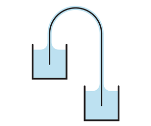
The siphon is widely used as a simple yet effective device to transfer liquid over the wall of a high container and into a lower container. A conventional siphon takes the form of a hook-shaped tube or pipe that bridges the containers, where fluid exits the higher source, climbs upwards over the arch, and then flows downwards to the receiver. If the flow is considered inviscid, incompressible and steady, Bernoulli's equation for conservation of energy predicts that the mean flow speed  $V$ depends on the height difference
  $H$ between the free surfaces of the containers:
  $V = \sqrt {2gH}$, where
  $g$ is the gravitational acceleration (Potter & Barnes Reference Potter and Barnes1971; White Reference White2015). How this flow is maintained and especially the roles played by atmospheric pressure (Ramette & Ramette Reference Ramette and Ramette2011; Richert & Binder Reference Richert and Binder2011) and intermolecular cohesion (Hughes Reference Hughes2010; Boatwright, Hughes & Barry Reference Boatwright, Hughes and Barry2015) in the upward flow from the source to the apex have been the subject of recent discussions. Nonetheless, it is clear that the tube of a standard siphon must be closed and that no cavitation occurs, otherwise the invasion of ambient air or vapour breaks the flow.
Siphon-like flows of some exotic fluids can be maintained even when open to the atmosphere. For example, a viscoelastic fluid continues to flow from a container after initiated by pouring over the side (James Reference James1966; Prokunin Reference Prokunin1983), since the internal stress serves as the ‘chain’ that supports and maintains the upwards flow. A second example is the so-called film flow of a superfluid in which liquid spontaneously climbs along the walls of a container and drains out (Rollin & Simon Reference Rollin and Simon1939; Fairbank & Lane Reference Fairbank and Lane1949).
Here we characterize open siphons of Newtonian fluids whose surface tension provide the ‘skin’ that sustains the flow. A demonstration of such a capillary siphon is the so-called walking water experiment (Sloane Reference Sloane1886; Guo & Cao Reference Guo and Cao2005; Ganci & Yegorenkov Reference Ganci and Yegorenkov2008) shown in figure 1(a). A piece of tissue paper bridges two cups, the left being initially filled with water (dyed blue) and the other empty. Water is spontaneously absorbed by the paper, rises by capillary action, and slowly collects into the right cup, stopping only when the heights equilibrate. The interstitial pores in the fibrous network of the tissue provide countless open conduits. In addition to characterizing the paper siphon, we introduce and study a minimal system consisting of capillary grooves in a wetting solid. This simple geometry permits a theoretical model that accurately predicts the siphon's flow characteristics by considering how gravity, surface tension and viscosity influence the shape of the water–air interface, the flow velocity and pressure. The groove and paper systems are shown to share properties fundamentally different from those of conventional siphons.

Figure 1. Paper siphons. (a) Walking water. Water in the left cup is spontaneously absorbed by folded paper tissue and transferred to the right cup. The water levels equilibrate after 10 h and the flow ceases. (b) A single-sheet paper siphon formed by filter paper draped over plastic disks. (c) Experimental schematic. The paper bridges source and receiver containers, and the steady-state volumetric flow rate  $Q$ is measured with a digital scale. The siphon head
  $h = 3.7$ cm is fixed while the height
  $H$ is varied. (d) The flux
  $Q$ increases then saturates with
  $H$. Inset: A log–log plot shows that
  $Q(H)$ does not follow the law
  $Q\sim \sqrt {H}$ of conventional siphons.
2. Experiments on paper and groove siphons
Here we introduce the paper and groove siphon systems and describe experimental characterizations of the dependence of flux on geometrical parameters.
2.1. Paper siphon
For the single-sheet paper siphon shown in figures 1(b) and 1(c), we measure the volumetric flow rate  $Q$ under conditions of fixed heights
  $h$ and
  $H$, the latter then varied. A long strip of filter paper (Whatman 1004-648 Grade 4 Qualitative Filter Paper, areal density 96 g
  $\text {m}^{-2}$, pore size 20 to 25
  $\mathrm {\mu }$m, width 3.8 cm) is cut to the desired length and hung over the edges of plastic supporting disks (diameter 2.54 cm). One end is immersed in the upper source container, where the water height is maintained by an overflow mechanism (not shown in figure 1c). The other end dips into the lower receiver container, which hangs from a high-precision digital scale (OHAUS model PX323, 0.001 g). The lower container's cross-section is sufficiently large to keep nearly constant water height during each measurement. An enclosure (not shown) over the whole set-up ensures high humidity and prevents evaporation.
Dynamic equilibrium is reached in several hours, as assessed by repeated measurements of the volumetric flow rate  $Q={\rm \Delta} m/\rho {\rm \Delta} t$, where
  ${\rm \Delta} m$ is the measured mass of water (density
  $\rho$) collected during the time interval
  ${\rm \Delta} t$ as measured with a stopwatch. For the results reported in figure 1(d), the head
  $h=3.7$ cm is fixed, and the measurement procedure is repeated several times for a given
  $H$, and this parameter is then systematically varied. Evidently, the flux
  $Q$ steeply increases with
  $H$ before saturating to a plateau. To facilitate comparison to the
  $Q\sim \sqrt H$ law for conventional siphons, we show a log–log plot of these data in the inset, where the paper siphon can be seen to deviate significantly from a line of slope 1/2. Linear behaviour of slope 1 for low
  $H$ transitions to the saturated response of slope 0 for high
  $H$, and these trends are shown in what follows to be general features of capillary siphoning.
2.2. Groove siphon
We next consider a related but simplified capillary siphon that takes the form of an arched groove in a wetting solid, this system being better controlled and whose geometry can be completely characterized. As shown schematically in figure 2(a), our experimental realization consists of two hook-shaped stainless-steel rods that are thoroughly cleaned and then firmly clamped together by procedures that are detailed below. The surface is hydrophilic, allowing water to wet the two narrow grooves between the rods, as shown in the cross-sectional view in figure 2(b). Each groove presents an open capillary channel whose geometry is uniform along its length.

Figure 2. Groove siphon. (a) Experimental realization of open channels or grooves formed by firmly pressing together two hook-shaped stainless-steel rods. (b) Cross-sectional view of grooves and wetted region. (c) Measurement apparatus. The flow rate  $Q$ through the groove siphon (dark hook shape) is measured by transferring, via a regular siphon, the collected water to a container hung below a digital scale. Mounting the components on vertical slides (not shown) allows the heights
  $h$ and
  $H$ to be varied independently.
We employ rods of radius  $R=0.24$ cm, and the inner radius of the arch is 1.03 cm. Flux measurements are carried out using the apparatus of figure 2(c), which is similar to the paper siphon system but with two modifications. First, mounting the components appropriately on vertical slides (not shown) allows
  $h$ and
  $H$ to be varied independently, thus enabling a more complete characterization. Second, because the collection chamber is deep to allow for a wide range of
  $H$, and to avoid exceeding the maximum allowable weight for the scale, we opt to transfer the collected water to a shallow container for the flux measurement. This is done via a regular tube siphon, and the flow rate
  $Q = \dot {m} (1+A_c/A_t)/\rho$ is calculated from the measured mass rate
  $\dot {m}$ and the cross-sectional areas
  $A_c$ and
  $A_t$ of the collector and transfer containers, respectively.
The groove siphon requires careful protocols for cleaning, assembly and priming. Before assembly, the rods and all other wetted components are gently scrubbed down with a soft sponge and soapy water and then rinsed thoroughly and repeatedly with filtered and deionized water. Since the wetting properties of stainless steel are known to be generally hydrophilic but sensitive to surface preparation (Prajitno, Maulana & Syarif Reference Prajitno, Maulana and Syarif2016; Terpiłowski et al. Reference Terpiłowski, Hołysz, Rymuszka and Banach2016), we directly measure the contact angle  $\theta = 27^{\circ } \pm 6^{\circ }$ in separate experiments using a horizontal microscope focused on the apex of the arch. For the siphon experiments, assembly is done immediately after cleaning. The rods are firmly clamped by tightening the screws of many two-piece stainless-steel shaft collars (not shown in figure 2) that are distributed along the entire length of the rods. Alignment and uniformity of the contact is checked by inspection of the groove with strong backlighting; no passed light indicates firm contact between the rods. After assembly, we prime the siphon by adding several water drops to the apex to thoroughly wet the grooves. The collars are in contact with the outer portions of the rods but not the inner portions that form the groove, thus avoiding any obstruction of the flow. The siphon then starts, and the system is again enclosed and found to reach steady state in about half an hour.
Figure 3(a) shows how  $Q$ depends on
  $H$ for two values of
  $h$, and the experimental data (red and blue dots) follow trends similar to those of the paper siphon. In particular, the linear increase in
  $Q(H)$ for low
  $H$ transitions to a plateau at higher
  $H$. Comparison of the two datasets shows that higher values of
  $h$ lead to weaker flows overall, that is, lower slopes of
  $Q(H)$ in the linear regime and lower values of the saturated flux. These trends are confirmed by systematic measurements of
  $Q(h)$ for fixed
  $H$, as shown by the green dots in figure 3(b) for
  $H=10.1$ cm. The flux
  $Q$ decreases monotonically and nonlinearly with the head
  $h$. Thus, unlike the conventional siphon, whose flux is independent of the head, the flow rate of the groove siphon is strongly modulated by changing
  $h$.
$h$.

Figure 3. Experimental (dots) and model (dashed curves) results for the groove siphon. (a) Flow rate  $Q$ versus siphon height
  $H$ for head values
  $h=2.2$ cm (blue) and
  $h=5.6$ cm (red). Shaded bands represent the variations in model predictions when contact angles are varied over the range
  $\theta \in [21^{\circ }, 33^{\circ }]$ measured in experiments. (b) Flow rate
  $Q$ versus siphon head
  $h$ for fixed
  $H=10.1$ cm.
3. Model of the groove siphon
To understand the characteristics of capillary siphoning, we formulate a theoretical model of the groove siphon, the predictions of which are compared to experiments.
3.1. Governing equations
Our model seeks to determine the flow rate through the groove siphon by considering how the shape of the wetted region varies along its length. The flow is assumed to be steady, laminar and well developed, as justified by the low Reynolds numbers  $Re = \rho l_c V/\mu \lesssim 1$ observed in experiments. Here
  $\rho = 1.0~\text {g}~\text {cm}^{-3}$ and
  $\mu = 0.89$ cP are the density and dynamic viscosity of water, respectively. The typical dimension of the cross-section is taken to be the capillary length scale
  $l_c = \sqrt {\gamma / \rho g} = 0.27$ cm, where
  $\gamma$ is the water–air surface tension coefficient. Assuming a characteristic flow speed
  $V=Q/l_c^2$, the experimentally measured range of
  $Q \sim 10^{-5} - 10^{-3}~\text {cm}^3~\text {s}^{-1}$ implies a range
  $Re \sim 10^{-2} - 10^0$. Further, since the length scale of the liquid in the groove cross-section is typically smaller than the total siphon length by an order of magnitude or more, the slender geometry motivates a simplifying approximation in which the pressure and velocity fields are homogenized by averaging within each cross-section. The section-averaged pressure
  $P$ and flow speed
  $V$, together with the shape of the wetted region, are descriptors of the system that vary with the position
  $s$ along the siphon axis. These quantities are related through three governing equations for mass conservation, the Young–Laplace law and the Stokes equation for low-Reynolds-number flow.
The model incorporates the detailed geometry and parameters relevant to our experimental system, though we expect the phenomenology and trends to hold more generally. Prescribed constants include the fluid density  $\rho$, dynamic viscosity
  $\mu$, contact angle
  $\theta$, rod radius
  $R$ as well as the hook-shaped path of the siphon axis, which determines the height function
  $z(s)$ (see figure 4a). For any arbitrary cross-section at location
  $s$, the liquid wets the solid through an angle of
  $\phi (s)$, as shown in figure 4(b). The free surface is assumed to be a circular arc with radius of curvature
  $r(s)$. Assuming uniform pressure over each cross-section, the Young–Laplace law for capillary pressure relates the internal pressure
  $P(s)$ to the shape of the wetted region:
 \begin{equation} P_0 - P(s) = \frac{\gamma}{r(s)}, \end{equation}
where  $P_0$ is atmospheric pressure. The slender geometry justifies the inclusion of only the interfacial curvature in the plane perpendicular to the siphon axis. The radius of curvature
  $r(s)$ relates to
  $\phi (s)$,
  $\theta$ and
  $R$,
$R$,
 \begin{equation} r = R \, \frac{1 - \cos \phi}{\cos (\phi+\theta)}, \end{equation}
which can be derived based on the assumed geometry of figure 4(b).

Figure 4. Model of the groove siphon. (a) Side view of the siphon. The arclength  $s$ marks position along the siphon axis, and
  $z$ is the vertical coordinate. (b) Cross-sectional view. Water wets the solid rods (radius
  $R$) with contact angle
  $\theta$. The wetted angle
  $\phi$ and radius of curvature
  $r$ of the air–water interface vary with
  $s$ and are to be determined by the model. (c) Zoomed-in view of the wetted region. The colour map shows an example numerical solution for the axial velocity field for steady, viscous flow with no-slip conditions on the solid and a stress-free interface. (d) Cross-sectional area
  $A$ (blue) of the wetted region and its mean pressure
  $P$ (red) for a representative solution of the model (
 $h=5$ cm and
  $H=7$ cm). The minima in these quantities (dotted line) occur somewhat downstream of the apex of the arch (dashed line).
Mass conservation demands that the product of wetted area  $A(s)$ and the mean speed
  $V(s)$ be uniformly constant along the siphon axis,
 \begin{equation} A(s)V(s) = Q, \end{equation}
where  $Q$ is the volumetric flow rate whose value we seek. The wetted area
  $A(s)$ at each cross-section also relates to
  $\phi (s)$,
  $\theta$ and
  $R$ via the specified geometry shown in figure 4(b):
 \begin{equation} A = R^2 (2\sin\phi - \sin\phi\cos\phi - \phi) - r^2\left[\frac{\rm \pi}{2}-\phi-\theta-\frac{1}{2}\sin(2\phi+2\theta)\right]. \end{equation}
This form reflects a particular approach to the geometric calculation, and many equivalent expressions exist, including those that use (3.2) to eliminate  $r$ in favour of
  $\phi$.
Considering the groove as a conduit whose cross-section dimensions vary slowly along the length (Tanner Reference Tanner1966; White Reference White2015), the one-dimensional Stokes equation for fully developed laminar flow takes the form
 \begin{equation} \frac{\mathrm{d}P(s)}{\mathrm{d}s} + \frac{\mu K V(s)}{2D_h^2(s)} + \rho g \frac{\mathrm{d}z(s)}{\mathrm{d}s} = 0, \end{equation}
which expresses the balance of axial pressure gradients with viscous and gravitational stresses. The second term can be understood as a hydraulic approximation that averages within each cross-section the viscous pressure gradient  $\mu \nabla ^2 v$ associated with the axial flow velocity field
  $v$. The non-circular cross-sectional geometry and its variations with arclength
  $s$ along the conduit are reflected in the effective hydraulic diameter
  $D_h(s) = 2A(s)/R\phi (s)$ and the dimensionless friction factor coefficient
  $K$ (Ayyaswamy, Catton & Edwards Reference Ayyaswamy, Catton and Edwards1974; Suh, Greif & Grigoropoulos Reference Suh, Greif and Grigoropoulos2001; White Reference White2015). The latter only depends on the shape of the wetted region but is found to be nearly identical across the family of shapes encountered here, as described in detail below.
Combining equations (3.1), (3.3) and (3.5) yields a boundary value problem for  $\phi (s)$ with
  $Q$ as an unknown coefficient to be determined:
 \begin{equation} f_1(\phi) \, \frac{\mathrm{d}\phi}{\mathrm{d}s} + f_2(\phi) \, Q + f_3(s) = 0, \end{equation}
with  $f_1(\phi ) = ({\gamma }/{r^2(\phi )})\,{\mathrm {d}r}/{\mathrm {d}\phi }$,
  $f_2(\phi ) = \frac {1}{8} \mu K R^2 \phi ^2 /A^3(\phi )$ and
  $f_3(s) = \rho g \,{\mathrm {d}z}/{\mathrm {d}s}$. Here
  $\phi (s)$ is regarded as the quantity of interest since
  $r$ and
  $A$ relate to
  $\phi$ via (3.2) and (3.4). The third term is prescribed by the siphon centreline and hence implicitly contains
  $h$ and
  $H$. The boundary conditions are given by the pressures being atmospheric at the two ends of the siphon, which implies via (3.1) that the cross-sectional interfaces are flat and thus
  $\phi (0) = \phi (L) = {\rm \pi}/2 - \theta$. Numerical solutions obtained via the MATLAB function bvp4c yield
  $Q$ and
  $\phi (s)$, and thus
  $r(s)$ and
  $A(s)$; these results will be discussed in detail in the sections that follow.
The friction factor  $K$ that appears in the viscous term of (3.5) and (3.6) is determined numerically by solving the open-channel flow problem for geometries of the type shown in figure 4(b). The two-dimensional (2-D) Poisson equation
  $\mu \nabla ^2 v = -G$ for axial velocity field
  $v$ and constant applied pressure gradient
  $G$ is solved using MATLAB's Partial Differential Equation Toolbox with no-slip boundary conditions on the solid boundaries and stress-free conditions on the interface. We systematically vary
  $\theta \in [21^{\circ }, 33^{\circ }]$ in order to account for the experimental variability in
  $\theta$ and also explore the full range of
  $\phi \in [0, {\rm \pi}/2-\theta ]$. Numerical solutions of the 2-D flow fields, an example of which is shown in figure 4(c), allow for the computation of the cross-sectional average speed
  $V$ across
  $\theta$ and
  $\phi$. The friction factor coefficient is then determined as
  $K = 2D_h^2 G/V$ and is found to vary at most between 26.3 and 28.9. Given this small range, we assume a constant
  $K = 27.6$, this value being an input to the boundary value problem described above.
3.2. Comparison of model and experiment
The model prediction of the flux  $Q$ for prescribed
  $H$ and
  $h$ is compared to experiments in figure 3. We investigate a range of values
  $\theta = 27^\circ \pm 6^\circ$ that spans the uncertainty in the experimental measurement of
  $\theta$. The results are shown in figures 3(a) and 3(b), where the dashed curves correspond to the mean value
  $\theta = 27^\circ$ and the shaded bands represent the results of varying
  $\theta$. The plots and insets show that the major trends are successfully reproduced by the model:
  $Q$ increases linearly with
  $H$ for small
  $H$, plateaus for large
  $H$, and strongly diminishes with increasing
  $h$. The model and experiment show fair quantitative agreement for high
  $H$, but the former tends to overestimate the linear rise of
  $Q$ for low
  $H$. Possible sources of this discrepancy are discussed below. Nonetheless, the flux magnitudes, scaling relations and qualitative trends seem to be robust. The strong agreement for large siphon heights and heads suggests that the model predictions may be accurate for values of
  $H$ and
  $h$ beyond those explored here.
The disagreement between model and experiment for low  $h$ and
  $H$ is likely to be due to three-dimensional (3-D) effects present in experiments near the ends of the siphon but which are not accounted for in the model. In particular, the meniscus geometry is complex where the rods meet the bath, as the liquid surface not only spans the grooves but also rises up from the bath to form contact lines that wrap around the rods. Consequently, the flow velocity field is expected to have significant non-axial components. Our model, on the other hand, assumes a slender geometry in which the cross-sectional shape and area change only slowly along the length of the siphon, and the flow is purely axial. These assumptions are quite reasonable for locations far from the ends, and indeed the model compares well when
  $h$ and
  $H$ are large, conditions for which end effects can reasonably be taken as negligible. An improved model would incorporate the 3-D nature of the meniscus, as has been considered for related geometries (Pozrikidis Reference Pozrikidis2010; Cooray, Cicuta & Vella Reference Cooray, Cicuta and Vella2012).
A benefit of the model is that it offers a detailed view of how the cross-sectional area of the wetted region and its pressure vary along the siphon axis, as shown in figure 4(d) for a representative case of  $H = 7$ cm and
  $h=5$ cm. The area
  $A(s)$ (blue) and pressure
  $P(s)$ (red) are maximal at the two ends and minimal at an intermediate arclength location
  $s$. The pressure curve is qualitatively similar to that of a conventional ideal siphon: the ends being in contact with the atmosphere requires that
  $P(0)=P(L)=P_0$, and
  $P(s)$ is otherwise lower than atmospheric pressure primarily because of the gravitational contribution. The area curve can be qualitatively interpreted through the coupling between the shape of the free surface and the pressure. The strongly negative gravitationally induced pressure along the upper portions of the siphon must be resisted by high curvature of the free interface, which is achieved by the surface retreating deeply into the groove and thus shrinking the wetted area. The changes in area are dramatic, steeply dropping upon exiting the source container, thinning by two orders of magnitude, and then rapidly rising in the approach to the collector. For typical parameters explored here, the wetted region shrinks to
  $A_{{min}} \sim 10^4~\mathrm {\mu }\text {m}^2$, equivalent to a length scale of about 100
  $\mathrm {\mu }\text {m}$ or roughly the width of a human hair.
In contrast to the conventional siphon, for which pressure is lowest at the apex, the minimal pressure and minimal area of the groove siphon occur somewhat displaced along the longer arm, as shown in figure 4(d). This fact can be interpreted by analysing the balance of pressures represented by (3.5). At the apex, the gravitational contribution is zero, and thus a negative pressure gradient is needed to drive the flow against viscous resistance. The negative gradient at the apex implies that the minimal value of pressure must occur downstream along the longer arm. The Young–Laplace law of (3.1) ensures that the cross-sectional area reaches a minimum at this same location.
3.3. Characterization via dimensionless quantities
The general characteristics of capillary siphoning can be revealed by recasting the model in dimensionless form and exploring a wide range of the relevant parameters. Non-dimensionalization is carried out by choosing length, velocity and pressure scales based on surface tension and viscous effects (De Gennes, Brochard-Wyart & Quéré Reference De Gennes, Brochard-Wyart and Quéré2013): capillary length  $l_c = \sqrt {\gamma /\rho g}$, velocity
  $V_c=\gamma /\mu$, flux
  $Q_c = V_c l_c^2$ and pressure
  $P_c=\gamma /l_c$. The solutions of the model can then be recast in terms of dimensionless volumetric flow rate
  $\tilde {Q} = Q / Q_c$ generated for given values of
  $\tilde {H} = H / l_c$ and
  $\tilde {h} = h / l_c$. For simplicity, we set the radius of the arch to be zero, so that
  $\tilde {H}$ and
  $\tilde {h}$ completely specify the siphon path. The colour map
  $\tilde {Q}(\tilde {H},\tilde {h})$ of figure 5(a) summarizes the numerical solutions and verifies the generality of the observed trends. For fixed
  $\tilde {h}$, the flux
  $\tilde {Q}$ increases with increasing
  $\tilde {H}$ and then saturates to a plateau. For fixed
  $\tilde {H}$,
  $\tilde {Q}$ rapidly diminishes with increasing
  $\tilde {h}$.

Figure 5. Characterization of the groove siphon using dimensionless quantities. (a) Flow rate  $\tilde {Q}$ across siphon heights
  $\tilde {H}$ and heads
  $\tilde {h}$. Solid black curves are contours of
  $\tilde {Q}$ whose values are marked by dots on the colour bar. (b) Representative curves of
  $\tilde {Q}(\tilde {H})$ for different
  $\tilde h$ show the transition from linear growth to plateau. Each transition point (circle) is the intersection of two asymptotic lines (dashed). (c) Transition height
  $\tilde {H}^{*}$ and saturated flow rate
  $\tilde {Q}^{*}$ versus
  $\tilde {h}$. For large
  $\tilde {h}$, scaling laws of
  $\tilde {H}^{*} \sim \tilde {h}$ and
  $\tilde {Q}^{*} \sim \tilde {h}^{-3}$ are observed. (d) Minimal cross-section area
  $\tilde A_{{min}}$ versus
  $\tilde {h}$ for three
  $\tilde H$ values. The curves nearly overlay on one another, indicating a weak dependence on
  $\tilde H$. An approximate scaling
  $\tilde A_{{min}} \sim \tilde {h}^{-3/2}$ holds for large
  $\tilde {h}$.
The dimensionless form of the model also proves the generality of the transition of  $\tilde {Q}(\tilde {H})$ from linear growth to plateau for fixed
  $\tilde {h}$, as shown in figure 5(b). To characterize this change of behaviour, we define the transition point (circles) as the intersection of best-fitting asymptotic lines (dashed) to the curves
  $\tilde {Q}(\tilde {H})$ in the linear and plateau regimes. This analysis yields critical values of the height
  $\tilde {H}^{*}$ and flux
  $\tilde {Q}^{*}$, both of which vary with the head
  $\tilde {h}$ as plotted in figure 5(c). The transitional height
  $\tilde {H}^{*}$ (red curve) tends to increase quasi-linearly with
  $\tilde {h}$, indicating that the crossover between regimes occurs for
  $\tilde {H} \sim \tilde {h}$. The log–log plot in the inset confirms a quasi-linear scaling for sufficiently large
  $\tilde {h}$. The transitional flux
  $\tilde {Q}^{*}$ is the same as the saturated value and is found to rapidly decrease with
  $\tilde {h}$, as shown by the blue curves in the linear and log plots of figure 5(c). While
  $\tilde {Q}^{*}(\tilde {h})$ does not follow a power-law relation across all
  $\tilde {h}$, an approximate form
  $\tilde {Q}^{*} \sim \tilde {h}^{-3}$ seems to hold for sufficiently high
  $\tilde {h}$ and is discussed in more detail in what follows.
3.4. Scaling analysis and hydraulic interpretation
The model permits a scaling analysis that explains the dependence of flow rate  $Q$ on the heights
  $H$ and
  $h$ and, more generally, offers physical interpretations of our observations. Viewing the siphon as a hydraulic resistor, the driving pressure difference
  ${\rm \Delta} P$ and current
  $Q$ are related by the Hagen–Poiseuille law,
  ${\rm \Delta} P \sim LQ/A^2$, which applies to a conduit of length
  $L$ and uniform cross-sectional area
  $A$. For the siphon, the driving is provided by the gravitational contribution to the hydrostatic pressure,
  ${\rm \Delta} P \sim H$, while the total length is approximately
  $L \sim H+2h$. The scaling of area
  $A$ with
  $H$ and
  $h$ is more subtle. Recalling figure 4(d),
  $A$ is not uniform but rather varies with
  $s$, but we can expect the hydraulic resistance to be dominated by the long segment over which
  $A$ is exceedingly small. This motivates the approximation
  $A \sim A_{{min}}$, where the dependence of the minimal area on
  $H$ and
  $h$ must be determined. The numerical solutions suggest an approximate scaling
  $A_{{min}} \sim h^{-3/2}$, as shown by the curves of figure 5(d), where the dimensionless form of the minimal area
  $\tilde {A}_{{min}}$ is seen to decrease strongly with
  $\tilde {h}$ but depends only weakly on
  $\tilde {H}$. Putting all these results together yields the scaling relation
  $Q \sim H/(H+2h)h^3$ that relates the flux to the height parameters of the siphon.
The above scaling relation  $Q(H,h)$ is consistent with and helps to interpret our experimental and numerical results. Namely, for fixed
  $h$, the linear form
  $Q \sim H$ arises for
  $H \ll h$ and then transitions to the saturated form
  $Q \sim \text {const.}$ for
  $H \gg h$. This agrees with the
  $Q(H)$ experimental data and model curves in figures 1(d), 3(a) and 5(b). In essence, the gains in
  $Q$ for increasing
  $H$ diminish since both the gravitational driving and viscous resistance increase together. Likewise, for fixed and high
  $H \gg h$, the saturation flux
  $Q^* \sim h^{-3}$, which agrees well with the blue curves of figure 5(c). The hydraulic interpretation is that increasing
  $h$ throttles the flow of the siphon by shrinking its cross-sectional area
  $A$ and thereby increasing resistance.
Left unexplained by the above argument is the approximate scaling  $A_{{min}} \sim h^{-3/2}$, which seems to lack any simple scaling argument and is a consequence of the geometric details. The relation can be derived by noting that
  $\phi$ is exceedingly small over the long segment for which
  $A \sim A_{{min}}$, and retaining leading-order terms in Taylor expansions of (3.2) and (3.4) yields
  $r \sim \phi ^2$ and
  $A \sim \phi ^3$. The shape of the free surface at the upper portions of the siphon arises from a balance of capillary (
 ${\sim }r^{-1}$) and hydrostatic (
 ${\sim }h$) pressures, indicating
  $r \sim h^{-1}$ and thus
  $\phi \sim h^{-1/2}$ and
  $A \sim h^{-3/2}$. This is consistent with the curves of figure 5(d).
4. Conclusions and discussion
This study reveals shared characteristics of siphons that transport liquid exposed to the atmosphere by virtue of open, capillary-scale channels in wetting solids. Such open capillary siphons are experimentally realized here using paper as a complex network of conduits and a groove geometry that serves as a single conduit, each formed into bridges between source and collector containers. These systems differ from conventional siphons in the dependence of the volumetric flow rate  $Q$ on the source–collector height difference
  $H$ and the head
  $h$ measured from source to apex of the siphon. In contrast to the well-known law
  $Q \sim \sqrt {H}$ for conventional siphons, we find that the flux transitions from linear growth
  $Q \sim H$ to saturation
  $Q \sim \text {const.}$ for open capillary siphons. Further, we find that
  $Q$ strongly decreases with increasing
  $h$, indicating that the flow can be throttled by changing the head. These findings are reproduced in a model of the groove siphon that considers how gravitational, viscous and capillary effects interactively determine the flow rate, pressure and shape of the liquid interface.
Conventional siphons break if the tube is punctured and the liquid is exposed to the atmosphere, but capillary siphons operate even when open along their entire length thanks to the ‘skin’ provided by surface tension. The low pressures in the upper regions of the siphon are resisted by capillary forces that become increasingly strong as the wetted region retreats deeper into the groove, which thereby prevents breaking of the fluid thread. Our model of the groove siphon shows that, by deformation of the liquid–air interface, the equilibrium of atmospheric, capillary and internal liquid pressures is achieved locally at all sites along the siphon. Continuity of the liquid is thus maintained by the mutability of its exposed surface, and the same is expected for a complex network of open conduits such as the paper siphon. Given the common behaviours displayed by the groove and paper systems, we hypothesize that some such features are shared more generally across open capillary systems, which might take the form of fibres in ordered arrays or disordered networks and surfaces that are grooved, etched or otherwise textured.
An interesting issue not studied here is whether capillary siphons must be prewetted or primed in order to initiate flow. For the paper siphon, it is readily observed that priming is not necessary since the liquid spontaneously climbs to the apex, at least for the heads and heights explored here. For the groove siphon, capillarity theory indicates that such geometries convey liquid upwards to arbitrary heights (Concus & Finn Reference Concus and Finn1969; Higuera, Medina & Linan Reference Higuera, Medina and Linan2008; Ponomarenko, Quéré & Clanet Reference Ponomarenko, Quéré and Clanet2011). In practice, however, hindrances such as contact line pinning on surface disparities may limit the climbing height, and future experiments might determine the conditions for which groove siphons are self-priming.
Our findings have biological and technological implications related to capillarity-based strategies for the directional transport of liquids. For example, the pitcher plant expels water droplets from the arched rim of its cup-shaped pitcher by capillary action along the ribbed surface (Chen et al. Reference Chen, Zhang, Zhang, Liu, Jiang, Zhang, Han and Jiang2016). Anatomical details might inform a model of the form presented here in order to predict the pumping efficacy. A second example is the drinking of nectar by hummingbirds, which is achieved by the extended tongue that provides a grooved conduit formed by a stiff spine and flexible lamellae (Kingsolver & Daniel Reference Kingsolver and Daniel1983). Capillary action, viscous resistance and gravitational effects all participate but also material compliance, as the lamellae fold together and ‘zip up’ as they enclose the conveyed fluid (Kim et al. Reference Kim, Peaudecerf, Baldwin and Bush2012). Appropriate modifications to our groove model would permit the determination of optimal geometrical and material parameters. Finally, open cellular structures and textured surfaces have recently been proposed for the manipulation, processing and delivery of liquids at millimetre scales (Dudukovic et al. Reference Dudukovic, Fong, Gemeda, DeOtte, Cerón, Moran, Davis, Baker and Duoss2021; Feng et al. Reference Feng, Zhu, Zheng, Zhan, Chen, Li, Wang, Yao, Liu and Wang2021). The capabilities and constraints of such fluidic systems are rooted in the same effects present in open capillary siphons, and hence extensions of our findings may provide design guidelines.
Funding
We gratefully acknowledge support from New York University (MacCracken Fellowship to K.W.), NYU Shanghai (startup grant to J.Z.), New York Institute of Technology (Institutional Support of Research and Creativity grant to P.S.), and the US National Science Foundation (DMS-2108161 to P.S., CBET-1805506 to L.R. and J.Z., and DMS-1646339 to L.R.).
Declaration of interests
The authors report no conflict of interest.


