


1. Introduction
The importance of oceanic mesoscale eddies in maintaining general circulation of the global ocean is well established (McWilliams Reference McWilliams2008). In oceanic general circulation models (OGCMs), the most accurate way to account for the eddy effects is to resolve them dynamically, as accurately as possible, given the existing computational constraints. This route is computationally expensive and not feasible for many practical applications, including climate system modelling, which typically involves hundreds of simulation years. However, there is general hope that, in non-eddy-resolving and eddy-permitting OGCMs, some large-scale circulation component can be modelled dynamically, whereas effects of the smaller scales, and most importantly of mesoscale eddies, can be parameterized (i.e. represented by simple, parametric mathematical models) in a satisfactory way.
For an overview of various existing parameterization approaches, we refer readers to the introduction in Klower et al. (Reference Klower, Jansen, Claus, Greatbatch and Thomsen2018). For our study, it is important to know that most of the eddy parameterization approaches are diffusive (e.g. Gent & McWilliams Reference Gent and McWilliams1990; Grooms Reference Grooms2016), while alternatives include parameterizing eddy effects in terms of energy backscatter (Jansen & Held Reference Jansen and Held2014; Jansen et al. Reference Jansen, Adcroft, Hallberg and Held2015; Klower et al. Reference Klower, Jansen, Claus, Greatbatch and Thomsen2018), statistical emulation of eddies (Ryzhov et al. Reference Ryzhov, Kondrashov, Agarwal and Berloff2019, Reference Ryzhov, Kondrashov, Agarwal, McWilliams and Berloff2020) and hyper-parameterizations, which shift the parameterization focus from representing eddy effects to augmenting coarse-grid solutions in a reduced phase space (Shevchenko & Berloff Reference Shevchenko and Berloff2021a). Note that either approach needs information about the unresolved or under-resolved eddy field, so defining the eddies properly is crucial. This paper considers a novel way of defining the eddies (Berloff, Ryzhov & Shevchenko Reference Berloff, Ryzhov and Shevchenko2021), which has clear advantages and technicalities described in the next paragraph, followed by novel dynamical analyses and interpretations of the eddy effects.
Here, we only briefly describe the idea of dynamical eddy filtering, as it is more efficient to present all the equations in the main text, after describing the ocean model. To start with, let us assume that there is one given dynamical field which defines all other relevant fields. (For the general problem, one has to consider all field components of the solution.) In our case this is potential vorticity anomaly (PVA)  $q(t,{\boldsymbol x}$ of the reference eddy-resolving ocean solution projected on the grid of a coarse-grid ocean model, which is aimed to host some future parameterization of the missing part of the eddies. A common flow decomposition approach (e.g. Agarwal et al. Reference Agarwal, Ryzhov, Kondrashov and Berloff2021) assumes that
  $q$ can be convolutionally filtered into the low-passed (over-barred) and residual eddy (primed) components:
  $q=\bar {q}+q'$. Note that although in this case
  $q'$ is nominally present on the coarse grid, it is still the object for parameterization, because its effects involving spatial derivatives are dynamically misrepresented. The upper-bound modelling target is
  $\bar {q}$, implying that the perfectly parameterized model should perfectly reproduce it. (In practice parameterizations never aim at the upper bound and instead aim at moderate improvements of the model solutions, given some prescribed metric.) Our approach is fundamentally different from the common one because it treats the reference flow field as
  $\bar {q}$ and reconstructs
  $q'$ by a dynamically rigorous procedure based on fitting
  $\bar {q}$ into the coarse-grid model dynamical equations, up to the error-correcting residual. The outcome is that through the rigorous dynamical equations this residual, referred to as the error-correcting forcing, can be translated into
  $q'$. These equations also take in the feedback from
  $\bar {q}$, hence, the eddies are aware of the large-scale flow evolution. Implementation of the inverse to this procedure yields the following: (i) the reconstructed
  $q'(t,{\boldsymbol x}$ translates into the error-correcting forcing, which augments the coarse-grid model so that it reproduces the reference flow field
  $\bar {q}$ exactly – this level of improvement is the upper bound for any eddy parameterization; (ii) the dominant part of the error-correcting forcing is divergence of the eddy flux of PVA, hence, at the leading order the eddy parameterization problem can be reduced to parameterizing the eddy flux, that is, the eddy-induced transport. Many parameterizations of eddy-induced transport implement an oversimplified, scalar eddy diffusivity coefficient that fails to represent both anisotropy of eddy diffusion and eddy-induced advection. For this reason, the precursor studies (Haigh et al. Reference Haigh, Sun, Shevchenko and Berloff2020, Reference Haigh, Sun, McWilliams and Berloff2021a,Reference Haigh, Sun, McWilliams and Berloffb) considered ensembles of passive tracers, analysed eddy-induced transports, and asserted that the full transport tensors are more suitable for eddy parameterization than scalar diffusivity. Within this approach an eddy flux
  ${\boldsymbol f}(t,{\boldsymbol x})$ is locally related to the large-scale tracer gradient
  $\boldsymbol {\nabla } C(t,{\boldsymbol x})$, via the general flux-gradient relation,
 \begin{equation} {\boldsymbol f}={-}{\boldsymbol K} \boldsymbol{\nabla} C ,\end{equation}
where the tensor coefficient  ${\boldsymbol K}(t,{\boldsymbol x})$ is referred to as the transport tensor, and its elements depend on time
  $t$ and position
  ${\boldsymbol x}$. For isopycnal (i.e. along the two-dimensional (2-D) surface of constant density) transport,
  ${\boldsymbol K}$ is a
  $2 \times 2$ tensor with the symmetric part
  ${\boldsymbol S}$ quantifying diffusive eddy effects and the antisymmetric part
  ${\boldsymbol A}$ quantifying advective eddy effects, so that
 \begin{equation} {\boldsymbol K}(t,{\boldsymbol x})={\boldsymbol S}(t,{\boldsymbol x})+{\boldsymbol A}(t,{\boldsymbol x}) . \end{equation}
The symmetric tensor is characterised by two eigenvalues, which are referred to as the diffusivities, here,  $\lambda _1$ and
  $\lambda _2$, and by their corresponding eigendirections, which are perpendicular to each other and rotated relative to the coordinate system by diffusion angle
  $\alpha$. The antisymmetric tensor, characterised by off-diagonal entries
  $\pm A$, can be viewed as the eddy-induced velocity streamfunction advecting
  $C$. A pair of independent tracer concentration fields and their corresponding eddy-induced fluxes are needed to find
  ${\boldsymbol K}$ because it has four unknown elements (i.e. two flux-gradient relations with the same
  ${\boldsymbol K}$ are to be considered simultaneously). This raises an important question on whether
  ${\boldsymbol K}$ is unique, given that it can be estimated from an ensemble of many different tracer concentration pairs. The answer is negative (Kamenkovich et al. Reference Kamenkovich, Berloff, Haigh, Sun and Lu2021; Sun et al. Reference Sun, Haigh, Shevchenko, Berloff and Kamenkovich2021), and how to interpret this uncovered non-uniqueness remains an open problem. In this paper we will address and get around it, in the context of dynamically active tracers constrained by the potential vorticity (PV) conservation law.
In this paper the problem to be solved is posed as follows. For the main purposes, we consider a quasigeostrophic (QG) ocean circulation model with a coarse (here, eddy-permitting) spatial grid resolution. The corresponding reference solution has been obtained by solving the same model but with a sufficiently fine grid resolution; a projection of this solution on the coarse grid was treated as the large-scale flow component. Next, we find space–time history of dynamically reconstructed eddies and from them find the corresponding eddy fluxes of PV, relative vorticity and buoyancy. The divergent components of these fluxes are extracted and, then, translated into the spatio-temporal history of the transport tensor  ${\boldsymbol K}$, which is then split into its
  ${\boldsymbol S}$ and
  ${\boldsymbol A}$ components. The main part of the paper systematically analyses these components and, thus, uncovers the underlying dynamical effects of the eddies. Finally, these effects are compared with those of common, locally filtered eddies and with those provided by the full eddy fluxes, also containing rotational components. Overall, our results provide guidance on what physical processes are to be targeted by eddy parameterizations.
The paper is organised as follows. Section 2 outlines the employed ocean model, § 3 explains the methodology for dynamical reconstruction of the eddies and defines the eddy fluxes. Section 4 provides and analyses phenomenology of the transport tensor. Two appendices also make comparisons with the transport tensors obtained for locally filtered eddies and when the eddy fluxes are treated in full. Finally, we conclude and discuss the results in § 5.
2. Ocean model and solutions
Results of this paper are based on various analyses of eddy-resolving and eddy-permitting solutions of a double-gyre model, which is a classical paradigm for midlatitude wind-driven ocean circulation. We opt to use an idealised model setting, solutions of which have been thoroughly explored from various perspectives (e.g. Shevchenko & Berloff Reference Shevchenko and Berloff2015, Reference Shevchenko and Berloff2017). The employed QG PV dynamics considers three stacked isopycnal layers ( $i=1..3$ from top to bottom) with densities
  $\rho _i$ (
 $\rho _1 = 1000$,
  $\rho _2 = 1001.498$,
  $\rho _3 = 1001.62$ kg m
 $^{-3}$) and the state-of-rest layer thicknesses
  $H_i$ (
 $H_1 = 250$ m,
  $H_2 = 750$ m and
  $H_3 = 3000$ m). The governing equations are
 \begin{equation} \frac{\partial q_i}{\partial t} +J(\psi_i, q_i) +\beta \frac{\partial \psi_i}{\partial x} =\frac{W(x,y)}{\rho_i H_i} \delta_{1i} -\gamma \nabla^2 \psi_{i} \delta_{3i} + \nu \nabla^4 \psi_i ,\end{equation}
where  $q_i$ and
  $\psi _i$ are the layer-wise PVA and velocity streamfunction, respectively;
  $J(\cdot,\cdot )$ is the Jacobian operator;
  $\delta _{ij}$ is the Kronecker delta;
  $\beta = 2\times 10^{-11}$ m
 $^{-1}$ s
 $^{-1}$ is the planetary vorticity gradient;
  $\gamma = 4 \times 10^{-8}$ s
 $^{-1}$ is the bottom friction parameter;
  $\nu$ is the explicit eddy viscosity (varies for different spatial resolutions used in the study) that parameterizes effects of unresolved scales. (We keep eddy viscosity values deliberately low, so that the model operates in a more realistic, high-Reynolds-number nonlinear flow regime.) The bottom is flat, and the basin is a north–south oriented square with the side walls
  $-L\leq x,y \leq L$, where
  $2L = 3840$ km. The upper-ocean layer is forced by the stationary asymmetric wind stress curl
 \begin{gather} W(x,y) ={-}\frac{{\rm \pi} \tau_0 A}{L} \sin \left[ \frac{{\rm \pi} (L+y)}{L +B x} \right] , \quad y \le B x , \end{gather}
 \begin{gather}W(x,y) ={+}\frac{{\rm \pi} \tau_0}{L A} \sin \left[ \frac{{\rm \pi} (y -B x)}{L -B x} \right] ,\quad y > B x , \end{gather}
where the asymmetry, tilt and wind stress magnitude parameters are  $A=0.9$,
  $B=0.2$ and
  $\tau _0=0.08$ N m
 $^{-2}$, respectively.
The streamfunctions are obtained from the PVAs via inversion of the system of elliptic equations,
 \begin{gather} q_1 = \nabla^2 \psi_1 + S_1(\psi_2-\psi_1) , \end{gather}
 \begin{gather}q_2 = \nabla^2 \psi_2 + S_{21}(\psi_1-\psi_2) + S_{22}(\psi_3-\psi_2) , \end{gather}
 \begin{gather}q_3 = \nabla^2 \psi_3 + S_3(\psi_2-\psi_3) , \end{gather}
where the layer-wise stratification parameters  $S_1$,
  $S_{21}$,
  $S_{22}$ and
  $S_3$ correspond to the first and second baroclinic Rossby deformation radii being
  $40$ and
  $23$ km, respectively. The first terms on the right-hand sides of (2.4)–(2.6) are layer-wise relative vorticities referenced further as
  $\zeta _i$, and the other right-hand side terms are layer-wise buoyancy anomalies
  $b_i$. The boundary conditions are both no-flow-through and partial slip (with the partial-slip length scale
  $120$ km); and the mass is constrained to be conserved in each layer.
The idealised double-gyre QG model is a perfect testing ground for parameterizations of mesoscale eddies for the following two reasons. First, QG approximation is well respected for handling the eddies qualitatively and even quantitatively, as asserted by vast theoretical literature. Second, for the initial simplicity, the chosen model configuration deliberately excluded many physical aspects affecting the eddies (e.g. bottom topography, complicated coastline geometry, horizontally inhomogeneous stratification, transient external forcing component, buoyancy forcing). With adequate grid resolution, high-Reynolds-number model solutions are characterised by numerous transient waves, coherent vortices, as well as by strong western boundary currents and their well-developed eastward jet extension with its adjacent nonlinear recirculation zones, and by a large pool of nearly homogenised PV in the deep ocean. When grid resolution is progressively coarsened, these features become progressively degraded, until their full disappearance due to poorly resolved eddy effects. Successful parameterizations of the missing eddy effects should yield significantly improved coarse-grid model solutions.
Thus, within the posed model context the eddy parameterization problem can be clearly formulated and tested, and the practical goal is to obtain substantial improvement of a coarse-grid model solution towards the reference, fully eddy-resolving solution. For this declared purpose, we consider both low-resolution (LR) and high-resolution (HR) uniform model grids in each isopycnal layer:  $129\times 129$ and
  $513\times 513$, respectively. For resolving the western boundary layer (Berloff & McWilliams Reference Berloff and McWilliams1999), the eddy viscosity values are 50 m
 $^2$ s
 $^{-1}$ and 2 m
 $^2$ s
 $^{-1}$, for the LR and HR cases, respectively. Both solutions were initially spun-up for 100 years from the state of rest, until statistical equilibria were reached in each of them. Then, both solutions were continued and saved every day over the other 100 years, all to be used for further analyses. Illustrations of the HR and LR solutions are in figure 1, and the differences between them are what needs to be recovered by a skillful eddy parameterization. Eastward jet extension of the western boundary currents and its adjacent recirculation zones are the main eddy-driven flow features absent in the LR solution. The PVA of the HR solution is subsampled on the LR grid, and, for the eddy reconstruction and other purposes, it is referred to as the reference ‘true’ ocean circulation (its velocity streamfunction is obtained by solving the coarse-grid inversion problem).

Figure 1. A snapshot, mean and standard deviations in time of the upper-layer PV anomaly ( $q_1$) solutions produced by the (a–c) low-resolution (
 $129^2$) and (d–f) high-resolution (
 $513^2$) models. Non-dimensional colour scale units (PV is normalized using the length scale
  $3\times 10^4$ m, corresponding to the low-resolution grid interval, and the velocity scale
  $0.01$ m s
 $^{-1}$) are the same across all the figures.
3. Dynamically reconstructed eddies
In this section we point out at the differences between the local (convolution-based) eddy filtering and the dynamical eddy reconstruction, then, we find both types of eddies and illustrate their main properties. Our focus is on the latter (and novel) type of eddies, and their origins and properties can be most efficiently explained and discussed in the context of common, locally filtered eddies. Given a discrete full field snapshot  $\psi _{ij}$, where
  $i$ and
  $j$ denote the grid point in 2-D Cartesian space covering the corresponding isopycnal layer (its index is omitted for simplicity), the large-scale flow field component is defined as
 \begin{equation} \bar{\psi}_{ij}=\frac{1}{w^2} \varSigma_{m=i-l}^{m=i+l} \varSigma_{n=i-l}^{n=i+l} \psi_{mn} , \quad \text{where } l=\frac{w-1}{2} . \end{equation}
Here  $w$ is the odd-number filter width, which is reduced in size near the boundaries, so that the filter remains square and does not intrude away from the domain. The eddy field is obtained simply as the residual
 \begin{equation} \psi'_{ij}=\psi_{ij}-{\overline{\psi}_{ij}} .\end{equation}
Note that the spatial filtering approach is a more suitable method than classical temporal Reynolds decomposition, for a number of reasons provided in Haigh et al. (Reference Haigh, Sun, Shevchenko and Berloff2020). Appendix B discusses locally filtered eddies and compares properties of the corresponding transport tensor with those based on dynamically reconstructed eddies.
Let us now explain how the dynamical eddies were obtained, following more detailed explanation in the original paper by Berloff et al. (Reference Berloff, Ryzhov and Shevchenko2021). Starting from the basic QG dynamics, we focus on the upper isopycnal layer and omit layer indexing and bottom friction, for simplicity,
 \begin{equation} \frac{\partial q}{\partial t} +J(\psi,q) +\beta \frac{\partial \psi}{\partial x} = \nu \nabla^4 \psi +W .\end{equation}
The next goal is to obtain a prognostic equation for  $\bar {q}$. For convenience, we restrict the upcoming discussion to PVA dynamics and keep in mind that the streamfunction is inverted out of the PVA field. Let us assume that
  $\bar {q}$ is a known large-scale flow field, which is taken as the reference ‘truth’ (projected on the coarse grid), and let us write down the governing large-scale (coarse-grid) dynamics,
 \begin{equation} \frac{\partial \bar{q}}{\partial t} +J(\bar{\psi},\bar{q}+\beta y) =\nu \nabla^4 \bar{\psi} +\bar{W} +EF(t,x,y) ,\end{equation}
where  $EF$ is the error-correcting forcing residual, which is diagnostically obtained by fitting the reference ‘truth’ in the coarse-grid model governing equations. We will refer to
  $EF$ as the ‘eddy forcing’, because it is used to reconstruct the dynamical eddies from the residual equation obtained after fitting
  $q=\bar {q}+q'$ into the coarse-grid formulation of (3.3),
 \begin{equation} \frac{\partial q'}{\partial t} +J(\bar{\psi},q') +J(\psi',\bar{q}) +J(\psi',q'+\beta y) -\nu \nabla^4 \psi' -W' ={-}EF(t,x,y) . \end{equation}
Note that the eddies (primed fields) can be prognostically found from this equation, and the streamfunction  $\psi '$ is found from
  $q'$ by the inversion. The inputs to this equation are the eddy forcing and large-scale circulation (barred fields); note that our wind forcing is simple, hence,
  $W=\bar {W}$ and
  $W'=0$ on the coarse grid. No information on the filter size and shape is ever needed, and this is one of the fundamental advantages of the eddy reconstruction approach. The governing coarse-grid eddy model can be viewed as the original QG dynamics that was modified as follows: (i) it is augmented with the additional cross-scale Jacobians, and (ii) it is driven by the error-correcting forcing residual history instead of the imposed wind curl. The eddy dynamics is fully nonlinear, and its linearised properties are fundamentally different from the classical linearisation around the state of rest, due to the large-scale flow effects imposed via the additional cross-scale Jacobians. Note that, for (3.5), the implemented boundary conditions, mass constraint and elliptic PV inversion problem remain the same as in the original double-gyre model, and each involved governing equation is discretised and solved on the coarse grid, and with the same numerical methods. Once we start integrating (3.5) from the state of rest, there is a flow adjustment period of about 200 days, after which the solution reaches its statistical equilibrium.
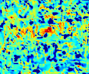
Now, with the key methodologies explained, we are ready to describe properties of the dynamically reconstructed eddies and their eddy forcing, and to compare them with those obtained for the locally filtered eddies. These properties are illustrated by figures 2 and 3. The resulting eddy forcing fields are characterised mostly by nearly grid-scale anomalies around the meandering eastward jet and most prominent vortices. This is expected, because the coarse-grid spatial derivatives have the largest errors on the steepest gradients, which characterise all these local flow features. The main difference between the upper- and deep-ocean eddy forcings is mostly in terms of their magnitudes, which tend to decrease with depth by one order of magnitude, from top to bottom. Analysis of the spatial structure of the dynamically reconstructed eddies (figure 2) reveals that although these eddies occupy the whole basin, their intensity is concentrated around the eastward jet, and this is even more so in the upper ocean. This behaviour is similar to that of the locally filtered eddies (figure 13 in Appendix B). We carried out formal evaluation of the involved dynamically reconstructed eddy scales from the spatial 2-D Fourier power spectra: the isotropic scales corresponding to the PV anomalies have the maximum power for the wavelengths of about 250 km (about eight coarse-grid intervals); the power spectrum is broad, with significant values (more than 10 % of the maximum power) occupying the wavelengths from 60 to 350 km (i.e. from 2 to 12 grid intervals).

Figure 2. Dynamically reconstructed eddy patterns. Instantaneous snapshots (a,d,g), time means (b,e,h) and standard deviations (c,f,i) for different upper-ocean eddy fields: (a–c) velocity streamfunction; (d–f) PVA; and (g–i) eddy forcing. Left column of panels illustrates the same time instance. All fields here and in the following figures are shown with the same non-dimensional units explained in figure 1.

Figure 3. Eigenvalues of the upper-ocean transport tensor obtained from the reduced fluxes of dynamically reconstructed eddies. Upper row of panels illustrates: (a) instantaneous snapshot, (b) time mean and (c) probability density function (PDF) of the signed logarithmic value of the largest eigenvalue ( $\lambda _1$). Lower row of panels illustrates the same but for the second (smaller) eigenvalue
  $\lambda _2$. The solid and dashed curves in (f) are reminiscent of the PDF in (c), for easier comparison.
To summarise, in this section we explained the methodology for obtaining the dynamically reconstructed eddies and illustrated the eddies themselves. The main part of the eddy feedback onto the large scales is divergence of the layer-wise eddy-induced flux  ${\boldsymbol f}$,
 \begin{equation} \boldsymbol{\nabla} \boldsymbol{\cdot} {\boldsymbol f} =\boldsymbol{\nabla} \boldsymbol{\cdot} ( \bar{\boldsymbol u} q' +{\boldsymbol u'} \bar{q} +{\boldsymbol u'} q') ,\end{equation}
and the rest of the analyses will be based on translating this flux into the corresponding layer-wise transport tensor  ${\boldsymbol K}$, with follow-up physical interpretations.
4. Transport tensor analysis
Working with the full eddy fluxes is a legitimate option (Bachman, Fox-Kemper & Bryan Reference Bachman, Fox-Kemper and Bryan2015, Reference Bachman, Fox-Kemper and Bryan2020), however, the rotational part of the flux typically dominates the divergent part by 1–2 orders of magnitude (Marshall & Shutts Reference Marshall and Shutts1981), which is also confirmed in our study. The divergent flux is obtained by using Helmholtz decomposition (Lau & Wallace Reference Lau and Wallace1979), which decomposes a vector field into its rotational, divergent and harmonic components. For this reason, we proceed with the divergent eddy flux  ${\boldsymbol f}_{div}$ by inverting the Poisson equation. Here
  $\nabla ^2\phi =\boldsymbol {\nabla } \boldsymbol {\cdot } {\boldsymbol f}$, with imposed zero normal-flux boundary condition (Maddison, Marshall & Shipton Reference Maddison, Marshall and Shipton2015) for the divergent potential
  $\phi$. The inversion problem is solved by the Fourier analysis and cyclic reduction method (Swarztrauber Reference Swarztrauber1974). We then set
  ${\boldsymbol f}_{div}=\boldsymbol {\nabla } \phi$, which, for brevity, we will refer to as the (reduced) eddy flux. Nevertheless, properties of the transport tensor obtained for the full flux have their own value for several reasons, therefore, they are presented and discussed in Appendix A.
The transport tensor  ${\boldsymbol K}$ can be found by solving the flux-gradient relation,
 \begin{equation} {\boldsymbol f}_{div}={-}{\boldsymbol K} \boldsymbol{\nabla} \bar{q}\end{equation}
for each isopycnal layer and spatial location (i.e. grid point), but note that this vector equation is equivalent to two scalar equations (for each flux component), whereas  ${\boldsymbol K}$ has four unknowns. One way to overcome this problem is by using two independent tracers, and, in principle, we can add one passive tracer and combine its flux-gradient relation with the above one for the eddy PV flux and
  $\bar {q}$, assuming the same
  ${\boldsymbol K}$. Although, this approach is legitimate, it results in different
  ${\boldsymbol K}$ for different tracer pairs. This fundamental non-uniqueness problem is thoroughly discussed in Sun et al. (Reference Sun, Haigh, Shevchenko, Berloff and Kamenkovich2021), but its implications are not yet properly understood. Here, we avoid using extra tracer and overcome the problem by considering the following additional constraint. First, we diagnose separately both relative-vorticity and buoyancy eddy fluxes,
 \begin{equation} {\boldsymbol f}_{\zeta}=\bar{\boldsymbol u} \zeta' +{\boldsymbol u'} \bar{\zeta} +{\boldsymbol u'} \zeta' , \quad {\boldsymbol f}_b=\bar{\boldsymbol u} b' +{\boldsymbol u'} \bar{b} +{\boldsymbol u'} b' ,\end{equation}
where the layer index is omitted for simplicity, and both fluxes are assumed to be reduced to their divergent components. Second, we assume that each flux satisfies its own flux-gradient relation with the same  ${\boldsymbol K}$,
 \begin{equation} {\boldsymbol f}_{\zeta}={-}{\boldsymbol K} \boldsymbol{\nabla} \bar{\zeta} , \quad {\boldsymbol f}_b={-}{\boldsymbol K} \boldsymbol{\nabla} \bar{b} .\end{equation}
Note that the corresponding flux-gradient relation for PV follows from the above relations automatically and with the same transport tensor. It is worth noting that the same decomposition can be carried out for a three-dimensional (3-D) model instead of layered 2-D model considered here; however, in the 3-D case the antisymmetric tensor is associated only with the vertical streamfunction (Griffies Reference Griffies1998; Bachman & Fox-Kemper Reference Bachman and Fox-Kemper2013; Bachman et al. Reference Bachman, Fox-Kemper and Bryan2015, Reference Bachman, Fox-Kemper and Bryan2020).
The layer-wise maps of transport tensor  ${\boldsymbol K}$ are systematically decomposed into their diffusive (symmetric) and advective (antisymmetric) components according to (1.2),
 \begin{equation} {\boldsymbol S}=\frac{1}{2} ({\boldsymbol K}+{\boldsymbol K}^T) , \quad {\boldsymbol A}=\frac{1}{2} ({\boldsymbol K}-{\boldsymbol K}^T) =\left[ \begin{matrix} 0 & A \\ -A & 0 \end{matrix} \right] .\end{equation}
The  ${\boldsymbol A}$-tensor represents advection of the large-scale dynamical tracers by a non-divergent (i.e. solenoidal) eddy-induced velocity
  ${\boldsymbol v}^*=(-\partial A/\partial y, \partial A/\partial x)$. Since the diffusion
  ${\boldsymbol S}$-tensor is real and symmetric, it has real eigenvalues
  $\lambda _1$ and
  $\lambda _2$ that represent local diffusivities in the directions of their respective local eigenvectors. We obtain these eigenvalues by rotating the coordinate system through diffusion angle
 \begin{equation} \alpha =\frac{1}{2} \tan^{{-}1} \left( \frac{2 S_{12}}{S_{11}-S_{22}} \right) ,\end{equation}
which is a fundamental local property of  ${\boldsymbol S}$, chosen so to correspond to the eigenvector of the largest eigenvalue, always denoted as
  $\lambda _1$. The diagonalised matrix
  ${\boldsymbol S}'$ is obtained by the rotation defined via rotation matrix
  ${\boldsymbol R}$,
 \begin{equation} {\boldsymbol S}'={\boldsymbol R}^T {\boldsymbol S} {\boldsymbol R}= \left[ \begin{matrix} \lambda_1 & 0 \\ 0 & \lambda_2 \end{matrix} \right] , \quad {\boldsymbol R}= \left[ \begin{matrix} \cos\alpha & -\sin\alpha \\ \sin\alpha & \cos\alpha \end{matrix} \right] ,\end{equation}
so that the eigenvalues can be expressed as
 \begin{gather} \lambda_1 =S_{11} \cos^2\alpha +S_{22} \sin^2\alpha +2 S_{12} \sin\alpha \cos\alpha , \end{gather}
 \begin{gather}\lambda_2 =S_{11} \sin^2\alpha +S_{22} \cos^2\alpha -2 S_{12} \sin\alpha \cos\alpha . \end{gather}
We deal with the eigenvalues individually but also discuss both the isotropic and deviatoric  ${\boldsymbol S}$-tensor components, which are denoted as
  $T$ and
  $\varPi$, respectively, so that
 \begin{equation} {\boldsymbol S}=T \left[ \begin{matrix} 1 & 0 \\ 0 & 1 \end{matrix} \right] +\varPi \left[ \begin{matrix} 1 & 0 \\ 0 & -1 \end{matrix} \right] .\end{equation}
Note that  $T$ can be interpreted as isotropic diffusivity and have either sign, whereas
  $\varPi$ is purely anisotropic filamentation (i.e. negative diffusivity in one direction and positive diffusivity of the same strength but in the transverse direction), which is positively defined because
  $\lambda _1 \ge \lambda _2$. In the
  ${\boldsymbol A}$-tensor we consider the only element
  $-A$, which can be interpreted as the eddy-induced velocity streamfunction. Since properly signed derivatives of the streamfunction are velocity components, we focus our analyses on the eddy-induced velocity speed
  $|\boldsymbol {\nabla } A|$, which becomes the third fundamental characteristics in addition to
  $T$ and
  $\varPi$. Note that this property is non-zero for spatially inhomogeneous eddy-induced transports, which is here the case.
The eigenvalues of the  ${\boldsymbol S}$-tensor (figure 3) are predominantly polar, which is an important result obtained here for the first time for active tracers and from the brute-force estimation of the full transport tensor. Note that it is unusual to deal simultaneously with both positive and negative eddy diffusion (of density) and viscosity (of momentum); more on that side can be found in Haigh & Berloff (Reference Haigh and Berloff2021, Reference Haigh and Berloff2022) analyses of passive tracers. Firstly, by construction, our transport tensor is the same for the involved dynamical properties – PV, relative-vorticity (i.e. momentum) and isopycnal thickness (i.e. density anomaly). Secondly, our
  ${\boldsymbol K}$-tensor is not constrained to be only some
  ${\boldsymbol S}$-tensor, hence, eddy diffusion (with any sign of diffusivity involved) is not the only physical process induced by the eddies. Thirdly, we allow the eigenvalues to be of any sign and different from each other, by not imposing any additional constraints. Therefore, we can recover genuine eddy effects acting with (positive) diffusion in one direction and with (negative) anti-diffusion in the direction transverse to it – this mixes up both processes in a fundamentally co-existing manner. The leading eigenvalue
  $\lambda _1$ is typically positive, whereas the second eigenvalue
  $\lambda _2$ is typically negative; however, sometimes both local eigenvalues can be of the same (either) sign, which then indeed corresponds to the local 2-D diffusion or anti-diffusion. The time-mean eigenvalues are clearly polar, and the basin average of the leading one has slightly larger magnitude, which implies that within the co-existing processes diffusion slightly prevails over anti-diffusion. Overall, similar qualitative conclusions are drawn from analyses of the deep-ocean layers, but we omitted them for brevity.
It is useful to look at the ratio of eigenvalues in terms of its diagnosed probability (figure 4), that succinctly describes anisotropy of the eddy-induced diffusion process. The positive ratio is mostly due to both eigenvalues being positive (and having both negative rarely happens), but the histogram shows that this relatively rarely happens; furthermore, there is a probability gap for the unity ratio suggesting that the isotropic diffusivity situation is exceptionally rare. On the other hand, the polar situation with the negative eigenvalue dominating over the positive one is very common (range of values from  $-1$ to zero in figure 4). Comparison of this ratio distribution with the one found for full fluxes (see Appendix A for a full-flux analysis) shows that the flux reduction noticeably reduces frequency of situations with a dominant negative eigenvalue, as well as creates the frequency peak at
  $-1$ (pure filamentation) and the frequency gap at
  $+1$ (pure isotropic diffusion). These features appear as numerical consequences of the Helmholtz decomposition. Overall, the eigenvalue ratio distributions are found similar for the locally filtered eddies (Appendix B).

Figure 4. Histogram of the diffusion anisotropy, equal to the ratio of the eigenvalues  $\lambda _1/\lambda _2$, for the dynamically reconstructed eddies for the reduced fluxes. Negative ratio implies polarity of the eigenvalues, and when it is also bigger than
  $-1$, the negative eigenvalue dominates. Contributions of different intervals are shown on the panel.
The eigendirections, that is, spatial directions of diffusion and (transverse to it) antidiffusion are highly transient and vary in accord with temporal correlations imposed by the eddies, as well as they vary spatially. This process is conveniently described by spatio-temporal variability of the diffusion angle  $\alpha$ given by (4.5) and illustrated by figure 5. Note that the probability density function (PDF) of
  $\alpha$, which by definition belongs to
  $(-{\rm \pi} /2, {\rm \pi}/2]$, has two narrow peaks corresponding to
  $\pm {\rm \pi}/4$. These values are tied to the orientation of the coarse grid and have purely numerical discretisation origin, thus underlying the fact that numerical aspects are built into the reconstruction of dynamical eddies. The domain-averaged autocorrelation function (figure 4c) decays out quickly (over a few days) and without noticeable oscillations. This is in a way good news indicating that, in a stochastic parameterization of transport tensor, the diffusion angle can be simulated as a simple first-order autoregressive process with exponential autocorrelation roll-off.

Figure 5. Statistics of the diffusion angle  $\alpha$ of the upper-ocean transport tensor obtained from the reduced fluxes of dynamically reconstructed eddies. Shown are: (a) instantaneous snapshot and (b) PDF of
  $\alpha$. The time-mean field is close to zero and not shown. (c) Local temporal autocorrelation functions of the diffusion angle (time lag is in days). Grey curves correspond to 100 evenly distributed grid points in the domain; the bold curve is the domain-averaged (over
  $129\times 129$ grid points) autocorrelation function.
Fundamental transport tensor properties to be discussed now provide the most substantial information on effects of the dynamically reconstructed eddies (figure 6), which are the upper-bound target for parameterizations. The isotropic diffusivity  $T$ is characterised by a double-hump log-scale PDF, with roughly half of the values being negative and the other half being positive. The positive hump is only slightly bigger, therefore, the time-mean and basin-averaged value of
  $T$ is positive but very small. Since
  $T$ is a signed quantity, looking directly at its raw PDF is also informative (figure 7). This PDF is symmetrically centred on a very small positive value and is characterised by heavy tails and a sharp peak at zero, all succinctly quantified by the large value of kurtosis (nearly 2). In terms of dimensional values, the mean
  $T$ is about 200 m
 $^2$ s
 $^{-1}$, whereas the standard deviation is about
  $10^4$ m
 $^2$ s
 $^{-1}$. The latter value is broadly consistent with various diffusivity estimates from observations and models (Eden & Greatbatch Reference Eden and Greatbatch2009; Rypina et al. Reference Rypina, Kamenkovich, Berloff and Pratt2012; Zhurbas, Lyzhkov & Kuzmina Reference Zhurbas, Lyzhkov and Kuzmina2014; Haigh et al. Reference Haigh, Sun, Shevchenko and Berloff2020). The spatial distribution of
  $T$ is nearly homogeneous with slightly larger values in the broadly defined eastward jet region. These properties of the isotropic diffusivity show that it can not be approximated either by some constant value or by some time-independent spatial field; instead, it should be treated in terms of co-existing and spatially inhomogeneous, positive and negative diffusivity eigenvalues. Finally, we checked whether
  $T$ and
  $\varPi$ have any empirical functional relation with each other, that is, whether larger magnitudes of
  $T$ correspond to larger values of
  $\varPi$. Scatterplots between these properties showed broad distributions with no visible relation, thus suggesting their independence from each other.

Figure 6. Transport tensor properties from the upper-ocean reduced fluxes of dynamically reconstructed eddies. Upper row: isotropic component  $T$ of the diffusion tensor. Middle row: deviatorical component
  $|\varPi |$ of the diffusion tensor. Bottom row: advection tensor presented as the eddy-induced speed
  $|\boldsymbol {\nabla } A|$. All fields are plotted with a signed natural logarithmic scale. Left column of panels, instantaneous snapshots; middle column, time means; right column, PDFs. Since
  $T$ is signed characteristic, panel (c) shows two PDFs, plotted separately for the corresponding positive and negative values. Solid curves in panels (f) and (i) remind of the right bell-shaped PDF component from panel (c); dashed curve in panel (i) is reminiscent of the PDF from panel (f), all for the ease of comparison. The shapes of the histograms from the upper panels are shown by the solid and dashed curves. The units are the same across all fields:
  $3 \times 10^2$ m
 $^2$ s
 $^{-1}$.

Figure 7. Probability density function of the signed characteristic  $T$ (see figure 6(c) for the logarithm-scaled representation). Moments of the PDF are indicated (note that kurtosis is defined to be zero for the normal distribution). The statistics are calculated for the shown range of non-dimensional values
  $[-100, 100]$.
Now, let us discuss the results on anisotropic filamentation  $\varPi$ and eddy-induced speed
  $|\boldsymbol {\nabla } A|$ (figure 6). Firstly, typical values of
  $\varPi$ are significantly (by order of magnitude) larger than those of
  $T$, which is a surprising result by itself. Secondly, values of
  $\varPi$ are also highly transient and broadly distributed, thus precluding its potential approximation as a constant or as a stationary spatial map. Thirdly, large values of
  $\varPi$ tend to be concentrated in the broad eastward jet region and near the meridional boundaries, thus contrasting a lot more uniform distribution of
  $T$. The eddy-induced speed shares the same properties with
  $\varPi$ (except that its PDF is slightly broader), therefore, we concluded that these two properties are the most important characteristics of the transport tensor estimated in the paper, whereas the isotropic diffusivity is of secondary importance.
The last analyses are separate comparisons of the reference transport tensor properties with those obtained for the full eddy fluxes and locally filtered eddies. In the past, analysis of transport tensors for passive tracers showed that they are significantly different between reduced and full eddy fluxes (Sun et al. Reference Sun, Haigh, Shevchenko, Berloff and Kamenkovich2021). Whether this is true for the dynamical tracers considered here remains to be checked. Also, past analyses showed that dynamically reconstructed and locally filtered eddies are significantly different (Berloff et al. Reference Berloff, Ryzhov and Shevchenko2021), but how these differences are translated into the transport tensors for the dynamically active tracers also remains to be found. Appendices A and B deal with these issues, and the summary of their outcomes is the following. In comparison with the reference case,  ${\boldsymbol K}$-tensors estimated from the full fluxes and locally filtered eddies have both similar and dissimilar properties. The former ones are the discovered polarity of the eigenvalues and the surprising dominance of the filamentation and advection processes, that is, all the main qualitative aspects. The latter ones are the increased polarity of the eigenvalues, the larger values of all
  ${\boldsymbol K}$-tensor components (nearly by order of magnitude), and the longer tails of the probabilistic distribution of
  $T$. As for
  ${\boldsymbol K}$-tensor estimated from the locally filtered eddies, its differences from the reference case are even more significant. Not only the magnitude of the
  ${\boldsymbol K}$-tensor elements becomes 3–4 times larger, but also their spatial distributions change significantly and become more localised around the eastward jet core, as well as they extend significantly more to the east.
Now, let us add one more interpretation level of the results and investigate the importance of the spatial inhomogeneities of  $T$ and
  $\varPi$, while keeping in mind that spatial inhomogeneity of
  $A$ is absolutely crucial, as without it the advective eddy effect is absent. For this purpose, we locally rotate back by
  $-\alpha$ decomposition (4.9), so that it can be dealt with as the spatial map and, therefore, can be straightforwardly differentiated in space. In this case the isotropic part does not change, therefore, the filamentation part can be simply written as
 \begin{equation} {\boldsymbol \varPi} \equiv \left[ \begin{matrix} \varPi_{11} & \varPi_{12} \\ \varPi_{12} & \varPi_{22} \end{matrix} \right] \equiv \left[ \begin{matrix} S_{11}-T & S_{12} \\ S_{12} & S_{22}-T \end{matrix} \right] = \varPi \left[ \begin{matrix} \cos{2\alpha} & \sin{2\alpha} \\ \sin{2\alpha} & -\cos{2\alpha} \end{matrix} \right] ,\end{equation}
where the last expression is obtained by rotating back the filamentation matrix in (4.9). When  ${\boldsymbol K}$ is substituted into the flux-gradient relation, the eddy flux divergence can be written as
 \begin{equation} \boldsymbol{\nabla} \boldsymbol{\cdot} {\boldsymbol f}_{div}={-}T \nabla^2 \bar{q} -\varPi_{11} \frac{\partial^2 \bar{q}}{\partial x^2} -\varPi_{22} \frac{\partial^2 \bar{q}}{\partial y^2} -2 \varPi_{12} \frac{\partial^2 \bar{q}}{\partial x \partial y} +{\boldsymbol U}^* \boldsymbol{\cdot} \boldsymbol{\nabla} \bar{q} ,\end{equation}
where the first term is isotropic diffusion; the last advective term is in our focus and will be explained and analysed below; and the middle group representing the filamentation has no derivatives of the elements of  ${\boldsymbol \varPi }$. In the rotated local coordinates, this group can be written as
  $-\varPi (\partial ^2 \bar {q}/\partial X^2 -\partial ^2 \bar {q}/\partial Y^2 )$, where
  $X$ and
  $Y$ indicate local coordinates along the first (major) and second (minor) eigendirections, respectively. Thus, if the large-scale field curvatures along these directions are equal, then this part of filamentation does not contribute to the flux divergence, hence, to the eddy forcing. The total eddy-induced velocity is
 \begin{equation} {\boldsymbol U}^* ={\boldsymbol U}^A +{\boldsymbol U}^T +{\boldsymbol U}^{\varPi} , \end{equation}
where it is naturally split into the following three components:
 \begin{align} {\boldsymbol U}^A &=\left(\frac{\partial A}{\partial y}, -\frac{\partial A}{\partial x} \right) , \quad {\boldsymbol U}^T ={-}\left(\frac{\partial T}{\partial x}, \frac{\partial T}{\partial y} \right),\nonumber\\ {\boldsymbol U}^{\varPi}&={-}\left(\frac{\partial \varPi_{11}}{\partial x}+\frac{\partial \varPi_{12}}{\partial y}, \frac{\partial \varPi_{12}}{\partial x}+\frac{\partial \varPi_{22}}{\partial y} \right). \end{align}
We already encountered the first component, when we considered the eddy-induced speed  $|\boldsymbol {\nabla } A|$. The upcoming statement that spatial inhomogeneities of
  $T$ and
  ${\boldsymbol \varPi }$ are important or not translates into importance of
  ${\boldsymbol U}^T$ and
  ${\boldsymbol U}^{\varPi }$ relative to
  ${\boldsymbol U}^A$, and into importance of the (last) advective term in (4.11) relative to the other right-hand side terms. Firstly, we found that all terms involving
  $T$ are relatively small and, therefore, unimportant, which is consistent with the earlier analyses of the transport tensor components. The first right-hand side term in (4.11) is relatively small as well;
  $|{\boldsymbol U}^T| \ll |{\boldsymbol U}^A+{\boldsymbol U}^{\varPi }|$, and the angle between
  ${\boldsymbol U}^T$ and
  ${\boldsymbol U}^A+{\boldsymbol U}^{\varPi }$ is broadly distributed, thus indicating no prevalent orientation of
  ${\boldsymbol U}^T$. We also compared
  ${\boldsymbol U}^A$ and
  ${\boldsymbol U}^{\varPi }$ and found that the latter dominates in terms of magnitude. This is because
  ${\boldsymbol U}^{\varPi }$ is differentiated out of
  ${\boldsymbol \varPi }$, which in turn has a magnitude similar to
  $|{\boldsymbol U}^A|$. This ordering of the relative importance of the corresponding velocity fields is also evident from their energy content. The total energy is concentrated in
  $U^A$ and
  $U^\varPi$, while
  $U^T$ is two orders of magnitude weaker (figure 8). The angle between these velocities is broadly distributed, but the probability significantly decreases with it, thus indicating that these velocities tend to be aligned and enhance rather than compensate each other. To summarise, from these analyses we conclude that spatial inhomogeneities of
  $A$ and
  $\varPi$ are important and cannot be neglected in parameterizations, and the inhomogeneity of the latter, that is, of the filamentation process, is the most important aspect.

Figure 8. Logarithmically scaled domain-averaged energy content associated with the corresponding velocity components from (4.12). The series are smoothed using a 500-day moving averaging. The ordering of the relative importance of the tensor components remains the same as argued, with  $U^T$ being the weakest one.
Finally, we ask the question on how the divergent eddy fluxes contribute to the large-scale enstrophy  ${\bar q}^2/2$ budget and production. Purely diffusive processes (overall) transfer enstrophy away from the large scales and into the small scales, but in the situation with polar eigenvalues this is not generally guaranteed, and our goal is to detail the process. A similar precursor study focusing on passive tracers is by Haigh & Berloff (Reference Haigh and Berloff2021), but the novelty here is not only in terms of active tracers but also in terms of analysing the dynamically consistent eddies. The large-scale enstrophy equation is obtained by multiplying (3.4) with
  $\bar q$, by rearranging the terms and considering only contribution from the eddy flux,
 \begin{equation} -{\bar q} \boldsymbol{\nabla} \boldsymbol{\cdot}{\boldsymbol f}_{div} ={-}\boldsymbol{\nabla} \boldsymbol{\cdot} ({\bar q} {\boldsymbol f}_{div}) +{\boldsymbol f}_{div} \boldsymbol{\cdot} \boldsymbol{\nabla} {\bar q}.\end{equation}
The first term on the right-hand side is flux divergence, whereas the second term is production of enstrophy due to alignment between the divergent eddy flux and large-scale PVA gradient. This term can be further decomposed into enstrophy productions due to the buoyancy and relative-vorticity fluxes, respectively,
 \begin{equation} P^b ={\boldsymbol f}_{b} \boldsymbol{\cdot} \boldsymbol{\nabla} \bar{q} , \quad P^{\zeta} ={\boldsymbol f}_{\zeta} \boldsymbol{\cdot} \boldsymbol{\nabla} \bar{q} , \end{equation}
and spatial distribution of these terms is illustrated in figure 9. The main conclusion about them is that their standard deviations are similar, and instantaneous patterns are both complex and characterised by anomalies of either sign populating the eastward jet region. The main physical message, though, comes from the enstrophy production time-mean fields, which have opposite signs in the eastward jet region. Here,  $P^b$ is predominantly negative, thus indicating that the eddy buoyancy effects are on average diffusive (i.e. corresponding to positive diffusivity), whereas,
  $P^{\zeta }$ is predominantly positive, thus indicating that the eddy momentum effects are on average negative (i.e. corresponding to negative viscosity). Overall, the former effect is a few times stronger than the latter, which brings up an interesting alignment and comparison with a recent comprehensive ocean modelling study by Shevchenko & Berloff (Reference Shevchenko and Berloff2021b), who argue that missing eddy effects in the thermodynamics are significantly more important than those in the momentum equation. Appendix B shows that the enstrophy productions for the locally filtered eddies are a few times weaker and are also fundamentally different, because they both consist of anomalies with different signs and cannot be characterised as a single-sign diffusion or viscosity.

Figure 9. The statistics of the buoyancy and relative-vorticity enstrophy transfer from the dynamically reconstructed eddies to the large scales.
5. Conclusions and discussion
This paper was motivated by the necessity to parameterize effects of mesoscale oceanic eddies in non-eddy-resolving and eddy-permitting OGCMs. Searching for suitable and accurate eddy parameterizations is both a challenging task and an active research direction, which is rife with many new and interesting ideas. The main problems facing researchers can be summarised (also, ranked in terms of their descending importance) as follows: (i) defining eddies (hence their effects) in a way that is consistent with the coarse-grid dynamics employed to model the large-scale circulation and to host the corresponding parameterization of the unresolved eddy effects; (ii) finding a suitable mathematical model for representing the eddy effects; (iii) relating parameters of the chosen mathematical model to the explicitly resolved large-scale circulation properties. Our paper deals with (i) and focuses on exploring dynamical properties of eddies defined in a novel way, which is arguably the most suitable for parameterization. We also deliberately stay within the framework of parameterizations based on turbulent diffusion, and more broadly and importantly on the fundamental flux-gradient relation, while recognising the importance of the alternative approaches (§ 1). For interpreting the corresponding dynamical eddy effects, we applied a new approach that is based on estimating the full eddy-induced transport tensor and its components. Analysis of the transport tensor uncovered the relative importance of different and underestimated physical processes and, thus, it provides a guidance on what exactly should be targeted by eddy parameterizations.
For the main set-up, we considered an idealised double-gyre QG ocean circulation model with a coarse (eddy-permitting) spatial grid resolution on the one hand, and with the reference ocean circulation field provided by the HR model configuration, on the other hand. The latter has been obtained by solving exactly the same idealised ocean model but with sufficiently fine grid resolution, so that the eddy effects were directly and completely taken into account. The corresponding solution was projected on the coarse grid to become the reference flow field; note that, for our analyses, the reference flow could come from observations, and only for the lack of those we are to deal with a model solution. Next, with our novel procedure the coarse-grid model was used explicitly to reconstruct the dynamical eddies, which rigorously and exactly – when taken into account – augment solution of the coarse-grid model towards the reference flow field. Within each isopycnal layer of the model, we found space–time history of the dynamically reconstructed eddies, as well as the corresponding eddy fluxes of PV, relative vorticity and buoyancy. Via the corresponding flux-gradient relations, these fluxes were translated into the space–time history of the unique transport tensor  ${\boldsymbol K}$, including its symmetric
  ${\boldsymbol S}$ and antisymmetric
  ${\boldsymbol A}$ components. We forced
  ${\boldsymbol K}$ to be unique by constraining it to be the same for the relative-vorticity (i.e. momentum) and buoyancy (i.e. isopycnal thickness) PV components; then, it becomes the same for the PV itself.
From the transport tensor analysis, we found that the advective (non-diffusive) tensor component  $A$ is significant and, therefore, it must be taken into account by eddy parameterizations. Note that the
  $A$-component is usually neglected (e.g. as in purely diffusive parameterizations), but here, due to its spatial inhomogeneities, it significantly (as we have found) affects the large-scale circulation via the resulting divergence of the corresponding eddy fluxes. We also found that the diffusive part of the transport tensor is characterised by the eigenvalues that are predominantly polar, that is, have opposite signs – this is a new result for active tracers, although it has been anticipated by recent results for passive tracers (Haigh & Berloff Reference Haigh and Berloff2021; Haigh et al. Reference Haigh, Sun, McWilliams and Berloff2021a). Physically, this means that most commonly positive diffusivity in one direction is accompanied by negative diffusivity in the transverse direction, and roughly half of the space–time probability corresponds to the negative diffusivity having the larger magnitude. Studies of polar diffusion eigenvalues and negative diffusivities are scarce, since simulations with diffusive parameterizations involving negative diffusivities are susceptible to instabilities (Haigh & Berloff Reference Haigh and Berloff2021). With that study as a precursor, our results imply that using polar diffusivities is fully justified and may be even required for accurate parameterizations. In this case, instabilities may be mitigated by such factors as rotation of the diffusion angle, transience of the eigenvalues, large-scale advection and explicit (positive) diffusion introduced as an additional parameterization.
We analysed the  ${\boldsymbol S}$-tensor in terms of its isotropic
  $T$ and filamentation
  $\varPi$ components, respectively. The former is characterised by unit eigenvalues, hence, it has no preferred spatial direction; whereas the latter has opposite-signed eigenvalues of the same magnitude and aligned with eigendirections of diagonalised
  ${\boldsymbol S}$. Generally it is optimistically believed that the isotropic part can dominate, hence, the transport tensor can be simpler approximated by a scalar field. However, our results dispel this optimism and demonstrate that
  $\varPi$ completely dominates over
  $T$ and is of similar magnitude to
  $A$. Furthermore, we inquired whether spatial inhomogeneities of
  $T$ and
  $\varPi$, which can be interpreted as eddy-induced velocities, are as important as those corresponding to
  $A$, hoping that their hypothetical unimportance can help to simplify representation of the transport tensor for practical parameterizations. This optimistic hypothesis was turned down as well, as we found that spatial inhomogeneities of
  $\varPi$ are significant and also, most importantly, even more important than those of
  $A$, and also both of the
  $T$ and
  $\varPi$ effects tend to reinforce each other. On the positive side, the spatial inhomogeneities of
  $T$ were found to be relatively negligible.
Our results explored the transport tensor properties based on the eddy fluxes reduced to their divergent component, so that the rotational fluxes were filtered out. On the one hand, since the eddy forcing is equal to convergence of the eddy fluxes, the rotational flux component does not contribute to it and can be removed. However, this removal changes the transport tensor, which is in the focus of our story, and these changes are to be reported and understood. We found that the flux reduction significantly reduces all elements and parts of the transport tensor, but retains the prevailing polarity of the eigenvalues and relative importance of different components. It also shifts the probability peaks in the statistical distribution of the diffusion angle from zero and  ${\rm \pi} /2$ to
  $\pm {\rm \pi}/4$, which is a numerical effect imposed by the employed regular Cartesian grid. Also the reduction of the eddy fluxes significantly reduces the probability of instances when the negative eigenvalue dominates over the positive one. To summarize, the flux reduction just yields a different but smaller-sized transport tensor, without changing its most important properties to deal with.
Finally, we compared all these findings with those for the common, locally filtered (by convolution with a box-car filter) eddies, and showed that the latter outcome is different in several aspects. First, all the elements and components of the transport tensor became 3–4 times larger, despite choosing such a filter size that the total time-mean energies of the dynamical and locally filtered eddies are nearly the same. From this we concluded that the dynamical action of the locally filtered eddies is similar, but their eddy-induced transports are significantly less efficient. Second, the diffusion tensor for the locally filtered eddies exhibits more significant preference to be zonally oriented, and we explain this by the fact that the locally filtered eddies are in general more anisotropic and zonally elongated (Kamenkovich, Rypina & Berloff Reference Kamenkovich, Rypina and Berloff2015). Third, the spatial pattern of the locally filtered transport tensor is noticeably different: it is more aligned with the eastward jet and extends along it farther to the east; also, all elements of  ${\boldsymbol K}$ are significantly reduced near the western boundary. This comparison proves that the dynamically reconstructed eddies not only profoundly differ in terms of their statistical properties (Berloff et al. Reference Berloff, Ryzhov and Shevchenko2021), but also differ in terms of their dynamical effects on the resolved large-scale circulation. Along this line, we also compared the buoyancy and relative-vorticity enstrophy production terms for both types of eddies and found the following fundamental difference. For the dynamically reconstructed eddies, the buoyancy effect is overall the positive diffusion in the key eastward jet region, and the relative-vorticity (i.e. momentum) effect is overall the negative viscosity. This is despite the eigenvalue polarity, which makes it difficult to extract the overall eddy effects. In contrast the locally filtered eddies show nothing like this, thus, they lack extra clarity and simplicity that should be useful for their parameterization. This suggests that one should expect significantly different parameterizations for these different eddy types, but the dynamically consistent eddies provide the upper bound for parameterizations, which is an obvious argument in their favour.
Let us now provide some critical assessment of our results. First, it is important to understand that dynamically reconstructed eddies provide the formal upper bound for all parameterizations. Aiming at the upper bound is not necessarily the best strategy for obtaining a useful practical parameterization and even for defining what needs to be parameterized. In principle, it may be more efficient to relax requirements for parameterization skills and still get significant model improvements – this is an important statement and here we basically throw it out into the ocean modelling (and beyond) community; clearly, more research needs to be carried out in this direction. Second, there may be some confusion about our definition of the mesoscale eddies, because they are not literally a physical object but rather they are formal field errors of the interactively augmented coarse-grid model. In other words, the dynamically reconstructed eddies are fundamentally (coarse-grid) model-dependent, but we argue that, for parameterization purposes, this is a desirable rather than negative property. This is because different models with different resolutions normally miss different eddy effects and, thus, no universal parameterization can be effectively employed to augment them. Third, in order to define the unique (recognising its non-uniqueness and dealing with it is also an option Sun et al. Reference Sun, Haigh, Shevchenko, Berloff and Kamenkovich2021) transport tensor, we assumed that it is the same for the relative-vorticity (i.e. momentum) and isopycnal-thickness (i.e. buoyancy) PV flux components, but in principle some other constraints may be implemented instead of what we have done. Despite all these issues, we argue that the dynamically reconstructed eddies are not only a legitimate but also the upper-bound target for parameterizations and, therefore, their analyses should be extended and deepened. To summarise, our results suggest enriching the most common eddy parameterization approach, which is based on fitting out a simplified eddy-induced diffusion process, by taking into account the full transport tensor approach in which the flux-gradient relation becomes genuinely fundamental and unconstrained for representing the eddy-induced fluxes.
We hope that, although our study deals with ocean circulation, the general idea of considering dynamically reconstructed eddies and translating their effects into the transport tensor may be useful for other areas of turbulence modelling. The reported results prompt several future extensions. First, an extension of our study to the primitive equations, routinely used in oceanic GCMs, is anticipated as the most challenging but also the most rewarding further development. Second, we have to understand the relative importance of different components of the transport tensor for maintaining the time-mean state and large-scale variability of the ocean circulation. This will help understand possible biases and sensitivities to parameter uncertainties. A way to achieve this is by developing a skilled parameterized model, and by studying its prognostic, dynamical sensitivity to different elements of the parameterization – this would be a very challenging research program. Third, from the perspective of eddy backscatter processes (e.g. Jansen et al. Reference Jansen, Adcroft, Hallberg and Held2015, Reference Jansen, Adcroft, Khani and Kong2019; Shevchenko & Berloff Reference Shevchenko and Berloff2016; Klower et al. Reference Klower, Jansen, Claus, Greatbatch and Thomsen2018; Juricke et al. Reference Juricke, Danilov, Kutsenko and Oliver2019), it will be useful to study in more detail PV and energy inputs into the large-scale circulation from the eddy flux divergence, as well as from its components corresponding to specific components of the transport tensor. Fourth, so far the resolution of our employed QG ocean model is severely truncated in the vertical direction, which makes it harder to associate the obtained results with oceanic GCMs. Closing this gap by considering high vertical resolutions and the corresponding effects of the high baroclinic modes (Shevchenko & Berloff Reference Shevchenko and Berloff2017) will enhance our understanding of the dynamically reconstructed eddies and their effects. Fifth, looking for empirical statistical and physical relations between properties of the transport tensor and large-scale circulation may help to provide recipes for the ultimate parameterization closure; so far we left this story completely beyond the scope of the paper. Finally, anchoring eddy parameterization on the flux-gradient relation is not the only option, and extending and modifying this relation (e.g. by including the higher derivatives) is a promising avenue.
Declaration of interests
The authors report no conflict of interest.
Funding
E.A.R. was supported by the NERC grant NE/T002220/1 and Imperial CoA NERC grant. P.B. was supported by the NERC grants NE/R011567/1 and NE/T002220/1, and the Leverhulme grant RPG-2019-024. The part of the study conducted by E.A.R. that involved running the baroclinic QG model and analysing its eddying solutions was partly supported by the Russian Science Foundation (Project 19-17-00006). This study was also partially supported by POI FEB RAS Program ’Modelling of multi-scale dynamical processes in the ocean’, Russia (project no. 121021700341-2). P.B. was also supported by the Moscow Centre of Fundamental and Applied Mathematics (supported by the Agreement 075-15-2019-1624 with the Ministry of Education and Science of the Russian Federation).
Appendix A. Transport tensor properties: full fluxes
Here we address an important issue of ‘reducing’ layer-wise eddy fluxes by removing their non-divergent components and its effect on the resulting transport tensor. The rotational and harmonic flux components were obtained via the Helmholtz decomposition, as explained in the main text, and then removed from the flux. In this Appendix we do not reduce fluxes, that is, treat them as they are, find the corresponding transport tensors, study their properties and compare them with the reduced-flux ones obtained in the main text. What is the motivation for this analysis? First, the reduction procedure requires global knowledge of the eddy flux, and this may be unavailable from the observations. Second, for 3-D solutions of regional general circulation models with open boundaries, and also with complicated coastline and bottom topography, using our simple zero normal-flux boundary condition may become problematic. Third, inversion of the Poisson equation is a global problem, implying that local  ${\boldsymbol f}_{div}(t,{\boldsymbol x}$ and, hence, the local transport tensor depends on the far-field information. So far this dependence remains physically unjustified. Based on all this reasoning, considering eddy transport tensors based on full eddy fluxes is not only a legitimate but also, perhaps, more practical approach.
For brevity, we illustrate full-flux transport tensor properties in terms of the upper-ocean eigenvalues (figure 10) and fundamental composition given by  $T$,
$T$,  $|\varPi |$ and
  $|\boldsymbol {\nabla } A|$ (figure 11), although, all other characteristics were also looked at. The PDF of
  $T$ is not shown for brevity, because its shape is similar to the one in figure 7, and the corresponding mean, standard deviation and kurtosis are 1.6, 270 and 2.8, respectively, and skewness is zero.

Figure 10. Eigenvalues of the upper-ocean transport tensor obtained from the full fluxes of dynamically reconstructed eddies. Upper row of panels illustrates (a) instantaneous snapshot, (b) time mean and (c) PDF of the signed logarithmic value of the largest eigenvalue ( $\lambda _1$). Lower row of panels illustrates the same but for the second (smaller) eigenvalue
  $\lambda _2$. The solid and dashed curves in (f) remind of the PDF in (c), for easier comparison. This figure can be compared with figure 3, which illustrates eigenvalues obtained from the reduced fluxes.

Figure 11. The same as figure 6 but for the full eddy fluxes. Transport tensor properties from the upper-ocean full fluxes of dynamically reconstructed eddies. Upper row: isotropic component  $T$ of the diffusion tensor. Middle row: deviatorical component
  $|\varPi |$ of the diffusion tensor. Bottom row: advection tensor presented as the eddy-induced speed
  $|\boldsymbol {\nabla } A|$. All fields are plotted with a signed natural logarithmic scale. Left column of panels, Instantaneous snapshots; middle column, time means; right column, PDFs. Since
  $T$ is signed characteristic, panel (c) shows two PDFs, plotted separately for the corresponding positive and negative values. Solid curves in panels (f) and (i) remind of the right bell-shaped PDF component from panel (c); dashed curve in panel (i) is reminiscent of the PDF from panel (f), all for the ease of comparison. The shapes of the histograms from the upper panels are shown by the solid and dashed curves. The units are the same across all fields:
  $3 \times 10^2$ m
 $^2$ s
 $^{-1}$. This figure can be compared with figure 6, which illustrates transport tensor properties for the reduced eddy fluxes.
In comparison with the reference case, the  ${\boldsymbol K}$-tensor estimated from the full fluxes has both similar and dissimilar properties. Similarities are prevailing polarity of the eigenvalues, dominance of filamentation and advection over isotropic diffusion. The ratio of eigenvalues in terms of their diagnosed probabilities remains qualitatively similar, when full eddy fluxes are used (figure 5), but there is no peak/gap for
  $-1/+1$ values, and the total probability within the range
  $[-1,0]$ (negative
  $\lambda _2$ dominates) increases by about
  $20\,\%$. Dissimilarities are increased polarity of the eigenvalues (i.e. their absolute values are larger), larger values of all
  ${\boldsymbol K}$-tensor components (nearly by an order of magnitude) and longer tails of
  $T$ distribution. Narrow peaks of the diffusion angle migrate from
  $\pm {\rm \pi}/4$ to zero and
  ${\rm \pi} /2$ values (figure 12). This suggests that the angle PDF peaks for the reduced fluxes are dictated by the Helmholtz decomposition, which in turn is influenced by the numerical grid aligned both with the basin and geographical Cartesian coordinates. From this we conclude that the peaks are not important and rather are artefacts of the particular numerical discretisation.

Figure 12. Statistics of the diffusion angle  $\alpha$ of the upper-ocean transport tensor obtained from the full fluxes of dynamically reconstructed eddies. Shown are: (a) instantaneous snapshot and (b) PDF of
  $\alpha$. The time-mean field is close to zero and not shown.

Figure 13. Locally filtered eddy patterns. Instantaneous snapshots (a,d,g), time means (b,e,h) and standard deviations (c,f,i) for different upper-ocean eddy fields: (a–c) velocity streamfunction; (d–f) PVA; and (g–i) eddy forcing. Left column of panels illustrates the same time instance. This figure can be compared with figure 2, which illustrates dynamically reconstructed eddies.
Appendix B. Transport tensor properties: locally filtered eddies
Here we address an important issue which is understanding differences between transport tensors for dynamically reconstructed and locally filtered eddies. This paper is about the former case, but contrasting the outcome against a more common definition of eddies provides new knowledge about the physical mechanisms behind different eddy effects. Dynamical eddy reconstruction is (statistically) unique for a given coarse-grid model, but local eddy filtering is non-unique, because it depends on spatio-temporal characteristics of the filter. This makes comparison between the two eddy types rather problematic. Here, we restrict our local filtering to the most simple (other alternatives may be correlation-based or spectral filtering approaches Agarwal et al. Reference Agarwal, Ryzhov, Kondrashov and Berloff2021), spatial one based on running square-box averaging. Within this framework the only control parameter is the filter width. We chose it such that the total eddy energy is roughly equal to that of the dynamically reconstructed eddies. This resulted in the filter width (near the basin boundaries the filtering width was reduced, so that it remained always twice the distance to the nearest boundary point) of 280 km, which corresponds to  $w=45$ in (3.1) of the HR grid and to the length of 7.0 first Rossby baroclinic radii. We also varied
  $w$ by
  $\pm 30\,\%$ and recovered qualitatively similar results, not discussed here for the sake of brevity. The filtering is applied to PVA fields of the reference solution already projected on the coarse grid, and the corresponding velocity streamfunction is inverted out.
After filtering, the locally filtered eddies are obtained as the residual, according to (3.2), and the outcome is illustrated by figure 13. The locally filtered eddies are qualitatively and profoundly different from the dynamically reconstructed ones, because they have a robustly present ribbon-like feature that straddles the eastward jet and contains PVAs of the same polarity as the nonlinear recirculation zones adjacent to it. These ribbons are due to the smoothing effect of the filtering on the sharp PV gradient corresponding to the eastward jet core. Intensity of the locally filtered eddies and their eddy forcing is more localised around the eastward jet core, and the time-mean fields are more pronounced. How are all these differences translated into the transport tensor differences?
The transport tensor fields based on the reduced eddy fluxes were processed with the same methodology as for the main results. For brevity, we illustrate  ${\boldsymbol K}$-tensor properties in terms of the upper-ocean eigenvalues (figure 14) and fundamental composition given by
  $T$,
$T$,  $|\varPi |$ and
  $|\boldsymbol {\nabla } A|$ (figure 15), although, all the other characteristics were also looked at. The magnitude of the
  ${\boldsymbol K}$-tensor elements became 3–4 times larger, and their spatial distribution changed significantly and became more localised around the eastward jet core and more extended to the east. On the other hand, near the western boundary polarity of the eigenvalues reduced significantly, thus resulting in small values of
  $\varPi$, and this is also accompanied by a similar reduction of the advective velocity. The distribution of
  $T$ became more heavy tailed, as expressed by kurtosis values increasing to more than 8, and standard deviation increased by a factor of six. If the eddy fluxes are not reduced, then kurtosis becomes about twice smaller and standard deviation about twice larger. The ratios of eigenvalues in terms of their diagnosed probabilities are remarkably similar to those obtained both for reduced (figure 5) and full (not shown) dynamical eddy fluxes.

Figure 14. The same as figure 3 but for the locally filtered eddies. Eigenvalues of the upper-ocean transport tensor obtained from the reduced fluxes of locally filtered eddies. Upper row of panels illustrates (a) instantaneous snapshot, (b) time mean and (c) PDF of the signed logarithmic value of the largest eigenvalue ( $\lambda _1$). Lower row of panels illustrates the same but for the second (smaller) eigenvalue
  $\lambda _2$. The solid and dashed curves in (f) remind of the PDF in (c), for easier comparison.

Figure 15. The same as figure 6 but for the locally filtered eddies. Transport tensor properties from the upper-ocean reduced fluxes of locally filtered eddies. Upper row: isotropic component  $T$ of the diffusion tensor. Middle row: deviatorical component
  $|\varPi |$ of the diffusion tensor. Bottom row: advection tensor presented as the eddy-induced speed
  $|\boldsymbol {\nabla } A|$. All fields are plotted with a signed natural logarithmic scale. Left column of panels, instantaneous snapshots; middle column, time means; right column, PDFs. Since
  $T$ is signed characteristic, panel (c) shows two PDFs, plotted separately for the corresponding positive and negative values. Solid curves in panels (f) and (i) remind of the right bell-shaped PDF component from panel (c); dashed curve in panel (i) is reminiscent of the PDF from panel (f), all for the ease of comparison. The shapes of the histograms from the upper panels are shown by the solid and dashed curves. The units are the same across all fields:
  $3 \times 10^2$ m
 $^2$ s
 $^{-1}$.
Probability density functions of the diffusion angle for  ${\boldsymbol K}$-tensors estimated for locally filtered eddies also have narrow peaks at zero and
  $\pm {\rm \pi}/2$ for full fluxes (figure 16), and at
  $\pm {\rm \pi}/4$ for reduced fluxes. The main difference is that, for the full fluxes, the PDF is characterised by broad and significant peaks at zero and
  $\pm {\rm \pi}/2$. From this we conclude that, in comparison with predominantly statistically isotropic local transport induced by dynamically filtered eddies, the main locally filtered eddy-induced transport tends to be aligned with the zonal and meridional directions. Reduction of the fluxes via the Helmholtz decomposition significantly reduces these peaks and rotates them to
  $\pm {\rm \pi}/4$.

Figure 16. Statistics of the diffusion angle  $\alpha$ of the upper-ocean transport tensor obtained from the full fluxes of locally filtered eddies. Shown are: (a) instantaneous snapshot and (b) PDF of
  $\alpha$. The time-mean field is close to zero and not shown.
Figure 17 shows that the enstrophy production terms (4.15a,b) for the locally filtered eddies are a few times weaker and are also fundamentally different from those of dynamically reconstructed eddies (figure 8). The former time-mean terms both consist of anomalies with different signs and can not be characterised as single-sign diffusion and viscosity. Thus, a physical interpretation of the overall effects induced by the dynamically reconstructed eddies has extra clarity and simplicity that should be useful for their parameterization.

Figure 17. The statistics of the buoyancy and relative-vorticity enstrophy production from the locally filtered eddies to the large scales.


