


1. Introduction
Despite occupying less than 1 % of the ocean floor, coral reefs are home to 25 % of all marine species (Hoegh-Guldberg et al. Reference Hoegh-Guldberg2007). Unfortunately, 75 % of reefs are currently under threat from thermal impact events and subsequent bleaching (Burke et al. Reference Burke, Reytar, Spalding and Perry2011). Coral functionality depends on ambient flow conditions, including turbulence-driven mixing, for nutrient and gas exchange (Atkinson & Bilger Reference Atkinson and Bilger1992). Accurately modelling flow in biogeochemical models of coral reefs is therefore key to better understanding how they will respond to environmental changes.
An inherent challenge in modelling coral reef systems is the broad range of spatial scales present, from kilometres to centimetres, contributing to the complexity of the flow (see figure 1 $a$) (Rosman & Hench Reference Rosman and Hench2011). For instance, corals heads can extend for metres, their branches have diameters of just a few centimetres and individual polyps are no larger than a few millimetres (Wellington Reference Wellington1982). The phenomena affecting reef functioning occur at all of these scales (Madin & Connolly Reference Madin and Connolly2006; Hearn Reference Hearn2011; Rogers et al. Reference Rogers, Maticka, Chirayath, Woodson, Alonso and Monismith2018).

Figure 1. (a) Lighthouse reef in Palau. (b) Acropora valenciennesi. (c) Pocillopora eydouxi. (d) Pocillopora meandrina. (e) Acropora hyacinthus. Figure 1(a) sourced with permission from Alexy Khrizman; figures 1(b)–(e) reproduced with permission from The Hydrous at https://thehydro.us/3d-models.
It is often not possible to keep the full scale of complexities when modelling coral reefs for predictive or exploratory purposes, so any modelled reef is a simplification. When modelling flows on the metre scale, it is common to represent the canopy using simple, replicable geometric shapes such as cylinders (Lowe, Koseff & Monismith Reference Lowe, Koseff and Monismith2005a; Lowe et al. Reference Lowe, Koseff, Monismith and Falter2005b; Madin Reference Madin2005; Baldock et al. Reference Baldock, Shabani, Callaghan, Hu and Mumby2020) or wavy bedforms (Rogers et al. Reference Rogers, Maticka, Chirayath, Woodson, Alonso and Monismith2018). However, Stocking et al. (Reference Stocking, Laforsch, Sigl and Reidenbach2018) showed that fine surface morphology details impact heat and mass transfer rates to and from the coral heads. Furthermore, studies of flow through densely packed coral skeletons show the effects of accurately representing in-canopy geometry on flow properties and dispersive stresses (Reidenbach, Koseff & Monismith Reference Reidenbach, Koseff and Monismith2007; Lowe et al. Reference Lowe, Shavit, Falter, Koseff and Monismith2008; Asher et al. Reference Asher, Niewerth, Koll and Shavit2016; Asher & Shavit Reference Asher and Shavit2019; Pomeroy et al. Reference Pomeroy, Ghisalberti, Peterson and Farooji2023). Field observations by Hench & Rosman (Reference Hench and Rosman2013) on a shallow backreef show reef-scale physical and biological processes are affected by flow patterns on the scale of coral patches. At an even finer scale (coral polyps), motile epidermal cilia enhance mass transport through ciliary beating (Shapiro et al. Reference Shapiro, Fernandez, Garren, Guasto, Debaillon-Vesque, Kramarsky-Winter, Vardi and Stocker2014), but these features are not typically represented in coral models. While the advantages of using simpler, reductionist geometries are clear, the impact of using a simplified coral structure on the hydrodynamics and heat and mass transfer in both models and experiments is not yet fully understood.
This study aims to investigate the hydrodynamic significance of one of these simplifications: using simple surrogates for coral heads on the flow in and around the canopy. Specifically, we examine (i) what important flow features are well captured by the simplified geometry, (ii) what important flow features are lost and (iii) are there any unintended consequences (e.g. introduction of flow features) when simplifying the complex coral roughness using simpler features. To address these questions, we experimentally compared flow characteristics over roughness composed of cylinders with flow characteristics over roughness composed of scaled coral replicates.
2. Methods
2.1. Experimental facilities
The experiments were conducted in an open-channel recirculating flume in the Bob and Norma Street Fluid Mechanics Laboratory at Stanford University. The flume's test section measures 6 m long by 0.61 m wide. Flow is generated by a variable-speed pump filling a constant head tank. Water from the constant head tank passes through an inlet section consisting of a diffuser, homogenizing screens and a contraction before entering the test section, creating repeatable flow conditions. The canopies span the test section width, with the first and last 1.5 m of the flume canopy free to avoid effects from the inlet and outlet. Water levels were maintained at 32 cm. More details on the facility can be found in O'Riordan, Monismith & Koseff (Reference O'Riordan, Monismith and Koseff1993).
2.2. Canopy composition
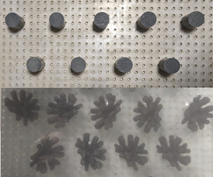
The coral canopy was modelled in two ways: first using cylindrical dowels (figure 2 $a$) and second using scaled coral replicates (figure 2
 $b$). The scaled coral replicates were chosen to match common coral head characteristics: randomly oriented branches and non-uniform mass distributed with height. Many coral species have a cylindrical base with branches concentrated near the top of the canopy (figure 1b–e). To get the coral replicates, scans of living Pocillopera meandrina heads (figure 1c) were scaled down and then 3-D-printed to a height of 5 cm (three-dimensional models were provided open source by The Hydrous, https://thehydro.us/3d-models). The coral replicas were mounted on cylindrical bases cut from the same cylinders used for the cylinder canopy. Both the cylinder and 3-D-printed corals were 7 cm tall, giving a submergence ratio of
  $h_c/h = 0.22$, where
  $h_c$ is the canopy height and
  $h$ is the water depth. The spacing was kept consistent between canopy cases with
  $s = 8\ {\rm cm}$,
  $d = 4\ {\rm cm}$ and
  $s/d = 2$ (figure 2c).

Figure 2. Canopy composition for (a) cylinders and (b) corals. Canopy element spacing and horizontal positions of velocity measurements are illustrated for (c) the cylinder canopy and (d) the coral canopy. Horizontal positions are evenly spaced ranging from directly behind the coral element (location 1) to in between two canopy elements (location 4).
Ideally, volume, frontal area and canopy height would all be identical between the coral and the cylinder canopy cases. However, given that the 3-D-printed corals were made from scans of real corals, it was only possible to match one of the three physical characteristics when scaling down the coral model. Between volume, frontal area and canopy height, past research suggests it is most critical to match  $h_c/h$ between the two canopy cases (McDonald, Koseff & Monismith Reference McDonald, Koseff and Monismith2006). This choice resulted in the cylinders having 20 % less volume and 33 %–47 % smaller frontal area than the corals (depending on coral orientation). Thus, this study focuses on differences caused by shape complexity. While it is not appropriate to directly compare free-stream velocity, in-canopy velocity or the ratio between the two for each of the two canopies, it is appropriate to compare the shape of profiles (i.e. location of peaks) and relative differences between profiles in different locations (i.e. discussion of defined wakes).
2.3. Velocity measurement system
A 2-component laser-Doppler Anemometer (LDA) was used to measure instantaneous streamwise  $u$ and vertical
  $w$ velocities. The entire LDA system was fixed to a platform with vertical and horizontal axis of motion. More details on the LDA system can be found in Mandel et al. (Reference Mandel, Rosenzweig, Chung, Ouellette and Koseff2017). Velocities were acquired at 14 heights above the bed:
  $z = [3.1, 3.9, 4.7, 5.5, 6.3, 8, 9.5, 11, 12.5, 15, 18, 21, 24, 27]\ {\rm cm}$, with
  $z = 0$ defined at the bed. We did not focus on capturing near-bed hydrodynamics in detail, as the primary goal of the experiment was to assess the overall flow similarities and differences behind and above the roughness elements. At each height, velocities were taken at four horizontal positions ranging from directly behind the canopy element to in between two canopy elements:
  $y/d = [0, 0.5, 1, 1.5]$ (figure 2c,d). Together, the instantaneous velocity profiles capture a representative range of the in-canopy and above-canopy dynamics. Measurement uncertainty comes from the following: vertical positioning of the LDA; the length of the time series; changes in water depth due to evaporation; the separation angle between the beams which affects estimates of
  $u$. The total measurement uncertainty is less than 5 % of the mean velocity.
2.4. Data processing
At each measurement location, a 10 minute time series of vertical and horizontal velocities was recorded at 200 Hz on average. The time series was despiked in a two-step process. First, all velocities above a non-physical threshold velocity were removed. The resulting time series was despiked using the phase-space method by Goring & Nikora (Reference Goring and Nikora2002) modified by Mori, Suzuki & Kakuno (Reference Mori, Suzuki and Kakuno2007). After despiking, the time series was then filtered down to a uniform 50 Hz using a Gaussian filter function with 50 % overlapping windows.
Velocities were then decomposed into mean and fluctuating components. Overbars signify time averaging and ‘ $'$’ signifies fluctuating components such that at any instant in time,
  $u= \bar {u} + u'$. Spectra were computed in four segments using a Hamming window with 50 % overlap.
3. Results
3.1. Mean velocity profiles
Streamwise flow for each canopy is shown in figure 3( $a$) for the cylinders and in figure 3(
 $b$) for the corals. Streamwise velocities are normalized by the free-stream velocity, which is
  $23\ {\rm cm}\ {\rm s}^{-1}$ for the cylinder case and
  $24\ {\rm cm}\ {\rm s}^{-1}$ for the coral case. To directly compare the two canopy cases, we plot the mean velocity profiles for the cylinders and corals together at location 1 (figure 3
 $c$) and location 4 (figure 3
 $d$). Figures 3(
 $c$) and 3(
 $d$) are normalized by the depth-averaged velocity,
  $q/h$, to keep the non-dimensionalization consistent between the two canopy cases. Here,
  $q$ is the volumetric flow rate per unit width (
 $q = Q/b$ where
  $b$ is the tank width) calculated by integrating the velocity profile from the bed to the free surface (assuming constant velocity over the top 5 cm in both cases).

Figure 3. Mean streamwise velocities for (a) cylinders and (b) corals at all locations normalized by the free-stream velocity  $u_{\infty}$, and comparison of mean streamwise velocities at (c) location 1 and (d) location 4 normalized by the depth-averaged streamwise velocity
  $q/h$.
Some of the more notable similarities and differences in the profiles are as follows. First, the cylinder profiles show a well-defined, narrow wake within the canopy ( $z/h < 0.22$) in the lee of the cylinders. This is illustrated by mean velocities less than 20 % of the free-stream velocity at locations 1 and 2 (inside the wake) compared with mean velocities greater than 40 % of the free-stream velocity at locations 3 and 4 (outside the wake). In contrast, the coral profiles show a broader wake. This observation is based on the less distinct difference between locations in the inner part of the wake (locations 1 and 2) and those on the outer portion of the wake (locations 3 and 4).
Second, the apparent wider influence of the corals (broader wake) seems to cause an overall slowdown of the flow within the canopy, with mean velocities at all locations less than 25 % of the free-stream velocity. In this experiment, the pump is set to maintain the same, constant flow rate for both experiments. Therefore, due to the increased resistance inside the coral canopy, there is a redistribution of velocity and consequently a greater fraction of the flow higher up in the water column (figure 3b,c). The differences in flow distribution between the in-canopy region and the free stream is due to a combination of the coral geometry and the larger coral frontal area, but it does not significantly impact overall drag due to a combination of factors that will be discussed in § 3.3.
Third, our results indicate more recirculation within the coral canopy. In-canopy velocities at location 1 are in negative (reverse flow), averaging to approximately 10 % of the free-stream velocity. Furthermore, the corals have a local minimum velocity at the height of the branches which is absent in the cylinder velocity profiles.
3.2. Turbulence characteristics
In addition to differing mean flows within the canopy, turbulence statistics also vary between the two cases. Specifically, the in-canopy Reynolds stresses exhibit different behaviours between cases (figure 4). At all locations, but specifically wake locations 1 and 2, the cylinders have a higher peak Reynolds stress at the top of the canopy. This peak is likely caused by flow separation and vortex shedding off the cylinder's sharp top edge. At location 2, the stress increase above the canopy may stem from shear from both the top and the side of the cylinder. In contrast, the coral profiles lack the sharp peak observed in the cylinder case but have on average higher Reynolds stresses above the canopy ( $z/h > 0.5$) at all locations, particularly locations 3 and 4. At location 4, higher in-canopy flow in the cylinder case leads to larger in-canopy stresses. The bootstrap uncertainties were at least an order of magnitude smaller than the Reynolds stress values and are too small to be discerned in figure 4.

Figure 4. Comparison between coral and cylinder Reynolds stress profiles for all horizontal locations.
Turbulent spectral density can also be used to evaluate similarities and differences between the two canopy cases. Coral and cylinder spectra are compared in wavenumber space to remove differences caused by varying free-stream velocities. Taylor's frozen turbulence hypothesis is used to convert between frequency space and wavenumber space. However, the theory breaks down within the canopy at locations 1 and 2, as the time-averaged velocity is too slow for the assumption  $\overline {u'^2} / \bar {u}^2 \ll 1$ to hold (Lin Reference Lin1953). Therefore, only spectra at locations 3 and 4 are plotted. Figure 5 shows that, within the canopy, the coral spectra have more energy at higher wavenumbers (smaller scales), and less energy at lower wavenumbers (larger scales).

Figure 5. Comparison between coral and cylinder wavenumber spectra at  $z/h = 0.15$ for horizontal location 3 and location 4, which is below the top of the canopy. The submergence ratio is
  $0.22$.
While in-canopy mean flows and turbulence statistics differ between cases, these differences become much less significant in the free stream (figure 6). Both canopies show similar rolloff behaviour and agree on all scales. To further examine how simplified corals affect the flow characteristics, we compared turbulent production profiles. In figure 7, production was calculated at each measurement height as
 \begin{equation} P ={-}\overline{u'w'} \frac{{\rm d}\bar{u}}{{\rm d}z} \end{equation}
(Pope Reference Pope2012). Here,  ${\rm d}\bar {u}/{\rm d}z$ was calculated by first fitting a cubic smoothing spline to the mean velocity profile by minimizing
  $f$ in the equation
 \begin{equation} p\sum_{j=1}^{n}|\bar{u}_j-f(z_j)|^2 + (1-p)\int \lambda(t)|D^2f(t)|^2\,{\rm d}t, \end{equation}
where  $n$ is the number of measurement heights,
  $D^2f(t)$ is the second derivative of
  $f$ and
  $\lambda = 1$ (de Boor Reference de Boor1980). The value of
  ${\rm d}\bar {u}/{\rm d}z$ was determined by evaluating the derivative of
  $f$ at each measurement height. Uncertainty associated with
  ${\rm d}\bar {u}/{\rm d}z$ was calculated by adjusting the fitting parameter
  $p$ in the range of
  $-4*10^{-7}$ to
  $+9*10^{-8}$. All values of
  $p$ within this range gave acceptable spline fits.

Figure 6. Comparison between coral and cylinder wavenumber spectra at  $z/h = 0.35$ for all horizontal locations. The submergence ratio is 0.22.

Figure 7. Comparison between coral and cylinder production profiles for all horizontal locations. Uncertainty comes from  ${\rm d}u/{\rm d}z$ estimates.
Above the canopy, there were no significant differences in production at any location. Within the canopy there were small, location-dependent variations. At locations 1 and 2, the cylinders had 45–90 % greater peak production (at  $z/h = 0.25$) than the corals due to the larger Reynolds stress from the cylinder's sharp top edge. However, these variations in production do not appear to be significant when considering the canopies’ integrated drag. If the corals created significantly more drag than the cylinders, the pressure at the beginning of the canopy would be higher for the corals than the cylinders. Although pressure at the beginning of the canopy was not measured directly, upstream water levels were monitored. We observed no difference in water depth either before the canopy or at the end of the canopy between the two cases. Thus, the identical water levels and similar friction velocities (discussed in § 3.3) strongly suggest overall drag effects were the same.
To examine the potential differences in mass transfer rates caused by using a simpler cylinder surrogate for the coral heads, we used turbulent dissipation as an indicator of the mixing that brings nutrients and gasses to coral surfaces. Dissipation was determined by fitting  $f^{-5/3}$ to the inertial subrange of the frequency spectra and then calculating
  $\epsilon$ as
 \begin{equation} \phi_{uu} = A \left(\frac{18}{55}\right) \epsilon^{2/3} \left(\frac{U}{2{\rm \pi}}\right)^{2/3} f^{{-}5/3}, \quad \phi_{ww} = \frac{4}{3} \phi_{uu}, \end{equation}
where  $A = 1.5$ (Nepf & Vivoni Reference Nepf and Vivoni2000). Dissipation was only evaluated above the canopy due to the high turbulence intensity relative to the mean streamwise velocity inside the canopy (Lumley Reference Lumley1965). Figure 8 shows the dissipation profiles for each location. The uncertainty in our measurements comes, in part, from disagreement between dissipation calculated from the streamwise velocity spectra and dissipation calculated using the vertical velocity spectra, even with the
  $4/3$ adjustment (3.3a,b). The maximum difference between dissipation calculated from
  $\phi _{uu}$ vs
  $\phi _{ww}$ occurred at the points closest to the top of the canopy. The frequency bounds of the inertial subrange
  $f^{-5/3}$ fit also contribute to uncertainty as there are multiple frequency bands where the linear regression of
  $f^{-5/3}$ is a good fit. Uncertainty associated with the
  $f^{-5/3}$ frequency band choice was quantified as the difference between
  $\epsilon$ calculated using the widest frequency range with a reasonable fit (6 hz) and
  $\epsilon$ calculated using the narrowest frequency range with a reasonable fit (3 hz). The uncertainty ranges associated with velocity spectrum choice and the uncertainty range frequency band choice were calculated as
 $$\begin{gather} \delta \epsilon_{d} = \left|\frac{\epsilon_{3\ {\rm Hz}, \phi_{uu}}+\epsilon_{6\ {\rm Hz}, \phi_{uu}}}{2}-\frac{\epsilon_{3\ {\rm Hz}, \phi_{ww}}+\epsilon_{6\ {\rm Hz}, \phi_{ww}}}{2}\right|, \end{gather}$$
 $$\begin{gather}\delta \epsilon_{f} = \left|\frac{\epsilon_{3\ {\rm Hz}, \phi_{uu}}+\epsilon_{3\ {\rm Hz}, \phi_{ww}}}{2}-\frac{\epsilon_{6\ {\rm Hz}, \phi_{uu}}+\epsilon_{6\ {\rm Hz}, \phi_{ww}}}{2}\right|, \end{gather}$$
 $$\begin{gather}\delta \epsilon = \sqrt{\delta \epsilon_{f}^2+\delta \epsilon_{d}^2}, \end{gather}$$
where  $\epsilon _{3\ {\rm Hz},\phi _{uu}}$ is the dissipation calculated by fitting
  $f^{-5/3}$ to a 3 Hz frequency band in
  $\phi _{uu}$,
  $\epsilon _{3\ {\rm H}z,\phi _{ww}}$ is the dissipation calculated by fitting
  $f^{-5/3}$ to a 3 Hz frequency band in
  $\phi _{ww}$,
  $\epsilon _{6\ {\rm Hz},\phi _{uu}}$ is the dissipation calculated by fitting
  $f^{-5/3}$ to a 6 Hz frequency band in
  $\phi _{uu}$ and
  $\epsilon _{6\ {\rm Hz},\phi _{ww}}$ is the dissipation calculated by fitting
  $f^{-5/3}$ to a 6 Hz frequency band in
  $\phi _{ww}$. Here,
  $\delta \epsilon _f$ is the uncertainty associated with frequency band choice,
  $\delta \epsilon _d$ is the uncertainty associated with differences in
  $\epsilon$ from using either
  $\phi _{uu}$ or
  $\phi _{ww}$ and
  $\delta \epsilon$ is the total uncertainty shown in figure 8.

Figure 8. Comparison between coral and cylinder dissipation for all horizontal locations. Uncertainty comes from differences in  $\epsilon$ due to which spectrum (
 $\phi _{uu}$ or
  $\phi _{ww}$)
  $\epsilon$ is calculated from and the sensitivity to inertial subrange frequency bounds.
At all locations, the dissipation peaks just above the canopy before decreasing with height. Although the coral canopy exhibits higher dissipation rates at all heights, the difference is within the uncertainty bounds. The close match of dissipation and production between the coral and cylinder cases, despite differences in frontal area, volume and mean velocity profiles within the canopy, indicates that precisely matching frontal area and volume has little impact on free-stream turbulence statistics.
Production and dissipation can be compared directly at each location to see if transport terms in the turbulent kinetic energy (TKE) equation significantly affect either canopy case (figure 9). As discussed above, dissipation was only plotted starting above the canopy, so further work is needed to examine transport terms within the canopy. There is good agreement in both canopy cases at heights where production and dissipation can be directly compared, with differences within uncertainty bounds, suggesting small TKE transport terms. The similarities between the corals and cylinders as shown in figures 8 and 7, therefore, strongly indicate that cylinders do an adequate job of capturing the overall structure of the boundary layer above a coral reef.

Figure 9. Comparison of spatially averaged production and dissipation profiles for each canopy type. Blue top row is the cylinder canopy case and red bottom row is the coral canopy case.
3.3. Estimating drag
The drag coefficient,  $C_D$, is necessary for determining the drag term in the momentum equation. Here,
  $C_D$ can be calculated as
 \begin{equation} C_D = u_*^2 / U_{ref}^2, \end{equation}
where  $u_*$ is the friction velocity and
  $U_{ref}$ is a reference velocity defined in the field as either velocity at 1 m above the bed or the depth-averaged velocity (e.g. Reidenbach et al. Reference Reidenbach, Monismith, Koseff, Yahel and Genin2006; Lentz et al. Reference Lentz, Davis, Churchill and DeCarlo2017). Given the highly resolved two-dimensional velocity profile, we are able to calculate
  $u_*$ using three separate method in order to evaluate the effect of canopy element simplification on drag estimates. All three methods described below are commonly used interchangeably in the field to calculated drag coefficients (Takeshita et al. Reference Takeshita, McGillis, Briggs, Carter, Donham, Martz, Price and Smith2016).
Log-fitting method: the friction velocity can be derived from fitting the velocity profile to the log law (Pope Reference Pope2012)
 \begin{equation} \bar{u}(z) = \frac{u_*}{\kappa} \ln\left(\frac{z-d}{z_0}\right), \end{equation}
where  $d$ is the displacement height and
  $\bar {u}(z)$ is the spatially averaged velocity profile. We begin log fitting at
  $2h_c$ to avoid accidentally fitting to the roughness sublayer which does not follow the log law (Brunet Reference Brunet2020). Because there are three fitting parameters (
 $u_*$,
  $z_0$ and
  $d$), values of
  $d$ were chosen to range from
  $z=0$ to
  $z=h_c$. All values of
  $d$ show excellent agreement with
  $R^2 > 0.93$ (figure 10a,c).

Figure 10. Log fits to spatially averaged velocity profile with various displacement heights ( $d$) and the resulting
  $u_*$ for (
 $a$) the cylinder canopy and (
 $b$) the coral canopy. The log law was fit to the filled circles only. Comparison of spatially averaged
  $u_*$ values calculated using the dissipation, covariance, and log-law methods for (
 $c$) the cylinder canopy and (
 $d$) the coral canopy. Vertical lines are log fit
  $u_*$ coloured by
  $d/h_c$.
Dissipation method: spectrally derived dissipation was used to calculate friction velocity as
 \begin{equation} u_* = (\epsilon \kappa z)^{1/3}, \end{equation}
where  $\kappa$ is the von Kármán constant and
  $z$ is the height above the bed. The dissipation-derived
  $u_*$ can only be calculated above the canopy (Lumley Reference Lumley1965).
Covariance method: the Reynolds stress at the bed can be related to the friction velocity (e.g. Lindhart et al. Reference Lindhart, Monismith, Khrizman, Mucciarone and Dunbar2021) as
 \begin{equation} u_* = \overline{|u'w'|_b}^{1/2}. \end{equation}
Above the bed, the Reynolds stress is expected to decrease linearly with height, reaching zero at the surface. Therefore, a depth correction must be added when using measurements higher up in the water column. Additionally, in the presence of large roughness elements, the maximum Reynolds stress occurs at approximately  $h_c$ instead of at the bed, so friction velocity is calculated as
 \begin{equation} u_* = \overline{|u'w'|_z}^{1/2}*\left( 1-\frac{z-h_c}{h-h_c}\right)^{{-}1/2}. \end{equation}
 For the dissipation and covariance methods, peak  $u_*$ occurs withing
  $1.5$ canopy heights, and then decreases with proximity to the surface. The values of
  $u_*$ for those two methods largely agree both across canopy cases and between methods. The agreement between canopy cases is likely due to opposing mechanisms. For the cylinder canopy, the sharp edge leads to a peak in shear stress which increases overall drag. For the coral canopy case, the steeper velocity gradient causes more instabilities, but the slower in-canopy flow results in a higher
  $U_{ref}$. Overall, this implies that individual shape complexity does not significantly impact overall drag (figure 10b,d).
However, across all values of  $d/h_c$,
  $u_*$ calculated using the log-fitting method is consistently higher in the coral canopy case than the cylinder case. It is also up to 3 times greater than
  $u_*$ calculated using dissipation and covariance methods, and very sensitive to displacement height choices (figure 10a,c). Typically,
  $u_*$ derived from log fits represents an integrated drag that incorporates changes in topography and patchiness, which has been noted in field studies (Rosman & Hench Reference Rosman and Hench2011). This experimental set-up represents a uniform canopy with no changes in topography or patchiness, suggesting that the corals are behaving (collectively) as a full canopy instead of as individual large roughness elements and a log layer does not exist. We caution the use of log fits to calculate drag coefficients when the submergence ration
  $h_c/h$ is of the order of 0.2 or greater, independent of canopy element complexity.
3.4. Parameter space considerations
This study is a detailed investigation of a relatively small parameter space. However, by carefully choosing the experimental parameters and using the results of related studies we can minimize the need for examining large parameter ranges. First, while varying the mean flow would produce a wider range of Reynolds numbers, once a flow is fully developed ( $Re > 10^4$), the Reynolds number has only a small effect on the turbulence dynamics and mixing (Dimotakis Reference Dimotakis2000). Second, cylinder size and spacing were chosen to match the spacing set in Lowe et al. (Reference Lowe, Koseff and Monismith2005a,Reference Lowe, Koseff, Monismith and Falterb). Lowe et al. (Reference Lowe, Koseff and Monismith2005a) showed that, as canopy spacing becomes denser (
 $S/d = 1$), the velocity inside the canopy decreases and the Reynolds stress increases. Both changes happen monotonically, suggesting a similarly monotonic change in the coral canopy as well. The differences in velocity and Reynolds stress are most significant within the canopy and only slightly affect the flow above the canopy, indicating that the above-canopy similarities between the corals and the cylinders will remain similar even with varied spacing.
Third, canopy flow depends on the submergence ratio  $h_c/h$ in that as submergence ratio increases, more flow is forced through the canopy (McDonald et al. Reference McDonald, Koseff and Monismith2006). In instances where canopy element simplification impacts results, we expect the impact to increase as submergence ratio increases. Finally, the coral canopy in this study consists of only one type of coral. Universally, corals have branches, smooth edges and bumpy surfaces (figure 1), so we chose a coral exhibiting all of these common features.
There are additional complexities not accounted for in this study. Since the experiment had unidirectional flume with uniformly distributed canopy elements, neither case captures the spatial and temporal complexities of living reefs, where coral coverage is typically heterogeneous and patchy. Furthermore, the 3-D-printed coral heads most closely resemble branching corals, and it has been shown that tabletop corals lead to a different ratio of in-canopy to free-stream flow (Pomeroy et al. Reference Pomeroy, Ghisalberti, Peterson and Farooji2023). Oscillatory flow also impacts both mass transfer (Lowe et al. Reference Lowe, Koseff, Monismith and Falter2005b) and larval dispersion (Reidenbach, Koseff & Koehl Reference Reidenbach, Koseff and Koehl2009; Reidenbach et al. Reference Reidenbach, Stocking, Szczyrba and Wendelken2021). Additional work needs to be done to apply these results to corals of varying geometries.
4. Conclusion
This work presents an experimental hydrodynamic comparison between a coral head canopy and a cylinder canopy allowing us to conclude the following. Cylinder canopies have defined, narrow wakes in the lee of the cylinders and higher stresses at the top of the canopy associated with the cylinder's sharp edges. In contrast, coral head canopies exhibit broader, more muted wakes. Additionally, the coral branches increase resistance within the canopy, consequently redistributing flow to higher up in the water column.
Despite these in-canopy differences and the introduction of additional shear at the top of the cylinder canopy, the turbulence statistics, mean velocities and friction velocities largely agree above the canopy. This indicates that the overall structure of the boundary layer above a coral reef canopy can be captured using simple geometric surrogates for coral heads. Consistent with Reidenbach et al. (Reference Reidenbach, Monismith, Koseff, Yahel and Genin2006), while skin drag is important for mass transfer rates and diffusion, it is form drag from larger-scale roughness that contributes most to overall canopy drag. Therefore, it may be practical to get estimates of drag from simplified geometries, especially when mean in-canopy and free-stream velocities are based on observed environmental conditions. The experimental results of this study suggest that exactly matching surface area and volume does not lead to significant changes in turbulence statistics or drag estimates. Instead, it is likely more imperative to replicate submergence ratio and canopy element spacing. However, because these results were obtained for a unidirectional flow only without waves, they should only be applied at high Keulegan–Carpenter numbers where drag, not inertia, dominates.
There are instances when it is likely more appropriate to use real coral heads instead of cylinders, specifically when the in-canopy dynamics is of primary importance. For example, small-scale topographical features play a larger role in mass transfer and diffusion rates which have been shown to be spatially dependent and peak at stagnation points (Chang et al. Reference Chang, Iaccarino, Ham, Elkins and Monismith2014). Additionally, studies show that larval transport and settlement is significantly affected by the local hydrodynamics (Crimaldi et al. Reference Crimaldi, Thompson, Rosman, Lowe and Koseff2002; Whitman & Reidenbach Reference Whitman and Reidenbach2012). Coral larvae favour tightly spaced roughness with less shear (Reidenbach et al. Reference Reidenbach, Stocking, Szczyrba and Wendelken2021), so the cylinder's sharp edge and the defined wake could lead to inaccurate model results. Previous work by McDonald et al. (Reference McDonald, Koseff and Monismith2006) suggests  $h_c/h$ plays a larger role in drag coefficient estimates in low Reynolds number flows, so using simplified roughness like cylinders may be less accurate in such cases.
Acknowledgements
We would like to thank the Stanford Oceans Department, and the Department of Civil and Environmental Engineering for their support of J.F.H., and the Bob and Norma Street Environmental Fluid Mechanics Laboratory, and Stanford's Office of the Vice Provost for Undergraduate Education Fellowship Program for their generous support of B.Z.K. We would also like to thank to C. Anderson and B. Sabala for their assistance with the experimental set-up and E. Boles for valuable discussions.
Declaration of interests
The authors report no conflict of interest.


