2.1. The Wilcox (Reference Wilcox2006) $k$–$\omega$ model

The widely used two-equation Wilcox (Reference Wilcox2006) $k$–$\omega$ turbulence model in its standard form with a buoyancy production term are expressed as

(2.1)\begin{gather} \frac{\partial \bar{\rho} k }{\partial t} + \bar{u}_j\frac{\partial \bar{\rho} k }{\partial x_j} = \bar{\rho} P_k - \bar{\rho} P_b - \bar{\rho} \beta^* k \omega + \frac{\partial }{\partial x_j} \left[ \left( \mu + \bar{\rho} \sigma^* \frac{k}{\omega} \right) \frac{\partial k}{\partial x_j} \right], \end{gather}

(2.2)\begin{gather} \frac{\partial \bar{\rho} \omega }{\partial t} + \bar{u}_j\frac{\partial \bar{\rho} \omega } {\partial x_j} ={-} \bar{\rho}P_{\omega} - \bar{\rho} \beta \omega^2 + \bar{\rho} \frac{\sigma_d}{\omega}\frac{\partial k}{\partial x_j}\frac{\partial \omega}{\partial x_j}+\frac{\partial}{\partial x_j}\left[ \left(\mu + \bar{\rho}\sigma \frac{k}{\omega} \right) \frac{\partial \omega} {\partial x_j} \right], \end{gather}

where $x_j$ are the Cartesian coordinates, $\mu$ is the dynamic fluid viscosity, $\nu =\mu /\bar {\rho }$ is the kinematic fluid viscosity, $\bar {\rho }$ is the density of the fluid and $t$ is the time. The specific Reynolds stress tensor is defined as

(2.3)\begin{equation} \tau_{ij} ={-} \overline{u_{i}' u_{j}'}, \end{equation}

where the overbar denotes Reynolds (ensemble) averaging and the prime superscript denotes turbulent fluctuations. In the $k$–$\omega$ model this is formulated via the Boussinesq approximation

(2.4)\begin{equation} \tau_{ij} = 2\nu_t S_{ij} - \frac{2}{3}k\delta_{ij}, \end{equation}

where $\nu _t$ is the eddy viscosity, $\delta _{ij}$ is the Kronecker delta and

(2.5)\begin{equation} S_{ij}=\frac{1}{2}\left(\frac{\partial \bar{u}_i}{\partial x_j} + \frac{\partial \bar{u}_j}{\partial x_i} \right) \end{equation}

is the mean strain rate tensor. In (2.1) the shear production term

(2.6)\begin{equation} P_k = \tau_{ij}\frac{\partial \bar{u}_i}{\partial x_j} \end{equation}

is formulated in the form of eddy viscosity (again via the Boussinesq approximation), i.e.

(2.7a,b)\begin{equation} P_k = p_0 \nu_t, \quad p_0 = 2S_{ij}S_{ij}. \end{equation}

The buoyancy production term is formulated as

(2.8a–c)\begin{equation} P_b= p_b \nu_t, \quad p_b= \alpha_b^{*} N^2, \quad N^2=\frac{g_i}{\rho_0}\frac{\partial \bar{\rho}}{\partial x_i}, \end{equation}

where $N^2=0.5 N_{ii}$ is half the trace of the Brunt–Väisälä frequency tensor expressed as

(2.9)\begin{equation} N_{ij}= \frac{1}{\rho_0} \left( g_i\frac{\partial \bar{\rho}}{\partial x_j} + g_j\frac{\partial \bar{\rho}}{\partial x_i}\right), \end{equation}

where $\rho _0$ is the constant reference density of the fluid and $g_j$ is the gravitational acceleration. The eddy viscosity is calculated by

(2.10)\begin{equation} \nu_t=\frac{k}{\tilde{\omega}}. \end{equation}

In the Wilcox (Reference Wilcox2006) $k$–$\omega$ model $\tilde {\omega }=\tilde {\tilde {\omega }}$, where

(2.11)\begin{equation} \tilde{\tilde{\omega}} = \max\left[\omega, \lambda_1\sqrt{\frac{p_0-p_b}{\beta^*}} \right], \end{equation}

which includes a so-called stress limiter via the second argument in the max function. Note that compared with the original Wilcox (Reference Wilcox2006) stress limiter, a buoyancy production $p_b$ is included for the two-phase (air and water) flow applications, in consistency with (2.1). Here, we have also introduced $\tilde {\tilde {\omega }}$ for later use in § 2.2. In (2.2) the production term for $\omega$ is expressed as

(2.12)\begin{equation} P_{\omega}= \alpha \frac{\omega}{k}\frac{\tilde{\omega}}{\tilde{\tilde{\omega}}}P_k = \alpha \frac{\omega}{\tilde{\tilde{\omega}}}p_0. \end{equation}

The closure coefficients are (Wilcox Reference Wilcox2006, Reference Wilcox2008)

(2.13)\begin{gather} \begin{aligned} \alpha & =0.52, \quad \beta^*=0.09, \quad \beta_0=0.0708, \quad \beta=\beta_0 f_{\beta}, \\ \sigma & =0.5,\quad \sigma^*=0.6,\quad \sigma_{d0}=0.125, \end{aligned} \end{gather}

(2.14)\begin{gather} \sigma_d= \begin{cases} 0, & \displaystyle \frac{\partial k}{\partial x_j}\frac{\partial \omega}{\partial x_j} \leq 0,\\ \sigma_{d0}, & \displaystyle \frac{\partial k}{\partial x_j}\frac{\partial \omega}{\partial x_j} > 0, \end{cases} \end{gather}

(2.15a–c)\begin{gather} f_{\beta}=\frac{1+85 \chi_{\omega}}{1+100 \chi_{\omega}},\quad \chi_{\omega}=\left\vert\frac{\varOmega_{ij}\varOmega_{jk}\hat{S}_{ki}}{(\beta^* \omega)^3} \right\vert, \quad \hat{S}_{ki}=S_{ki}-\frac{1}{2}\frac{\partial \bar{u}_m}{\partial x_m} \delta_{ki}. \end{gather}

In the present work, $\lambda _1=0.2$ and $\alpha _b^*=1.36$, following Larsen & Fuhrman (Reference Larsen and Fuhrman2018).

2.2. The stabilized Larsen & Fuhrman (Reference Larsen and Fuhrman2018) $k$–$\omega$ turbulence model

Previous CFD works on modelling progressive waves breaking on a sloped beach using two-equation models (e.g. the Wilcox (Reference Wilcox2006) $k$–$\omega$ model in § 2.1) have shown a persistent problem of over-production of turbulence in the potential flow region beneath surface waves; see, e.g. Lin & Liu (Reference Lin and Liu1998), Hsu, Sakakiyama & Liu (Reference Hsu, Sakakiyama and Liu2002), Brown et al. (Reference Brown, Greaves, Magar and Conley2016), Derakhti et al. (Reference Derakhti, Kirby, Shi and Ma2016), Devolder et al. (Reference Devolder, Troch and Rauwoens2018) and Qu et al. (Reference Qu, Liu and Ong2021). This over-production of turbulence has caused progressive waves to decay during long-time simulation even before reaching the breaking point. Larsen & Fuhrman (Reference Larsen and Fuhrman2018) have analysed several two-equation models and found that they are unconditionally unstable in the potential flow region beneath surface waves. They have then formally stabilized the two-equation models by reformulating the eddy viscosity. The stabilization approach involves a modification to $\tilde {\omega }$,

(2.16)\begin{equation} \tilde{\omega}=\max\left[ \tilde{\tilde{\omega}}, \lambda_2 \frac{\beta}{\beta^* \alpha } \frac{p_0}{p_{\varOmega}}\omega \right], \end{equation}

where

(2.17a,b)\begin{equation} p_{\varOmega}=2 \varOmega_{ij} \varOmega_{ij}, \quad \varOmega_{ij} =\frac{1}{2}\left(\frac{\partial \bar{u}_i}{\partial x_j} - \frac{\partial \bar{u}_j}{\partial x_i} \right) \end{equation}

and $\tilde {\tilde {\omega }}$ is as defined in (2.11). To limit the over-production of turbulence in the potential flow region, $\lambda _2=0.05$ was used in breaking wave simulations of Larsen & Fuhrman (Reference Larsen and Fuhrman2018), and is maintained in the present work. This model will be called the LF18 $k$–$\omega$ model in what follows. Note that with $\lambda _2=0$, then $\tilde {\omega }=\tilde {\tilde {\omega }}$ and this model essentially reverts back to the Wilcox (Reference Wilcox2006) $k$–$\omega$ model.

2.3. The Wilcox (Reference Wilcox2006) Reynolds stress–$\omega$ model

As found in the recent study of Li et al. (Reference Li, Larsen and Fuhrman2022), the Boussinesq approximation used in all two-equation models is the fundamental reason for their instability in the potential flow regions beneath non-breaking surface waves. In contrast to two-equation RANS models, Reynolds stress turbulence models (both $\omega$ and $\varepsilon$ types), e.g. the Launder–Reece–Rodistress–$\varepsilon$ model (Launder, Reece & Rodi Reference Launder, Reece and Rodi1975) or the stress–$\omega$ model (Wilcox Reference Wilcox2006), break free from the Boussinesq approximation. They were proved by Li et al. (Reference Li, Larsen and Fuhrman2022) to be neutrally stable for simulating non-breaking progressive wave trains, i.e. without having the problem of over-production of turbulence in the potential flow region beneath surface waves. Li et al. (Reference Li, Larsen and Fuhrman2022) then applied the Wilcox (Reference Wilcox2006) stress–$\omega$ model for simulating breaking waves on a sloped bed and achieved excellent accuracy, especially in the undertow velocity in the complicated inner surf zone, which even the best two-equation model in Larsen & Fuhrman (Reference Larsen and Fuhrman2018) (the LF18 $k$–$\omega$ model) failed to accurately simulate. The stress–$\omega$ model consists of six equations for the Reynolds stress components,

(2.18) $$\begin{align} \frac{ \partial \bar{\rho} \tau_{ij}}{\partial t} + \bar{u}_k \frac{\partial \bar{\rho} \tau_{ij}}{\partial x_k} &={-}\bar{\rho} P_{ij} + \frac{2}{3} \bar{\rho} \beta^* \omega k \delta_{ij} -\bar{\rho} \varPi_{ij}\nonumber\\ &\quad +\, \frac{\partial}{\partial x_k}\left[\bar{\rho} \left(\nu + \sigma^*\frac{k}{\omega}\right)\frac{\partial \tau_{ij}}{\partial x_k} \right] + \bar{\rho} \alpha_b^* \frac{k}{\omega} N_{ij} \end{align}$$

and one equation for the specific dissipation rate $\omega$, as given in (2.2). The shear production term for $\omega$ is

(2.19)\begin{equation} P_{\omega}=\alpha \frac{\omega}{k} P_k = \alpha \frac{\omega}{k} \tau_{ij}\frac{\partial \bar{u}_i}{\partial x_j}. \end{equation}

The pressure–strain correlation is

(2.20) $$\begin{align} \varPi_{ij} &= \beta^* C_1 \omega\left(\tau_{ij}+\frac{2}{3}k\delta_{ij}\right) -\hat{\alpha}\left(P_{ij}-\frac{2}{3}P\delta_{ij}\right) \nonumber\\ &\quad -\hat{\beta}\left(D_{ij}-\frac{2}{3}P\delta_{ij}\right) -\hat{\gamma}k\left(S_{ij}-\frac{1}{3}S_{kk}\delta_{ij}\right), \end{align}$$

where

(2.21)\begin{gather} P_{ij}=\tau_{im}\frac{\partial \bar{u}_j}{\partial x_m}+\tau_{jm} \frac{\partial \bar{u}_i}{\partial x_m}, \end{gather}

(2.22)\begin{gather} D_{ij}=\tau_{im}\frac{\partial \bar{u}_m}{\partial x_j}+\tau_{jm}\frac{\partial \bar{u}_m}{\partial x_i}, \end{gather}

(2.23)\begin{gather} P=\frac{1}{2}P_{kk}, \end{gather}

(2.24)\begin{gather} k ={-} \frac{1}{2} \tau_{kk}. \end{gather}

The last term in (2.18) is the buoyancy production term as derived in Li et al. (Reference Li, Larsen and Fuhrman2022), which is proportional to $N_{ij}$ from (2.9). The closure coefficients are (Wilcox Reference Wilcox2006)

(2.25)\begin{gather} \begin{gathered} C_1=1.8, \quad C_2=10/19, \quad \hat{\alpha}=(8+C_2)/11, \\ \hat{\beta}=(8C_2-2)/11, \quad \hat{\gamma}=(60C_2-4)/55,\quad \alpha=0.52, \\ \beta^*=0.09, \quad \beta_0=0.0708, \quad \beta=\beta_0 f_{\beta},\\ \sigma=0.5,\quad \sigma^*=0.6,\quad \sigma_{d0}=0.125,\end{gathered} \end{gather}

(2.26)\begin{gather} \sigma_d= \begin{cases} 0, & \displaystyle \frac{\partial k}{\partial x_j}\frac{\partial \omega}{\partial x_j} \leq 0,\\ \sigma_{d0}, & \displaystyle \frac{\partial k}{\partial x_j}\frac{\partial \omega}{\partial x_j} \geq 0, \end{cases} \end{gather}

(2.27a,b)\begin{gather} f_{\beta} =\frac{1+85 \chi_{\omega}}{1+100 \chi_{\omega}},\quad \chi_{\omega} =\left\vert\frac{\varOmega_{ij}\varOmega_{jk}\hat{S}_{ki}}{(\beta^* \omega)^3} \right\vert,\quad \hat{S}_{ki} =S_{ki}-\frac{1}{2}\frac{\partial \bar{u}_m}{\partial x_m} \delta_{ki} \end{gather}

and $\alpha _b^*=1.36$ as derived in Li et al. (Reference Li, Larsen and Fuhrman2022) (see their appendix A).

4.1. Influence of the turbulence closure models

The study of Qu et al. (Reference Qu, Liu and Ong2021) suggests that the choice of turbulence model will affect the breaking point relative to the pile. In this section we will therefore reinvestigate the influence of the turbulence model on the breaking point using a small Courant number (i.e. $Co=0.05$) and second-order accuracy of discretisation schemes. This again ensures good numerical accuracy in both free surface elevations and velocity kinematics, following Larsen et al. (Reference Larsen, Fuhrman and Roenby2019). In the next subsection we will discuss the effect of the Courant number on the breaking point. To investigate the influence of turbulence models on the breaking point in a cost-effective manner, we first remove the monopile at the end of the slope. Four 2-D simulations involving waves propagating up the $1\,{:}\,10$ slope are performed with (1) no turbulence model, (2) the Wilcox (Reference Wilcox2006) $k$–$\omega$ model, (3) the LF18 $k$–$\omega$ model and (4) the Wilcox (Reference Wilcox2006) stress–$\omega$ model.

Figure 2 presents the wave profiles and turbulence levels when the waves just begin to break at the location of the pile frontline (the pile location is added merely as a reference). The time instant is at $t/T=4.25$ when the waves have reached repeatable (periodic) status. It is interesting to see that using $Co=0.05$ and second-order schemes, the progressive waves break at the same location regardless of the turbulence model (indeed, even with no turbulence model). This contradicts Qu et al. (Reference Qu, Liu and Ong2021), but is in line with our own physical expectations: before wave breaking, there should be no significant turbulence production beneath the free surface, apart from the very thin boundary layer region near the bed (also evident in figure 2). Therefore, a laminar model (i.e. no turbulence model) should be able to accurately predict the wave profiles up to the onset of breaking. In the meantime, it should be expected that from wave shoaling on the slope to breaking on the cylinder front, the simulation with using an accurate (and stable, L18 $k$–$\omega$) turbulence model should behave very similar to that without a turbulence model. In short, the breaking point should not be altered by the choice of turbulence model if a stable turbulence model is properly applied and the simulation is converged. This is clearly demonstrated in figure 2.

Figure 2. Wave profiles and turbulence levels when the waves are breaking right at the location where the frontline of the monopile is located with (a) no turbulence model, (b) Wilcox (Reference Wilcox2006) $k$–$\omega$ model, (c) LF18 $k$–$\omega$ model, (d) Wilcox (Reference Wilcox2006) stress–$\omega$ model. The time instant is $t/T=4.25$ when the waves reached repeatable status. (Note that (d) is plotted with $k/(\omega \nu )$ as the stress–$\omega$ model does not utilize the eddy-viscosity assumption; this expression is comparable to $\nu _t/\nu$ for two-equation models.) (a) No turbulence model, $Co=0.05$. (b) Wilcox (Reference Wilcox2006) $k$–$\omega$ model, $Co=0.05$. (c) The LF18 $k$–$\omega$ model, $Co=0.05$. (d) Wilcox (Reference Wilcox2006) stress–$\omega$ model, $Co=0.05$.

Note that figure 2 is at an early time instant after waves reach a repeatable status. At this early time, the turbulence over-production with the Wilcox (Reference Wilcox2006) $k$–$\omega$ model (figure 2b) has not yet grown to a significant level. If we further run the simulations to over 50 wave periods, an obvious instability of the Wilcox (Reference Wilcox2006) $k$–$\omega$ model can be seen. Figure 3(a) further presents results at a time instant $t/T=50.25$, computed with the Wilcox (Reference Wilcox2006) $k$–$\omega$ model. It is shown that turbulence level has now largely increased in the pre-breaking region. This over-production of turbulence extracts energy from the propagating waves and decays the wave amplitude, thus causing the waves to gradually break later than in figure 2. As indicated by the dashed line in figure 3(a), the wave breaking point is behind the location of the pile frontline. This problem does not exist with the LF18 $k$–$\omega$ model (because of the stabilization), as shown in figure 3(b), where the turbulence at the pre-breaking region is kept small and the breaking point remains accurately on the pile frontline even after 50 wave periods. Similar results as in figure 3(b) have been achieved with the stress–$\omega$ model (because the model is neutrally stable), as well as with the no turbulence model; they are not shown here for the sake of brevity. A similar comparison and discussion can also be found in Larsen & Fuhrman (Reference Larsen and Fuhrman2018) and Li et al. (Reference Li, Larsen and Fuhrman2022).

Figure 3. Wave profiles and turbulence levels with (a) the Wilcox (Reference Wilcox2006) $k$–$\omega$ model and (b) the LF18 $k$–$\omega$ model at the time instant $t/T=50.25$. In (a) the vertical dashed line indicates the breaking point. (a) Wilcox (Reference Wilcox2006) $k$–$\omega$ model, $Co=0.05$. (b) The LF18 $k$–$\omega$ model, $Co=0.05$.

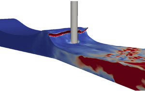
If we place the vertical pile in the tank, the same results can be reached, i.e. we find that the presence of the pile does not significantly alter the incipient breaking point. Figure 4 presents a screen shot for the 3-D simulation including the pile with waves initially breaking on the front surface of the pile. The simulation in figure 4 is performed with the stress–$\omega$ model at $t/T=8.25$ after waves reach a repeatable state. The fluid domain is coloured with the turbulent kinetic energy $k$. The red zone after breaking indicates high turbulent kinetic energy, while the blue zone prior to breaking indicates low turbulent kinetic energy. Similar scenarios have been observed using the LF18 $k$–$\omega$ model and other models, which are not shown here for brevity.

Figure 4. Screenshots of the 3-D simulation of waves breaking exactly on the vertical pile frontline at $t/T=8.25$, simulated with the Wilcox (Reference Wilcox2006) stress–$\omega$ model. (a) A 3-D view at the breaking instant. (b) Centre section ($y=0$) view at the breaking instant.

4.2. Effect of the Courant number

In this section we will further investigate the effect of the Courant number on the predicted breaking point. Figure 5 presents the 2-D breaking wave simulations (again, without the presence of the vertical pile) with the stress–$\omega$ model and with $Co$ ranging from 0.025 to 0.3. Figure 5(a,b) shows that with $Co=0.025$ and 0.05, the breaking point is on the frontline of the vertical pile, which is the same as that observed in the experiment (Irschik et al. Reference Irschik, Sparboom and Oumeraci2004) with the same wave condition and slope. This indicates that the breaking point is reasonably converged with $Co\leq 0.05$. However, as $Co$ is increased to 0.1 and larger, as shown in figure 5(c–e), the waves break earlier and earlier. Larsen et al. (Reference Larsen, Fuhrman and Roenby2019) demonstrated that for non-breaking wave simulations in OpenFOAM with the VOF method and PIMPLE algorithm (a combination of PISO – pressure implicit with splitting of operator – and SIMPLE – semi implicit method for pressure-linked equations), there is a tendency for surface elevations to increase and crest velocities to become severely overestimated, even over relatively short times. They found that a relatively small $Co$ is required to mitigate this problem. This implies that many past simulations may not have converged velocity kinematics, especially near the crest. The present study on breaking waves has demonstrated a similar phenomenon as the study on non-breaking progressive waves in Larsen et al. (Reference Larsen, Fuhrman and Roenby2019). It is hence found that a large $Co$ can alter the breaking point due to inaccurate flow kinematics, whereas maintaining $Co \leq 0.05$ can ensure reasonable convergence in the breaking position.

Figure 5. Computed wave profiles and turbulence levels at incipient breaking utilizing the Wilcox (Reference Wilcox2006) stress–$\omega$ model with various $Co$. Note that the case with $Co=0.05$ is a repeat of that shown in figure 2(d). Results are shown for (a) $Co=0.025$, (b) $Co=0.05$, (c) $Co=0.1$, (d) $Co=0.2$, (e) $Co=0.3$.

Interestingly, if a large $Co$ is used together with a two-equation turbulence model that is unstable in the potential flow region beneath waves (e.g. the standard $k$–$\omega$ model, the standard realizable $k$–$\varepsilon$ model, which has a tendency of turbulence over-production), the two errors could cancel each other, i.e. early breaking due to a large $Co$ may be delayed due to decreasing wave heights caused by the turbulence over-production and associated unphysical energy dissipation. In this way the waves may coincidentally break on the pile, but the waves would expectedly have both a polluted turbulence field and inaccurate velocity kinematics. This is what we believe occurred in the simulation of Qu et al. (Reference Qu, Liu and Ong2021): their simulation with $Co=0.5$ and the standard $k$–$\omega$ SST model showed that their waves broke right on the pile frontline after 40 wave periods, but their domain was clearly polluted by turbulence over-production prior to breaking (see their figure 11d).

5.1. Peak load cycle

Before comparing the forces, the time series of the surface elevation near the vertical pile are presented in figure 7 to validate the simulated waves. The surface elevation at $(x,y)=(-0.7\,\textrm {m},\ 1.9\,\textrm {m})$ was measured in Irschik et al. (Reference Irschik, Sparboom and Oumeraci2004) and presented in Choi et al. (Reference Choi, Lee and Gudmestad2015). Figure 7 shows the numerically predicted (i.e. with the Wilcox (Reference Wilcox2006) stress–$\omega$ model, the LF18 $k$–$\omega$ model and no turbulence model) and the experimentally measured surface elevation $\eta$. A good match is observed between all three numerical predictions and the experimental data. As no turbulence is produced before wave breaking, the results with the turbulence models are essentially the same as without. This further confirms that the choice of turbulence model should not affect the accuracy of wave-induced surface elevations before wave breaking.

Figure 7. Comparison of computed and measured (Irschik et al. Reference Irschik, Sparboom and Oumeraci2004) surface elevations at $(x,y)=(-0.7\,\textrm {m},\ 1.9\,\textrm {m})$. Here $t/T=0$ is defined at the seventh wave cycle when the simulation reaches a repeatable state (similarly on several forthcoming figures). In the legend, TM stands for turbulence model.

The peak force $F$ (i.e. the total horizontal force in the $x$ direction) induced by breaking waves on the vertical pile is presented in figure 8. Numerical predictions with the Wilcox (Reference Wilcox2006) stress–$\omega$ model, the LF18 $k$–$\omega$ model and no turbulence model are compared with the processed experimental data presented in Choi et al. (Reference Choi, Lee and Gudmestad2015). It is noted that the forces measured in the original experiments of Irschik et al. (Reference Irschik, Sparboom and Oumeraci2004) were recorded synchronously with a sampling rate of 200 Hz. In order to eliminate the amplified force component due to the structural vibration that was recorded in the experiment, Choi et al. (Reference Choi, Lee and Gudmestad2015) applied a low-pass filter of 20 Hz to cutoff the signal at the structural natural frequency and used the empirical mode decomposition (EMD, by taking the mean of the upper and lower signal envelope) to separate the net breaking wave force from the measured data. Figure 8 compares the processed (with both the low-pass filter and EMD) experimental data presented by Choi et al. (Reference Choi, Lee and Gudmestad2015) with the present numerical results. In figure 8, $t_D \approx 0.02 T$ is the duration of the sharp peak (or slamming force). It is seen that all three numerical simulations can predict the slamming duration reasonably in line with the measurement. However, it is noted that the numerical predictions of the peak force are generally higher than the processed experimental data. This might be due to the EMD applied in Choi et al. (Reference Choi, Lee and Gudmestad2015) to process the experimental data that significantly reduced the peak value. Figure 9(a) alternatively compares the computed force results from all three models with the low-pass filtered experimental force from Choi et al. (Reference Choi, Lee and Gudmestad2015), without EMD. It can therefore be seen that the peak experimental force (approximately $1.8\times 10^4$ N) matches quite well with those computed (e.g. $1.6\times 10^4$ N, as predicted with the stress–$\omega$ model). Both of these values are above the experimental peak (1.2 $\times 10^4$ N) when both low-pass filtering and EMD are applied. In figure 9(b) we additionally compare the numerical results from the stress–$\omega$ model (black line) with both the unfiltered (raw) force signal (digitized from Choi et al. (Reference Choi, Lee and Gudmestad2015), green dotted line) and the same signal after application of low-pass filtering and EMD (red dotted line, as in figure 8). It can be seen in figure 9(b) that the peak force computed with the stress–$\omega$ model is in between the raw (unfiltered) and the processed (low-pass filter and EMD) peaks. Based on the comparisons in figure 9, and the differences in the model (fixed monopile) versus that used in the experiment, the computed peak force appears reasonable. It is likewise clearly seen from figure 9 that during the rise leading up to the peak ($t/T<0.25$), and also during the SLC ($t/T> 0.4$), neither the low-pass filter or EMD affect the force amplitude significantly. Therefore, in the discussion of SLC that follows, we adopt the processed (i.e. both low-pass filtered and EMD) experimental force signal for comparison. Note that this processed experimental data are available for a longer time duration during the SLC, as presented in Jose et al. (Reference Jose, Choi, Giljarhus and Gudmestad2017).

Figure 8. Instantaneous peak force from the present numerical predictions and the measured data processed in Choi et al. (Reference Choi, Lee and Gudmestad2015) with a low-pass filter and empirical mode decomposition (EMD).

Figure 9. Comparison of forces among selected numerical predictions and (a) the filtered experimental force without EMD and (b) the raw experimental force and after application of both filter and EMD. All experimental data are from Choi et al. (Reference Choi, Lee and Gudmestad2015).

Another common feature that can be noted for all three numerical results is that they predict an almost identical rise leading up to the peak force and more or less the same peak value. This is again because the peak force is measured right at the onset of wave breaking. From pre-breaking up to the breaking onset, we expect that even with no turbulence model, the peak force should be accurately predicted, as argued above. Our numerical results are in line with this expectation. This draws an unsurprising, but apparently new, conclusion, that a proper application of turbulence models should not alter the numerical prediction of the peak force when waves incipiently break right on the frontline of a vertical cylinder. Indeed, no previous studies have shown this result (likely due to the large Courant number and/or unstable turbulence models utilized). However, it is emphasized that this conclusion is only valid for cases where waves initially break right on the structure. If a wave breaks prior to reaching the structure, a turbulence model must be used to predict the wave force on the structure, as this becomes a post-breaking problem and breaking-induced turbulence will have been produced. It is also worthwhile to mention that to reach convergence, $Co=0.05$ is applicable for wave simulations using the VOF method, ensuring good accuracy in the velocity field beneath the surface. This may not be a universal criterion for all kinds of RANS-based simulations, however.

5.2. Secondary load cycle

Following the peak force, a SLC occurs for the present case. The predicted SLC is compared with the experimental data in figure 10. It is seen that the numerical predictions in each subfigure reasonably capture the duration of the SLC, defined according to Chaplin et al. (Reference Chaplin, Rainey and Yemm1997) as the horizontal time span from points A to B in each subfigure, corresponding to approximately 11 % of the wave period. The amplitude of the SLC is defined as the vertical force difference between points C and D. The numerical predictions of the so-called SLC ratio, i.e.  the SLC load divided by the numerical peak force, are around 3 % for all the numerical predictions. Previous experimental studies, e.g. Grue et al. (Reference Grue, Bjørshol and Strand1993), have reported amplitudes of the SLC up to 11 % of the peak force. The present numerical predictions are below this value.

Figure 10. Secondary load cycle by numerical predictions and the experimental measurement.

Although the numerical predictions with all three models seem to be able to reasonably capture the SLC load and duration, figure 10(b) shows an obvious magnitude difference of the force during the SLC between the LF18 $k$–$\omega$ prediction and the experimental data (almost double in the minimum force). The no turbulence model prediction of the force magnitude during the SLC in figure 10(c) is somewhere in between the numerical results in figure 10(a,b). Figure 10(a) presents a good match between the stress–$\omega$ model prediction and the measurement of the force magnitude during the SLC.

To provide an in-depth look of each simulation on the SLC, turbulence characteristics around the pile are investigated as follows. We have concluded earlier that the accurate peak force prediction is essentially independent of the turbulence model utilized. However, as the SLC is generated after wave breaking and is associated with the flow around the cylindrical body, turbulence models are expected to have a more significant effect on the SLC predictions. Figure 11 shows the vorticity field at $z=-D/2$ at $t/T=0.49$, when the SLC reaches its local peak (see figure 10). It is seen that with the stress–$\omega$ model in figure 11(a), a strong vortex pair is formed in the lee-wake of the pile. Vortex shedding does not occur for this condition, as the Keulegan–Carpenter number ($KC=U_m T/D$, where $U_m$ is the amplitude of the flow velocity oscillation) is small with $KC\approx 6$ at $z=-D/2$, such that the flow changes direction prior to vortices being shed. A detailed discussion of $KC$ and the vortex shedding can be found in Li et al. (Reference Li, Ong, Fuhrman and Larsen2020). The prediction with the LF18 $k$–$\omega$ model in figure 11(b) shows a weaker vortex pair attached to the pile. However, when predicting with no turbulence model, as shown in figure 11(c), the flow separation and vortex field are completely different. We expect this result is wrong as it would be necessary to refine the computational mesh and the time step to a DNS simulation level to ensure the turbulence is resolved, which is not practical for the present 3-D wave–structure interaction case. The simulation with no turbulence model in the present study utilizes the same mesh as with turbulence models on. Therefore, in the turbulent region, the turbulence is not solved in a physically correct manner. Thereby, the simulation with no turbulence model is dropped in the following analysis. When comparing figures 11(a) and 11(b), a stronger vorticity field is predicted with the stress–$\omega$ model, which in turn causes larger magnitude negative pressure on the lee side during the flow reversal. This generates a stronger suction force on the lee side and raises the total horizontal force up in figure 10(a), which matches much better with the measurement.

Figure 11. Vorticity field with (a) the Wilcox (Reference Wilcox2006) stress–$\omega$ model, (b) the LF18 $k$–$\omega$ model and (c) no turbulence model at $z=-D/2$ and time instant of $t/T$=0.49, i.e. the local peak of the SLC.

Figure 12 further presents the 3-D coherent vortical structures identified by the $Q$ criterion simulated with the stress–$\omega$ model and the LF18 $k$–$\omega$ model. The $Q$ criterion (Dubief & Delcayre Reference Dubief and Delcayre2000) is the second invariant of the velocity gradient tensor, which is defined as

(5.1)\begin{equation} Q=\frac{1}{2}\left( S_{ij}^2-\varOmega_{ij}^2 \right). \end{equation}

Instantaneous isosurfaces corresponding to $Q=200\,\textrm {s}^{-2}$ in the water phase are shown in figure 12 at two time instants, i.e. when the waves are just breaking on the pile front ($t/T= 0.28$) and when the SLC reaches its local maximum ($t/T = 0.49$). The isosurfaces shown in figure 12(a) with the Wilcox (Reference Wilcox2006) stress–$\omega$ model and 12(c) with the LF18 $k$–$\omega$ model are similar at the wave breaking instant. The slight temporal difference is due to minor model differences. However, comparing figures 12(b) and 12(d) at the SLC local peak, obviously different structures are observed in the lee wake of the pile. Figure 12(b) with the stress–$\omega$ model predicts the pair of lee-wake vortices that were also shown in the DNS study of Jang et al. (Reference Jang, Ozdemir, Liang and Tyagi2021) at $KC=6$ (though in that study waves were simplified to oscillatory flows without considering the free surface). It is also noted that the formed vortex pair are tilting toward the bottom because of the boundary layer effect near the bottom wall. However, the isosurfaces simulated with the LF18 $k$–$\omega$ model do not demonstrate this feature; the lee-wake vortices were not clearly formed.

Figure 12. Instantaneous $Q=200\,\textrm {s}^{-2}$ isocontours in the vicinity of the vertical pile at the wave breaking instant and the local peak of SLC. Results are shown for (a) $t/T=0.28$, Wilcox (Reference Wilcox2006) stress–$\omega$ model; (b) $t/T=0.49$, Wilcox (Reference Wilcox2006) stress–$\omega$ model; (c) $t/T=0.28$, LF18 $k$–$\omega$ model; (d) $t/T=0.49$, LF18 $k$–$\omega$ model.

The differences in the vorticity field and the vortex formation are strongly linked to the flow separation. Figure 13 presents the horizontal velocity field $\bar {u}$ and compares the separation points for the Wilcox (Reference Wilcox2006) stress–$\omega$ model and the LF18 $k$–$\omega$ model. The separation point is defined as the point where the wall shear stress becomes zero, i.e. $(\partial u/\partial n)|_{wall}=0$. In each subfigure the red dots indicate the separation points from the stress–$\omega$ model and green squares from the LF18 $k$–$\omega$ model. It is observed that the flow separates further downstream with the LF18 $k$–$\omega$ model. This indicates that the simulated flow is more turbulent with the LF18 $k$–$\omega$ model than with the Wilcox (Reference Wilcox2006) stress–$\omega$ model. A simple explanation for this is that the more turbulent boundary layer has greater mixing of momentum with the outer flow, thus delaying the separation. A closer look at the turbulence field near the boundary of the pile is presented in figure 14 at $z=-D/2$. It is seen that as flow travels from the upstream point along the pile surface, the turbulent kinetic energy $k$ around the pile is indeed higher when predicted with the LF18 $k$–$\omega$ model than with the stress–$\omega$ model. Well-known shortcomings associated with the two-equation model, e.g. that the turbulence field near the curved surface is not accurately predicted, lead to later separation points and further underestimated vortex strength on the lee side.

Figure 13. Horizontal velocity field with (a) the Wilcox (Reference Wilcox2006) stress–$\omega$ model and (b) the LF18 $k$–$\omega$ model at $z=-D/2$ and the time instant of $t/T$=0.49, i.e. the peak of the SLC. In each subfigure red dots indicate the separation points from the Wilcox (Reference Wilcox2006) stress–$\omega$ model and green squares from the LF18 $k$–$\omega$ model. The red dashed lines in (b) indicate the locations of separation points projected from (a).

Figure 14. Turbulent kinetic energy around the pile at $z=-D/2$ and the time instant of $t/T=0.49$, simulated with (a) the Wilcox (Reference Wilcox2006) stress–$\omega$ model and (b) the LF18 $k$–$\omega$ model.

It can be seen from the discussion above that as the SLC is generated after wave breaking, it is closely associated with the flow around the cylindrical body. Thus, accurate turbulence modelling has a significant effect on the SLC predictions. Although some existing studies have claimed that the SLC is not necessarily linked to the flow separation (e.g. Grue et al. Reference Grue, Bjørshol and Strand1993; Ghadirian & Bredmose Reference Ghadirian and Bredmose2020), the flow separation point does affect the SLC amplitude when it occurs. Therefore, accurate turbulence modelling is seemingly required to predict the SLC. The present study demonstrates the advantage of using the stress–$\omega$ model, which breaks free from the traditional Boussinesq approximation for this purpose. Therefore, this model is able to predict both the peak and SLCs accurately.