


1. Introduction and background
Free-stream turbulence (FST) induced transition is one of the many routes to turbulence that can take place in a boundary layer. Due to its relevance in engineering applications, there has been produced abundant work in the topic. From all these investigations, we have a general good understanding of the process and steps involved in this scenario. This route to transition is initiated with the receptivity of free-stream disturbances which can be of linear or nonlinear nature (Brandt et al. Reference Brandt, Henningson and Ponziani2002), followed by the formation and amplification of streaks due to the lift-up effect (Landahl Reference Landahl1980). The emergence of secondary instabilities causes the final streak breakdown, resulting in the nucleation of turbulent spots (Schlatter et al. Reference Schlatter, Brandt, de Lange and Henningson2008) and the subsequent fully turbulent boundary layer. For the interested reader, a more detailed description of the whole process can be found, for instance, in Matsubara & Alfredsson (Reference Matsubara and Alfredsson2001); Brandt et al. (Reference Brandt, Schlatter and Henningson2004); Zaki (Reference Zaki2013).
In spite of the numerous experimental and numerical available evidence at our disposal, there are still some details that remain elusive. This is generally attributed to the dependence not only on the specific boundary conditions for each case dictating the stationary base flow, but also on the characteristics of the imposed FST. The latter is commonly defined from its turbulence intensity
 $Tu$
and an integral length scale
$Tu$
and an integral length scale
 $L_{11}$
, which is obtained from two-point correlation measurements and that determines how energy is distributed along the broadband FST spectrum. From an application perspective, probably the most interesting quantity is the streamwise position where transition to turbulence will take place under certain conditions. While the effect of
$L_{11}$
, which is obtained from two-point correlation measurements and that determines how energy is distributed along the broadband FST spectrum. From an application perspective, probably the most interesting quantity is the streamwise position where transition to turbulence will take place under certain conditions. While the effect of
 $Tu$
is well understood, the same is not true for
$Tu$
is well understood, the same is not true for
 $L_{11}$
. Notably, Fransson & Shahinfar (Reference Fransson and Shahinfar2020) showed in the same experimental campaign that depending on the
$L_{11}$
. Notably, Fransson & Shahinfar (Reference Fransson and Shahinfar2020) showed in the same experimental campaign that depending on the
 $Tu$
level, decreasing
$Tu$
level, decreasing
 $L_{11}$
can promote or delay transition, which goes against the general trend observed in previous investigations where only delay was observed (see, for instance, Brandt et al. Reference Brandt, Schlatter and Henningson2004; Jonáš et al. Reference Jonáš, Mazur and Uruba2000). This result motivated the work by Durović et al. (Reference Durović, Hanifi, Schlatter, Sasaki and Henningson2024), where an advance in transition was observed in a numerical simulation.
$L_{11}$
can promote or delay transition, which goes against the general trend observed in previous investigations where only delay was observed (see, for instance, Brandt et al. Reference Brandt, Schlatter and Henningson2004; Jonáš et al. Reference Jonáš, Mazur and Uruba2000). This result motivated the work by Durović et al. (Reference Durović, Hanifi, Schlatter, Sasaki and Henningson2024), where an advance in transition was observed in a numerical simulation.
The results for a zero pressure gradient (ZPG) flat plate in Fransson & Shahinfar (Reference Fransson and Shahinfar2020) led to the hypothesis that an optimal ratio between
 $L_{11}$
and the boundary-layer thickness at transition position
$L_{11}$
and the boundary-layer thickness at transition position
 $\delta _{tr}=\sqrt {\nu x_{tr}/U_\infty }$
must exist, with
$\delta _{tr}=\sqrt {\nu x_{tr}/U_\infty }$
must exist, with
 $\nu$
the kinematic viscosity and
$\nu$
the kinematic viscosity and
 $U_\infty$
the free-stream velocity. This ratio should be optimal in the sense that transition happens closest to the leading edge for a fixed turbulence intensity. One drawback on the use of this parameter is that it includes the streamwise position
$U_\infty$
the free-stream velocity. This ratio should be optimal in the sense that transition happens closest to the leading edge for a fixed turbulence intensity. One drawback on the use of this parameter is that it includes the streamwise position
 $x_{tr}$
where transition takes place, which is actually the quantity we are searching for. Nevertheless, this problem can be seen as finding the optimal
$x_{tr}$
where transition takes place, which is actually the quantity we are searching for. Nevertheless, this problem can be seen as finding the optimal
 $L_{11}$
such that unstable/breaking streaks arise closest to the leading edge.
$L_{11}$
such that unstable/breaking streaks arise closest to the leading edge.
The stability of streaks, and the resultant appearance of secondary instabilities, has been generally associated with their amplitude (Andersson et al. Reference Andersson, Brandt, Bottaro and Henningson2001), where optimal disturbance theory (Andersson et al. Reference Andersson, Berggren and Henningson1999; Luchini Reference Luchini2000) gives us the most likely waves due to their maximum amplification. However, it has also been proposed that the amplitude might not be the only relevant parameter to discriminate between stable and unstable streaks. For instance, the discrimination based on a neural network by Hack & Zaki (Reference Hack and Zaki2016) suggests that other quantities such as the wall-normal velocity, streamwise momentum and the spanwise shear can be valuable parameters to take into account for the identification of breaking streaks.
One stage of FST induced transition that is not always easy to account for is receptivity, setting the scale and initial amplitude of the disturbances inside the boundary layer. In this regard, a linear and a nonlinear mechanism have been proposed (Brandt et al. Reference Brandt, Henningson and Ponziani2002). The linear mechanism is characterised by the direct penetration of free-stream vortices into the boundary layer, taking place close to the leading edge. On the other hand, the nonlinear mechanism can occur along the whole boundary layer through triad interactions. In the work by Durović et al. (Reference Durović, Hanifi, Schlatter, Sasaki and Henningson2024), this latter mechanism was proposed as being responsible for turbulent spot inception. The reason being that the observed breaking streaks had a relative short spanwise wavelength, and those scales were not energetic close to the leading edge. This energy transfer can be explained by the preferred energy propagation towards higher spanwise wavenumbers (short wavelengths) through the
 $\beta$
-cascade proposed by Henningson et al. (Reference Henningson, Lundbladh and Johansson1993).
$\beta$
-cascade proposed by Henningson et al. (Reference Henningson, Lundbladh and Johansson1993).
The purpose of the present work is to document different simulations of FST induced transition performed within our group where we have observed that secondary instabilities, and therefore their hosting streaks, have a similar spanwise extension in their local boundary-layer scaling. Here, we also include some examples found in the literature. Further evidence that breaking streaks generally reach a certain aspect ratio condition can also be found in the work by Hack & Zaki (Reference Hack and Zaki2016), where they showed that for different pressure gradients, the shapes of breaking streaks were almost identical when scaled by the momentum thickness at transition position. By analysing the perturbations’ optimal growth, we see that the width of the breaking streaks are in the range of those reaching maximum amplification.
The remainder of this paper is structured as follows. In § 2 we present the framework for stability analysis. Section 3 includes the list of cases with their corresponding unstable modes. And finally, in § 4 we expand on some concluding remarks.
2. Stability analysis
The stability of the flow fields is studied in the local framework on planes normal to the streamwise direction. These planes are taken directly from the direct numerical simulation (DNS) solutions upstream and at previous time steps of a turbulent spot nucleation. In this context, we decompose the velocity and pressure field as
 \begin{equation} \mathbf {Q} (t,x,y,z) = \mathbf {Q}_0 (y,z;t,x) + \varepsilon \mathbf {q}(t,x,y,z), \end{equation}
with
 $\mathbf {x}=(x,y,z)^{\mathsf {T}}$
the streamwise, wall-normal and spanwise coordinates,
$\mathbf {x}=(x,y,z)^{\mathsf {T}}$
the streamwise, wall-normal and spanwise coordinates,
 $\mathbf {Q}_0=(U,V,W,P)^T$
the DNS solution for the velocity vector
$\mathbf {Q}_0=(U,V,W,P)^T$
the DNS solution for the velocity vector
 $(U,V,W)^T$
along the corresponding coordinates and the pressure
$(U,V,W)^T$
along the corresponding coordinates and the pressure
 $P$
, and
$P$
, and
 $\varepsilon$
the perturbation amplitude with corresponding shape
$\varepsilon$
the perturbation amplitude with corresponding shape
 $\mathbf {q}=(u,v,w,p)^{\mathsf {T}}$
. For the perturbation function, we assume a normal mode in time and along the streamwise direction
$\mathbf {q}=(u,v,w,p)^{\mathsf {T}}$
. For the perturbation function, we assume a normal mode in time and along the streamwise direction
 $\mathbf {q}=\hat {\mathbf {q}}(y,z)\exp (-i(\alpha x - \omega t))$
, with
$\mathbf {q}=\hat {\mathbf {q}}(y,z)\exp (-i(\alpha x - \omega t))$
, with
 $\alpha$
the streamwise wavenumber and
$\alpha$
the streamwise wavenumber and
 $\omega$
a complex value whose real and imaginary parts represent the angular frequency and temporal growth rate, respectively. The use of a local temporal framework for the stability analysis is justified by the time-scale separation between the low-frequency streaks and their high-frequency secondary instabilities. Examples of similar procedures can be found, for instance, in Hack & Zaki (Reference Hack and Zaki2014); Faúndez Alarcón et al. (Reference Alarcón, José, Cavalieri, Hanifi and Henningson2024a
).
$\omega$
a complex value whose real and imaginary parts represent the angular frequency and temporal growth rate, respectively. The use of a local temporal framework for the stability analysis is justified by the time-scale separation between the low-frequency streaks and their high-frequency secondary instabilities. Examples of similar procedures can be found, for instance, in Hack & Zaki (Reference Hack and Zaki2014); Faúndez Alarcón et al. (Reference Alarcón, José, Cavalieri, Hanifi and Henningson2024a
).
By substituting (2.1) in the Navier–Stokes equations and neglecting high-order terms we obtain the system
 \begin{align} \left ( \mathcal{C}- \varDelta \right ) \hat {u} + \left ( \mathcal{D}_{y} U\right ) \hat {v} + \left (\mathcal{D}_{z} U\right ) \hat {w} + i\alpha \hat {p} &= i\omega \hat {u}, \end{align}
 \begin{align} \left ( \mathcal{C}- \varDelta + \mathcal{D}_{y}V \right ) \hat {v} + \left (\mathcal{D}_{z} V \right ) \hat {w} + \mathcal{D}_{y} \hat {p} &= i\omega \hat {v}, \end{align}
 \begin{align} \left (\mathcal{D}_{y} W \right ) \hat {v}+\left ( \mathcal{C}- \varDelta + \mathcal{D}_{z}W \right ) \hat {w}+ \mathcal{D}_{z} \hat {p} &= i\omega \hat {w}, \end{align}
 \begin{align} i \alpha \hat {u} + \mathcal{D}_{y} \hat {v} + \mathcal{D}_{z} \hat {w} &= 0 , \end{align}
where
 $\mathcal{C}=U i\alpha + V \mathcal{D}_y + W\mathcal{D}_z$
,
$\mathcal{C}=U i\alpha + V \mathcal{D}_y + W\mathcal{D}_z$
,
 $\varDelta =1/{Re} (-\alpha ^2+\mathcal{D}_y^2 + \mathcal{D}_z^2 )$
,
$\varDelta =1/{Re} (-\alpha ^2+\mathcal{D}_y^2 + \mathcal{D}_z^2 )$
,
 $\mathcal{D}_y=\partial /\partial y$
and
$\mathcal{D}_y=\partial /\partial y$
and
 $\mathcal{D}_z=\partial /\partial z$
, where
$\mathcal{D}_z=\partial /\partial z$
, where
 $Rey$
is the Reynolds number. The discrete differential operators are built with a 4th-order finite difference scheme, while non-slip is imposed at the wall, periodicity along the span, and zero velocity in the far field. The generalised eigenvalue problem (2.2) is solved with a shift-and-invert Arnoldi algorithm.
$Rey$
is the Reynolds number. The discrete differential operators are built with a 4th-order finite difference scheme, while non-slip is imposed at the wall, periodicity along the span, and zero velocity in the far field. The generalised eigenvalue problem (2.2) is solved with a shift-and-invert Arnoldi algorithm.
3. Results
We present a summary of the analysed cases in table 1. The simulations consider different geometries, with and without leading edge, solvers, FST conditions and transition positions. However, they all share the same typical features of bypass transition from the inception to streak breakdown. The FST conditions,
 $Tu$
and
$Tu$
and
 $L_{11}$
, correspond to those reported in the respective work at the leading edge/inflow. For better comparison, they have been made non-dimensional by the momentum thickness
$L_{11}$
, correspond to those reported in the respective work at the leading edge/inflow. For better comparison, they have been made non-dimensional by the momentum thickness
 $\theta _0$
at
$\theta _0$
at
 ${Re}_\theta =116$
, which only coincides with the inlet condition in Sasaki et al. (Reference Sasaki, Morra, Cavalieri, Hanifi and Henningson2019). Evidently, this means that the reported values in table 1 for
${Re}_\theta =116$
, which only coincides with the inlet condition in Sasaki et al. (Reference Sasaki, Morra, Cavalieri, Hanifi and Henningson2019). Evidently, this means that the reported values in table 1 for
 $Tu$
and
$Tu$
and
 $L_{11}$
do not necessarily have those values at
$L_{11}$
do not necessarily have those values at
 ${Re}_\theta =116$
due to turbulence decay. The columns corresponding to
${Re}_\theta =116$
due to turbulence decay. The columns corresponding to
 ${Re}_{x_1}$
and
${Re}_{x_1}$
and
 ${Re}_{\theta _1}$
in table 1 represent the position where the stability analysis was performed for the corresponding simulation. Besides of the differences between cases, it is worth emphasising that these planes were taken upstream and at previous time steps from turbulent spot nucleations. The nucleation events were identified from flow inspection and laminar–turbulent discrimination of the fields, following the procedure described in Faúndez Alarcón et al. (Reference Alarcón, José, Cavalieri, Hanifi and Henningson2024a
).
${Re}_{\theta _1}$
in table 1 represent the position where the stability analysis was performed for the corresponding simulation. Besides of the differences between cases, it is worth emphasising that these planes were taken upstream and at previous time steps from turbulent spot nucleations. The nucleation events were identified from flow inspection and laminar–turbulent discrimination of the fields, following the procedure described in Faúndez Alarcón et al. (Reference Alarcón, José, Cavalieri, Hanifi and Henningson2024a
).
Table 1. List of the study cases. The LE column indicates if the simulation includes the leading edge. Here
 $Tu$
and
$Tu$
and
 $L_{11}$
represent the free-stream turbulence characteristics;
$L_{11}$
represent the free-stream turbulence characteristics;
 ${Re}_{x_1}$
and
${Re}_{x_1}$
and
 ${Re}_{\theta _1}$
correspond to the position where the stability calculations were performed.
${Re}_{\theta _1}$
correspond to the position where the stability calculations were performed.


Figure 1. Momentum thickness
 $\theta$
of the three base flow configurations considered in this work. Here
$\theta$
of the three base flow configurations considered in this work. Here
 $\theta$
is made non-dimensional by the momentum thickness at
$\theta$
is made non-dimensional by the momentum thickness at
 ${Re}_\theta =116$
. The annotations indicate the case number and position where stability analysis was performed.
${Re}_\theta =116$
. The annotations indicate the case number and position where stability analysis was performed.
To better visualise the different positions where the secondary instabilities emerge, figure 1 shows the momentum thickness and streamwise location for all the cases presented in table 1. Given that the stability calculations were performed in the still laminar flow, the momentum thickness,
 \begin{equation} \theta (x)=\int \limits _0^{\infty } \left ( 1 - \frac {U(x,y)}{U_e(x)} \right )\frac {U(x,y)}{U_e(x)} \textrm {d}y, \end{equation}
is obtained from the time-invariant base flow solution for the corresponding geometry, with
 $U_e(x)$
the free-stream velocity. The Hartree parameter for the adverse pressure gradient (APG) case is
$U_e(x)$
the free-stream velocity. The Hartree parameter for the adverse pressure gradient (APG) case is
 $\beta _H=-0.14$
. We have chosen the momentum thickness as a scaling parameter because it has been shown that this scaling accounts for pressure gradient differences in algebraic growth (Corbett & Bottaro Reference Corbett and Bottaro2000).
$\beta _H=-0.14$
. We have chosen the momentum thickness as a scaling parameter because it has been shown that this scaling accounts for pressure gradient differences in algebraic growth (Corbett & Bottaro Reference Corbett and Bottaro2000).
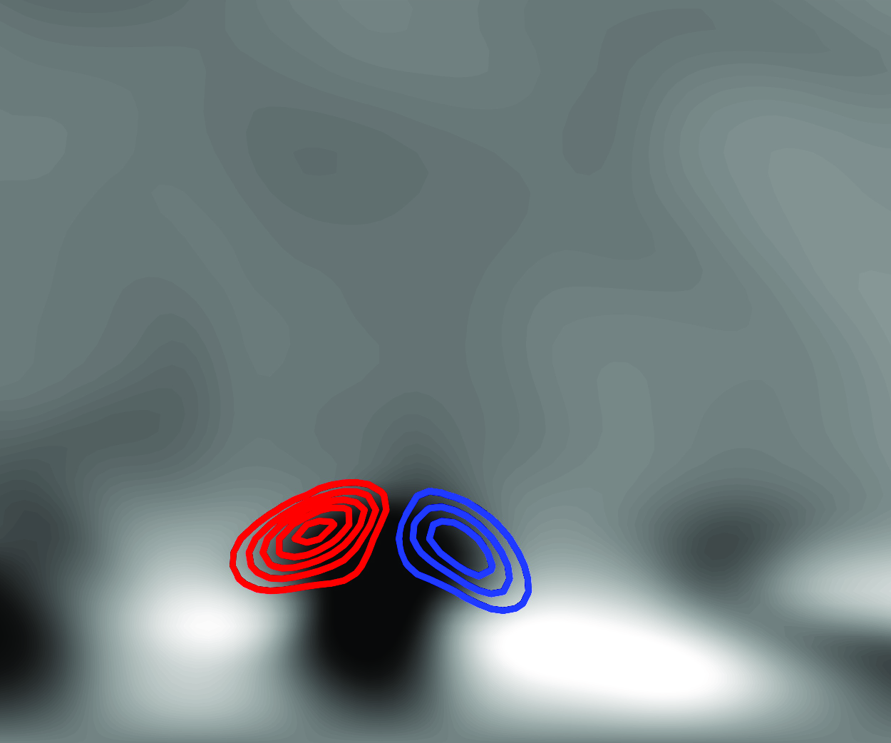
Local stability analysis, described in § 2, was performed for cases 1–4, and the planes under consideration are presented in figure 2. Here, the axes have been normalised by the momentum thickness at
 ${Re}_\theta =116$
, making more clear the spanwise extension difference among the cases and the presence of streaks of various scales. The unstable modes shown in these planes were selected based on the fact that they preceded the nucleation of turbulent spots downstream and at a later time. By comparing the size of these unstable streaks for the different cases, we can see that the actual streak width does not seem to play a significant role regarding stability, with instabilities appearing on streaks of varied sizes.
${Re}_\theta =116$
, making more clear the spanwise extension difference among the cases and the presence of streaks of various scales. The unstable modes shown in these planes were selected based on the fact that they preceded the nucleation of turbulent spots downstream and at a later time. By comparing the size of these unstable streaks for the different cases, we can see that the actual streak width does not seem to play a significant role regarding stability, with instabilities appearing on streaks of varied sizes.

Figure 2. Planes where stability calculations were computed for cases 1 to 4 (top to bottom). The grey contours represent the streamwise velocity perturbations from
 $-0.2$
(black) to
$-0.2$
(black) to
 $0.2$
(white), while the positive (red) and negative (blue) streamwise velocity components of the secondary instability are represented by the open contours. The axes are scaled by the momentum thickness at
$0.2$
(white), while the positive (red) and negative (blue) streamwise velocity components of the secondary instability are represented by the open contours. The axes are scaled by the momentum thickness at
 ${Re}_\theta =116$
.
${Re}_\theta =116$
.
Zoomed views of the unstable modes are included in figure 3, which also includes two adaptions of plots from Hack & Zaki (Reference Hack and Zaki2014) (cf. their figures 6 and 19). These two plots also show the unstable modes on top of the streamwise velocity perturbation from their DNS. The axes have been made non-dimensional by the local momentum thickness
 $\theta _1$
and centred around the secondary instability for better comparison. It can be noted that most of the unstable modes are located on top of a low-speed streak, while only the APG case shows an unstable mode in the shear between a low- and high-speed streak (an inner mode in the terminology adopted in Hack & Zaki (Reference Hack and Zaki2014)). Interestingly, they all exhibit a similar spanwise extension in their local scaling, which seems to be independent of the mode symmetry, either sinuous or varicose, and their streamwise position.
$\theta _1$
and centred around the secondary instability for better comparison. It can be noted that most of the unstable modes are located on top of a low-speed streak, while only the APG case shows an unstable mode in the shear between a low- and high-speed streak (an inner mode in the terminology adopted in Hack & Zaki (Reference Hack and Zaki2014)). Interestingly, they all exhibit a similar spanwise extension in their local scaling, which seems to be independent of the mode symmetry, either sinuous or varicose, and their streamwise position.

Figure 3. Zoomed view of the unstable modes with the axes scaled by the corresponding local momentum thickness
 $\theta _1$
. The colours for cases 1–4 are the same as in figure 2, with the grey solid line indicating the critical layer and the purple markers the perturbation local maxima. The plots for the unstable modes 5 and 6 have been adapted from Hack & Zaki (Reference Hack and Zaki2014).
$\theta _1$
. The colours for cases 1–4 are the same as in figure 2, with the grey solid line indicating the critical layer and the purple markers the perturbation local maxima. The plots for the unstable modes 5 and 6 have been adapted from Hack & Zaki (Reference Hack and Zaki2014).
The spanwise extension of the secondary instabilities can be more clearly seen by computing the energy distribution along the span as
 \begin{equation} E(z) = \int \limits _{0}^{y_{\max }} \hat {\mathbf {u}}^H \hat {\mathbf {u}} \textrm {d}y, \end{equation}
with
 $\hat {\mathbf {u}}=(\hat {u},\hat {v},\hat {w})^{\mathsf {T}}$
and the superscript
$\hat {\mathbf {u}}=(\hat {u},\hat {v},\hat {w})^{\mathsf {T}}$
and the superscript
 $H$
representing the complex conjugate. The energy distribution for the modes in cases 1–4 are shown in figure 4(a), where the curves have been normalised by their corresponding maximum along the span. From this figure, it can be seen that all of them have an extension in the range
$H$
representing the complex conjugate. The energy distribution for the modes in cases 1–4 are shown in figure 4(a), where the curves have been normalised by their corresponding maximum along the span. From this figure, it can be seen that all of them have an extension in the range
 $\approx 8\theta (x)$
–
$\approx 8\theta (x)$
–
 $14\theta (x)$
. Statistical results are included in figure 4(b), showing the distribution of the spanwise width
$14\theta (x)$
. Statistical results are included in figure 4(b), showing the distribution of the spanwise width
 $\Delta z$
of secondary instabilities normalised by the corresponding local momentum thickness. The stability calculations were performed in Faúndez Alarcón et al. (Reference Alarcón, José, Cavalieri, Hanifi and Henningson2024a
), where the flow fields come from the same dataset as case 3 in the present manuscript. In particular, the distribution corresponds to instabilities reaching an
$\Delta z$
of secondary instabilities normalised by the corresponding local momentum thickness. The stability calculations were performed in Faúndez Alarcón et al. (Reference Alarcón, José, Cavalieri, Hanifi and Henningson2024a
), where the flow fields come from the same dataset as case 3 in the present manuscript. In particular, the distribution corresponds to instabilities reaching an
 $N\text {-factor}=3$
and that were connected to nucleation events, with
$N\text {-factor}=3$
and that were connected to nucleation events, with
 $\Delta z$
based on the positions where
$\Delta z$
based on the positions where
 $E(z)$
drops below 1 % of its maximum. Interestingly, most of the instabilities fall in a rather narrow range with a peak around
$E(z)$
drops below 1 % of its maximum. Interestingly, most of the instabilities fall in a rather narrow range with a peak around
 $\approx 13\theta _1$
. As a reference for the streak population range, figure 4(b) also includes the energy distribution of the streaky base flow in case 3 as a function of the spanwise wavelength,
$\approx 13\theta _1$
. As a reference for the streak population range, figure 4(b) also includes the energy distribution of the streaky base flow in case 3 as a function of the spanwise wavelength,
 $\lambda _z$
, at
$\lambda _z$
, at
 $y/\theta _1=3$
. It is worth noting that there is some uncertainty on the streamwise position of the instability, since it corresponds to wave packets convected downstream appearing in a range of streamwise stations and a time window. Therefore, depending on the station where we perform the stability calculation, the scaling can vary slightly and so will the results shown in figure 4.
$y/\theta _1=3$
. It is worth noting that there is some uncertainty on the streamwise position of the instability, since it corresponds to wave packets convected downstream appearing in a range of streamwise stations and a time window. Therefore, depending on the station where we perform the stability calculation, the scaling can vary slightly and so will the results shown in figure 4.

Figure 4. (a) Energy distribution of the unstable modes along the span. The curves correspond to the different cases and are centred at the corresponding modes’ mean position. (b) The black markers show the distribution of instabilities from the same database as case 3. And, as a reference, the energy distribution of the streaky base flow of case 3 at
 $y/\theta _1=3$
is shown in red.
$y/\theta _1=3$
is shown in red.
While the spanwise extension of the secondary instabilities could serve as a good indicator of the size of their hosting streaks, it is not necessarily the most accurate one. This is due mainly to secondary instabilities being localised on top of a distorted low-speed streak, which could lead to an underestimation of the unstable streak wavelength. An alternative approach is to find the local maxima of the streamwise velocity perturbation around the unstable streak, in order to identify the core of the contiguous high-speed streaks. This is shown with the markers on top of the flow fields in figure 3, and noting this is an approximated wavelength since the periodicity along
 $z$
allows only for integer divisions of the domain’s span. By taking the peak-to-peak length, we can estimate the streak wavelength, noting that they are all in the range
$z$
allows only for integer divisions of the domain’s span. By taking the peak-to-peak length, we can estimate the streak wavelength, noting that they are all in the range
 $12{-}15\theta (x)$
, which is, again, independent of the simulation conditions. Particularly, this prevailing spanwise wavelength does not change with the rather large
$12{-}15\theta (x)$
, which is, again, independent of the simulation conditions. Particularly, this prevailing spanwise wavelength does not change with the rather large
 $L_{11}$
range.
$L_{11}$
range.
One natural question that arises when analysing the streaks spacing is how they relate to those that can experience maximum amplification (Andersson et al. Reference Andersson, Berggren and Henningson1999; Luchini Reference Luchini2000). In this context, we compute the optimal energy gain at
 ${Re}_{x_1}$
for stationary disturbances
${Re}_{x_1}$
for stationary disturbances
 $\omega =0$
starting at a prescribed initial position
$\omega =0$
starting at a prescribed initial position
 $x_0$
as
$x_0$
as
 \begin{equation} G(x_1,\beta ) = \max \limits _{\mathbf {u}_0} \frac {\int \mathbf {u}_1^H \mathbf {u}_1 \textrm {d}y}{\int \mathbf {u}_0^H \mathbf {u}_0 \textrm {d}y}, \end{equation}
where
 $\beta$
is the spanwise wavenumber, and, in a slight abuse of notation,
$\beta$
is the spanwise wavenumber, and, in a slight abuse of notation,
 $\mathbf {u}$
corresponds to the perturbation with respect to the time-invariant base flow and not to the secondary instability. The calculations in this case were made non-dimensional by the streamwise position
$\mathbf {u}$
corresponds to the perturbation with respect to the time-invariant base flow and not to the secondary instability. The calculations in this case were made non-dimensional by the streamwise position
 $x_1$
. Figure 5 includes the optimal growth against the spanwise wavelength considering different
$x_1$
. Figure 5 includes the optimal growth against the spanwise wavelength considering different
 $x_0$
for a Blasius boundary layer, the wing profile and, for completeness, it also includes the curves for APG and favourable pressure gradient (FPG) considering the Hartree parameter
$x_0$
for a Blasius boundary layer, the wing profile and, for completeness, it also includes the curves for APG and favourable pressure gradient (FPG) considering the Hartree parameter
 $\beta _H=-0.14$
and
$\beta _H=-0.14$
and
 $\beta _H=0.14$
, respectively. Due to the Reynolds independence characteristic of the Blasius boundary layer for optimal growth (Andersson et al. Reference Andersson, Berggren and Henningson1999), the corresponding plot is valid for all ZPG cases under study. On the other hand, the optimal results for the wing are specific for this particular case and
$\beta _H=0.14$
, respectively. Due to the Reynolds independence characteristic of the Blasius boundary layer for optimal growth (Andersson et al. Reference Andersson, Berggren and Henningson1999), the corresponding plot is valid for all ZPG cases under study. On the other hand, the optimal results for the wing are specific for this particular case and
 ${Re}_{x_1}$
. The lines associated with
${Re}_{x_1}$
. The lines associated with
 $x_0=0.01$
can be directly contrasted against the results in Andersson et al. (Reference Andersson, Berggren and Henningson1999) and Faúndez Alarcón et al. (Reference Alarcón, José, Morra, Hanifi and Henningson2022), for Blasius and the wing boundary layer, respectively. These are related to linear receptivity mechanisms, where the perturbations penetrate the boundary layer close to the leading edge (Brandt et al. Reference Brandt, Henningson and Ponziani2002) to then grow according to their optimal component. The interpretation of larger values of
$x_0=0.01$
can be directly contrasted against the results in Andersson et al. (Reference Andersson, Berggren and Henningson1999) and Faúndez Alarcón et al. (Reference Alarcón, José, Morra, Hanifi and Henningson2022), for Blasius and the wing boundary layer, respectively. These are related to linear receptivity mechanisms, where the perturbations penetrate the boundary layer close to the leading edge (Brandt et al. Reference Brandt, Henningson and Ponziani2002) to then grow according to their optimal component. The interpretation of larger values of
 $x_0$
is less clear, but they can be related to nonlinearly generated perturbations in the boundary layer that will nonetheless grow due to linear mechanisms (Schmid & Henningson Reference Schmid and Henningson2001). Interestingly, when optimal initial perturbations are placed closer to the objective position there is a shift towards shorter wavelengths that can reach higher amplification. This behaviour is much more pronounced in the optimal growth corresponding to the wing.
$x_0$
is less clear, but they can be related to nonlinearly generated perturbations in the boundary layer that will nonetheless grow due to linear mechanisms (Schmid & Henningson Reference Schmid and Henningson2001). Interestingly, when optimal initial perturbations are placed closer to the objective position there is a shift towards shorter wavelengths that can reach higher amplification. This behaviour is much more pronounced in the optimal growth corresponding to the wing.

Figure 5. Optimal growth vs spanwise wavelength
 $\lambda _z$
for different initial positions
$\lambda _z$
for different initial positions
 $x_0$
. The wavelength has been made non-dimensional by the local momentum thickness at the objective position.
$x_0$
. The wavelength has been made non-dimensional by the local momentum thickness at the objective position.
When comparing the results shown in figure 5 with the peak-to-peak spacing in figure 3, we can see that the breaking streaks are in the range of those reaching maximum amplification. In this type of transition scenario, with a broadband disturbance spectrum, the optimal amplification could explain why it is within this range that breaking streaks are more likely to be found. There is, of course, an intricate interplay between energy transfer and optimal growth that will set the streak spacing in the boundary layer, and which is largely dependent on the inflow FST conditions. While small spanwise wavenumbers (large wavelengths) will reach maximum amplification downstream in the boundary layer, the preferred energy propagation towards higher wavenumber through the
 $\beta$
-cascade (Henningson et al. Reference Henningson, Lundbladh and Johansson1993) can give rise to shorter spanwise wavelength able to reach maximum amplification upstream, even when they were not initially present in the incoming FST. Unlike linear receptivity, the nonlinear interactions responsible for the energy transfer can take place throughout the boundary layer, profiting from the optimal growth that downstream induced perturbations can achieve, as shown in figure 5.
$\beta$
-cascade (Henningson et al. Reference Henningson, Lundbladh and Johansson1993) can give rise to shorter spanwise wavelength able to reach maximum amplification upstream, even when they were not initially present in the incoming FST. Unlike linear receptivity, the nonlinear interactions responsible for the energy transfer can take place throughout the boundary layer, profiting from the optimal growth that downstream induced perturbations can achieve, as shown in figure 5.
4. Concluding remarks
In this work, we have collected the stability analysis of streaky flows in boundary layers for six different numerical simulations. The main purpose of this survey is to provide numerical evidence from well-resolved simulations of bypass transition regarding the spanwise spacing of the streak secondary instabilities and their hosting streaks. We have observed that independently of the geometry, FST conditions and streamwise positions, the spacing of the breaking streaks is in a rather narrow range when scaled by the local momentum thickness. This is particularly remarkable after noting the large variation in the integral length scale among the cases. Although figure 4 provides statistical support for our main conclusion in one of the cases, it is reasonable to assume that it holds for the other cases as well, in particular since the shape of the streaks, their streamwise development and the characteristics of their secondary instability is the same in all cases.
We provide a plausible explanation for the seeming preference of a specific wavelength for breaking streaks. Through optimal disturbance theory, we show that this spanwise wavelength of
 $12{-}15\theta (x)$
is within the range of streaks that can reach maximum amplification. The question regarding the causality of optimal amplification on streak instabilities remains open, since the latter might respond to various streak properties other than only their amplitude, as suggested, for instance, by Hack & Zaki (Reference Hack and Zaki2016). However, the fact that maximum transient growth is achieved within this range could explain, at least, why streaks around this width are more likely to be seen breaking down.
$12{-}15\theta (x)$
is within the range of streaks that can reach maximum amplification. The question regarding the causality of optimal amplification on streak instabilities remains open, since the latter might respond to various streak properties other than only their amplitude, as suggested, for instance, by Hack & Zaki (Reference Hack and Zaki2016). However, the fact that maximum transient growth is achieved within this range could explain, at least, why streaks around this width are more likely to be seen breaking down.
The emergence of breaking streaks with a specific wavelength due to their optimal growth could serve as a basis for the hypothesis posed by Fransson & Shahinfar (Reference Fransson and Shahinfar2020) about the existence of an optimal ratio between
 $L_{11}$
and boundary-layer thickness at transition. By recognising the role of
$L_{11}$
and boundary-layer thickness at transition. By recognising the role of
 $L_{11}$
in distributing the energy along the spectrum, it is then reasonable that there exists an optimal distribution such that the necessary streak amplification is achieved closest to the leading edge through their optimal growth. Such an optimisation problem, however, should consider not only the optimal growth but also the energy transfer taking place along the boundary layer.
$L_{11}$
in distributing the energy along the spectrum, it is then reasonable that there exists an optimal distribution such that the necessary streak amplification is achieved closest to the leading edge through their optimal growth. Such an optimisation problem, however, should consider not only the optimal growth but also the energy transfer taking place along the boundary layer.
The twofold effect of
 $L_{11}$
observed experimentally by Fransson & Shahinfar (Reference Fransson and Shahinfar2020) and corroborated numerically by Durović et al. (Reference Durović, Hanifi, Schlatter, Sasaki and Henningson2024) is also consistent with the ideas shown here. The observation that increasing
$L_{11}$
observed experimentally by Fransson & Shahinfar (Reference Fransson and Shahinfar2020) and corroborated numerically by Durović et al. (Reference Durović, Hanifi, Schlatter, Sasaki and Henningson2024) is also consistent with the ideas shown here. The observation that increasing
 $L_{11}$
could also delay transition can be understood by noting that a very low wavenumber will reach maximum amplification farther downstream. This would make their breakdown unlikely, where a more likely breakdown will take place due to energy transfer through the
$L_{11}$
could also delay transition can be understood by noting that a very low wavenumber will reach maximum amplification farther downstream. This would make their breakdown unlikely, where a more likely breakdown will take place due to energy transfer through the
 $\beta$
-cascade to a higher wavenumber that can actually grow at upstream positions. The lower the initial wavenumber, the slower their amplification will be, and therefore the longer it will take for the nonlinearities to propagate energy.
$\beta$
-cascade to a higher wavenumber that can actually grow at upstream positions. The lower the initial wavenumber, the slower their amplification will be, and therefore the longer it will take for the nonlinearities to propagate energy.
Acknowledgments
The original authors of the various data sets used in this work are gratefully acknowledged. The computations were performed on resources provided by The National Academic Infrastructure for Supercomputing in Sweden (NAISS) at PDC and NSC.
Funding
This work was funded by Vinnova through the NFFP project LaFloDes (grant number 2019-05369); the European Research Council (grant agreement 694452-TRANSEP-ERC-2015-AdG); and the Swedish e-Science Research Centre (SeRC).
Declaration of interests
The authors report no conflict of interest.


 Open access