1 Introduction
Simultaneous shear and buoyancy are ubiquitous in many engineering and geophysical turbulent flows such as density-driven boundary layers in the ocean (Keitzl, Mellado & Notz Reference Keitzl, Mellado and Notz2016), air flow over land surfaces and ice sheets (Fernando & Weil Reference Fernando and Weil2010; Katul, Konings & Porporato Reference Katul, Konings and Porporato2011; Mahrt Reference Mahrt2014) and flows in heat exchangers (You, Yoo & Choi Reference You, Yoo and Choi2003). Buoyancy complicates the flow dynamics beyond the well-studied canonical turbulent boundary layer, resulting in a rich set of persistent intellectual challenges. The ratio of the buoyant to inertial forces can be computed to assess their relative roles. This ratio is usually denoted as a Richardson number (
 $Ri$
, many formulations exist as detailed for example in Stull (Reference Stull1988)). An
$Ri$
, many formulations exist as detailed for example in Stull (Reference Stull1988)). An
 $Ri=0$
indicates no buoyancy effect, while a very large
$Ri=0$
indicates no buoyancy effect, while a very large
 $Ri$
magnitude indicates a buoyancy-dominated flow. Buoyancy can either augment turbulence generation in unstable flows (
$Ri$
magnitude indicates a buoyancy-dominated flow. Buoyancy can either augment turbulence generation in unstable flows (
 $Ri<0$
) (Chauhan et al.
Reference Chauhan, Hutchins, Monty and Marusic2012; Salesky, Chamecki & Bou-Zeid Reference Salesky, Chamecki and Bou-Zeid2017), or transfer turbulent kinetic energy (TKE) into potential energy associated with the variance of the density field in stable flows (
$Ri<0$
) (Chauhan et al.
Reference Chauhan, Hutchins, Monty and Marusic2012; Salesky, Chamecki & Bou-Zeid Reference Salesky, Chamecki and Bou-Zeid2017), or transfer turbulent kinetic energy (TKE) into potential energy associated with the variance of the density field in stable flows (
 $Ri>0$
) (Zilitinkevich Reference Zilitinkevich2002; Karimpour & Venayagamoorthy Reference Karimpour and Venayagamoorthy2015; Venayagamoorthy & Koseff Reference Venayagamoorthy and Koseff2016). In the two limits where buoyancy dominates,
$Ri>0$
) (Zilitinkevich Reference Zilitinkevich2002; Karimpour & Venayagamoorthy Reference Karimpour and Venayagamoorthy2015; Venayagamoorthy & Koseff Reference Venayagamoorthy and Koseff2016). In the two limits where buoyancy dominates,
 $Ri\ll 0$
indicates a regime of natural (free) convection (Mellado Reference Mellado2012), while laminarization (full or intermittent as shown in Ansorge & Mellado (Reference Ansorge and Mellado2014), Mahrt (Reference Mahrt2014), Shah & Bou-Zeid (Reference Shah and Bou-Zeid2014a
)) can occur when
$Ri\ll 0$
indicates a regime of natural (free) convection (Mellado Reference Mellado2012), while laminarization (full or intermittent as shown in Ansorge & Mellado (Reference Ansorge and Mellado2014), Mahrt (Reference Mahrt2014), Shah & Bou-Zeid (Reference Shah and Bou-Zeid2014a
)) can occur when
 $Ri\gg 0$
. The transitions with
$Ri\gg 0$
. The transitions with
 $Ri$
between these two limiting stability regimes are nonlinear in terms of the influence on turbulence intensity and variance isotropy, and on the structural characteristics of eddies (i.e. their evolution from pancake-like horizontal motions under very-stable conditions, to hairpins and hairpin packets under near-neutral stability, to thermals and plumes under free convection).
$Ri$
between these two limiting stability regimes are nonlinear in terms of the influence on turbulence intensity and variance isotropy, and on the structural characteristics of eddies (i.e. their evolution from pancake-like horizontal motions under very-stable conditions, to hairpins and hairpin packets under near-neutral stability, to thermals and plumes under free convection).
A hallmark of flows bounded by a horizontal wall is the misalignment of shear production of turbulence in the streamwise direction and buoyancy production or destruction in the wall-normal direction. The energy exchanges between the components and the complex feedbacks across various statistical moments of the velocity and density fields give rise to counter-intuitive results. Buoyancy simultaneously influences the TKE budget of the flow and the effectiveness of eddies in transporting heat and momentum (Li & Bou-Zeid Reference Li and Bou-Zeid2011; Shah & Bou-Zeid Reference Shah and Bou-Zeid2014b ). Furthermore, while buoyancy acts on the wall-normal component, numerical simulations confirm that its primary impact in statically stable flows is through the reduction in horizontal velocity-variance shear production that buoyancy instigates indirectly (Jacobitz, Sarkar & VanAtta Reference Jacobitz, Sarkar and Vanatta1997; Shah & Bou-Zeid Reference Shah and Bou-Zeid2014a ).
How does buoyancy alter the energy exchanges between the different components, and what are the implications for the dynamics of wall-bounded turbulent flows are the questions that frame this work. In the next section, we will overview the basic model development, followed in § 3 by validation of the results and discussion of their key implications on buoyancy modulation of turbulence. In § 4, we extend the model using the simplest energy redistribution closure framework to further probe the role of the interaction between redistribution and buoyancy on variance budgets and anisotropy. We then conclude with a summary and discussion of the broader implications of the findings.
2 Reduced model development
The budget equations for the variances of individual turbulent velocity components reveal the exchange of kinetic energy through the ‘pressure redistribution’ terms. These terms, as their alternative ‘return to isotropy’ name indicates, nudge turbulence towards an isotropic state where its kinetic energy would be equipartitioned among its three velocity components (the redistribution terms sum exactly to zero in incompressible flows and thus do not appear in the equation for the full TKE budget). However, when TKE production in one or two of the components dominate, the flow cannot reach such an isotropic state except at scales commensurate with the Kolmogorov microscale
 $\unicode[STIX]{x1D702}_{K}$
(provided
$\unicode[STIX]{x1D702}_{K}$
(provided
 $\unicode[STIX]{x1D702}_{K}\ll$
than the Dougherty–Ozmidov scale (Dougherty Reference Dougherty1961) so that the anisotropic influence of buoyancy at these small scales is negligible). The degree of anisotropy therefore depends on the interplay between the anisotropic production by shear or buoyancy and the effectiveness of the redistribution process that acts differently across scales of motion (Brugger et al.
Reference Brugger, Katul, De Roo, Kröniger, Rotenberg, Rohatyn and Mauder2018). It is therefore reasonable to hypothesize that these return-to-isotropy terms encode significant information about the statistical and structural properties of the turbulent velocity, and how such properties are modulated by the shear-to-buoyancy balance encoded in
$\unicode[STIX]{x1D702}_{K}\ll$
than the Dougherty–Ozmidov scale (Dougherty Reference Dougherty1961) so that the anisotropic influence of buoyancy at these small scales is negligible). The degree of anisotropy therefore depends on the interplay between the anisotropic production by shear or buoyancy and the effectiveness of the redistribution process that acts differently across scales of motion (Brugger et al.
Reference Brugger, Katul, De Roo, Kröniger, Rotenberg, Rohatyn and Mauder2018). It is therefore reasonable to hypothesize that these return-to-isotropy terms encode significant information about the statistical and structural properties of the turbulent velocity, and how such properties are modulated by the shear-to-buoyancy balance encoded in
 $Ri$
. Buoyancy damping or excitation of vertical velocity must be communicated by these terms to the horizontal directions.
$Ri$
. Buoyancy damping or excitation of vertical velocity must be communicated by these terms to the horizontal directions.
A logical starting point is an idealized high Reynolds number flow that remains three-dimensional with finite TKE in all components. A statistically steady state is assumed, which in geophysical settings must be interpreted as steadiness over limited periods, e.g. 15–60 min in the lower atmosphere (Stull Reference Stull1988; Salesky, Chamecki & Dias Reference Salesky, Chamecki and Dias2012). Over a horizontally homogeneous wall, the flow will also be statistically homogeneous over the streamwise and cross-stream directions, which for an incompressible flow also results in negligible mean vertical velocity. We will neglect the terms in the variance budgets that result from rotation (the Coriolis force) since they are of second-order importance (Stull Reference Stull1988); the effect of the Coriolis force mainly manifests as a rotation of the mean flow. The vertical TKE-transport terms are significant in the viscous and buffer layers, and also potentially in the outer layer (Pope Reference Pope2000), but if one is interested in the inertial sublayer (the logarithmic region), the transport terms are approximately one order of magnitude smaller than the production and dissipation terms and can be neglected in a reduced model (André et al. Reference André, De Moor, Lacarrère and du Vachat1978; Pope Reference Pope2000; Shah & Bou-Zeid Reference Shah and Bou-Zeid2014a ; Momen & Bou-Zeid Reference Momen and Bou-Zeid2017). This assumption might break down under strong wall buoyancy flux or near the density inversion that typically delineates the top of the atmospheric boundary layer (Stull Reference Stull1988; Garcia & Mellado Reference Garcia and Mellado2014), but will be adopted here since it is reasonable in the logarithmic layer under a wide range of stabilities (see appendix A for a model derivation where these terms are retained). An important side note to highlight is that, unlike for kinetic energy, the transport of density (or equivalently potential temperature) fluctuations is usually not negligible, and as a result the production–dissipation balance does not apply to scalar variance (Karimpour & Venayagamoorthy Reference Karimpour and Venayagamoorthy2015) and is not invoked here.
In summary, a high-
 $Re$
planar–homogeneous steady flow with an equilibrium between TKE production (by shear and buoyancy) and dissipation (by viscosity and buoyancy) is postulated. Such an idealization is in fact quite routinely used in practice when interpreting measurements in the inertial turbulent sublayer in laboratory experiments or flux measurements in the all-important atmospheric surface layer, or when collapsing field experiments in the context of Monin–Obukhov similarity theory (MOST) (Monin & Obukhov Reference Monin and Obukhov1954; Kader & Yaglom Reference Kader and Yaglom1990; Foken Reference Foken2006; Bou-Zeid et al.
Reference Bou-Zeid, Higgins, Huwald, Meneveau and Parlange2010; Ghannam et al.
Reference Ghannam, Katul, Bou-Zeid, Gerken and Chamecki2018; Li, Katul & Liu Reference Li, Katul and Liu2018). With these assumptions, the velocity half-variance budgets reduce to (Zilitinkevich Reference Zilitinkevich1973; Stull Reference Stull1988):
$Re$
planar–homogeneous steady flow with an equilibrium between TKE production (by shear and buoyancy) and dissipation (by viscosity and buoyancy) is postulated. Such an idealization is in fact quite routinely used in practice when interpreting measurements in the inertial turbulent sublayer in laboratory experiments or flux measurements in the all-important atmospheric surface layer, or when collapsing field experiments in the context of Monin–Obukhov similarity theory (MOST) (Monin & Obukhov Reference Monin and Obukhov1954; Kader & Yaglom Reference Kader and Yaglom1990; Foken Reference Foken2006; Bou-Zeid et al.
Reference Bou-Zeid, Higgins, Huwald, Meneveau and Parlange2010; Ghannam et al.
Reference Ghannam, Katul, Bou-Zeid, Gerken and Chamecki2018; Li, Katul & Liu Reference Li, Katul and Liu2018). With these assumptions, the velocity half-variance budgets reduce to (Zilitinkevich Reference Zilitinkevich1973; Stull Reference Stull1988):
 $$\begin{eqnarray}\displaystyle & \displaystyle -\overline{u^{\prime }w^{\prime }}\frac{\unicode[STIX]{x2202}\overline{u}}{\unicode[STIX]{x2202}z}+\overline{\frac{p^{\prime }}{\unicode[STIX]{x1D70C}_{r}}\frac{\unicode[STIX]{x2202}u^{\prime }}{\unicode[STIX]{x2202}x}}-\unicode[STIX]{x1D708}\overline{\left(\frac{\unicode[STIX]{x2202}u^{\prime }}{\unicode[STIX]{x2202}x_{j}}\right)^{2}}=S+R_{u}-\unicode[STIX]{x1D700}_{u}=0, & \displaystyle\end{eqnarray}$$
 $$\begin{eqnarray}\displaystyle & \displaystyle \overline{\frac{p^{\prime }}{\unicode[STIX]{x1D70C}_{r}}\frac{\unicode[STIX]{x2202}v^{\prime }}{\unicode[STIX]{x2202}y}}-\unicode[STIX]{x1D708}\overline{\left(\frac{\unicode[STIX]{x2202}v^{\prime }}{\unicode[STIX]{x2202}x_{j}}\right)^{2}}=R_{v}-\unicode[STIX]{x1D700}_{v}=0, & \displaystyle\end{eqnarray}$$
 $$\begin{eqnarray}\displaystyle & \displaystyle -\frac{g}{\unicode[STIX]{x1D70C}_{r}}\overline{w^{\prime }\unicode[STIX]{x1D70C}^{\prime }}+\overline{\frac{p^{\prime }}{\unicode[STIX]{x1D70C}_{r}}\frac{\unicode[STIX]{x2202}w^{\prime }}{\unicode[STIX]{x2202}z}}-\unicode[STIX]{x1D708}\overline{\left(\frac{\unicode[STIX]{x2202}w^{\prime }}{\unicode[STIX]{x2202}x_{j}}\right)^{2}}=B+R_{w}-\unicode[STIX]{x1D700}_{w}=0. & \displaystyle\end{eqnarray}$$
Throughout,
 $u,v,w$
indicate instantaneous velocity components in the streamwise (
$u,v,w$
indicate instantaneous velocity components in the streamwise (
 $x$
), cross-stream (
$x$
), cross-stream (
 $y$
) and vertical (
$y$
) and vertical (
 $z$
) directions, respectively;
$z$
) directions, respectively;
 $p$
is instantaneous pressure;
$p$
is instantaneous pressure;
 $\unicode[STIX]{x1D70C}$
is density and
$\unicode[STIX]{x1D70C}$
is density and
 $\unicode[STIX]{x1D70C}_{r}$
its reference value; and
$\unicode[STIX]{x1D70C}_{r}$
its reference value; and
 $\unicode[STIX]{x1D708}$
is kinematic viscosity. Instantaneous quantities are decomposed into their turbulent fluctuations, denoted by a prime, and their averaged states, denoted by an overbar, where averaging is performed over coordinates of statistical homogeneity. The symbols in the middle equations refer, in the same order, to the terms on the left-hand side. The first term on the left-hand side of (2.1) is shear production
$\unicode[STIX]{x1D708}$
is kinematic viscosity. Instantaneous quantities are decomposed into their turbulent fluctuations, denoted by a prime, and their averaged states, denoted by an overbar, where averaging is performed over coordinates of statistical homogeneity. The symbols in the middle equations refer, in the same order, to the terms on the left-hand side. The first term on the left-hand side of (2.1) is shear production
 $(S>0)$
, while in (2.3) the first term is buoyancy production (
$(S>0)$
, while in (2.3) the first term is buoyancy production (
 $B>0$
) or destruction (
$B>0$
) or destruction (
 $B<0$
). The terms with
$B<0$
). The terms with
 $p$
are pressure redistribution terms (denoted by
$p$
are pressure redistribution terms (denoted by
 $R_{u}$
,
$R_{u}$
,
 $R_{v}$
and
$R_{v}$
and
 $R_{w}$
), and the last terms on the left-hand side are viscous dissipation rates (
$R_{w}$
), and the last terms on the left-hand side are viscous dissipation rates (
 $\unicode[STIX]{x1D700}_{u}$
,
$\unicode[STIX]{x1D700}_{u}$
,
 $\unicode[STIX]{x1D700}_{v}$
and
$\unicode[STIX]{x1D700}_{v}$
and
 $\unicode[STIX]{x1D700}_{w}$
, all positive).
$\unicode[STIX]{x1D700}_{w}$
, all positive).
The dissipation is performed by viscosity acting on the smallest eddies commensurate in size to
 $\unicode[STIX]{x1D702}_{K}$
. If
$\unicode[STIX]{x1D702}_{K}$
. If
 $Re$
is sufficiently high, the energy cascade dissipates the anisotropy injected at the largest scales, resulting in an approximately isotropic dissipation with
$Re$
is sufficiently high, the energy cascade dissipates the anisotropy injected at the largest scales, resulting in an approximately isotropic dissipation with
 $$\begin{eqnarray}\unicode[STIX]{x1D700}_{u}=\unicode[STIX]{x1D700}_{v}=\unicode[STIX]{x1D700}_{w}\quad \Rightarrow \quad \unicode[STIX]{x1D700}_{w}+\unicode[STIX]{x1D700}_{v}=2\unicode[STIX]{x1D700}_{u}.\end{eqnarray}$$
Viscous-range isotropy might not be exact at moderate
 $Re$
where the limited turnovers between the production and dissipation do not completely remove the signature of the large-scale anisotropy. An anisotropy factor could then be introduced to generalize the model. However, under sufficiently high
$Re$
where the limited turnovers between the production and dissipation do not completely remove the signature of the large-scale anisotropy. An anisotropy factor could then be introduced to generalize the model. However, under sufficiently high
 $Re$
and ‘far’ from any wall effect (i.e. outside the buffer layer), the difference between the three components of dissipation and their mean is less than 10% (Spalart Reference Spalart1988; Pope Reference Pope2000) and is ignored here. Another potential source of viscous-range anisotropy is strong static stability at high
$Re$
and ‘far’ from any wall effect (i.e. outside the buffer layer), the difference between the three components of dissipation and their mean is less than 10% (Spalart Reference Spalart1988; Pope Reference Pope2000) and is ignored here. Another potential source of viscous-range anisotropy is strong static stability at high
 $Ri$
where the Dougherty–Ozmidov length scale decreases and could become
$Ri$
where the Dougherty–Ozmidov length scale decreases and could become
 ${\sim}\unicode[STIX]{x1D702}_{K}$
(Grachev et al.
Reference Grachev, Andreas, Fairall, Guest and Persson2015; Li, Salesky & Banerjee Reference Li, Salesky and Banerjee2016); this aspect will be analysed in future studies using direct numerical simulation data.
${\sim}\unicode[STIX]{x1D702}_{K}$
(Grachev et al.
Reference Grachev, Andreas, Fairall, Guest and Persson2015; Li, Salesky & Banerjee Reference Li, Salesky and Banerjee2016); this aspect will be analysed in future studies using direct numerical simulation data.
Equations (2.1)–(2.3) are combined with (2.4) to yield
 $$\begin{eqnarray}B+R_{w}+R_{v}=2S+2R_{u}.\end{eqnarray}$$
In addition, since the redistribution terms must sum to zero in an incompressible flow,
 $$\begin{eqnarray}R_{u}+R_{v}+R_{w}=0\quad \Rightarrow \quad R_{v}+R_{w}=-R_{u}.\end{eqnarray}$$
Replacing (2.6) into (2.5), dividing by
 $S$
and noting that
$S$
and noting that
 $-B/S=Ri_{f}$
yields
$-B/S=Ri_{f}$
yields
 $$\begin{eqnarray}\frac{R_{u}}{S}=-\frac{2}{3}-\frac{1}{3}Ri_{f}.\end{eqnarray}$$
In a similar fashion, equations (2.4)–(2.6) can be modified (writing
 $\unicode[STIX]{x1D700}_{u}+\unicode[STIX]{x1D700}_{w}=2\unicode[STIX]{x1D700}_{v}$
in (2.4) and
$\unicode[STIX]{x1D700}_{u}+\unicode[STIX]{x1D700}_{w}=2\unicode[STIX]{x1D700}_{v}$
in (2.4) and
 $R_{u}+R_{w}=-R_{v}$
in (2.6)) to yield
$R_{u}+R_{w}=-R_{v}$
in (2.6)) to yield
 $$\begin{eqnarray}\frac{R_{v}}{S}=\frac{1}{3}-\frac{1}{3}Ri_{f}.\end{eqnarray}$$
Then, using
 $R_{w}=-R_{u}-R_{v}$
results in
$R_{w}=-R_{u}-R_{v}$
results in
 $$\begin{eqnarray}\frac{R_{w}}{S}=\frac{1}{3}+\frac{2}{3}Ri_{f}.\end{eqnarray}$$
Finally, the total TKE dissipation
 $\unicode[STIX]{x1D700}$
(the sum of the half-variance dissipations in all three components that is used to define
$\unicode[STIX]{x1D700}$
(the sum of the half-variance dissipations in all three components that is used to define
 $\unicode[STIX]{x1D702}_{K}=(\unicode[STIX]{x1D708}^{3}/\unicode[STIX]{x1D700})^{1/4}$
) can be related to
$\unicode[STIX]{x1D702}_{K}=(\unicode[STIX]{x1D708}^{3}/\unicode[STIX]{x1D700})^{1/4}$
) can be related to
 $Ri_{f}$
by summing (2.1) to (2.3), and using (2.6), to obtain
$Ri_{f}$
by summing (2.1) to (2.3), and using (2.6), to obtain
 $$\begin{eqnarray}\frac{\unicode[STIX]{x1D700}_{u}+\unicode[STIX]{x1D700}_{v}+\unicode[STIX]{x1D700}_{w}}{S}=\frac{\unicode[STIX]{x1D700}}{S}=1-Ri_{f}.\end{eqnarray}$$
3 Validation and implications
Equations (2.7)–(2.10) constitute a basic ‘reduced model’ that describes how energy redistribution and dissipation change with
 $Ri_{f}$
. Under neutral conditions where
$Ri_{f}$
. Under neutral conditions where
 $Ri_{f}=0$
, the model assumptions and formulation are very similar to algebraic Reynolds stress models such as those proposed by Launder, Reece & Rodi (Reference Launder, Reece and Rodi1975) (see also Pope (Reference Pope2000), § 11.9). In this neutral limit, the model predicts
$Ri_{f}=0$
, the model assumptions and formulation are very similar to algebraic Reynolds stress models such as those proposed by Launder, Reece & Rodi (Reference Launder, Reece and Rodi1975) (see also Pope (Reference Pope2000), § 11.9). In this neutral limit, the model predicts
 $R_{u}=-2S/3$
and
$R_{u}=-2S/3$
and
 $R_{v}=R_{w}=S/3$
. This yields the expected result that two thirds of shear production in the
$R_{v}=R_{w}=S/3$
. This yields the expected result that two thirds of shear production in the
 $u$
component is redistributed equally into the
$u$
component is redistributed equally into the
 $v$
and
$v$
and
 $w$
components where they are dissipated via
$w$
components where they are dissipated via
 $\unicode[STIX]{x1D700}_{v}=\unicode[STIX]{x1D700}_{w}$
, and that one third of shear production gets dissipated directly via
$\unicode[STIX]{x1D700}_{v}=\unicode[STIX]{x1D700}_{w}$
, and that one third of shear production gets dissipated directly via
 $\unicode[STIX]{x1D700}_{u}$
. This outcome results in equal energy in the cross-stream and vertical components, which is not observed in wall-bounded flows (Stull Reference Stull1988; Bou-Zeid, Meneveau & Parlange Reference Bou-Zeid, Meneveau and Parlange2005) due to the influence of the mean shear and to the wall pressure-blockage effect (McColl et al.
Reference McColl, Katul, Gentine and Entekhabi2016) that is absent here. The effect of this wall blockage is to increase pressure (
$\unicode[STIX]{x1D700}_{u}$
. This outcome results in equal energy in the cross-stream and vertical components, which is not observed in wall-bounded flows (Stull Reference Stull1988; Bou-Zeid, Meneveau & Parlange Reference Bou-Zeid, Meneveau and Parlange2005) due to the influence of the mean shear and to the wall pressure-blockage effect (McColl et al.
Reference McColl, Katul, Gentine and Entekhabi2016) that is absent here. The effect of this wall blockage is to increase pressure (
 $p^{\prime }>0$
) for descending parcels (
$p^{\prime }>0$
) for descending parcels (
 $\unicode[STIX]{x2202}w^{\prime }/\unicode[STIX]{x2202}z<0$
since
$\unicode[STIX]{x2202}w^{\prime }/\unicode[STIX]{x2202}z<0$
since
 $w=0$
at the wall), while decreasing pressure (
$w=0$
at the wall), while decreasing pressure (
 $p^{\prime }<0$
) for ascending parcels (
$p^{\prime }<0$
) for ascending parcels (
 $\unicode[STIX]{x2202}w^{\prime }\unicode[STIX]{x2202}z>0$
). Wall blockage thus consistently produces negative (
$\unicode[STIX]{x2202}w^{\prime }\unicode[STIX]{x2202}z>0$
). Wall blockage thus consistently produces negative (
 $p^{\prime }\unicode[STIX]{x2202}w^{\prime }/\unicode[STIX]{x2202}z$
) contributions, or reduces the magnitude of the positive contributions, and as a result reduces the magnitude of the average redistribution of energy into the
$p^{\prime }\unicode[STIX]{x2202}w^{\prime }/\unicode[STIX]{x2202}z$
) contributions, or reduces the magnitude of the positive contributions, and as a result reduces the magnitude of the average redistribution of energy into the
 $w$
component,
$w$
component,
 $\overline{p^{\prime }\unicode[STIX]{x2202}w^{\prime }/\unicode[STIX]{x2202}z}>0$
, below model predictions. The comparative influence of wall blockage relative to the influence of increasing shear in the vicinity of the wall is discussed in Launder et al. (Reference Launder, Reece and Rodi1975).
$\overline{p^{\prime }\unicode[STIX]{x2202}w^{\prime }/\unicode[STIX]{x2202}z}>0$
, below model predictions. The comparative influence of wall blockage relative to the influence of increasing shear in the vicinity of the wall is discussed in Launder et al. (Reference Launder, Reece and Rodi1975).
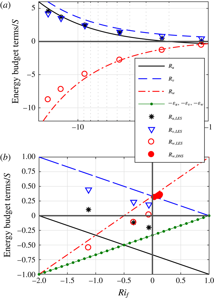
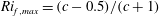
To assess the impact of neglecting wall blockage and other assumptions, the redistribution terms normalized by shear production (2.7)–(2.9) are compared to results from large eddy simulation (LES) under unstable conditions (
 $Ri_{f}<0$
) and direct numerical simulation (DNS) under stable conditions (
$Ri_{f}<0$
) and direct numerical simulation (DNS) under stable conditions (
 $Ri_{f}>0$
). The DNS and LES details, with further references, are respectively provided in appendices B and C. It is noted that (i) the pressure redistribution terms are difficult to measure experimentally (no such measurements have been reported in the literature) and thus simulations are the only avenue for estimating them, and (ii) due to subgrid-scale modelling in the LES, these computations are deemed less accurate than in DNS. For the LES and DNS, the vertical average of the redistribution terms and of
$Ri_{f}>0$
). The DNS and LES details, with further references, are respectively provided in appendices B and C. It is noted that (i) the pressure redistribution terms are difficult to measure experimentally (no such measurements have been reported in the literature) and thus simulations are the only avenue for estimating them, and (ii) due to subgrid-scale modelling in the LES, these computations are deemed less accurate than in DNS. For the LES and DNS, the vertical average of the redistribution terms and of
 $Ri_{f}$
over the inertial sublayer (logarithmic or modified logarithmic if non-neutral) are taken for comparisons since this is the layer where our model assumptions hold and that is of most interest in high-
$Ri_{f}$
over the inertial sublayer (logarithmic or modified logarithmic if non-neutral) are taken for comparisons since this is the layer where our model assumptions hold and that is of most interest in high-
 $Re$
flows. The three redistribution terms computed from the reduced model and from the simulations are compared in figure 1. Figure 1(a) is for strongly unstable conditions (
$Re$
flows. The three redistribution terms computed from the reduced model and from the simulations are compared in figure 1. Figure 1(a) is for strongly unstable conditions (
 $Ri_{f}<-1$
) and shows that the model captures LES trends but with some discrepancies. Figure 1(b) is for moderately unstable to stable conditions (
$Ri_{f}<-1$
) and shows that the model captures LES trends but with some discrepancies. Figure 1(b) is for moderately unstable to stable conditions (
 $-2<Ri_{f}<1$
), where the model again reasonably reproduces LES trends, but the relative errors are larger than for the strongly unstable conditions. The agreement with DNS is significantly better. These DNS were of rotating (Ekman) flows where the two horizontal-variance components are difficult to disentangle due to shear production in the cross-stream direction. Here, they are lumped and compared to
$-2<Ri_{f}<1$
), where the model again reasonably reproduces LES trends, but the relative errors are larger than for the strongly unstable conditions. The agreement with DNS is significantly better. These DNS were of rotating (Ekman) flows where the two horizontal-variance components are difficult to disentangle due to shear production in the cross-stream direction. Here, they are lumped and compared to
 $R_{w}=-R_{u}-R_{v}$
, which are in better agreement relative to the match with LES results. It is not possible to ascertain whether the discrepancies between the model and LES are due to model simplifications and/or unavoidable errors in LES computations of the redistribution. Nonetheless, the model captures the leading-order physics of variance redistribution without resorting to tuneable coefficients, and can be used to further probe their impact on the structural characteristics of eddies and on turbulence regimes.
$R_{w}=-R_{u}-R_{v}$
, which are in better agreement relative to the match with LES results. It is not possible to ascertain whether the discrepancies between the model and LES are due to model simplifications and/or unavoidable errors in LES computations of the redistribution. Nonetheless, the model captures the leading-order physics of variance redistribution without resorting to tuneable coefficients, and can be used to further probe their impact on the structural characteristics of eddies and on turbulence regimes.

Figure 1. Variation of the variance budgets terms with stability: (a) for strongly unstable conditions, (b) for moderately unstable and stable conditions. Lines are from the reduced model; markers are determined from LES or DNS.
Focusing on the buoyancy influence on the budget terms in figure 1, the model and simulations both indicate apparent transitions in turbulence regimes at approximate
 $Ri_{f}$
values, although with some discrepancy between the two as to the exact
$Ri_{f}$
values, although with some discrepancy between the two as to the exact
 $Ri_{f}$
at which a transition occurs. These regimes will henceforth be discussed in terms of the transition
$Ri_{f}$
at which a transition occurs. These regimes will henceforth be discussed in terms of the transition
 $Ri_{f}$
values indicated by the model, but the reader must bear in mind the potential uncertainty in these model-derived values. Moreover, in other flow set-ups with shear and buoyancy such as a jet effluent into a stable environment or flow over inclined walls, the same turbulence regimes might emerge but the transition
$Ri_{f}$
values indicated by the model, but the reader must bear in mind the potential uncertainty in these model-derived values. Moreover, in other flow set-ups with shear and buoyancy such as a jet effluent into a stable environment or flow over inclined walls, the same turbulence regimes might emerge but the transition
 $Ri_{f}$
values will likely be different from horizontal wall-bounded flows.
$Ri_{f}$
values will likely be different from horizontal wall-bounded flows.
For the current configuration under unstable conditions, as
 $Ri_{f}$
decreases from its zero neutral value where energy is redistributed from the
$Ri_{f}$
decreases from its zero neutral value where energy is redistributed from the
 $u$
component into the
$u$
component into the
 $v$
and
$v$
and
 $w$
components, the following can be noted:
$w$
components, the following can be noted:

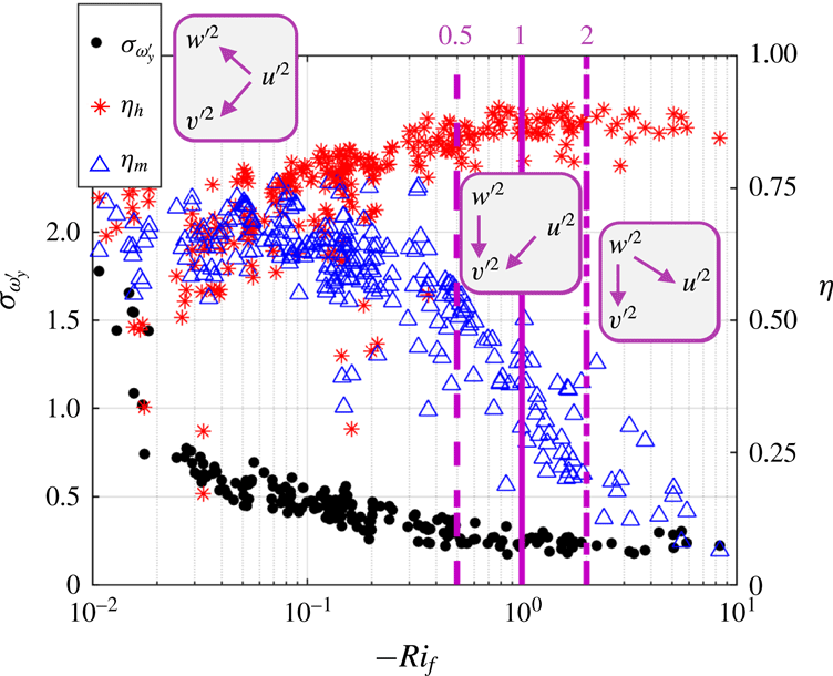
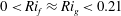
Figure 2. Standard deviation of the perturbation cross-stream vorticity,
 $\unicode[STIX]{x1D70E}_{\unicode[STIX]{x1D714}_{y}^{\prime }}$
, heat transport efficiency,
$\unicode[STIX]{x1D70E}_{\unicode[STIX]{x1D714}_{y}^{\prime }}$
, heat transport efficiency,
 $\unicode[STIX]{x1D702}_{h}$
, and momentum transport efficiency,
$\unicode[STIX]{x1D702}_{h}$
, and momentum transport efficiency,
 $\unicode[STIX]{x1D702}_{m}$
, versus
$\unicode[STIX]{x1D702}_{m}$
, versus
 $Ri_{f}$
. Vertical lines are at
$Ri_{f}$
. Vertical lines are at
 $Ri_{f}=-0.5$
(dashed),
$Ri_{f}=-0.5$
(dashed),
 $-1$
(solid) and
$-1$
(solid) and
 $-2$
(dot-dashed). Experiments and analysis methods are described in Li & Bou-Zeid (Reference Li and Bou-Zeid2011). Purple rectangles depict the directionality of energy transfer.
$-2$
(dot-dashed). Experiments and analysis methods are described in Li & Bou-Zeid (Reference Li and Bou-Zeid2011). Purple rectangles depict the directionality of energy transfer.
(i) At
 $Ri_{f}<-0.5$
,
$Ri_{f}<-0.5$
,
 $R_{w}$
becomes negative, indicating a redistribution out of the vertical component
$R_{w}$
becomes negative, indicating a redistribution out of the vertical component
 $\overline{w^{\prime 2}}$
. The streamwise component, however, remains a source and the cross-stream is now the only net recipient of energy. Furthermore, in the
$\overline{w^{\prime 2}}$
. The streamwise component, however, remains a source and the cross-stream is now the only net recipient of energy. Furthermore, in the
 $\overline{u^{\prime 2}}$
budget, dissipation overtakes redistribution as the main sink. The regime transition indicated by the model at
$\overline{u^{\prime 2}}$
budget, dissipation overtakes redistribution as the main sink. The regime transition indicated by the model at
 $Ri_{f}=-0.5$
can in fact be observed in very high Reynolds number atmospheric flows. One illustration is provided in figure 2, where the standard deviation of the cross-stream perturbation vorticity
$Ri_{f}=-0.5$
can in fact be observed in very high Reynolds number atmospheric flows. One illustration is provided in figure 2, where the standard deviation of the cross-stream perturbation vorticity
 $\unicode[STIX]{x1D70E}_{\unicode[STIX]{x1D714}_{y}^{\prime }}$
(where
$\unicode[STIX]{x1D70E}_{\unicode[STIX]{x1D714}_{y}^{\prime }}$
(where
 $\unicode[STIX]{x1D714}_{y}^{\prime }=\unicode[STIX]{x2202}u^{\prime }/\unicode[STIX]{x2202}z-\unicode[STIX]{x2202}w^{\prime }/\unicode[STIX]{x2202}x$
) and the heat
$\unicode[STIX]{x1D714}_{y}^{\prime }=\unicode[STIX]{x2202}u^{\prime }/\unicode[STIX]{x2202}z-\unicode[STIX]{x2202}w^{\prime }/\unicode[STIX]{x2202}x$
) and the heat
 $\unicode[STIX]{x1D702}_{h}$
and momentum
$\unicode[STIX]{x1D702}_{h}$
and momentum
 $\unicode[STIX]{x1D702}_{m}$
transfer efficiencies measured in the atmosphere above a lake are featured. The efficiencies are defined as the net flux
$\unicode[STIX]{x1D702}_{m}$
transfer efficiencies measured in the atmosphere above a lake are featured. The efficiencies are defined as the net flux
 $F$
of heat or momentum divided by the total downgradient flux from ejections and sweeps
$F$
of heat or momentum divided by the total downgradient flux from ejections and sweeps
 $\unicode[STIX]{x1D702}=F_{total}/F_{downgradient}$
, as detailed in Li & Bou-Zeid (Reference Li and Bou-Zeid2011). At
$\unicode[STIX]{x1D702}=F_{total}/F_{downgradient}$
, as detailed in Li & Bou-Zeid (Reference Li and Bou-Zeid2011). At
 $Ri_{f}\approx -0.5$
, the momentum transfer efficiency begins a rapid decline as the now buoyantly dominated vertical velocity starts to decorrelate from the horizontal component and vertical motions are no longer simply responding to horizontal ones. Furthermore, the decline in
$Ri_{f}\approx -0.5$
, the momentum transfer efficiency begins a rapid decline as the now buoyantly dominated vertical velocity starts to decorrelate from the horizontal component and vertical motions are no longer simply responding to horizontal ones. Furthermore, the decline in
 $\unicode[STIX]{x1D70E}_{\unicode[STIX]{x1D714}_{y}^{\prime }}$
, which encodes information about the structural characteristics of turbulent eddies, and the increase in
$\unicode[STIX]{x1D70E}_{\unicode[STIX]{x1D714}_{y}^{\prime }}$
, which encodes information about the structural characteristics of turbulent eddies, and the increase in
 $\unicode[STIX]{x1D702}_{h}$
slow down. Thus, not only the turbulence energy, but also its structure is modified by buoyancy below this
$\unicode[STIX]{x1D702}_{h}$
slow down. Thus, not only the turbulence energy, but also its structure is modified by buoyancy below this
 $Ri_{f}$
as the vertical component is now dominated by buoyancy generation.
$Ri_{f}$
as the vertical component is now dominated by buoyancy generation.
(ii) At
 $Ri_{f}<-1$
,
$Ri_{f}<-1$
,
 $|R_{w}|>|R_{u}|$
and the
$|R_{w}|>|R_{u}|$
and the
 $w$
component becomes the main supplier of energy in the redistribution interplay but
$w$
component becomes the main supplier of energy in the redistribution interplay but
 $R_{u}$
remains a source as well. The directionality of redistribution (indicated by arrows in figure 2) does not change at this
$R_{u}$
remains a source as well. The directionality of redistribution (indicated by arrows in figure 2) does not change at this
 $Ri_{f}$
. However, turbulence eddy structure and statistics are altered as can be deduced from
$Ri_{f}$
. However, turbulence eddy structure and statistics are altered as can be deduced from
 $\unicode[STIX]{x1D702}_{h}$
, which plateaus beyond this value. This plateau suggests that buoyancy fully dominates the generation of vertical velocity perturbations and their correlation with temperature perturbations, with no effect on heat transport from shear beyond this point.
$\unicode[STIX]{x1D702}_{h}$
, which plateaus beyond this value. This plateau suggests that buoyancy fully dominates the generation of vertical velocity perturbations and their correlation with temperature perturbations, with no effect on heat transport from shear beyond this point.
(iii) At
 $Ri_{f}<-2$
, there is a transition to
$Ri_{f}<-2$
, there is a transition to
 $R_{u}>0$
implying that
$R_{u}>0$
implying that
 $\overline{u^{\prime 2}}$
now becomes a net recipient of energy originating from
$\overline{u^{\prime 2}}$
now becomes a net recipient of energy originating from
 $\overline{w^{\prime 2}}$
. The flow can be considered buoyancy-dominated beyond this point since the streamwise fluctuations are now modulated by buoyantly generated energy. At this value of
$\overline{w^{\prime 2}}$
. The flow can be considered buoyancy-dominated beyond this point since the streamwise fluctuations are now modulated by buoyantly generated energy. At this value of
 $Ri_{f}=-2$
, one can note the onset of a new turbulence regime in figure 2 as
$Ri_{f}=-2$
, one can note the onset of a new turbulence regime in figure 2 as
 $\unicode[STIX]{x1D702}_{m}$
,
$\unicode[STIX]{x1D702}_{m}$
,
 $\unicode[STIX]{x1D702}_{h}$
and
$\unicode[STIX]{x1D702}_{h}$
and
 $\unicode[STIX]{x1D70E}_{\unicode[STIX]{x1D714}_{y}^{\prime }}$
all reach a plateau.
$\unicode[STIX]{x1D70E}_{\unicode[STIX]{x1D714}_{y}^{\prime }}$
all reach a plateau.
On the stable side, as
 $Ri_{f}$
increases from zero:
$Ri_{f}$
increases from zero:
(iv) At
 $Ri_{f}>0.25$
, buoyancy destruction exceeds viscous dissipation in the budget of
$Ri_{f}>0.25$
, buoyancy destruction exceeds viscous dissipation in the budget of
 $\overline{w^{\prime 2}}$
(
$\overline{w^{\prime 2}}$
(
 $\unicode[STIX]{x1D700}_{w}/S<-B/S=Ri_{f}$
), and beyond this point it dominates the damping and the structure of vertical fluctuations.
$\unicode[STIX]{x1D700}_{w}/S<-B/S=Ri_{f}$
), and beyond this point it dominates the damping and the structure of vertical fluctuations.
(v) At
 $Ri_{f}>0.5$
, buoyancy destruction exceeds the total TKE viscous dissipation in all components
$Ri_{f}>0.5$
, buoyancy destruction exceeds the total TKE viscous dissipation in all components
 $\unicode[STIX]{x1D700}$
.
$\unicode[STIX]{x1D700}$
.
(vi) The
 $Ri_{f}=1$
limit is forbidden. The dissipation and the redistribution to the
$Ri_{f}=1$
limit is forbidden. The dissipation and the redistribution to the
 $v$
-component become zero requiring complete laminarization of the flow, while the model predicts
$v$
-component become zero requiring complete laminarization of the flow, while the model predicts
 $R_{u}=R_{w}$
, requiring finite turbulent energy. This point is further examined below to show that a lower limit of
$R_{u}=R_{w}$
, requiring finite turbulent energy. This point is further examined below to show that a lower limit of
 $Ri_{f}\approx 0.21$
exists and that turbulence can be sustained at high stabilities (
$Ri_{f}\approx 0.21$
exists and that turbulence can be sustained at high stabilities (
 $Ri_{g}$
values) provided
$Ri_{g}$
values) provided
 $Re$
remains high.
$Re$
remains high.
4 Extended model with linear Rotta closure
To proceed further in variance modelling, a linear Rotta-type closure for the redistribution term is introduced and is given by
 $$\begin{eqnarray}R_{u}=-\frac{c\unicode[STIX]{x1D700}}{k}\left(\overline{u^{\prime 2}}-\frac{2}{3}k\right)\quad R_{v}=-\frac{c\unicode[STIX]{x1D700}}{k}\left(\overline{v^{\prime 2}}-\frac{2}{3}k\right)\quad R_{w}=-\frac{c\unicode[STIX]{x1D700}}{k}\left(\overline{w^{\prime 2}}-\frac{2}{3}k\right),\end{eqnarray}$$
where
 $k=0.5(\overline{u^{\prime 2}}+\overline{v^{\prime 2}}+\overline{w^{\prime 2}})$
is the TKE and
$k=0.5(\overline{u^{\prime 2}}+\overline{v^{\prime 2}}+\overline{w^{\prime 2}})$
is the TKE and
 $c$
is a model constant. The ratio
$c$
is a model constant. The ratio
 $k/\unicode[STIX]{x1D700}$
represents a characteristic decay time of the turbulence, which here encodes the time required to redistribute variance between components. This model captures the ‘slow’ part of the redistribution and represents the simplest closure one can propose for the return-to-isotropy terms. More detailed models that include the effect of shear and wall blockage, buoyancy and potentially other physical processes, on the pressure–strain correlations have been proposed and used (Canuto et al.
Reference Canuto, Howard, Cheng and Dubovikov2001; Heinze, Mironov & Raasch Reference Heinze, Mironov and Raasch2016). However, to assess the limits of the simplest plausible formulation (and to avoid including other budget equations in the model), we will focus on the linear Rotta closure in this study.
$k/\unicode[STIX]{x1D700}$
represents a characteristic decay time of the turbulence, which here encodes the time required to redistribute variance between components. This model captures the ‘slow’ part of the redistribution and represents the simplest closure one can propose for the return-to-isotropy terms. More detailed models that include the effect of shear and wall blockage, buoyancy and potentially other physical processes, on the pressure–strain correlations have been proposed and used (Canuto et al.
Reference Canuto, Howard, Cheng and Dubovikov2001; Heinze, Mironov & Raasch Reference Heinze, Mironov and Raasch2016). However, to assess the limits of the simplest plausible formulation (and to avoid including other budget equations in the model), we will focus on the linear Rotta closure in this study.
4.1 Model prediction for velocity variances
Inserting the expressions of (4.1) into (2.7)–(2.9), and using
 $S/\unicode[STIX]{x1D700}=(1-Rif)^{-1}$
, yields
$S/\unicode[STIX]{x1D700}=(1-Rif)^{-1}$
, yields
 $$\begin{eqnarray}\displaystyle & \displaystyle \frac{\overline{u^{\prime 2}}}{k}=\frac{S}{c\unicode[STIX]{x1D700}}\left(\frac{2}{3}+\frac{1}{3}Ri_{f}\right)+\frac{2}{3}=\frac{1}{3c}\left(\frac{2+Ri_{f}}{1-Ri_{f}}\right)+\frac{2}{3}, & \displaystyle\end{eqnarray}$$
 $$\begin{eqnarray}\displaystyle & \displaystyle \frac{\overline{v^{\prime 2}}}{k}=\frac{S}{c\unicode[STIX]{x1D700}}\left(-\frac{1}{3}+\frac{1}{3}Ri_{f}\right)+\frac{2}{3}=\frac{1}{3c}\left(\frac{-1+Ri_{f}}{1-Ri_{f}}\right)+\frac{2}{3}=-\frac{1}{3c}+\frac{2}{3}, & \displaystyle\end{eqnarray}$$
 $$\begin{eqnarray}\displaystyle & \displaystyle \frac{\overline{w^{\prime 2}}}{k}=\frac{S}{c\unicode[STIX]{x1D700}}\left(-\frac{1}{3}-\frac{2}{3}Ri_{f}\right)+\frac{2}{3}=\frac{1}{3c}\left(\frac{-1-2Ri_{f}}{1-Ri_{f}}\right)+\frac{2}{3}. & \displaystyle\end{eqnarray}$$
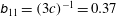
These model variances are shown in figure 3 using
 $c=0.9$
(solid lines), which has been reported as optimal in closure modelling (Pope Reference Pope2000). The
$c=0.9$
(solid lines), which has been reported as optimal in closure modelling (Pope Reference Pope2000). The
 $c=0.9$
(or 1.8 in the full-variance budget) has some theoretical justification (Katul et al.
Reference Katul, Porporato, Manes and Meneveau2013) for neutral flows as well. A notable prediction of the model is that the fraction
$c=0.9$
(or 1.8 in the full-variance budget) has some theoretical justification (Katul et al.
Reference Katul, Porporato, Manes and Meneveau2013) for neutral flows as well. A notable prediction of the model is that the fraction
 $\overline{v^{\prime 2}}/k$
remains independent of stability at a value of approximately 0.3, and this is indeed supported by the LES results (not plotted here) where
$\overline{v^{\prime 2}}/k$
remains independent of stability at a value of approximately 0.3, and this is indeed supported by the LES results (not plotted here) where
 $\overline{v^{\prime 2}}/k\approx 0.25{-}0.35$
at heights
$\overline{v^{\prime 2}}/k\approx 0.25{-}0.35$
at heights
 $z>\unicode[STIX]{x1D6FF}/4$
, where
$z>\unicode[STIX]{x1D6FF}/4$
, where
 $\unicode[STIX]{x1D6FF}$
is the total flow depth. The ratio is higher closer to the wall, but the dependence on stability in the LES runs is weak and non-monotonic.
$\unicode[STIX]{x1D6FF}$
is the total flow depth. The ratio is higher closer to the wall, but the dependence on stability in the LES runs is weak and non-monotonic.

Figure 3. Variance to TKE ratios predicted by the model as a function of
 $Ri_{f}$
: dot–dash lines with
$Ri_{f}$
: dot–dash lines with
 $c=0.7$
, solid lines with
$c=0.7$
, solid lines with
 $c=0.9$
and dashed line with
$c=0.9$
and dashed line with
 $c=1.1$
.
$c=1.1$
.
Under neutral conditions where
 $Ri_{f}=0$
and with
$Ri_{f}=0$
and with
 $c=0.9$
, equations (4.2)–(4.4) yield
$c=0.9$
, equations (4.2)–(4.4) yield
 $\overline{u^{\prime 2}}/k=1.41$
and
$\overline{u^{\prime 2}}/k=1.41$
and
 $\overline{v^{\prime 2}}/k=\overline{w^{\prime 2}}/k=0.3$
, which are reasonably close to values observed in measurements and numerical simulations in the logarithmic region away from the wall (e.g. Bou-Zeid et al. (Reference Bou-Zeid, Meneveau and Parlange2005)), although as discussed before
$\overline{v^{\prime 2}}/k=\overline{w^{\prime 2}}/k=0.3$
, which are reasonably close to values observed in measurements and numerical simulations in the logarithmic region away from the wall (e.g. Bou-Zeid et al. (Reference Bou-Zeid, Meneveau and Parlange2005)), although as discussed before
 $\overline{v^{\prime 2}}/k>\overline{w^{\prime 2}}/k$
. On the other hand, under very strongly unstable conditions when
$\overline{v^{\prime 2}}/k>\overline{w^{\prime 2}}/k$
. On the other hand, under very strongly unstable conditions when
 $-Ri_{f}\gg 1$
and production is dominated by buoyancy,
$-Ri_{f}\gg 1$
and production is dominated by buoyancy,
 $\overline{u^{\prime 2}}$
and
$\overline{u^{\prime 2}}$
and
 $\overline{w^{\prime 2}}$
reverse roles, and
$\overline{w^{\prime 2}}$
reverse roles, and
 $\overline{w^{\prime 2}}/k=1.41$
while
$\overline{w^{\prime 2}}/k=1.41$
while
 $\overline{u^{\prime 2}}/k=\overline{v^{\prime 2}}/k=0.3$
as can be seen in figure 3(a) at the free convection limit of
$\overline{u^{\prime 2}}/k=\overline{v^{\prime 2}}/k=0.3$
as can be seen in figure 3(a) at the free convection limit of
 $Ri_{f}\ll 0$
. The anisotropy of the variance ratios asymptotes to
$Ri_{f}\ll 0$
. The anisotropy of the variance ratios asymptotes to
 $\overline{w^{\prime 2}}/\overline{v^{\prime 2}}\approx \overline{w^{\prime 2}}/\overline{u^{\prime 2}}\approx 4.6$
. These values are close to the
$\overline{w^{\prime 2}}/\overline{v^{\prime 2}}\approx \overline{w^{\prime 2}}/\overline{u^{\prime 2}}\approx 4.6$
. These values are close to the
 ${\approx}3.2$
reported for DNS of free convection above a heated plate by Mellado (Reference Mellado2012), and to the
${\approx}3.2$
reported for DNS of free convection above a heated plate by Mellado (Reference Mellado2012), and to the
 ${\approx}3.4$
of Salesky et al. (Reference Salesky, Chamecki and Bou-Zeid2017) at the lowest
${\approx}3.4$
of Salesky et al. (Reference Salesky, Chamecki and Bou-Zeid2017) at the lowest
 $Ri_{f}$
they studied using LES. The better predictions of the model in the free convection limit, compared to the neutral limit, are not surprising since the energy is being injected in the vertical component and the redistributions to the horizontal components must become equal. This is indicated by the reduced model and the LES in figure 1 and is expected since physically these directions are exactly similar in that limit: the wall effect does not hinder energy redistribution into either horizontal receiving components.
$Ri_{f}$
they studied using LES. The better predictions of the model in the free convection limit, compared to the neutral limit, are not surprising since the energy is being injected in the vertical component and the redistributions to the horizontal components must become equal. This is indicated by the reduced model and the LES in figure 1 and is expected since physically these directions are exactly similar in that limit: the wall effect does not hinder energy redistribution into either horizontal receiving components.
Under stable conditions, a maximum attainable flux Richardson number (
 $Ri_{f,max}$
) emerges beyond which
$Ri_{f,max}$
) emerges beyond which
 $\overline{w^{\prime 2}}<0$
(figure 3
b). This
$\overline{w^{\prime 2}}<0$
(figure 3
b). This
 $Ri_{f,max}$
(
$Ri_{f,max}$
(
 $=$
0.21 for
$=$
0.21 for
 $c=0.9$
) cannot be exceeded because when it is approached,
$c=0.9$
) cannot be exceeded because when it is approached,
 $\overline{w^{\prime 2}}$
approaches zero and buoyancy destruction (
$\overline{w^{\prime 2}}$
approaches zero and buoyancy destruction (
 ${\sim}\overline{w^{\prime }\unicode[STIX]{x1D703}^{\prime }}$
) will be throttled by the rate of redistribution
${\sim}\overline{w^{\prime }\unicode[STIX]{x1D703}^{\prime }}$
) will be throttled by the rate of redistribution
 $R_{w}$
, maintaining
$R_{w}$
, maintaining
 $Ri<Ri_{f,max}$
. That is, the constraint of
$Ri<Ri_{f,max}$
. That is, the constraint of
 $\overline{w^{\prime 2}}>0$
limits the maximum attainable
$\overline{w^{\prime 2}}>0$
limits the maximum attainable
 $R_{w}$
according to (4.1) (it will be the
$R_{w}$
according to (4.1) (it will be the
 $R_{w}$
attained when
$R_{w}$
attained when
 $\overline{w^{\prime 2}}\rightarrow 0$
). This maximum
$\overline{w^{\prime 2}}\rightarrow 0$
). This maximum
 $R_{w}$
then limits the highest attainable energy flux into the vertical component, which must simultaneously limit the buoyant energy destruction in that component (via budget (2.3)). Thus, pressure redistribution of variance from the streamwise to the vertical velocity component becomes the primary regulator of turbulence regime at this asymptotic
$R_{w}$
then limits the highest attainable energy flux into the vertical component, which must simultaneously limit the buoyant energy destruction in that component (via budget (2.3)). Thus, pressure redistribution of variance from the streamwise to the vertical velocity component becomes the primary regulator of turbulence regime at this asymptotic
 $Ri_{f,max}$
. This limiting value of
$Ri_{f,max}$
. This limiting value of
 ${\approx}\,0.21$
is quite consistent with previous estimates (ranging from 0.19 to 0.21) based on second-order moments models that make comparable assumptions to the ones we make here (Yamada Reference Yamada1975; Mellor & Yamada Reference Mellor and Yamada1982), as well as with the asymptotic limit of
${\approx}\,0.21$
is quite consistent with previous estimates (ranging from 0.19 to 0.21) based on second-order moments models that make comparable assumptions to the ones we make here (Yamada Reference Yamada1975; Mellor & Yamada Reference Mellor and Yamada1982), as well as with the asymptotic limit of
 $Ri_{f}$
that can be obtained from its relation to the empirically determined Monin–Obukhov gradient stability correction functions (Wyngaard Reference Wyngaard2010, p. 281). The exact limiting value however might not be 0.21 if buoyancy or other factors (waves, wall-blockage, laminarization, intermittency, non-stationarity, etc.) alter the redistribution efficiency and consequently the value of
$Ri_{f}$
that can be obtained from its relation to the empirically determined Monin–Obukhov gradient stability correction functions (Wyngaard Reference Wyngaard2010, p. 281). The exact limiting value however might not be 0.21 if buoyancy or other factors (waves, wall-blockage, laminarization, intermittency, non-stationarity, etc.) alter the redistribution efficiency and consequently the value of
 $c$
. To account for this possibility and to investigate the change in variances with uncertainties in
$c$
. To account for this possibility and to investigate the change in variances with uncertainties in
 $c$
, figure 3(b) presents the profiles with
$c$
, figure 3(b) presents the profiles with
 $c$
values of 0.7 and 1.1. The attainable
$c$
values of 0.7 and 1.1. The attainable
 $Ri_{f,max}$
limit is reduced to approximately 0.12 for
$Ri_{f,max}$
limit is reduced to approximately 0.12 for
 $c=0.7$
and increased to about 0.28 when
$c=0.7$
and increased to about 0.28 when
 $c=1.1$
. From (4.4), one can derive (again by constraining
$c=1.1$
. From (4.4), one can derive (again by constraining
 $\overline{w^{\prime 2}}$
to remain
$\overline{w^{\prime 2}}$
to remain
 ${>}0$
) the following expression for the dependence on
${>}0$
) the following expression for the dependence on
 $c$
of this asymptotic flux Richardson number as
$c$
of this asymptotic flux Richardson number as
 $Ri_{f,max}=(c-0.5)/(c+1)$
, which increases with increasing
$Ri_{f,max}=(c-0.5)/(c+1)$
, which increases with increasing
 $c$
. That is, the more efficient the redistribution (higher
$c$
. That is, the more efficient the redistribution (higher
 $c$
), the higher the attainable
$c$
), the higher the attainable
 $Ri_{f,max}$
since a high redistribution can sustain a higher buoyancy destruction rate. The limit of
$Ri_{f,max}$
since a high redistribution can sustain a higher buoyancy destruction rate. The limit of
 $Ri_{f,max}\approx 0.25$
, consistent with the classic estimate from linear stability analysis (Miles & Howard Reference Miles and Howard1964) requires
$Ri_{f,max}\approx 0.25$
, consistent with the classic estimate from linear stability analysis (Miles & Howard Reference Miles and Howard1964) requires
 $c=1$
, although we must point out that their result was derived for a bulk
$c=1$
, although we must point out that their result was derived for a bulk
 $Ri$
.
$Ri$
.

Figure 4. Flux versus gradient Richardson numbers from laboratory and atmospheric field experiments, data from Katul et al. (Reference Katul, Porporato, Shah and Bou-Zeid2014).
Atmospheric boundary layer field experiments corroborate the model findings: values of
 $Ri_{f}>\approx 0.21$
are atypical. Gradient and flux Richardson numbers are about equal and vary together between
$Ri_{f}>\approx 0.21$
are atypical. Gradient and flux Richardson numbers are about equal and vary together between
 $0<Ri_{f}\approx Ri_{g}<0.21$
; however, beyond this point,
$0<Ri_{f}\approx Ri_{g}<0.21$
; however, beyond this point,
 $Ri_{f}$
reaches a plateau at
$Ri_{f}$
reaches a plateau at
 $Ri_{f,max}\approx 0.21$
while
$Ri_{f,max}\approx 0.21$
while
 $Ri_{g}$
continues to increase (Katul et al.
Reference Katul, Porporato, Shah and Bou-Zeid2014; van Hooijdonk et al.
Reference van Hooijdonk, Clercx, Ansorge, Moene and van de Wiel2018). This is illustrated in figure 4 where the demarcation between the buoyancy-destruction limited and the redistribution-limited regimes is indicated. Thus, even at higher bulk stabilities, the redistribution throttle mitigates the continuous increase in buoyant destruction and the collapse of turbulence (until the Dougherty–Ozmidov length scale approaches
$Ri_{g}$
continues to increase (Katul et al.
Reference Katul, Porporato, Shah and Bou-Zeid2014; van Hooijdonk et al.
Reference van Hooijdonk, Clercx, Ansorge, Moene and van de Wiel2018). This is illustrated in figure 4 where the demarcation between the buoyancy-destruction limited and the redistribution-limited regimes is indicated. Thus, even at higher bulk stabilities, the redistribution throttle mitigates the continuous increase in buoyant destruction and the collapse of turbulence (until the Dougherty–Ozmidov length scale approaches
 $\unicode[STIX]{x1D702}_{K}$
(Katul et al.
Reference Katul, Porporato, Shah and Bou-Zeid2014)). A further evidence of the physical significance of this
$\unicode[STIX]{x1D702}_{K}$
(Katul et al.
Reference Katul, Porporato, Shah and Bou-Zeid2014)). A further evidence of the physical significance of this
 $Ri_{f}$
limit is that the spectrum of measured vertical velocity above an extensive ice sheet no longer exhibits an inertial subrange when
$Ri_{f}$
limit is that the spectrum of measured vertical velocity above an extensive ice sheet no longer exhibits an inertial subrange when
 $Ri_{f}$
exceeds a threshold estimated at
$Ri_{f}$
exceeds a threshold estimated at
 ${\approx}0.25$
(Grachev et al.
Reference Grachev, Andreas, Fairall, Guest and Persson2013).
${\approx}0.25$
(Grachev et al.
Reference Grachev, Andreas, Fairall, Guest and Persson2013).
Another conclusion that can be drawn from the analysis of the relation between
 $Ri_{f,max}$
and
$Ri_{f,max}$
and
 $c$
is that the value of
$c$
is that the value of
 $c$
must be constrained to
$c$
must be constrained to
 $c>0.5$
(otherwise
$c>0.5$
(otherwise
 $Ri_{f,max}$
in stable flows cannot be
$Ri_{f,max}$
in stable flows cannot be
 ${>}0$
) and
${>}0$
) and
 $c<2.5$
(otherwise
$c<2.5$
(otherwise
 $Ri_{f,max}>1$
). As discussed above,
$Ri_{f,max}>1$
). As discussed above,
 $Ri_{f,max}>1$
cannot be attained when a high-
$Ri_{f,max}>1$
cannot be attained when a high-
 $Re$
flow is stationary, planar–homogeneous and lacking a mean vertical velocity. For the aforementioned conditions,
$Re$
flow is stationary, planar–homogeneous and lacking a mean vertical velocity. For the aforementioned conditions,
 $Ri_{f,max}>1$
results in a negative TKE dissipation rate (i.e. viscous production).
$Ri_{f,max}>1$
results in a negative TKE dissipation rate (i.e. viscous production).
4.2 Model prediction for velocity anisotropy, and the implied Rotta constant
As detailed in the introduction, return to isotropy is a trend, but the turbulence remains anisotropic if production is dominated by one or two components. One important question that emerges is to what degree can return to isotropy succeed in equi-partitioning the energy, and how does buoyancy influence this equi-partitioning. The flow anisotropy is best characterized by the velocity anisotropy tensor
 $$\begin{eqnarray}\unicode[STIX]{x1D623}_{ij}=\frac{{u^{\prime }}_{i}{u^{\prime }}_{j}}{2k}-\frac{\unicode[STIX]{x1D6FF}_{ij}}{3}.\end{eqnarray}$$
Based on (4.2)–(4.4), the diagonal components of this tensor can be modelled as
 $$\begin{eqnarray}\displaystyle & \displaystyle \unicode[STIX]{x1D623}_{11}=\frac{1}{6c}\left(\frac{2+Ri_{f}}{1-Ri_{f}}\right), & \displaystyle\end{eqnarray}$$
 $$\begin{eqnarray}\displaystyle & \displaystyle \unicode[STIX]{x1D623}_{22}=-\frac{1}{6c}, & \displaystyle\end{eqnarray}$$
 $$\begin{eqnarray}\displaystyle & \displaystyle \unicode[STIX]{x1D623}_{33}=\frac{1}{6c}\left(\frac{-1-2Ri_{f}}{1-Ri_{f}}\right), & \displaystyle\end{eqnarray}$$
where the index 1 denotes the streamwise direction, 2 the cross-stream and 3 the vertical. Under neutral conditions and with
 $c=0.9$
, this results in
$c=0.9$
, this results in
 $\unicode[STIX]{x1D623}_{11}=(3c)^{-1}=0.37$
and
$\unicode[STIX]{x1D623}_{11}=(3c)^{-1}=0.37$
and
 $\unicode[STIX]{x1D623}_{22}=\unicode[STIX]{x1D623}_{33}=(-6c)^{-1}=-0.185$
(they sum to zero). These parameters are reported widely in the literature on neutral homogeneous shear flows; they depend on the Reynolds number as well as the shear rate (Pumir Reference Pumir1996; Briard et al.
Reference Briard, Gomez, Mons and Sagaut2016). The values obtained here are within the reported ranges; specifically, at the highest simulated shear rate, Isaza & Collins (Reference Isaza and Collins2009) found
$\unicode[STIX]{x1D623}_{22}=\unicode[STIX]{x1D623}_{33}=(-6c)^{-1}=-0.185$
(they sum to zero). These parameters are reported widely in the literature on neutral homogeneous shear flows; they depend on the Reynolds number as well as the shear rate (Pumir Reference Pumir1996; Briard et al.
Reference Briard, Gomez, Mons and Sagaut2016). The values obtained here are within the reported ranges; specifically, at the highest simulated shear rate, Isaza & Collins (Reference Isaza and Collins2009) found
 $\unicode[STIX]{x1D623}_{11}\approx 0.38$
,
$\unicode[STIX]{x1D623}_{11}\approx 0.38$
,
 $\unicode[STIX]{x1D623}_{22}\approx -0.12$
and
$\unicode[STIX]{x1D623}_{22}\approx -0.12$
and
 $\unicode[STIX]{x1D623}_{33}\approx -0.26$
(notice the 22 and 33 notations in their paper are the inverse of ours). It is to be noted that their simulations were of homogeneous neutral free shear and hence there were no wall or buoyancy; therefore, the asymmetry between the cross-steam and vertical components is due to the effect of shear on the vertical component. The effect of shear is in fact broadly similar to the effect of a wall: it would reduce redistribution to the shear-normal vertical component and result in
$\unicode[STIX]{x1D623}_{33}\approx -0.26$
(notice the 22 and 33 notations in their paper are the inverse of ours). It is to be noted that their simulations were of homogeneous neutral free shear and hence there were no wall or buoyancy; therefore, the asymmetry between the cross-steam and vertical components is due to the effect of shear on the vertical component. The effect of shear is in fact broadly similar to the effect of a wall: it would reduce redistribution to the shear-normal vertical component and result in
 $\unicode[STIX]{x1D623}_{33}<\unicode[STIX]{x1D623}_{22}$
(both negative) or equivalently
$\unicode[STIX]{x1D623}_{33}<\unicode[STIX]{x1D623}_{22}$
(both negative) or equivalently
 $\overline{w^{\prime 2}}<\overline{v^{\prime 2}}$
. That is, the presence of a wall or the influence of shear alter the redistribution and require a modification of the simplest linear Rotta model, and this modification due to shear is in fact often included as the second term in redistribution closure schemes (e.g. Canuto et al.
Reference Canuto, Howard, Cheng and Dubovikov2001).
$\overline{w^{\prime 2}}<\overline{v^{\prime 2}}$
. That is, the presence of a wall or the influence of shear alter the redistribution and require a modification of the simplest linear Rotta model, and this modification due to shear is in fact often included as the second term in redistribution closure schemes (e.g. Canuto et al.
Reference Canuto, Howard, Cheng and Dubovikov2001).
Some studies (Gerz, Schumann & Elghobashi Reference Gerz, Schumann and Elghobashi1989; Holt, Koseff & Ferziger Reference Holt, Koseff and Ferziger1992) also examined
 $\unicode[STIX]{x1D623}_{11}$
,
$\unicode[STIX]{x1D623}_{11}$
,
 $\unicode[STIX]{x1D623}_{22}$
and
$\unicode[STIX]{x1D623}_{22}$
and
 $\unicode[STIX]{x1D623}_{33}$
under non-neutral conditions. The direct measurement from simulations can be compared to predictions of the present model but the influence of buoyancy on redistribution and on the value of the Rotta constant needs to be accounted for example, as in Canuto et al. (Reference Canuto, Howard, Cheng and Dubovikov2001). An alternative approach is in fact to use the present model of the components of the velocity anisotropy tensor (or the variances or variance differences that can also be derived from (4.2) to (4.4)) to estimate the Rotta model constant and how it varies with stability. Such estimates of
$\unicode[STIX]{x1D623}_{33}$
under non-neutral conditions. The direct measurement from simulations can be compared to predictions of the present model but the influence of buoyancy on redistribution and on the value of the Rotta constant needs to be accounted for example, as in Canuto et al. (Reference Canuto, Howard, Cheng and Dubovikov2001). An alternative approach is in fact to use the present model of the components of the velocity anisotropy tensor (or the variances or variance differences that can also be derived from (4.2) to (4.4)) to estimate the Rotta model constant and how it varies with stability. Such estimates of
 $c$
, while possible in principle, proved difficult. They are highly sensitive to the accuracy of the computed or measured variances near
$c$
, while possible in principle, proved difficult. They are highly sensitive to the accuracy of the computed or measured variances near
 $Ri_{f}$
values that would cause the numerators or denominators of (4.6)–(4.8) to approach 0. Computations from DNS for example suggest a reasonable value of
$Ri_{f}$
values that would cause the numerators or denominators of (4.6)–(4.8) to approach 0. Computations from DNS for example suggest a reasonable value of
 $c$
that varies between 0.8 and 1.3, but with no clear trend with increasing stability. As such, while this paper establishes the influence of redistribution of energy on buoyancy modulation of turbulent flows, the influence of buoyancy on redistribution is a topic that requires further investigation.
$c$
that varies between 0.8 and 1.3, but with no clear trend with increasing stability. As such, while this paper establishes the influence of redistribution of energy on buoyancy modulation of turbulent flows, the influence of buoyancy on redistribution is a topic that requires further investigation.
5 Conclusion
A novel perspective on the role energy redistribution plays in wall-bounded flows with buoyancy has been unfolded through a reduced model based on the budgets of the half-variances of the three velocity components. The model makes assumptions that are commonly used in turbulence closure and modelling including stationarity, horizontal homogeneity and production–dissipation equilibrium, hence postulating that vertical energy transport is of secondary importance (though the model can be extended to include transport terms as illustrated in appendix A). The model is hence not applicable near strong density inversions that might exist in geophysical flows. On the other hand, the framework is applicable in the inertial sublayer (logarithmic zone) of wall-bounded flows (between the buffer and outer layers) that extends from a few millimetres to over 100 m in the atmosphere and is therefore of very high relevance. More generally, the model is also applicable, with appropriate modifications, to other similar flows where the assumptions (mainly local TKE production–destruction balance) are satisfied, such as some free shear configurations and flows over inclined heated/cooled walls.
The basic model (2.7)–(2.10) has no tuneable coefficient, while its extended version (4.1)–(4.4) only requires knowledge of the well-studied Rotta constant for the closure of the redistribution terms. Despite this simplicity, the model predictions are far reaching and compare reasonably well with DNS, LES or observational data in terms of energy redistribution variation with
 $Ri_{f}$
, cross-stream velocity-variance independence of stability and the asymptotic anisotropy under free convective conditions. The model also elucidates how the redistribution of energy modulates the influence of stability on the flow. When buoyancy generates turbulence, redistribution controls the transition from a shear-dominated flow at
$Ri_{f}$
, cross-stream velocity-variance independence of stability and the asymptotic anisotropy under free convective conditions. The model also elucidates how the redistribution of energy modulates the influence of stability on the flow. When buoyancy generates turbulence, redistribution controls the transition from a shear-dominated flow at
 $Ri_{f}>\approx -0.5$
(vertical component receives energy from streamwise component), to a buoyancy-dominated regime at
$Ri_{f}>\approx -0.5$
(vertical component receives energy from streamwise component), to a buoyancy-dominated regime at
 $Ri_{f}<\approx -2$
(vertical component dominates and transfers energy to the streamwise component). Under stable conditions, the reduced model yields a realizability constraint of
$Ri_{f}<\approx -2$
(vertical component dominates and transfers energy to the streamwise component). Under stable conditions, the reduced model yields a realizability constraint of
 $Ri_{f,max}\approx 0.21$
. This constraint is related to the limitations on the redistribution of energy from the streamwise to the vertical component that throttle the maximum attainable buoyant destruction to approximately 21 % of shear production. This explains the ‘self-preservation’ of turbulence at large positive gradient Richardson numbers, as well as the origin and magnitude of the much discussed
$Ri_{f,max}\approx 0.21$
. This constraint is related to the limitations on the redistribution of energy from the streamwise to the vertical component that throttle the maximum attainable buoyant destruction to approximately 21 % of shear production. This explains the ‘self-preservation’ of turbulence at large positive gradient Richardson numbers, as well as the origin and magnitude of the much discussed
 $Ri_{f,max}$
. In addition, the linkage in the extended model of the redistribution and the standard Rotta closure offers novel constraints on the Rotta constant
$Ri_{f,max}$
. In addition, the linkage in the extended model of the redistribution and the standard Rotta closure offers novel constraints on the Rotta constant
 $0.5<c<2.5$
. The model hence not only successfully explains some very-broadly observed statistical and structural properties of turbulence at high Reynolds numbers and how they vary with buoyancy, but it also extends the boundaries of our current understanding of the physics and ability to close and simulate turbulent dynamics.
$0.5<c<2.5$
. The model hence not only successfully explains some very-broadly observed statistical and structural properties of turbulence at high Reynolds numbers and how they vary with buoyancy, but it also extends the boundaries of our current understanding of the physics and ability to close and simulate turbulent dynamics.
More broadly, the primary implication of the study is that pressure redistribution, by controlling the communication between the variance components, can explain a significant range of empirically observed turbulent flow dynamics. These return-to-isotropy terms have been much less studied than other terms in the budget equations, partially because they are not yet measurable experimentally, but their physics and relevance warrant more investigations and the model developed here can serve as ‘framework of maximum simplicity’ in these efforts.
Acknowledgements
This work is supported by the Princeton Environmental Institute’s Grand Challenges Program. The authors would also like to thank Professor D. Li for providing the data used in figure 2, as well as the anonymous reviewers for their constructive and thoughtful suggestions. G.G.K. acknowledges partial support from the National Science Foundation (NSF-EAR-1344703, NSF-AGS-1644382, NSF-IOS-1754893, and NSF-DGE-1068871). C.A. acknowledges support through Project C7 of the DFG’s Trans-regional Research Collaborative and a UoC PostDoc Grant.
Appendix A. The potential role of transport
The potential role of transport can be investigated using a modified version of the basic reduced model. If the transport terms denoted by
 $T_{u}$
,
$T_{u}$
,
 $T_{v}$
and
$T_{v}$
and
 $T_{w}$
, which lump the turbulent, pressure and viscous transports, are retained, the half-variance budget equations become (Zilitinkevich Reference Zilitinkevich1973)
$T_{w}$
, which lump the turbulent, pressure and viscous transports, are retained, the half-variance budget equations become (Zilitinkevich Reference Zilitinkevich1973)
 $$\begin{eqnarray}\displaystyle & \displaystyle S+T_{u}+R_{u}-\unicode[STIX]{x1D700}_{u}=0, & \displaystyle\end{eqnarray}$$
 $$\begin{eqnarray}\displaystyle & \displaystyle T_{v}+R_{v}-\unicode[STIX]{x1D700}_{v}=0, & \displaystyle\end{eqnarray}$$
 $$\begin{eqnarray}\displaystyle & \displaystyle B+T_{w}+R_{w}-\unicode[STIX]{x1D700}_{w}=0. & \displaystyle\end{eqnarray}$$
Using the same derivation as in the main text, the model results can be generalized to:
 $$\begin{eqnarray}\displaystyle & \displaystyle \frac{R_{u}}{S}=-\frac{Ri_{f}}{3}-\frac{2}{3}+\frac{1}{3}\frac{T_{w}+T_{v}-2T_{u}}{S}, & \displaystyle\end{eqnarray}$$
 $$\begin{eqnarray}\displaystyle & \displaystyle \frac{R_{v}}{S}=-\frac{Ri_{f}}{3}+\frac{1}{3}+\frac{1}{3}\frac{T_{u}+T_{w}-2T_{v}}{S}, & \displaystyle\end{eqnarray}$$
 $$\begin{eqnarray}\displaystyle & \displaystyle \frac{R_{w}}{S}=\frac{2}{3}Ri_{f}+\frac{1}{3}-\frac{1}{3}\frac{2T_{w}-T_{v}-T_{u}}{S}. & \displaystyle\end{eqnarray}$$
The degree to which these transport terms influence the dynamics depends on whether they partially cancel each other or add up. One can note for example that if they are all equal (with the same sign), the net transport terms in (A 4)–(A 6) will be exactly zero. These transport terms will be more significant under unstable conditions, which might explain the larger discrepancies under such conditions (figure 1) than in stable regimes. Another effect of stability is to increase the effective
 $Re$
, defined as a scale separation between the largest and the dissipative scales, under unstable conditions. This will result in a smaller (larger) Kolmogorov scale under unstable (stable) conditions, resulting in a larger (smaller) number of cascading steps to wipe out anisotropy. Nonetheless, the model compares better to the stable DNS data. These aspects will be further examined in future studies.
$Re$
, defined as a scale separation between the largest and the dissipative scales, under unstable conditions. This will result in a smaller (larger) Kolmogorov scale under unstable (stable) conditions, resulting in a larger (smaller) number of cascading steps to wipe out anisotropy. Nonetheless, the model compares better to the stable DNS data. These aspects will be further examined in future studies.
Appendix B. Description of direct numerical simulations (DNS) of stable flows
The Ekman layer cases are studied by direct numerical simulation (DNS). The set-up and data used here are identical to those in Ansorge & Mellado (Reference Ansorge and Mellado2016), extended by the two more stable cases ri076, ri114 (table 1). Governing flow equations are solved numerically in a non-dimensional framework under the Boussinesq approximation, and boundary conditions correspond to a horizontally periodic Ekman flow over a smooth wall and with a fixed temperature difference between the wall and the free stream. Parameters of this set-up are the geostrophic wind velocity
 $G$
, the fluid kinematic viscosity
$G$
, the fluid kinematic viscosity
 $\unicode[STIX]{x1D708}$
, the Coriolis parameter
$\unicode[STIX]{x1D708}$
, the Coriolis parameter
 $f$
and the buoyancy difference
$f$
and the buoyancy difference
 $B_{0}$
between the wall and free stream. We let
$B_{0}$
between the wall and free stream. We let
 $G$
be the free-stream geostrophic forcing and
$G$
be the free-stream geostrophic forcing and
 $u_{\ast }=\sqrt{\Vert \unicode[STIX]{x1D70F}\Vert /\unicode[STIX]{x1D70C}}$
the friction velocity. For analysis, the coordinate
$u_{\ast }=\sqrt{\Vert \unicode[STIX]{x1D70F}\Vert /\unicode[STIX]{x1D70C}}$
the friction velocity. For analysis, the coordinate
 $x$
is rotated to coincide with the direction of the negative surface shear stress
$x$
is rotated to coincide with the direction of the negative surface shear stress
 $\unicode[STIX]{x1D70F}$
, i.e. the flow is investigated in shear-aligned coordinates in analogy to a channel-flow configuration. The non-dimensional parameters governing the flow set-up are a Reynolds number
$\unicode[STIX]{x1D70F}$
, i.e. the flow is investigated in shear-aligned coordinates in analogy to a channel-flow configuration. The non-dimensional parameters governing the flow set-up are a Reynolds number
 $Re=G^{2}/(f\unicode[STIX]{x1D708})$
that sets the turbulence scale separation of the problem and a bulk Richardson number
$Re=G^{2}/(f\unicode[STIX]{x1D708})$
that sets the turbulence scale separation of the problem and a bulk Richardson number
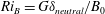 $Ri_{B}=G\unicode[STIX]{x1D6FF}_{neutral}/B_{0}$
describing the stratification in terms of the Buoyancy jump and the boundary layer depth scale under neutral conditions. The turbulent scale separation is given in terms of the boundary layer depth scale in wall units
$Ri_{B}=G\unicode[STIX]{x1D6FF}_{neutral}/B_{0}$
describing the stratification in terms of the Buoyancy jump and the boundary layer depth scale under neutral conditions. The turbulent scale separation is given in terms of the boundary layer depth scale in wall units
 $\unicode[STIX]{x1D6FF}^{+}=u_{\ast }^{2}/(f\unicode[STIX]{x1D708})$
. Times are given as fraction of the inertial period, i.e.
$\unicode[STIX]{x1D6FF}^{+}=u_{\ast }^{2}/(f\unicode[STIX]{x1D708})$
. Times are given as fraction of the inertial period, i.e.
 $t^{-}=tf/2\unicode[STIX]{x03C0}$
and time averaging is denoted by an overbar.
$t^{-}=tf/2\unicode[STIX]{x03C0}$
and time averaging is denoted by an overbar.
A list of DNS cases is given in table 1. The initial condition used for the cases ri014 and ri029 is a realization of the neutrally stratified case ri000, and the buoyancy profile is prescribed by an error function in the wall-normal direction. The stronger stratified cases ri058, ri076 and ri114 use the final states of cases ri014, ri058 and ri076 respectively as initial condition with the buoyancy field adjusted by multiplication with a scalar to match the required
 $Ri_{B}$
. Data are averaged over the period between
$Ri_{B}$
. Data are averaged over the period between
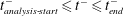 $t_{analysis\text{-}start}^{-}\leqslant t^{-}\leqslant t_{end}^{-}$
(see table 1) to minimize the effect on the analysis of initial adaptations to instantaneous temperature forcing at the bottom (cf. Ansorge & Mellado (Reference Ansorge and Mellado2014)).
$t_{analysis\text{-}start}^{-}\leqslant t^{-}\leqslant t_{end}^{-}$
(see table 1) to minimize the effect on the analysis of initial adaptations to instantaneous temperature forcing at the bottom (cf. Ansorge & Mellado (Reference Ansorge and Mellado2014)).
Table 1. DNS cases for Ekman flow. Grids are
 $2560\times 640\times 5120$
for case
$2560\times 640\times 5120$
for case
 $re_{high}$
and
$re_{high}$
and
 $3072\times 512\times 6144$
for all other cases in streamwise/vertical/cross-stream direction. The streamwise direction of the simulations is rotated by
$3072\times 512\times 6144$
for all other cases in streamwise/vertical/cross-stream direction. The streamwise direction of the simulations is rotated by
 $20.5^{\circ }$
with respect to the geostrophic wind to achieve approximate alignment with the surface stress (for analysis, the data are considered in an exactly shear-stress-aligned coordinate system).
$20.5^{\circ }$
with respect to the geostrophic wind to achieve approximate alignment with the surface stress (for analysis, the data are considered in an exactly shear-stress-aligned coordinate system).

Appendix C. Description of the large eddy simulations (LES) for unstable flows
Table 2. Simulation parameters for the turbulent boundary layers.
 $Ri_{f0}$
is the surface flux Richardson number
$Ri_{f0}$
is the surface flux Richardson number
 $Ri_{f0}=-g/\unicode[STIX]{x1D703}_{0}\langle w^{\prime }\unicode[STIX]{x1D703}^{\prime }\rangle /(\langle u^{\prime }w^{\prime }\rangle \unicode[STIX]{x2202}\langle u\rangle /\unicode[STIX]{x2202}z)$
, where
$Ri_{f0}=-g/\unicode[STIX]{x1D703}_{0}\langle w^{\prime }\unicode[STIX]{x1D703}^{\prime }\rangle /(\langle u^{\prime }w^{\prime }\rangle \unicode[STIX]{x2202}\langle u\rangle /\unicode[STIX]{x2202}z)$
, where
 $g$
is the gravitational acceleration,
$g$
is the gravitational acceleration,
 $\unicode[STIX]{x1D703}$
is temperature and
$\unicode[STIX]{x1D703}$
is temperature and
 $\unicode[STIX]{x1D703}_{0}$
its reference value, angle brackets denote Reynolds averaging and the other variables are as defined in the main text.
$\unicode[STIX]{x1D703}_{0}$
its reference value, angle brackets denote Reynolds averaging and the other variables are as defined in the main text.
 $N_{x,y,z}$
is the number of the grid nodes,
$N_{x,y,z}$
is the number of the grid nodes,
 $z_{i}=800\,\text{m}$
is the height of the inversion base in all unstable simulations,
$z_{i}=800\,\text{m}$
is the height of the inversion base in all unstable simulations,
 $L_{z}$
is the domain height and
$L_{z}$
is the domain height and
 $L$
is the Obukhov length. The non-dimensional time step in all simulations is set to
$L$
is the Obukhov length. The non-dimensional time step in all simulations is set to
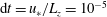 $\text{d}t=u_{\ast }/L_{z}=10^{-5}$
.
$\text{d}t=u_{\ast }/L_{z}=10^{-5}$
.

The details of the LES code are provided in Bou-Zeid, Meneveau & Parlange (Reference Bou-Zeid, Meneveau and Parlange2004), Bou-Zeid et al. (Reference Bou-Zeid, Meneveau and Parlange2005), and for simulations with buoyancy, further details are provided in Huang & Bou-Zeid (Reference Huang and Bou-Zeid2013), Shah & Bou-Zeid (Reference Shah and Bou-Zeid2014b
); and Momen & Bou-Zeid (Reference Momen and Bou-Zeid2017). The code solves the continuity, Navier–Stokes, and heat budget equations for a Boussinesq fluid using a pseudo-spectral method for computing horizontal derivatives and for the test filtering required by the dynamic subgrid-scale (SGS) model. Doubly periodic boundary conditions are hence used in the horizontal directions. A second-order centred difference scheme is used in the vertical direction, requiring a staggered grid. A second-order Adams–Bashforth scheme is used for the time integration. The deviatoric part of the SGS stress tensor is modelled using the scale-dependent Lagrangian dynamic model, where a sharp spectral cutoff filter is used (Bou-Zeid et al.
Reference Bou-Zeid, Meneveau and Parlange2005). Explicit filtering at twice and four times the grid scales is needed for this scale-dependent dynamic approach. At the bottom of the domain (
 $z=0$
), the vertical velocity is set to 0. Since a staggered grid is used, no boundary conditions are needed for the horizontal velocities at the surface. Instead, the stresses associated with vertical fluxes of horizontal momentum are needed; they are modelled through a log-law based equilibrium wall model (Moeng Reference Moeng1984) for the neutral case, with a MOST correction for the unstable or stable cases; a roughness length corresponding to a hydrodynamically rough wall is used in the wall model. Velocities test filtered at twice the grid scale (Bou-Zeid et al.
Reference Bou-Zeid, Meneveau and Parlange2005) are used to obtain an average stress over the wall that is close to the stress obtained from the log law or MOST prediction. In non-neutral simulations conducted for this study, a constant surface heat flux is imposed to produce different static stability conditions. In these simulations, the dimensional surface heat flux
$z=0$
), the vertical velocity is set to 0. Since a staggered grid is used, no boundary conditions are needed for the horizontal velocities at the surface. Instead, the stresses associated with vertical fluxes of horizontal momentum are needed; they are modelled through a log-law based equilibrium wall model (Moeng Reference Moeng1984) for the neutral case, with a MOST correction for the unstable or stable cases; a roughness length corresponding to a hydrodynamically rough wall is used in the wall model. Velocities test filtered at twice the grid scale (Bou-Zeid et al.
Reference Bou-Zeid, Meneveau and Parlange2005) are used to obtain an average stress over the wall that is close to the stress obtained from the log law or MOST prediction. In non-neutral simulations conducted for this study, a constant surface heat flux is imposed to produce different static stability conditions. In these simulations, the dimensional surface heat flux
 $\langle w^{\prime }T^{\prime }\rangle$
varies from 0.0125 to 0.3 (i.e. 0.0125, 0.025, 0.05, 0.1, 0.2, 0.3)
$\langle w^{\prime }T^{\prime }\rangle$
varies from 0.0125 to 0.3 (i.e. 0.0125, 0.025, 0.05, 0.1, 0.2, 0.3)
 $\text{K}~\text{m}\text{s}^{-1}$
, which are typical values observed in field measurements of atmospheric flow over ground surfaces. A stress-free lid condition (i.e. a zero vertical velocity and zero shear stress boundary condition) is imposed at the top of the domain so that the flow corresponds to a half-channel flow with an impermeable centreline (since the Coriolis force is not included). In the unstable cases, the computational domain is larger than the initial boundary layer thickness to enable the atmospheric boundary layer to grow without interacting with the top boundary. In addition, we impose a strong thermal inversion below the top of the computational domain to slow the growth of the boundary layer since with a constant heat flux into the system at the bottom, the boundary layer would keep growing if there are no Coriolis forces. In all of the simulations, the flows are pressure-driven (i.e. forced by a pressure gradient in the streamwise direction), and the pressure gradient balances the surface shear stress under steady-state conditions. The applied pressure forcing hence determines the kinematic wall stress
$\text{K}~\text{m}\text{s}^{-1}$
, which are typical values observed in field measurements of atmospheric flow over ground surfaces. A stress-free lid condition (i.e. a zero vertical velocity and zero shear stress boundary condition) is imposed at the top of the domain so that the flow corresponds to a half-channel flow with an impermeable centreline (since the Coriolis force is not included). In the unstable cases, the computational domain is larger than the initial boundary layer thickness to enable the atmospheric boundary layer to grow without interacting with the top boundary. In addition, we impose a strong thermal inversion below the top of the computational domain to slow the growth of the boundary layer since with a constant heat flux into the system at the bottom, the boundary layer would keep growing if there are no Coriolis forces. In all of the simulations, the flows are pressure-driven (i.e. forced by a pressure gradient in the streamwise direction), and the pressure gradient balances the surface shear stress under steady-state conditions. The applied pressure forcing hence determines the kinematic wall stress
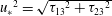 ${u_{\ast }}^{2}=\sqrt{{\unicode[STIX]{x1D70F}_{13}}^{2}+{\unicode[STIX]{x1D70F}_{23}}^{2}}$
, where
${u_{\ast }}^{2}=\sqrt{{\unicode[STIX]{x1D70F}_{13}}^{2}+{\unicode[STIX]{x1D70F}_{23}}^{2}}$
, where
 $\unicode[STIX]{x1D70F}_{13}$
and
$\unicode[STIX]{x1D70F}_{13}$
and
 $\unicode[STIX]{x1D70F}_{23}$
are the stresses at the surface, and the corresponding friction velocity
$\unicode[STIX]{x1D70F}_{23}$
are the stresses at the surface, and the corresponding friction velocity
 $u_{\ast }$
is used to normalize velocities. The length scale we use in normalizations is the nominal boundary layer thickness
$u_{\ast }$
is used to normalize velocities. The length scale we use in normalizations is the nominal boundary layer thickness
 $\unicode[STIX]{x1D6FF}=1000$
m, but the top inversion starts at
$\unicode[STIX]{x1D6FF}=1000$
m, but the top inversion starts at
 $z_{i}=800$
m. A time scale can then be defined using
$z_{i}=800$
m. A time scale can then be defined using
 $\unicode[STIX]{x1D6FF}$
and
$\unicode[STIX]{x1D6FF}$
and
 $u_{\ast }$
; all simulation results are normalized with these scales. The simulation parameters are given in table 2.
$u_{\ast }$
; all simulation results are normalized with these scales. The simulation parameters are given in table 2.