


1. Introduction
With the rising global demand for desalinated ocean water, there is an increasing need to characterize and model the fate and transport of anthropogenic gravity currents caused by the release of brine effluent from coastal desalination plants. Currently, the preferred mode of disposal of the brine from these plants is direct discharge into the ocean, which at present exceeds 120 million cubic metres per day globally (Jones et al. Reference Jones, Qadir, van Vliet, Smakhtin and Kang2019). The salinity of the brine effluent is often 1.6 to 2 times higher than the ambient seawater, resulting in dense gravity currents that have been shown to have adverse impacts on the marine environment (Panagopoulos, Haralambous & Loizidou Reference Panagopoulos, Haralambous and Loizidou2019; Petersen et al. Reference Petersen, Heck, Reguero, Potts, Hovagimian and Paytan2019). The near-coastal environment is also rich in ambient motions, including propagating and breaking internal waves that can mix and alter the vertical structure of the water column at tidal and higher frequencies (Walter et al. Reference Walter, Woodson, Arthur, Fringer and Monismith2012; Sinnett et al. Reference Sinnett, Feddersen, Lucas, Pawlak and Terrill2018). However, the interaction between internal waves and dense gravity currents, and how they may influence one another, has not been the topic of many studies and is not well understood. Prior laboratory experiments by Hogg et al. (Reference Hogg, Egan, Ouellette and Koseff2018) and subsequent numerical simulations by Ouillon et al. (Reference Ouillon, Meiburg, Ouellette and Koseff2019) showed that a single interfacial internal wave colliding with the head of a dense gravity current could reduce the initial downslope net flux by up to 40 %, but no work has been done looking at the longer-term effects on the flux.
More generally, gravity currents are flows, both naturally occurring and anthropogenic, driven by lateral density gradients that play a large role in transporting scalars across a range of environmental settings (Simpson Reference Simpson1997; Baines Reference Baines2008; Cenedese & Adduce Reference Cenedese and Adduce2010; Wells, Cenedese & Caulfield Reference Wells, Cenedese and Caulfield2010). The propagation of a gravity current in a homogeneous ambient environment has been extensively studied in laboratory, computational, theoretical and field settings, leading to well-developed characterizations of the flow (Benjamin Reference Benjamin1968; Britter & Linden Reference Britter and Linden1980; Hallworth et al. Reference Hallworth, Huppert, Phillips and Sparks1996; Cenedese & Adduce Reference Cenedese and Adduce2010; Wells et al. Reference Wells, Cenedese and Caulfield2010; Odier, Chen & Ecke Reference Odier, Chen and Ecke2014; Krug et al. Reference Krug, Holzner, Lüthi, Wolf, Kinzelbach and Tsinober2015; Martin et al. Reference Martin, Negretti, Ungarish and Zemach2020). When the ambient fluid is stratified, the fate and transport of the gravity current becomes more complex, as vertical variations in the density field allow for different levels of neutral buoyancy (Baines Reference Baines2005; Monaghan Reference Monaghan2007). Many researchers have also examined the case of finite-volume lock releases of purely intrusive gravity currents where the gravity current fluid density is bounded by the range of densities of the ambient stratification. These studies have focused on characterizing features such as the frontal speed, velocity structure, instabilities and interfacial disturbances (Holyer & Huppert Reference Holyer and Huppert1980; Britter & Simpson Reference Britter and Simpson1981; Lowe, Linden & Rottman Reference Lowe, Linden and Rottman2002; Flynn & Sutherland Reference Flynn and Sutherland2004; Cheong, Kuenen & Linden Reference Cheong, Kuenen and Linden2006; Maurer & Linden Reference Maurer and Linden2014; Ottolenghi et al. Reference Ottolenghi, Adduce, Roman and La Forgia2020; Wells & Dorrell Reference Wells and Dorrell2021).
The more complex case of a dense gravity current flowing down an incline into a stratified ambient environment where the density of the current exceeds that of all of the ambient has also been the subject of a number of studies focusing on dynamics at both shorter (Monaghan et al. Reference Monaghan, Cas, Kos and Hallworth1999; Baines Reference Baines2005; Samothrakis & Cotel Reference Samothrakis and Cotel2006a,Reference Samothrakis and Cotelb; Baines Reference Baines2008; Cortés, Rueda & Wells Reference Cortés, Rueda and Wells2014; Cortés et al. Reference Cortés, Wells, Fringer, Arthur and Rueda2015) and longer time scales (Rimoldi, Alexander & Morris Reference Rimoldi, Alexander and Morris1996; Wells & Wettlaufer Reference Wells and Wettlaufer2007; Tanimoto, Ouellette & Koseff Reference Tanimoto, Ouellette and Koseff2021). A common feature of these flows is that the gravity current splits at various levels of neutral buoyancy (Monaghan Reference Monaghan2007; Hogg et al. Reference Hogg, Dalziel, Huppert and Imberger2017). In a continuously stratified ambient, multiple levels of neutral buoyancy are available for the gravity current fluid to insert itself as it mixes with the ambient (Baines Reference Baines2005, Reference Baines2008). In a two-layer stratification, which is often more representative of conditions in near-coastal regions, the flow is observed to insert itself at the pycnocline as an interflow or at the bottom of the water column as an underflow (Monaghan et al. Reference Monaghan, Cas, Kos and Hallworth1999; Samothrakis & Cotel Reference Samothrakis and Cotel2006a,Reference Samothrakis and Cotelb; Cortés et al. Reference Cortés, Rueda and Wells2014, Reference Cortés, Wells, Fringer, Arthur and Rueda2015; Tanimoto, Ouellette & Koseff Reference Tanimoto, Ouellette and Koseff2020; Tanimoto et al. Reference Tanimoto, Ouellette and Koseff2021). The interflow, which behaves similarly to an intrusive gravity current despite large differences in the generation mechanism, creates interfacial waves ahead of the gravity current (Monaghan Reference Monaghan2007; Tanimoto et al. Reference Tanimoto, Ouellette and Koseff2020). Furthermore, Rimoldi et al. (Reference Rimoldi, Alexander and Morris1996) and Tanimoto et al. (Reference Tanimoto, Ouellette and Koseff2021) found that in a confined basin, internal waves generated by a gravity current can propagate and reflect, leading to breaking internal waves on the slope at longer times.
The receiving ambient in both natural and engineered systems is often not quiescent, and motion in the ambient has been shown to significantly alter the behaviour of gravity currents (Ellison & Turner Reference Ellison and Turner1959; Fischer & Smith Reference Fischer and Smith1983). Counterflows in the ambient have been shown to arrest and modify the thickness of the gravity current (Britter & Simpson Reference Britter and Simpson1978), and turbulence in the ambient has been shown to alter the gravity current to the point where the propagation of the current is best modelled as a turbulent diffusion process rather than as advection driven by density gradients (Linden & Simpson Reference Linden and Simpson1986). Stratified ambients are also able to support motion in the form of internal waves, and Fischer & Smith (Reference Fischer and Smith1983) found in their field study that internal waves propagating along the thermocline of a lake were responsible for redirecting a portion of an initially negatively buoyant river inflow to the surface.
In the present study we report experimental observations and measurements of a dense gravity current flowing into a two-layered stratified ambient down an incline in the presence and absence of oncoming interfacial internal waves. The experiments reported here differ from those of Hogg et al. (Reference Hogg, Egan, Ouellette and Koseff2018) and Ouillon et al. (Reference Ouillon, Meiburg, Ouellette and Koseff2019) in that there are multiple interfacial internal waves that interact with the body of the gravity current, rather than a transient interaction between a single internal wave and the head of the gravity current. Interfacial internal waves previously investigated by Moore, Koseff & Hult (Reference Moore, Koseff and Hult2016) were chosen, as the boluses formed upon breaking are similar to those observed in the field, for example, by Walter et al. (Reference Walter, Woodson, Arthur, Fringer and Monismith2012) and Sinnett et al. (Reference Sinnett, Feddersen, Lucas, Pawlak and Terrill2018). Our objectives are three-fold: first, to assess whether oncoming internal waves do in fact modify the flux of a gravity current; second, to determine the mechanisms that modify the flux; and third, to assess whether (and how) internal waves affect the ultimate splitting of the gravity current. Details about the experimental methods are presented in § 2, followed by a presentation of the results in § 3 and a discussion and conclusions in § 4.
2. Experimental methods
2.1. Description of the facility
Experiments were carried out in the Stratified Flow Facility in the Bob and Norma Street Environmental Fluid Mechanics Laboratory at Stanford University, as sketched in figure 1. The tank has 25 mm thick acrylic walls and measures 488 cm in length, 30 cm in width and is 61 cm tall. A uniform, rigid, impermeable slope of  $6^{\circ }$ was sealed into the tank. The slope starts at a distance of 85 cm from the downstream end of the tank, extending a horizontal distance of 283 cm such that the top of the slope is at a height of 38.5 cm above the floor of the tank. At the top of the slope, a lock of length 58 cm contained the initial gravity current fluid with a gate to control the release of the current. For other descriptions of the facility, see Troy & Koseff (Reference Troy and Koseff2005), Hult, Troy & Koseff (Reference Hult, Troy and Koseff2009), Moore et al. (Reference Moore, Koseff and Hult2016) and Tanimoto et al. (Reference Tanimoto, Ouellette and Koseff2020, Reference Tanimoto, Ouellette and Koseff2021). Further descriptions of modifications made to the facility for completing the work described in this paper are provided below.

Figure 1. Schematic of the facility and measurement instrumentation. The gravity current is fed from the constant flux tank (a) to the lock above the slope (b). During the experiment the underflow is removed by the main drain (c). The box outlined in blue is the approximate spatial extent of the PLIF–PIV for all experimental runs 1-a to 4-d, and the box outlined in the dashed red is the spatial extent for PLIF–PIV for run 5-a.
The gravity current fluid was supplied from a 225 L tank mounted 2.5 m above the ground and configured as a Mariotte's bottle (labelled ‘(a)’ in figure 1), to function as a constant flow rate apparatus (Maroto, de Dios & de las Nieves Reference Maroto, de Dios and de las Nieves2002). The gravity current supply line was fitted-out with a gate valve for flow control and a ball valve to quickly engage and disengage the outflow. The fluid entered the tank through eight equally spaced diffuser ports spanning the width of the gravity current lock (labelled ‘(b)’ in figure 1) and facing the upstream direction, where a mesh bag filled with horsehair acted to dissipate any momentum associated with the flow, thus focusing the flow in the direction of the slope.
Because our intention was to conduct experiments of longer duration than the typical short releases done previously, we needed to actively control the volume of water in the tank so that the nominal position of the density interface remained constant as the gravity current filled the tank. To do this, the tank was drained at the same volumetric flow rate as the incoming gravity current. For this purpose, the tank is equipped with a drain (labelled ‘(c)’ in figure 1) at the downstream end of the tank. The drainage flow setting is controlled with a gate valve, and the drain can be quickly engaged with a ball valve upstream of this gate valve. Above the drain is a false floor (see figure 1) of length 75 cm located at a height of 13 cm above the tank bottom to guide the most dense fluid into the main drain, thus preventing the current from impinging on the back wall and causing vertical displacement of the density interface and reflections as described in Tanimoto et al. (Reference Tanimoto, Ouellette and Koseff2021). An additional drain, consisting of a vertical funnel connected to a pump, located inside the gravity current lock was used to keep the overall water level constant throughout the experiment. The funnel was centred spanwise in the tank and the plumbing at the base was designed to be symmetric across the width of the tank to keep the gravity current lock laterally homogeneous. The flow rates of both the main drain and gravity current tank were calibrated before the experiment using the installed gate valves. Because the total head at each of the valves was always constant, the flow rates could be controlled in a highly reproducible manner.
Interfacial internal waves were generated by a vertically oscillating half-cylinder of diameter 15 cm mounted on a linear actuator at the downstream end of the tank, similar to the apparatus used by Moore et al. (Reference Moore, Koseff and Hult2016). The linear actuator was operated in a mode where the position of the wave maker is controlled by an analogue voltage generated from a computer.
2.2. Experimental procedure
Prior to each experiment, two 1000 l holding tanks and one 300 l tank were filled with deionized water and allowed to equilibrate to the constant temperature of the room. The stratifying agent used was salt (Cargill Hi-Grade Evaporated Salt), and the saltwater mixture was filtered with a 1  $\mathrm {\mu }$m pleated filter. Depending on the type of experiment, different dyes and solutes were added. For experiments using particle image velocimetry (PIV) and planar laser-induced fluorescence (PLIF), ethanol, Rhodamine 6G and tracer particles were added in addition to the stratifying agent. For flow visualization experiments, green food colouring (McCormick) was added to the lower layer fluid and the gravity current fluid.
The initial conditions for all the experimental runs were the same. A two-layer stratification was established by first filling the tank with the lower layer fluid and then slowly introducing the upper layer fluid via a floating diffuser to minimize mixing between the layers. The initial flow rate for the upper layer was less than 1 l min $^{-1}$ and was gradually increased over time as the upper layer filled. A small amount of salt was added to the upper layer to improve the performance of the conductivity probe in this layer. The upper layer density of
  $\rho _1=1000.27$ kg m
 $^{-3}$ and the lower layer density of
  $\rho _2=1010.94$ kg m
 $^{-3}$, as measured by an Anton Paar 4500 density meter, resulted in a non-dimensional density difference (
 $\rho _2-\rho _1)/\rho _1$ of 1 %. The upper- and lower-layer density and heights were kept constant for all experimental runs at
  $h_1=21$ and
  $h_2=27.5$ cm. A conductivity and thermistor (CT) probe (Precision Measurements Engineering MSCTI model 125) mounted on a linear actuator that traversed vertically downward at a speed of 10 cm s
 $^{-1}$ was used to verify that the ambient stratification was consistent for all the experiments. The thickness of the interface (
 $\delta$) was calculated from the vertical density profiles using the 99 % thickness as defined by Troy & Koseff (Reference Troy and Koseff2005) and Fringer & Street (Reference Fringer and Street2003) as
 \begin{equation} \delta = z\{\rho=0.99(\bar{\rho}-\rho_2\}-z\{\rho=0.99(\rho_1 - \bar{\rho})\}, \end{equation}
where  $\bar {\rho }=(\rho _1 +\rho _2)/2$. The initial interface thickness was
  $\delta =1.3 \pm 0.1$ cm for all the experiments. A slotted pipe described by Troy & Koseff (Reference Troy and Koseff2005) was used to selectively withdraw the intermediate-density fluid to sharpen the interface to this thickness. The initial thickness of the interface of
  $\delta =1.3$ cm is comparable to that of the experiments by Hult et al. (Reference Hult, Troy and Koseff2009) and Moore et al. (Reference Moore, Koseff and Hult2016) investigating the dynamics of breaking interfacial internal waves in the same facility.
Prior to the experiment, the gravity current tank (see figure 1) was filled with the gravity current fluid. The density of the gravity current fluid was kept constant at  $\rho _3=1025.93$ kg m
 $^{-3}$, leading to a non-dimensional density difference of (
 $\rho _3-\rho _1)/\rho _1$ of 2.6 %. Five seconds prior to opening the gate to a height of 3.5 cm, the gravity current inflow and drain within the gravity current tank were engaged. When the dividing gate was lifted, the gravity current flowed down the slope as a constant flux gravity current. Shortly after, the main drain was engaged such that with the inflow of the gravity current and the two drains working in conjunction, the overall water height in the facility was maintained to within 5 mm throughout the experiment. The time when the gate was opened to initiate each experiment is defined to be
  $t=0$ to provide a common time origin for all experiments.
2.3. Quantitative flow imaging
Simultaneous PIV and PLIF using two cameras was used to obtain temporally and spatially resolved measurements of velocity in the horizontal and vertical directions, as well as collocated density measurements. Combined PLIF–PIV is a common technique for calculating fluxes in stratified flow experiments and has been used extensively to study both internal waves and gravity currents (Troy & Koseff Reference Troy and Koseff2005; Hult et al. Reference Hult, Troy and Koseff2009; Odier et al. Reference Odier, Chen and Ecke2014; Dossmann et al. Reference Dossmann, Bourget, Brouzet, Dauxois, Joubaud and Odier2016; Moore et al. Reference Moore, Koseff and Hult2016). Differences in the refractive indices between all fluids were eliminated by using ethanol to increase the refractive index, because fluids of different concentrations of salt will refract the laser path through the water differently. Although some of the procedures in the following sections are not unique to the present experiments, we found that the chemical properties of the solutions differed from what is found in the literature. Therefore, we offer a detailed explanation of the procedures and correction methods, along with constants that can potentially be used by other experimenters, in Appendix A.
The flow was illuminated in an  $x$–
$x$– $z$ plane measuring approximately 0.5 mm thick along the centreline of the tank. The light source was a continuous 532 nm laser (MBP Communications), which was swept across the plane using a scanning mirror (Cambridge Technologies 6200H). Using the sawtooth-like position function derived in Crimaldi & Koseff (Reference Crimaldi and Koseff2001) removed vertical heterogeneities in the light exposure within the light sheet. A dynamic scan is preferred over a cylindrical lens because the resulting laser intensity is uniform across the sheet and avoids distortion (Crimaldi Reference Crimaldi2008). The laser passed through a partially submerged glass plate (see figure 1), which eliminated any distortions of the light sheet due to disturbances at the free surface. Two successive light sheets were produced for each planar measurement realization. The first PIV image was acquired during the first sheet, and the second PIV and PLIF image were acquired with the second sheet. The duration of the light sheet was kept between 8–10 ms and the interval between the end of the first light sheet and beginning of the second light sheet was between 1–5 ms, depending on the flow. This cycle consisting of two successive light sheets was run at 7.5 Hz, resulting in 15 images per second from each camera. The same computer software used to drive the voltage signal to the scanning mirror was also used to send a digital trigger signal to the PIV and PLIF cameras.
2.3.1. PLIF
To measure the density variations in the flow, a fluorescent dye, Rhodamine 6G, was added to each of the three fluids in proportion to the density of that fluid. The Schmidt number of the dye is similar to that of salt, where  $Sc=\nu /\kappa$ (
 $\nu$ is the kinematic viscosity of water and
  $\kappa$ is the molecular diffusivity) is
  $1250$ for Rhodamine 6G and 700 for salt (Crimaldi & Koseff Reference Crimaldi and Koseff2001). Rhodamine 6G is highly resistant to photobleaching, with well known absorption and emission spectra (Larsen & Crimaldi Reference Larsen and Crimaldi2006). The laser is operated at 1 W, well within the weak excitation limit of the dye where there is a linear relationship between the concentration of the dye and the intensity of the emitted light (Crimaldi Reference Crimaldi2008). A CCD camera (Redlake Megaplus ES 4.0/E,
  $2048\times 2048$ pixels, with a Sigma 30 mm F1.4 DC HSM lens) fitted with a bandpass filter to only capture the emitted light from the dye was synchronized to the dynamically scanning mirror. The PLIF images were corrected using the dark response and flat-field imaging techniques of Crimaldi & Koseff (Reference Crimaldi and Koseff2001) along with the two-layer stratification calibration method of Troy & Koseff (Reference Troy and Koseff2005). Although these corrections accounted for heterogeneities in the individual pixels of the camera and the scanning sheet, they did not adjust for attenuation of the laser intensity by the solutes in the flow or by the water itself (Ferrier, Funk & Roberts Reference Ferrier, Funk and Roberts1993; Tian & Roberts Reference Tian and Roberts2003; Crimaldi Reference Crimaldi2008). Following Koochesfahani & Dimotakis (Reference Koochesfahani and Dimotakis1985), the attenuation was corrected in every image assuming that the laser intensity had not been attenuated at the topmost row of the image. The specific attenuation constants are given in Appendix B.
After the corrections and calibrations, a median filter with a kernel size of  $5 \times 5$ pixels was applied to remove the contributions of any particles that may have ‘leaked’ through the bandpass filter. Occasionally, stripes were observed in the images due to inhomogeneities in the light sheet or from air bubbles in the flow; this noise was eliminated without affecting the rest of the image using the stripe filter developed by Münch et al. (Reference Münch, Trtik, Marone and Stampanoni2009).
2.3.2. PIV
To obtain two-dimensional velocity fields, hollow glass microsphere tracer particles (Potters Industries Sphericel 110P8) with a mean particle diameter of 12  $\mathrm {\mu }$m and
  $\rho =1100$ kg m
 $^{-3}$ were added to each of the three fluids. Images of the particle field were captured by a camera (Imperx Bobcat ICL-B2520 CCD camera,
  $2456\times 2058$ pixels, with a SMC Pentax-M 28 mm F2.8 lens) with an optical filter to allow all wavelengths equal to or below that of the laser to pass, thus filtering out the light emitted by the fluorescent dye. The images were preprocessed by removing the global minimum values and using the intensity capping method of Shavit, Lowe & Steinbuck (Reference Shavit, Lowe and Steinbuck2007). The PIV algorithm of Cowen & Monismith (Reference Cowen and Monismith1997) was run in multiple passes with decreasing window sizes, with the smoothed outputs from one pass used as the initial guesses for the subsequent pass. On the last pass, the subpixel cross-correlation peak method of Liao & Cowen (Reference Liao and Cowen2005) was applied. This algorithm has been validated in previous studies, such as in Johnson & Cowen (Reference Johnson and Cowen2018) who made measurements of isotropic turbulence. The final window sizes were
  $32\times 32$ pixels with 75 % overlap, and the resultant vectors were spaced approximately 1.2 mm apart. The output of the PIV was filtered based on the signal-to-noise ratio, calculated as the ratio between the two highest correlation peaks, a local median filter and universal outlier detection filter (Westerweel & Scarano Reference Westerweel and Scarano2005; Charonko & Vlachos Reference Charonko and Vlachos2013). Any gaps in the velocity field were filled using interpolation if more than 50 % of the neighbouring points were present after the filters were applied.
2.4. Non-dimensional framework
We use a Richardson number proposed by Wallace & Sheff (Reference Wallace and Sheff1987) to characterize the gravity current entering the two-layer stratification, given as
 \begin{equation} Ri_{\rho} = \frac{g'_{12}h_1}{B^{2/3}}, \end{equation}
where  $g'_{1j}=g(\rho _j-\rho _1)/\rho _1$ is the reduced gravity for
  $j=2$ (lower layer),
  $j=3$ (gravity current) and
  $B=(g'_{13}Q/b)$ is the buoyancy flux per unit width (here
  $Q$ is the flow rate and
  $b$ is the width of the tank). In the present experiments, only
  $Q$ was varied from 0.08–0.36 l s
 $^{-1}$ so that the gravity current
  $Ri_{\rho }$ ranges from 5.15 to 13.49. The incoming waves are characterized using a wave Froude number defined by Moore et al. (Reference Moore, Koseff and Hult2016) as
 \begin{equation} Fr=\frac{a\omega}{\sqrt{g'_{12}H}}. \end{equation}
Here  $H=h_1 h_2/(h_1 + h_2)$ so that the denominator in (2.3) is the linear long wave speed limit for a Boussinesq two-layer flow;
  $\omega =2 {\rm \pi}/T$ is the frequency of the generated waves, where the period
  $T$ is set at 10 s; and
  $a$ is the amplitude of the waves measured at a location where the bottom of the tank is horizontal, away from the slope. The wave maker forcing frequency
  $\omega$, together with the thicknesses of the ambient layers and their densities, determine the wavenumber
  $k$ according to the two-layer thin-interface dispersion relation (Phillips Reference Phillips1977)
 \begin{equation} \omega^{2} = \frac{gk}{\bar{\rho}} \frac{\rho_2-\rho_1}{\coth{kh_1}+\coth{kh_2}} \end{equation}
resulting in a wavelength  $\lambda =2 {\rm \pi}/k$ of 82 cm for all the experiments. This results in a relative depth kH of 0.9, so that the internal waves cannot be considered as deep water nor shallow water waves. While the dynamics of the breaking characteristics of these internal waves alone (the
  $Ri_\rho =\infty$ case) are outside the scope of the present study, details on the breaking and bolus formation of similar waves are available in Moore et al. (Reference Moore, Koseff and Hult2016).
In the present experiments, only the amplitude  $a$ was varied from 0 to 25 mm, resulting in
  $Fr$ varying from 0 to 0.14. The upper limit of the internal wave
  $Fr$ was not set by the dispersion relation, but rather by the degree of separation that occurs at the wave maker at higher frequencies and amplitudes. The wave maker was tested at
  $T=6.6$ s and the amplitude of the measured waves was no longer a linear function of the amplitude of the wave maker stroke pattern, especially at larger amplitudes. This was not an issue for a wave period of 10 s.
A total of 10 wave periods were generated for each experiment, after which the thickening of the interface adversely affected the formation of the waves and the experiment was terminated. To keep the arrival time of the waves (after the gravity current is initiated) at the slope the same for all experiments, we timed the waves so that the first wave arrived at the intersection of the pycnocline and the slope after the head of the gravity current had penetrated the pycnocline. Similarly, the wave maker was always operated from the same neutral position and only the stroke amplitude was varied between cases, so that the internal waves arrived at the slope consistently at the same phase. The amplitude of the sinusoidal signal to the wave maker was ramped up during the first two wave periods, similar to the operation outlined in Moore et al. (Reference Moore, Koseff and Hult2016). The ramping of the wave maker did not affect the wave frequency, and only the intended frequency of the waves was observed in calibrating the wave maker. Operating the wave maker this way ensured that any differences in the breaking mechanism of the internal waves were not due to variations in the incident phase of the wave as it approached the slope.
We performed a total of 16 different experiments with four different flow rates (and thus  $Ri_{\rho }$ values) and four different internal wave amplitudes (
 $a=0$, 8.3, 12.5 and 25 mm). The full set of parameter values and
  $Ri_{\rho }$ and
  $Fr$ values are listed in table 1. Owing to the slight variations in the density of the fluids for each experiment, the value of
  $Ri_{\rho }$ does vary slightly across an
  $Fr$ set, but much less so compared with the variation across
  $Ri_{\rho }$ sets. Our tagging convention is such that for plots where measurements from the same nominal set of
  $Ri_{\rho }$ conditions are provided, the
  $Ri_{\rho }$ corresponding to the
  $Fr=0$ case is used for reference. For each group of
  $Ri_{\rho }$ conditions, the experiments where
  $Fr>0$ should be compared with the baseline case where
  $Fr=0$. The 16 experiments were performed with the PIV and PLIF cameras located 140 cm downstream of the location where the pycnocline initially intersected with the slope (blue box with solid outline in figure 1). One additional experiment with densities similar to run 1-a (noted as run 5-a in table 1) was performed with the measurement system moved upslope closer to the top of the lower layer (red box with dashed outline in figure 1). Select runs were also repeated with food colouring dye so that the overall progression could be easily visualized and recorded with a 1080p camera.
Table 1. Parameters for the different experimental runs (see text for definitions).

3. Results
The results are presented in three sections. First, we present results from experiments 1-a to 4-d (in § 3.1) describing the qualitative nature of the overall flow development. This serves as a background for the next two sections. Second, we present results (in § 3.2) from run 5-a that illustrate the mechanisms influencing the formation of the gravity current interflow. Because the underflow of the gravity current is not conserved due to the presence of the drain, to examine the observed fluxes we focus purely on the interflow. In § 3.3 to § 3.6, we present detailed analyses focusing on the gravity current and interflow fluxes, as well as the structure of the interflow, for experiments 1-a to 4-d. Finally, in §§ 3.7 and 3.8 we describe how the flux of the gravity current interflow affects other metrics of the interflow.
3.1. Overall flow development
The propagation of a gravity current in a homogeneous ambient, such as occurs in the upper layer in our experiments, has been studied extensively by, among others, Britter & Simpson (Reference Britter and Simpson1978), Britter & Linden (Reference Britter and Linden1980) and Simpson (Reference Simpson1997). The gravity current coming out of the gate quickly adjusts to balance buoyancy flux, entrainment and bottom stress in a constant velocity phase (Britter & Linden Reference Britter and Linden1980). Throughout the propagation in the upper layer, both entrainment of the ambient fluid and detrainment of the gravity current fluid is observed, similar to what was found by, for example, Odier, Chen & Ecke (Reference Odier, Chen and Ecke2012) and Hogg et al. (Reference Hogg, Dalziel, Huppert and Imberger2017).
Consistent with previous observations, when the gravity current reaches the pycnocline, part of it penetrates the pycnocline and continues to propagate along the slope as an underflow, and another part propagates into the pycnocline at a higher level of neutral buoyancy as an interflow (Monaghan et al. Reference Monaghan, Cas, Kos and Hallworth1999; Samothrakis & Cotel Reference Samothrakis and Cotel2006a,Reference Samothrakis and Cotelb; Monaghan Reference Monaghan2007; Cortés et al. Reference Cortés, Rueda and Wells2014, Reference Cortés, Wells, Fringer, Arthur and Rueda2015; Tanimoto et al. Reference Tanimoto, Ouellette and Koseff2020, Reference Tanimoto, Ouellette and Koseff2021). Figure 2 shows the progression in  $20$ second increments beginning at
  $t = 13$ s for run 1-a, the lowest
  $Ri_{\rho }$ case with
  $Fr = 0$ (absence of waves). In figure 2(a) (
 $t =13$ s) the gravity current is seen just reaching the interface. In figure 2(b) (
 $t=33$ s) the pycnocline is raised above the head of the underflow, a phenomenon referred to as a locked wave shown in Tanimoto et al. (Reference Tanimoto, Ouellette and Koseff2020). In figure 2(c) (
 $t=53$ s) the interflow is seen propagating to the left, with the interflow seemingly symmetrically distributed about the original pycnocline location, except for the head which is slightly raised. Also of note when comparing figures 2(a) and 2(b) is the difference in both the horizontal and vertical extents of the lower layer. Initially, the lower layer (dyed in green) extends upslope to the position indicated by the white arrow in figure 2(a), but in the presence of the gravity current the initial shape is deformed and some of the lower layer fluid is displaced above the initial height of the pycnocline (shown as the dotted black line). Some of the lower layer fluid at this point is exiting the system through the main drain; however, the mass lost through the drain does not account for the observed reduction of the extent of the lower layer. The ‘generation’ site of the interflow is shown in figures 2(b) and 2(c) (indicated by the red arrows), where the interflow appears to detach from the gravity current underflow as it inserts itself along the pycnocline. In the last two panels (figure 2d and figure 2e), the interflow and underflow are clearly separate with a region of the ambient lower layer between them, in the region indicated by the green arrows. Although the experiment is designed to minimize reflections, after the locked wave reaches the downstream end of the tank reflections result in a low frequency upstream surge. The surge, which has a wavelength much larger than the wavelength of the oncoming waves, is evident in the slightly concave shape of the interface in figure 2(d). Further evidence of the presence of the surge is the horizontal extent of the lower layer in figure 2(e), which is similar to the initial conditions in figure 2(a), as is the vertical position of the interface. Finally, in figure 2(e) we observe a few higher frequency waves, as was the case in Tanimoto et al. (Reference Tanimoto, Ouellette and Koseff2021).

Figure 2. Snapshots in 20 s intervals for run 1-a starting from  $t=13$ s. The top layer is clear, the bottom layer is dyed green, and the gravity current is dyed blue and descending to the left along the slope. The dotted line is the initial location of the pycnocline. The white arrow in (a) marks the lower layer extending to this location; in (b,c) the red arrows mark the generation site of the interflow; and in (d,e) the green arrows mark where the interflow and underflow are separated by the lower layer fluid.
Figure 3 shows the equivalent development of the interflow but for conditions corresponding to run 1-d, with the lowest  $Ri_{\rho }$ gravity current and the highest
  $Fr$ internal waves. In figure 3(a) (
 $t =12.5$ s) the first oncoming wave is observable spanning across the left support beams where the crest is marked by the red downward arrow. Subsequently, in figure 3(b) the oncoming wave interacts with the locked wave from the head of the gravity current (in the region indicated by the red upward arrow), and the amplitude of the resulting wave is much larger than the amplitude of the oncoming wave in figure 3(a). Starting in figure 3(c), the interflow front starts to exhibit a degree of sinuosity as it propagates along the pycnocline (above the white arrow), which is distorted by the oncoming internal waves. We observe, however, that during this time period the internal waves do not propagate upstream beyond the right-hand support beam. In figures 3(d) and 3(e), the interflow is seen travelling along the interface path set by the internal waves, but there appears to be significantly more interaction with the underflow evident in the areas closer to the interflow generation site, above the areas marked by the white arrows.

Figure 3. Snapshots in 20 s intervals for run 1-d starting at  $t=12.5$ s. See caption for figure 2 for other details. The red arrow in (a) marks the crest of the wave and in (b) the crest of the oncoming and locked wave superimposed. The white arrow in (c) marks where the interflow path is starting to get affected by the internal waves and in (d,e) the interaction between the interflow and underflow is seen in this region.
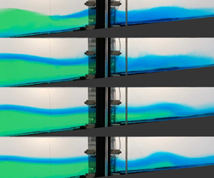
Figure 4 shows side-by-side comparisons of experimental snapshots 30 s apart for runs 4-a (figure 4a–e) and 4-d (figure 4f–j), the runs with the highest  $Ri_{\rho }$ with
  $Fr=0$ and
  $Fr=0.14$, respectively. Compared with figures 2 and 3, the higher
  $Ri_{\rho }$ gravity current does not deform the lower layer as much, and the interflow generation site is much farther upstream, marked by the white arrows in figures 4(b) and 4(g). In figures 4(c) and 4(h) a weak lower-layer surge is observed, returning the pycnocline to its original height. The front for the surge is marked by the white arrows in 4(c) and 4(h), and the re-established pycnocline can be seen in figures 4(d) and 4(i). In the case of the
  $Fr=0.14$ wave, in figure 4(g) the structure of the internal wave is seen upslope of the right-hand support beam, a feature not observed in figure 2 in the lowest
  $Ri_{\rho }$ case. In figures 4(i) and 4(j) the waves (with crests marked by the red arrows) appear to be steepening and forming bolus-like structures similar to those in Moore et al. (Reference Moore, Koseff and Hult2016) but, owing to the much thicker interface from the interflow, the result is perhaps more similar to a turbulent surge rather than a well-defined breaking wave. Comparing the progression in figure 4 with those in figures 2 and 3, it is clear that although the interactions between the internal waves and dense gravity currents have similar qualities, these characteristics depend on the
  $Fr$ of the waves and
  $Ri_{\rho }$ of the gravity current.

Figure 4. Snapshots at 30 s intervals starting at  $t=17$ s, (a–e) are for run 4-a and (f–j) are for run 4-d. The white arrows in (b,g) mark the interflow generation site and in (c,h) the lower layer is returning toward its original position. The red arrows in (i,j) mark the crest of the oncoming internal waves.
3.2. Gravity current profile and interflow generation
Before looking in detail at the results from experiments 1-a to 4-d, we present results from run 5-a that illustrates the mechanism influencing the formation of the gravity current interflow. These experiments utilized a PLIF–PIV system placed along the slope near the top of the lower layer (see location of red box with the dashed outline in figure 1). This specific location was chosen so that simultaneous density and velocity profiles could be acquired both with and without the ambient pycnocline being located upstream of this point. This experiment was performed under the same conditions as run 1-a; the flow development for this case is shown in figure 2. A key observation from figures 2 and 3 is that the lower layer is originally displaced downslope (to the left), allowing the gravity current to flow freely as though it were propagating in a homogeneous ambient. At around  $t=70$ s, the lower layer surges back and the pycnocline (and the top of the lower layer) re-establishes itself upstream of the measurement location.
Collocated temporal measurements of velocity and density in the  $x$–
$x$– $z$ plane were obtained from the combined PLIF–PIV measurements for run 5-a, made in the region where the initial pycnocline and bottom slope intersect (shown as the red box in figure 1). Figure 5 shows the vertical profiles of the density and the horizontal component of the velocity for the gravity current at three different times (
 $t=0$, 22 and 111 s). The profiles are averaged over 2 s to smooth the data and minimize the effect of turbulent fluctuations. The vertical coordinate has been normalized by the height of the gravity current defined by Ellison & Turner (Reference Ellison and Turner1959) as
 \begin{equation} h_u=\frac{\displaystyle\left(\int_0^{\infty} u\,\mathrm{d}z \right)^{2}}{\displaystyle\int_0^{\infty} u^{2} (z)\,\mathrm{d}z}. \end{equation}
Figure 5. Velocity and density profiles of the initial conditions before the experiment ( $t=0$ s), the gravity current in a free-flowing state (
 $t=22$ s) and the gravity current with the pycnocline upstream (
 $t=111$ s). The velocity axis is scaled by the buoyancy flux of the gravity current, and the density by the densities of the ambient stratification. The vertical axis is scaled by the height defined in (3.1). The coordinate system is the same as in figure 1.
The solid line is the initial density profile at  $t=0$ of the ambient layers, which are separated by a thin interface with a hyperbolic tangent shape. The dashed line at
  $t=22$ s in the velocity profile (figure 5a) shows the propagation of the gravity current, which exhibits classic gravity current velocity characteristics with the highest shear at the bottom of the profile (Wells et al. Reference Wells, Cenedese and Caulfield2010; Wells & Dorrell Reference Wells and Dorrell2021). The density profile (figure 5b) at
  $t=22$ s shows the downslope displacement of the lower layer. After the lower layer has re-established itself upstream of this measurement location at
  $t=111$ s, the peak velocity is reduced and the gradient in the velocity profile appears also to be reduced. At
  $t=22$ s the high density of the gravity current is present from
  $z/h_u=0$ to
  $z/h_u = 0.5$ in the density profile, above which is a long tail where the density decreases to the density of the upper layer linearly above
  $z/h_u=0.5$. The density profile at
  $t=111$ s is different from at
  $t=22$ s in that the pycnocline is now upstream of the measurement location at
  $t=111$ s, and it appears that the flow region formerly forming the long tail now consists of fluid of intermediate densities due to mixing of the underflow with the lower ambient fluid. Furthermore, this fluid appears to have been guided into the interflow region of the gravity current, as seen by the increase of the fluid with non-dimensional densities between zero and one in the density profile. This is very similar to the phenomenon known as ‘peeling detrainment’, where partially mixed fluid from the gravity current will selectively separate from the gravity current and seek its own level of neutral buoyancy (Baines Reference Baines2005, Reference Baines2008; Odier et al. Reference Odier, Chen and Ecke2012; Cortés et al. Reference Cortés, Rueda and Wells2014; Hogg et al. Reference Hogg, Dalziel, Huppert and Imberger2017). In the present case, the fluid that is being detrained is ‘guided’ to a region between the two ambient layers, thus forming the gravity current interflow. While the detrained fluid does have some excess horizontal momentum imparted from the underflow, the mixing with the slow-moving ambient fluid that occurs to form the intermediate-density fluid results in the interflow velocity being less than that of the underflow. Although there have been attempts to characterize the velocity of intrusive gravity currents in lock releases (see Cheong et al. (Reference Cheong, Kuenen and Linden2006), for example), there is no unified theory to predict the intrusion velocity of a detraining interflow intrusion forming from a gravity current on a slope, either in stratified environments or in the presence of internal waves.
Because of mixing and entrainment, the density of the detrained fluid is much lower than the density of the original underflow of the fluid. We therefore do not expect the gravity current underflow downstream of the stratified interface ( $t=111$ s in figure 5) to have the same density-profile shape as upstream of that interface (
 $t=22$ s in figure 5). In some previously reported work, the shapes of the velocity and density profiles of the gravity current are found to be similar (or are assumed to be), and integral or bulk measures can be used to characterize the thickness or density of the gravity current using only the velocity profile (Wells et al. Reference Wells, Cenedese and Caulfield2010). However, as is evident here, such approaches may not always be suitable, especially in stratified environments where fluid can detrain and detach from the main gravity current, thus resulting in continually evolving shapes of the density and velocity profiles.
3.3. Fluxes
In this section we examine how the interflow is affected by the presence of oncoming internal waves. Using the velocity and density field measurements from PLIF–PIV for the 16 experiments in runs 1-a to 4-d, we computed the flux through a vertical interrogation plane at the centre of the blue box in figure 1. This location along the slope was chosen so that the upper and lower layer would both be within the imaging extent and the interflow could be thus characterized. We define the interflow as the mass of fluid with a density greater than that of the upper ambient layer and less than that of the lower layer. The mass flux per unit width across this plane can be calculated as
 \begin{equation} \dot{m}(t)=\int_{z_1}^{z_2} u(z,t)\rho(z,t)\,\mathrm{d}z, \end{equation}
where the  $z_1$ and
  $z_2$ are the lower and upper bounds of the interflow, respectively. Both the velocity and density data are averaged horizontally across a length of 1 cm to calculate the flux.
The time series of the cumulative flux of the interflow  $(\int _0^{t} \dot {m}(t')\,\mathrm {d}t')$, or equivalently the total mass per unit width of the interflow that has crossed the interrogation plane, for runs 2a–2d is shown in figure 6. The cumulative fluxes for runs 2-c (
 $Fr=0.09$) and 2-d (
 $Fr=0.14$) with higher
  $Fr$ are reduced following the initial formation of the interflow, as compared with runs 2-a (
 $Fr=0$) and 2-b (
 $Fr=0.05$). The cumulative flux of the
  $Fr=0$ and
  $Fr=0.05$ cases track each other to within the measurement uncertainty, which suggests that the effect of the waves for this
  $Fr$ are minimal. The
  $Fr=0.09$ and
  $Fr=0.14$ cases also have similar fluxes until
  $t=60$ s, when there is a slight reduction in the
  $Fr=0.14$ case. As the formation of the initial interflow occurs before the internal waves arrive at the slope, the effect of the waves appears to be to inhibit the formation of the subsequent interflow, especially at higher
  $Fr$. The reduction in the flux is clearly dependent on
  $Fr$ for this
  $Ri_{\rho }$, although the trends with
  $Fr$ are not gradual, but rather are sharp. The reduction is observed for
  $Fr=0.09$ and
  $Fr=0.14$, but for not
  $Fr=0.05$. It is possible that at some transitional
  $Fr$ between 0.05 and 0.09, the role of the waves changes to reduce the flux.

Figure 6. Cumulative flux per unit width for  $Ri_\rho =6.43$.
The cumulative flux at  $t=150$ s for all 16 experiments (runs 1-a to 4-d) is shown in figure 7. The fluxes are normalized by the cumulative flux for the
  $Fr=0$ case for each corresponding
  $Ri_{\rho }$, which serves as a base case for evaluating the effects of the oncoming internal waves. Across all
  $Ri_{\rho }$, the effect of oncoming waves is to reduce the observed flux of the interflow. However, the complexity of the flows becomes evident when looking at the different wave cases: the degree of reduction in the interflow for each
  $Ri_{\rho }$ is not monotonic with increasing
  $Fr$. For the
  $Ri_\rho =5.15$,
  $6.43$ and
  $8.62$ cases, the effect of increasing
  $Fr$ is to monotonically reduce the cumulative flux, but for the
  $Ri_\rho =13.49$ case there is no trend with increasing
  $Fr$ other than to reduce the flux to approximately 85 % of that of the
  $Fr=0$ case. In the following sections, we evaluate possible causes for the reduced fluxes in the presence of oncoming internal waves.

Figure 7. Cumulative interflow fluxes at  $t=150$ s normalized by the
  $Fr=0$ case for each
  $Ri_{\rho }$.
3.4. Oncoming internal waves
The time series of the displacement for the  $\rho =\bar {\rho }$ isopycnal (as defined in § 2.2 as
  $\bar {\rho }=(\rho _1+\rho _2)/2$) is shown in figure 8 for
  $Ri_\rho =8.62$ (runs from 2-a to 2-d). In the
  ${Fr=0}$ case, in the absence of oncoming waves, both the low frequency surge from
  $t=60$ to 90 s and higher frequency internal waves after
  $t=90$ s can be seen, consistent with what was observed in Tanimoto et al. (Reference Tanimoto, Ouellette and Koseff2021). In the case where
  $Fr>0$, the deflection seen between
  $t=20$ and 30 s is the initial internal wave, which is typically smaller in amplitude compared with the subsequent waves, as the amplitude on the wave maker is ramped up. The peak at around
  $t=35$ s for all cases (including the
  $Fr=0$ case) is the locked wave, or the upward displacement of the isopycnal owing to the passing of the underflow beneath the pycnocline (Tanimoto et al. Reference Tanimoto, Ouellette and Koseff2020). The crest at
  $t=47$ s is the sum of the third internal wave generated, as well as the small-amplitude launched wave generated by the interflow (Tanimoto et al. Reference Tanimoto, Ouellette and Koseff2020). One notable difference between the
  $Fr=0.09$ and
  $Fr=0.14$ cases, beginning with the crest at
  $t=52$ s, is that although the two waves rise in unison, the
  $Fr=0.09$ wave appears to fall faster than the
  $Fr=0.14$ wave. This is a common trend that continues for the following waves, and may be due to the increased mass in the interflow. With the increased mass, the energy in the
  $Fr=0.09$ wave would be insufficient to lift the pycnocline to the maximum wave amplitude as for the
  $Fr=0.14$ case.

Figure 8. Observed displacement of the  $\rho =\bar {\rho }$ isopycnal for
  $Ri_\rho =8.62$.
3.5. Observed velocities and isopycnal displacement
To examine the effects of the internal waves on the dynamics of the interflow, we phase average the flow with the period of the oncoming internal waves. For linear internal waves, the induced velocities in the ambient layers will change sign during a wave period, resulting in times when the induced velocities are aligned with the interflow and times when they are antialigned. Also, as seen in figure 8, the presence of the interflow may affect the waves differently at different phases of the wave, which can be illuminated by phase averaging. The phases of the internal waves are extracted based on the time series of the vertical displacement of the central isopycnal (where  $\rho =\bar {\rho }$) in figure 8. Of the 10 waves generated for each experiment, only wave periods 3–8 were included in the phase averaging, as the first two waves coming off the wave maker were typically smaller in amplitude than the subsequent waves. Furthermore, for the lowest
  $Ri_{\rho }$, by the time the eighth wave is generated, the pycnocline is no longer at its original level and the wave maker is not as effective in generating sinusoidal waves. For all experiments with
  $Fr>0$, the phase (
 $\phi$) across the experiments was found to be very consistent, as the timing of the initiation of the waves and the generation of the gravity current was not altered between experiments.
For the  $Fr=0$ case, because there are no oncoming internal waves, we do not have a wave period that we can use to phase-average the flow. However, given the following considerations, we choose to use the 10 s period of the oncoming waves to perform a phase average in order to compare the flow with the
  $Fr>0$ cases. Figure 8 shows that a gravity current released into a quiescent stratified environment will generate internal motions, the frequencies of which are somewhat constrained by the generation mechanism (namely the perturbation of the pycnocline by the gravity current) and the restoring force of the ambient stratification. Often the motions induced are not limited to a single frequency: the ‘locked’ waves produced by the underflow and the ‘launched’ waves produced by the interflow result in motions of different frequencies (see Tanimoto et al. Reference Tanimoto, Ouellette and Koseff2021). The upper limit of these frequencies is set by what the ambient stratification can support. The challenge when phase averaging using the period of the oncoming internal waves is that in addition to the frequency of the oncoming waves, we are likely to encounter very similar sets of frequencies generated by the gravity current itself. Here we are assuming that these frequencies encountered in the
  $Fr=0$ case also exist in the
  $Fr>0$ experiments and can be linearly superimposed. By averaging the
  $Fr=0$ case in the same way as the
  $Fr>0$ experiments, we are therefore able to compare any differences that may be caused by the oncoming internal waves. We note that we would not expect the phase-averaged quantities in the
  $Fr=0$ case to be independent of phase, because the frequencies of the launched and locked waves are close to the frequency of the oncoming internal waves, and averaging over our limited data set (due to experimental constraints such as thickening of the interface, among others) is not able to remove them completely. If, however, the time record were longer, with sufficient averaging the
  $Fr=0$ case would not vary with phase. With this caveat in mind, the phase-averaged quantities of
  $Fr=0$ provide us with a common basis for comparison between the wave cases for each
  $Ri_{\rho }$.
The phase-averaged vertical profiles of velocity, density and corresponding gradient Richardson number  $Ri_{g}$ obtained with the PLIF–PIV for experiments 1a–d (the lowest
  $Ri_{\rho }$ case) are shown in figure 9. The velocities in figure 9 have been normalized by the overall maximum velocity of the corresponding
  $Fr=0$ case. The density measurements are normalized as
 \begin{equation} \tilde{\rho}(z,\phi)=\frac{\rho(z,\phi)-\rho_1}{\rho_2 - \rho_1} \end{equation}
so that the upper layer has a non-dimensional density of zero and the lower layer a density of one. The gradient Richardson number, defined as
 \begin{equation} Ri_g = \frac{N^{2}}{S^{2}}=\frac{\dfrac{-g}{\rho_1} \dfrac{\partial \rho}{\partial z}}{\left(\dfrac{\partial u}{\partial z} \right)^{2}} \end{equation}
where  $N$ is the Brunt–Väisälä or buoyancy frequency and
  $S$ is the vertical gradient of the horizontal shear, is the ratio of the stabilizing effect of buoyancy to the destabilizing effect of shear in the velocity profiles. Its magnitude serves as an indicator of potential instabilities in the flow that may lead to stirring or irreversible mixing (Peltier & Caulfield Reference Peltier and Caulfield2003).

Figure 9. Phase averaged normalized velocity, density and  $Ri_{g}$ profiles for runs 1-a, 1-b, 1-c and 1-d. The red lines are the vertical location of the maximum velocity and the vertical location of
  $\tilde {\rho }=0.5$, and the dashed lines in the density are the 1 % and 99 % density values. See text for definitions of normalization.
The velocity profiles for all experiments typically show a core region with the highest observed velocities at the centre of the core similar to a jet, with the shear extending into the region above and below the core. For all cases, we found that the difference between the maximum velocity at the core of the interflow and the velocity of the fluid in either of the ambient layers surrounding it is smaller for the top layer than for the bottom layer. The asymmetry is most likely due to the presence of the gravity current underflow which would cause the lower layer fluid between the interflow and underflow to flow upstream faster (to conserve mass), thus increasing the shear between it and the core interflow region. With increasing  $Fr$, we observe differences in the vertical structure in the velocity profile, not only in the vertical location of the interflow core following the sinusoidal pattern induced by the waves but also in the effects of the wave-induced horizontal velocities beneath the crest and above the trough.
For the  $Fr=0.14$ case in figure 9(j–l) we see the most pronounced wave effects appearing as strong asymmetries in the vertical structure of velocities, which are also a strong function of the wave phase. For wave phases between 0 and
  ${\rm \pi}$, and most notably around
  $\phi ={\rm \pi} /2$, there is strong shear underneath the crest of the wave evidenced by closely grouped velocity contours; above the crest of the wave, the velocity contours are spaced farther apart and there is less apparent shear. The same, however, is not true at
  $\phi =3{\rm \pi} /2$, where the shear appears to be more uniformly distributed vertically. This is consistent with the velocity field induced by the internal waves: the vertical profile of the horizontal velocity induced by a mode 1 internal wave is given as
 \begin{equation} u(z,\phi)=a\omega \,\textrm{e}^{\textrm{i}\phi}(\textrm{sech}(lz))^{k/l} \tanh(lz), \end{equation}
where  $l$ is related to the thickness of the density profile (Phillips Reference Phillips1977) and
  $z$ is the vertical coordinate (positive upwards). Beneath the wave crest the induced velocity is negative, leading to strong shear as the interflow and induced velocities have opposite signs. The opposite is true at the wave trough, where the velocities above the pycnocline are negative and those below the pycnocline are positive. While the shape of the velocity profile is clearly a function of phase, the interface thickness based on density does not vary across
  $Fr$, though the sinuosity of the interface position does become stronger (as expected) with increasing
  $Fr$.
$Fr$.
The velocity and density profiles can be combined to create plots of the gradient Richardson number,  $Ri_{g}$, as a function of
  $Fr$, which are also shown in figure 9. These plots also illuminate the changes in the buoyancy and shear balance in the presence of internal waves. The Richardson numbers in these plots are normalized by the critical value of 0.25 for stratified parallel shear flows (Howard Reference Howard1961; Miles Reference Miles1961), and are plotted using a logarithmic scale such that white regions indicate where
  $Ri_{g}$ is critical. In the
  $Fr=0$ case shown in figure 9,
  $Ri_{g}$ often approaches the critical value of 0.25, especially on the lower flank of the interflow. In the core of the velocity structure, higher values of
  $Ri_{g}$ are observed as the core has the strongest density gradients to counteract the destabilizing effects of the shear. Comparing the regions of lower
  $Ri_{g}$ with the velocity and density profiles, it is clear that the lower values of
  $Ri_{g}$ are observed at the edge of the shear envelope (the vertical extent of the shear layer) where the density gradients are the weakest. As
  $Fr$ increases, however, the regions of lower
  $Ri_{g}$ that are susceptible to instabilities shift to lie mainly below the crest, shown by the lighter shades of red. The region of lower values of
  $Ri_{g}$ at the edge of the shear envelope above the interflow is also further reduced for increasing
  $Fr$ (shown by the deeper red colours). This suggests that the effect of the waves could be to stabilize the water column above the interflow by reducing the susceptibility of the flow to instabilities for this
  $Ri_{\rho }$.
These dynamics are largely consistent across flows with increasing  $Ri_{\rho }$, but the effects are most pronounced for
  $Ri_\rho =13.49$ (runs 4a–4b), the flow with the lowest gravity current flow rate. This low flow rate leads to the least amount of momentum imparted to the fluid forming the interflow, and the wave effects are more evident. Figure 10 shows the same set of plots as figure 9, but for the highest
  $Ri_{\rho }$ case of 13.49. The same increased shear under the crest of the wave is observed, and the effect of the internal waves on the velocity is consistent with the lower
  $Ri_{\rho }$ cases. Other general trends in the velocity and density profiles across the wave phases are consistent with the
  $Ri_\rho =5.15$ case, such as the increased wave effects with increasing
  $Fr$, though there are some important differences. Compared with
  $Ri_\rho =5.15$, the vertical extent of the shear envelope looks similar for all phases, but the same is not true for the density. In the
  $Ri_\rho =13.49$ case, the density envelope, the boundaries of which are indicated by the 99 % density contours, is much smaller compared with the
  $Ri_\rho =5.15$ case. The smaller density envelope leads to the simultaneous occurrence of elevated shear and low density gradients throughout the wave phase, resulting in lower values of
  $Ri_{g}$ especially on the upper flank of the velocity profile. While for
  $Ri_\rho =5.15$ the region above the crest for the
  $Fr=0.14$ case was stabilized (with higher values of
  $Ri_{g}$) compared with the
  $Fr=0$ case, in the case of
  $Ri_\rho =13.49$ even the largest waves of
  $Fr=0.14$ cannot stabilize and increase the
  $Ri_{g}$ values above the crest.

Figure 10. Phase averaged normalized velocity, density and  $Ri_{g}$ profiles for runs 4-a, 4-b, 4-c and 4-d. Normalizations and annotations are the same as in figure 9.
3.6. Structure of the velocity and density profile
Here we present more detailed vertical profiles of velocity and density taken in the interflow region to illustrate how the presence of oncoming internal waves reduces the interflow flux. The velocity and density profiles for select wave phases for the  $Ri_\rho =5.15$,
  $Fr=0$ and
  $Fr=0.05$ flow cases are shown in figure 11 (which are snapshots from figure 9). The values have not been made non-dimensional as there is no inherent scaling for the velocity or density of the gravity current interflow. The
  $Fr=0$ case (solid black line) shows the presence of a jet-like velocity with the maximum velocity at the core of the interflow, but with the velocity on each flank reaching different values. The velocity at the bottom flank of the velocity profile is strongly in the upstream direction, whereas the velocity at the top flank is much smaller in magnitude, and generally points downslope. This difference in shear is due to the presence of the underflow of the gravity current along the slope, causing the lower layer to flow in the upstream direction. The velocity profiles for the
  $Fr=0.05$ flow case in figure 11 (dash–dotted red line) show how the vertical position of the velocity maxima in the interflow core is modulated by the oncoming internal waves. In addition, we observe that not only does the position of the peak velocity depend on wave phase but that there is also a reduction in the peak velocity at various wave phases. The density profiles follow a hyperbolic tangent shape, as expected. The density structure is maintained throughout the full wave period but exhibits a vertical shift induced by the sinusoidal pattern of the waves.

Figure 11. Velocity and density profiles for different wave phases for  $Ri_\rho =5.15$,
  $Fr=0$ (solid, black line) and
  $Fr=0.05$ (dash–dot, red line). The velocity and density for the full wave period are shown in figure 9.
To quantify the reduction in velocity, we calculate the average velocity of the interflow and examine how it varies for the different flow cases. To do this we need to define the boundaries of the interflow in the vertical velocity profile. This is done by calculating the height of the interflow on the upper and lower flank of the velocity profile, setting  $z'=0$ as the vertical location where
  $u=\max {(u)}$, and carrying out the integration in either direction using (3.1). As the value of
  $h$ from (3.1) will not converge unless
  $u(|z'|=\infty )=0$,
  $h_u$ is calculated from the velocity profile with the velocity of the ambient layer on the corresponding flank removed such that
 \begin{equation} h_{u,j}=\frac{\displaystyle\left(\int_0^{\infty} u-u_{\infty,j}\,\mathrm{d}z \right)^{2}}{\displaystyle\int_0^{\infty} (u-u_{\infty,j})^{2}\,\mathrm{d}z} \end{equation}
and  $u_{\infty,j}$ is obtained as the average velocity of layer
  $j$, where the density profile shows no significant gradients. The average velocity of the interflow is then given for each phase as
 \begin{equation} \bar{u}(\phi)=\left( h_{u,1}-h_{u,2} \right) ^{{-}1} \int_{h_{u,2}}^{h_{u,1}} u(z',\phi)\,\mathrm{d} z', \end{equation}
where  $h_{u,j}$ refers to the length derived from the velocity profile, the subscript 1 denotes the upper flank of the velocity profile, and the subscript 2 the lower flank. Shown in figure 12 is
  $\bar {u}(\phi )$ for each
  $Ri_{\rho }$ wave flow case divided by
  $\bar {u}(\phi )$ for the
  $Fr=0$ case. Consistent with the reduced interflow fluxes observed in figure 7, we see that
  $\bar {u}(\phi )$ in cases with waves is reduced (normalized velocity value less than unity) compared with the
  $Fr=0$ case for most phases of the waves in all of the flow cases. The one notable exception is the
  $Fr = 0.05$ wave case for the gravity current of
  $Ri_{\rho }$ of 6.43. We checked to see whether these differences in
  $\bar {u}(\phi )$ between the
  $Fr>0$ and
  $Fr=0$ cases were in fact an artefact of the assumption of a simple linear superposition of the interflow velocity field and the wave induced velocity flow. To do this, we scaled the difference in velocities between the
  $Fr>0$ and
  $Fr=0$ case by the corresponding maximum wave-induced velocity,
  $a\omega$. Results were not bounded by values of
  $-1$ and 1, and therefore the reduction in velocity cannot be attributed solely to a linear superposition of the interflow velocity and the wave induced velocity field. For
  $Ri_{\rho }$ of 5.15 and 6.43, the normalized velocity is the smallest at
  $\phi = 0$, and peaks at approximately
  $\phi ={\rm \pi}$. The magnitude of the velocity reduction is also more pronounced than the slight increase in velocity observed at
  $\phi ={\rm \pi}$, such that the velocity is reduced overall. For
  $Ri_\rho =8.62$ and 13.49, the trends in the phase appear to follow the sinusoidal motion of the isopycnals, where a maximum is observed closer to
  $\phi ={\rm \pi} /2$ with a minimum value roughly half a wave period (
 ${\rm \pi}$) later.

Figure 12. Average interflow velocities normalized by the velocity of the  $Fr=0$ case.
3.7. Arclength
For a given  $Ri_{\rho }$, the interface undergoes a set of ever larger amplitude deflections as
  $Fr$ increases, which results in the interflow traversing a longer path to reach the same downstream location. Taking the time series of the vertical displacement of the central isopycnal where
  $\rho =\bar {\rho }$, we quantify the length of this path by calculating the arclength of the isopycnal. The arclength, however, is not a true measure of the distance travelled by a fluid parcel in the interflow, as such a calculation would require a measurement moving with the flow. For each
  $Ri_{\rho }$, the arclength for each case where
  $Fr>0$ (normalized by the arclength for
  $Fr=0$) linearly increases with
  $Fr$. On average across
  $Ri_{\rho }$, the arclengths were 1.3, 1.7 and 2.2 times longer than that of the
  $Fr=0$ case for flows with
  $Fr=0.05$, 0.09 and 0.14, respectively. The uncertainty in the ratios of the arclengths for all cases was
  $\pm$0.1. The increase in arclength in our experiments is driven by the internal waves, which add a vertical oscillation to the path of the interface. The increased arclength, along with the reduced velocities, will reduce the observed fluxes as the interflow travels along a longer path at a slower rate. Such a vertical oscillation will induce a mean vertical velocity (
 $w$) and also horizontal gradients of vertical velocity (
 ${\partial w}/{\partial x}$) and density (
 ${\partial \rho }/{\partial x}$), which could have implications for mixing.
3.8. Change in mass
As the gravity current splits and forms an interflow and underflow, the underflow is removed from the tank via the main drain. However, the mass in the interflow remains in the tank, and by comparing a vertical density profile with the CT probe before and after the experiment, we can assess the change in mass. The ambient upper and lower layers remain intact throughout the experiment (they are not ever fully mixed by the gravity current or internal waves), hence the boundaries between the ambient layers is clear, and by using the density profile we can quantify the change in mass in the pycnocline between the two layers. This change in mass, however, is not a pure measure of the interflow, as fluid of intermediate density can form as the internal waves break, generate turbulence, and lead to irreversible mixing.
Figure 13 shows the ratio of the final-to-initial mass of the interflow for all 16 experiments. The final profile is taken 40 min after the gravity current is released, and the error bars are derived from two successive density profiles taken 5 min apart. The change in mass is consistent for most cases compared with the final cumulative fluxes in figure 7, but the largest differences occur in the  $Fr=0.14$ cases except for in the Ri
 $_\rho =8.62$ case. Whereas the
  $Fr=0.14$ case for each
  $Ri_{\rho }$ typically had the highest reduction in the final cumulative interflow flux compared with the corresponding
  $Fr=0$ case, the change in mass for the
  $Fr=0.14$ case does not show the same reduction (again, with the exception of Ri
 $_\rho =8.62$). There are two possible reasons for this discrepancy. First, the reduced velocity of the
  $Fr>0$ cases along with the increased arclength would lead to the cumulative observed fluxes being lower. Also, as the objective was to assess how internal waves could alter the flux of the gravity current, the integration of the cumulative flux was only carried out while the gravity current was being fed into the tank. Even after the gravity current feed valve is closed, the remaining flow in the apparatus continues to flow out, which would be captured in the final mass. Second, there are motions along the pycnocline after the experiment has ended, which could enhance mixing and lead to an increase in the change in mass, but not the cumulative fluxes. These effects will be most pronounced in the
  $Fr=0.14$ case.

Figure 13. Relative change in the mass of the pycnocline for all experiments from CT probe measurements before and after the experiment.
4. Summary and conclusions
We used laboratory experiments to study the fate of a constant-flux dense gravity current descending a slope into a two-layer stratified environment in the absence and presence of oncoming internal waves. Upon arriving at the density interface, the gravity current split into an interflow that inserted itself along the pycnocline and an underflow that continued to proceed downslope. Using combined measurements of velocity and density from a PLIF–PIV system, we propose a generation mechanism for the interflow, namely that the pycnocline acts as a guide to redirect the path of fluid of certain densities. The cumulative flux of the interflow is reduced in the presence of internal waves for a range of initial gravity current Richardson numbers.
The phase-averaged velocity and density profiles show that lower values of the gradient Richardson number,  $Ri_{g}$, are more commonly observed beneath the wave crest in the first half of the wave period as
  $Fr$ increases. While
  $Ri_{g}$ values themselves are not a measure of the amount of mixing that takes place, they are useful indicators of the likelihood of irreversible mixing. They are also often used in parameterizations of turbulent entrainment and the flux Richardson number. The fact that
  $Ri_{g}$ does vary with the phase and strength of the oncoming waves suggests that although the waves do not directly generate mixing, they can alter the mean flow, which in turn affects the degree of mixing that may occur in the pycnocline region (Ellison & Turner Reference Ellison and Turner1959; Mellor & Yamada Reference Mellor and Yamada1982; Cenedese & Adduce Reference Cenedese and Adduce2010).
The oncoming internal waves reduced the average velocity of the interflow leading to reduced fluxes. The reduction in velocity was observed to vary during the wave period, with reductions being more pronounced during the downward deflection of the interface when its direction of motion is aligned with gravity. The oncoming internal waves also increased the distanced travelled by the interflow by increasing the arclength. The trends in the cumulative fluxes are consistent with the ratio of the final-to-initial mass measured by the CT probe, yet with larger differences pronounced in the  $Fr=0.14$ case.
In the present experiments, the timing difference between the release of the gravity current and the internal waves was kept constant where the first internal wave would arrive at the after the head of the gravity current had passed, so that the gravity current was effectively in steady state. Previous work by Hogg et al. (Reference Hogg, Egan, Ouellette and Koseff2018) and Ouillon et al. (Reference Ouillon, Meiburg, Ouellette and Koseff2019) showed that a single oncoming internal wave interacting with the head of the gravity current can alter the subsequent flow by a process in which a large part of the head of the gravity current is removed, reducing the net downslope flux of the gravity current. The dependence on the timing difference between the gravity current and wave phase remains largely unexplored and a topic for future research.
In concluding, it is helpful to examine our results in the context of field observations of similar phenomena. To do so we use observations of breaking internal waves made by Walter et al. (Reference Walter, Woodson, Arthur, Fringer and Monismith2012) in Monterey Bay, California and Sinnett et al. (Reference Sinnett, Feddersen, Lucas, Pawlak and Terrill2018) in La Jolla, California. For the gravity current we use publicly available information from the Carlsbad Desalination Plant in Southern California, as well as field observations made in the region of the brine discharge from the plant made by Petersen et al. (Reference Petersen, Heck, Reguero, Potts, Hovagimian and Paytan2019). In the present experiments, by developing a quasi-steady state gravity current we are able to examine the interaction of a sequence of 10 internal waves with a gravity current. One way to compare the experiments with the field observations is to look at the ratio of a characteristic time scale of the gravity current to that of the internal waves. A time scale for the gravity current can be derived from the speed of the gravity current (given as  $u_{gc}=1.5B^{1/3}$ by Britter & Linden (Reference Britter and Linden1980)) and the along-slope distance in the upper layer in a two-layer stratification. For the internal waves, a natural time scale is the period of the waves. Observations of breaking internal waves by Walter et al. (Reference Walter, Woodson, Arthur, Fringer and Monismith2012) and by Sinnett et al. (Reference Sinnett, Feddersen, Lucas, Pawlak and Terrill2018) suggest that these events occur at much higher frequencies than the tidal frequency. For the present experiments, the ratio of the gravity current time scale to the internal wave time scale ranges from 1.0 for the
  $Ri_{\rho }=5.15$ case to 1.6 for the
  $Ri_{\rho }=13.49$ case. Field observations at a site nearby by Sinnett et al. (Reference Sinnett, Feddersen, Lucas, Pawlak and Terrill2018) give the depth of the pycnocline as 6 m, and provide the average slope angle. (Sinnett et al. (Reference Sinnett, Feddersen, Lucas, Pawlak and Terrill2018) also observed high frequency internal waves following breaking events at a period of 10 min.) Integrating all this information we find that the ratio of the gravity current time scale to the observed internal wave time scale is approximately 1.7, similar to the value of 1.6 for the
  $Ri_{\rho }=13.49$ case. This suggests that the relative time scales of the gravity current and internal waves of the present study are similar to what is observed in the field observations.
Another consideration to note is the potential effect of the initial thickness of the pycnocline on the splitting dynamics of the gravity current. In the near-coastal environment, the thermocline, or the region where there is variation in the vertical density profile, can occur over 3–4 m as observed by Sinnett et al. (Reference Sinnett, Feddersen, Lucas, Pawlak and Terrill2018). In lake settings, the thermocline has been observed to be as large as 15–20 m as reported by Cotte & Vennemann (Reference Cotte and Vennemann2020). A thicker interface in a two-layer stratification could lead to enhanced detrainment of the gravity current to the interface, as there are more neutral levels of buoyancy. Furthermore, a thicker interface will lower the buoyancy frequency across the ambient two-layer stratification, which would limit the frequency of the internal waves that can be generated by the gravity current. In the extreme case where the interface is infinitely thick, the ambient stratification would resemble a continuous stratification, as investigated by Baines (Reference Baines2005) and Baines (Reference Baines2008). In both cases, detrainment of the gravity current fluid into multiple levels of neutral buoyancy were observed. With the conditions in the field having thicker interfaces, there is a need for further research investigating and quantifying the effects of varying the interface thickness on the dynamics of the propagation of a dense gravity current.
Acknowledgements
The authors thank B. Sabala for the fabrication of the experimental apparatus. The authors also wish to thank the three anonymous reviewers for their helpful comments and suggestions.
Funding
This work was supported by National Science Foundation grant numbers OCE 1634389 and OCE 2022930.
Declaration of interests
The authors report no conflict of interest.
Appendix A. Refractive index matching
When fluids of different densities are present, inhomogeneities in the refractive index can cause errors in both PIV and PLIF (Alahyari & Longmire Reference Alahyari and Longmire1994). To eliminate this problem, a combination of solutes must be used to not only achieve the desired level of stratification but also to allow the fluid to be optically homogeneous. Considerations for choosing combinations of solutes have been explored in detail, including the potential for double diffusion, linearity in the refractive index and density, effects on viscosity and cost (McDougall Reference McDougall1979; Barrett & Van Atta Reference Barrett and Van Atta1991; Daviero, Roberts & Maile Reference Daviero, Roberts and Maile2001; Clément et al. Reference Clément, Guillemain, McCleney and Bardet2018). Furthermore, in experiments with PLIF, the choice of the solutes also needs to reflect the Schmidt numbers of the fluorescent dye and the stratifying agent (Troy & Koseff Reference Troy and Koseff2005). In the present experiments, these considerations were satisfied using salt for the stratifying agent, Rhodamine 6G as the fluorescent dye, and denatured ethanol for the refractive index matching. The use of ethanol to match the refractive index did not damage the tank, and the concentration of ethanol was low enough such that the nonlinear mixing between alcohols and water did not contribute unwanted physics to the flow.
While this combination of solutes is not unique to the present experiments, denatured ethanol includes various additives such that the refractive index and density cannot be obtained simply from tabulations (Daviero et al. Reference Daviero, Roberts and Maile2001). We therefore measured the refractive index and density of both the salt and ethanol (Fisherbrand 90.5 % reagent ethanol) across the relevant concentration range expected in our experiments. The refractive index was measured using a refractometer capable of measuring to within 0.00005.
Figure 14 shows the refractive index and density of salt and ethanol across the range of concentrations used in the experiments. The solvent used was deionized water for both salt and ethanol. We found that, consistent with previous measurements of this type (see Daviero et al. Reference Daviero, Roberts and Maile2001), both the refractive index and density are linear functions of the solute concentration across this range. The refractive index and density are additive for different solutes and take the form
 \begin{equation} \left.\begin{gathered} n=n_0 + \varSigma m c_i, \\ \rho=\rho_0 + \varSigma mc_i, \end{gathered}\right\} \end{equation}
where  $m$ is the slope of the fit of the data in figure 14,
  $n$ is the refractive index,
  $\rho$ is the density,
  $c$ is the concentration (g mass solute per l volume solvent) and
  $i$ is the solute, either ethanol or salt (McDougall Reference McDougall1979). The constants
  $n_0=1.3300$ and
  $\rho _0=0.9980$ g cm
 $^{-3}$ are measured values for the deionized water. The results of the linear regressions are presented in table 2, and show that although both solutes increase the refractive index, increasing the ethanol concentration decreases the density while increasing the salt concentration increases the density. The
  $r^{2}$ scores of the fits were excellent (greater than 0.99), and the 95 % confidence intervals of the slope values were narrow.

Figure 14. Measured refractive index (a) and density (b) of salt and ethanol for refractive index matching. Shading on the plots show the 95 % confidence intervals of the slope fits.
Table 2. Regression results for the refractive index and density of ethanol and salt. Units of  $m$ are refractive index (
 $n$) or density (
 $\rho$) per unit concentration (g l
 $^{-1}$).

The index matching procedure was as follows. First the gravity current fluid was prepared by adding only salt to achieve the target density. As this was the fluid with the highest refractive index, the refractive indices of the other two fluids needed to be matched to this refractive index. The target density was known a priori and held constant for the experiments; thus, for each of the other two fluids the two equations for total refractive index and density were solved simultaneously, where the two free variables were the concentrations of ethanol and salt in each. Additional considerations on different pairs of chemicals for refractive index matching are summarized well by Clément et al. (Reference Clément, Guillemain, McCleney and Bardet2018).
Appendix B. PLIF correction constants
The attenuation of the laser power along a beam path is described by the Beer–Lambert law so that
 \begin{equation} P=P_0 \exp({\eta(s-s_0)}), \end{equation}
where  $P$ is the power at a location
  $s$,
$s$,  $P_0$ is the power at a location
  $s_0$ and
  $\eta$ is the total attenuation coefficient (Ferrier et al. Reference Ferrier, Funk and Roberts1993). The attenuation coefficient can be calculated in a very similar way to the refractive index and density, and takes the form
 \begin{equation} \eta=\eta_0 + \varSigma m c_i, \end{equation}
where the individual sources of attenuation are additive, and  $\eta _0$ is the clear water attenuation for deionized water, which we take to be 0.00028 cm
 $^{-1}$ (Hass & Davisson Reference Hass and Davisson1977). In the present case, the water, salt, ethanol and Rhodamine 6G dye are all sources of attenuation and must be accounted for. While Daviero et al. (Reference Daviero, Roberts and Maile2001) provide values for these solutes, they are not helpful here because of the differences in ethanol sources. Hence, we measured the attenuation using a laser power meter (Ophir Nova II) for a range of concentrations of all the solutes.
Figure 15 shows the fit of (B1) to the calibration data for the different solutes, and the attenuation constants are provided in table 3. The units for the concentration of salt are g solute l $^{-1}$ solvent, and
  $\mathrm {\mu }$g l
 $^{-1}$ for Rhodamine 6G. The
  $r^{2}$ value for ethanol is somewhat lower than for the other two solutes, but as shown in figure 15 the attenuation for the ethanol is an order of magnitude lower than that for salt and so its contribution is negligible. Our finding is in contrast to the attenuation values shown in Daviero et al. (Reference Daviero, Roberts and Maile2001) where the constants for ethanol were of the same order of magnitude as for Rhodamine and salt. If we had used the corrective procedures of Koochesfahani & Dimotakis (Reference Koochesfahani and Dimotakis1985) with these values, we would have obtained erroneously high values of concentration in the present study. The differences may be attributed to the additives and the type of ethanol used, but it is good practice to follow a similar procedure to quantify the attenuation constants rather than to simply use previously documented values.

Figure 15. Measured laser power attenuation for different solvents. Shading on the plots show the 95 % confidence intervals of the slope fits.
Table 3. Regression results for the attenuation coefficients of ethanol, salt and Rhodamine 6G. Units of  $m$ are cm
 $^{-1}$(g l
 $^{-1}$)
 $^{-1}$.


