


1. Introduction
Many flows occurring in marine, coastal and estuarine environments result from the superposition of surface waves and currents, the latter often driven by either tidal forcing or other long-range hydraulic head differences. Turbulence features that emerge from the wave–current interaction (WCI) influence a variety of environmentally and ecologically relevant processes such as sediment transport (e.g. Madsen & Grant Reference Madsen and Grant1976; Dyer & Soulsby Reference Dyer and Soulsby1988; Blondeaux Reference Blondeaux2001; Green & Coco Reference Green and Coco2014; Fagherazzi et al. Reference Fagherazzi, Edmonds, Nardin, Leonardi, Canestrelli, Falcini, Jerolmack, Mariotti, Rowland and Slingerland2015), microbiota dynamics (Guasto, Rusconi & Stocker Reference Guasto, Rusconi and Stocker2012), transport of nutrients and contaminants (De Souza Machado et al. Reference De Souza Machado, Spencer, Kloas, Toffolon and Zarfl2016) and evolution of saltmarshes (Fagherazzi et al. Reference Fagherazzi2012; Francalanci et al. Reference Francalanci, Bendoni, Rinaldi and Solari2013). For what concerns engineering applications, wave–current turbulence plays a key role in dictating the power output, the mechanical loads and wake dynamics of hydrokinetic marine turbines (Gaurier et al. Reference Gaurier, Davies, Deuff and Germain2013; De Jesus Henriques et al. Reference De Jesus Henriques, Tedds, Botsari, Najafian, Hedges, Sutcliffe, Owen and Poole2014; Noble et al. Reference Noble, Draycott, Nambiar, Sellar, Steynor and Kiprakis2020), and the scour around marine and coastal structures (Sumer et al. Reference Sumer, Petersen, Locatelli, Fredsøe, Musumeci and Foti2013; Sumer Reference Sumer2014).
While its relevance is not in dispute, the study of turbulence in wave–current flows is still in its infancy. The majority of existing experimental works focus on the analysis of mean velocity and shear stress profiles, due to their importance for the modelling of sediment transport (Soulsby et al. Reference Soulsby, Hamm, Klopman, Myrhaug, Simons and Thomas1993). Only sporadically, the attention has turned to investigating the structure of turbulence, in a broader sense, which results from the interaction between currents and either opposed (e.g. Kemp & Simons Reference Kemp and Simons1983; Klopman Reference Klopman1994; Umeyama Reference Umeyama2005, Reference Umeyama2009b; Yuan & Madsen Reference Yuan and Madsen2015; Roy, Samantaray & Debnath Reference Roy, Samantaray and Debnath2018) or following waves (e.g. Van Hoften & Karaki Reference Van Hoften and Karaki1976; Kemp & Simons Reference Kemp and Simons1982; Klopman Reference Klopman1994; Umeyama Reference Umeyama2005, Reference Umeyama2009b; Carstensen, Sumer & Fredsøe Reference Carstensen, Sumer and Fredsøe2010; Yuan & Madsen Reference Yuan and Madsen2015; Singh & Debnath Reference Singh and Debnath2016; Roy, Debnath & Mazumder Reference Roy, Debnath and Mazumder2017; Zhang & Simons Reference Zhang and Simons2019). All these studies agree on the fact that the WCI is strongly nonlinear, namely that the mean flow properties of the combined flow does not match those resulting from the linear superimposition of the current-alone (CA) and wave-alone (WA) flows. For example, compared with CA flows, combined flows in which waves follow a current display mean velocities higher near the bed and lower in the upper part of the water column, and dampened Reynolds stresses (e.g. Umeyama Reference Umeyama2005, Reference Umeyama2009b; Singh & Debnath Reference Singh and Debnath2016).
However, there is no clear understanding of how and why different velocity statistics respond to different combinations of waves and currents. Most experimental results are presented dimensionally because there is no general agreement on the correct scaling that should be employed to compare velocity statistics as measured in different flow conditions. Further, the characterization of turbulence in terms of dominant eddies (i.e. the eddies bearing the largest contribution to different turbulent kinetic energy components) resulting from the nonlinear interaction between waves and currents remains largely unexplored. This knowledge-gap represents a bottleneck for the development of appropriate and physically based modelling strategies and it is not surprising that past attempts to model combined wave–current (WC) flows obtained fair but limited success (see e.g. Grant & Madsen Reference Grant and Madsen1979; Myrhaug Reference Myrhaug1984; Davies, Soulsby & King Reference Davies, Soulsby and King1988; Huang & Mei Reference Huang and Mei2003; Olabarrieta, Medina & Castanedo Reference Olabarrieta, Medina and Castanedo2010; Tambroni, Blondeaux & Vittori Reference Tambroni, Blondeaux and Vittori2015).
Much of the literature devoted to the study of WC flows at a fundamental level relates to experimental studies carried out in laboratory settings. The commonly employed approach involves exploring how the mean and turbulence flow properties of a CA flow (i.e. the benchmark flow) are altered by the passage of waves with different frequency and amplitude. In this respect, the present paper is no different. However, with respect to past studies, it overcomes some experimental shortcomings that are now presented and discussed to highlight some of the novelties introduced herein.
Most previous laboratory studies were carried out by establishing flows with aspect ratios (i.e. the ratio between the channel width and the flow depth) lower than five, a value that Nezu & Nakagawa (Reference Nezu and Nakagawa1993) indicated as the threshold below which lateral walls affect turbulent properties in the mid cross-section of CA flows. For WC flows, such lateral-wall effects have never been systematically investigated and are largely unknown hence, when comparing WC with CA flows, low aspect ratios make it difficult to discern whether the observed differences in turbulence properties are due to effects from the lateral walls or waves.
The aspect ratio is also known to significantly affect the scaling of energetic large eddies populating CA flows (often referred to as very-large scale motions, VLSMs, see Peruzzi et al. Reference Peruzzi, Poggi, Ridolfi and Manes2020; Zampiron, Cameron & Nikora Reference Zampiron, Cameron and Nikora2020). In an attempt to shed light on the size and scaling of dominant eddies emerging from the interaction between waves and currents, this is an issue that should be taken into account when interpreting experimental data but, so far, it has been ignored probably because the interlinks between VLSMs and aspect ratio in open-channel flows have been identified only very recently.
Another shortcoming of past studies relates to the fact that benchmark flows (i.e. CA) were never established with boundary layers covering the entire water column. This, in addition to not being representative of flow conditions normally encountered in the field (Sellar et al. Reference Sellar, Wakelam, Sutherland, Ingram and Venugopal2018), implies that waves were superimposed to ‘hybrid’ shear flows displaying boundary layer properties up to some elevations from the bed and not well-defined (and difficult to replicate) features further above where, presumably, residual inlet turbulence persists. Such residual turbulence is facility-dependent and hence prevents experimental data from displaying flow features of general validity.
To advance the comprehension of turbulence in WC flows, the present study reports results obtained from novel experiments involving waves that follow a steady current generated in a laboratory smooth-bed open-channel flume. Turbulence statistics obtained from an unperturbed open-channel flow were used as a benchmark to study the alterations caused by the passage of waves in WC flows involving a range of wave amplitudes and frequencies. The water surface level was monitored using five ultrasonic gauges positioned along the flume and the two-dimensional (2-D) flow velocity field was measured using a laser Doppler anemometer (LDA). Much of the aforementioned experimental limitations are here overcome because: (i) the aspect ratio was kept above five to minimise lateral walls effects on turbulence statistics in the centreline of the flume where the measurements were collected; (ii) the benchmark (i.e. CA) experiment displayed a boundary layer thickness coinciding with the water depth and well-defined turbulence properties as per self-similar turbulent open-channel flows over smooth beds; and (iii) VLSM properties in the benchmark experiment were well documented and classified.
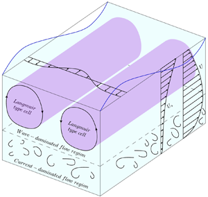
The experimental procedure and the employed laboratory equipment used to carry out the experiments are described in § 2. Section 3 is then dedicated to the description of the signal-decomposition technique (empirical mode decomposition, EMD) that was employed to extract the turbulent signal from velocity measurements and hence to compute some of the velocity statistics used to interpret turbulence in WC flows. In § 4 results are presented and discussed starting from the analysis of mean velocity profiles (§ 4.1) where we identify a novel length scale  $h_0$, which we prove to be key for the analysis and interpretation of turbulence in combined flows. This was explored through the analysis of second-order moments of turbulent velocity fluctuations (§ 4.2) and spectral analysis (§§ 4.3 and 4.4). The latter was successfully employed to investigate the fate of VLSMs in combined flows as well as to identify, for the first time, other large-scale structures that we speculate as being induced by wave motion in ways that are somewhat similar to those responsible for the generation of Langmuir turbulence in ocean flows. In § 5 we discuss the mechanisms generating the Langmuir-type cells, and in § 6 we summarise the main results of the present paper.
2. Methodology
2.1. Equipment
The experiments were carried out in the same flume facility and with the same set-up and instrumentation as those described by Peruzzi et al. (Reference Peruzzi, Poggi, Ridolfi and Manes2020). For this reason, in the text that follows we provide only a brief description of the equipment; for further details we encourage the reader to refer to the paper by Peruzzi et al. (Reference Peruzzi, Poggi, Ridolfi and Manes2020).
The experiments were conducted in a non-tilting, recirculating open-channel flume at the Giorgio Bidone Hydraulics Laboratory of Politecnico di Torino (figure 1a). The flume had glass sidewalls and was 50 m long with a rectangular cross-section that was 0.61 m wide and 1 m deep. To allow for near-wall LDA measurements (described below), the flume bottom was raised with smooth concrete blocks over the original bed. Close to the inlet section, the original bed and the concrete blocks were gently connected by a stainless-steel ramp (figure 1b,c), which was designed to prevent boundary layer separation (Bell & Mehta Reference Bell and Mehta1988) and hence the shedding of undesirable large-scale eddies in the developing flow. To reduce the incoming turbulence generated by the hydraulic circuit, a series of wire fine-mesh screens were located in the sump underlying the flume inlet (figure 1b). For all the experiments, the test section was located at  $x=30$ m (the longitudinal, vertical and spanwise coordinates are indicated with
  $x$,
$x$,  $y$ and
  $z$, respectively, and defined as indicated in figure 1d) from the origin (see figure 1b). As discussed by Peruzzi et al. (Reference Peruzzi, Poggi, Ridolfi and Manes2020), at this distance, CA flows lose memory of inlet conditions and display self-similar vertical profiles of velocity statistics (as measured in the mid cross-section) that are in line with past literature on smooth-wall open-channel flows.

Figure 1. Overview of the flume: (a) sketch of the whole hydraulic circuit; (b) details of the inlet configuration; (c) three-dimensional model of the inlet configuration and wavemaker; (d) details of the test section. Panel (d) also shows the system of coordinate axes used in the present study (i.e. the longitudinal  $x$, vertical
  $y$ and spanwise
  $z$ directions), the flow depth
  $h$ and the channel width
  $W$. The origin of the longitudinal coordinate
  $x$ is located at the downstream end of the steel ramp, as indicated in panel (b).
The flume used for the experiments allowed for the generation of progressive surface waves by means of a piston-type wavemaker placed in proximity of the flume inlet (figure 1c). Three types of experiments were carried out involving WA, CA and WC flows. The channel outlet for the WA experiments was sealed with a steel cap downstream of a passive porous steel wave-absorber that absorbed approximately 91–94 % of the wave total energy (estimated using a simplified version of the two fixed probes method; Isaacson Reference Isaacson1991) and hence prevented wave reflections to a large extent. The channel outlet for CA and WC flows was made of a rectangular sharp-crested weir, which was used to regulate the water depth  $h$.
$h$.
For all the experiments, water depths were measured with five ultrasonic gauges (sampling frequency  $f_s$ equal to 100 Hz) that were displaced along the flume, specifically at
  $x= 3.1$, 21.1, 27.1, 30.8 and 39.8 m, respectively. The nominal accuracy of the ultrasonic gauges was
  $\pm$1 mm and their performance in the measurement of the wave surface characteristics was comparable to that of classical instrumentations such as resistive or pressure sensors (Marino et al. Reference Marino, Rabionet, Musumeci and Foti2018).
The near-wall LDA measurements were performed by adopting the technique developed by Poggi, Porporato & Ridolfi (Reference Poggi, Porporato and Ridolfi2002) and subsequently used in other studies (Poggi, Porporato & Ridolfi Reference Poggi, Porporato and Ridolfi2003; Escudier, Nickson & Poole Reference Escudier, Nickson and Poole2009; Manes, Poggi & Ridolfi Reference Manes, Poggi and Ridolfi2011; Peruzzi et al. Reference Peruzzi, Poggi, Ridolfi and Manes2020). It consisted in leaving a thin vertical slot (3 mm wide in this application) between two adjacent concrete blocks at the test section (figure 1d) so that the vertical laser beams could pass undisturbed and measurements near the wall could be taken with negligible alterations to the overlying flow ( Peruzzi et al. Reference Peruzzi, Poggi, Ridolfi and Manes2020 reported that the effect of the slot on the flow was negligible). The 2-D LDA system used for the experiments was a Dantec Dynamics Flow Explorer DPSS working in backscatter configuration, the signal processing and acquisition were performed with two Dantec Dynamics Burst Spectrum Analyzers (BSA F600-2D) and dedicated software (BSA Flow Software v6.5).
2.2. Experimental procedure and hydraulic conditions
2.2.1. Wave-alone experiments
Prior to conducting experiments with waves following a current (WC), experiments with waves alone (WA) were carried out to study the characteristics of the waves generated with the adopted set-up (figure 1b–c) and to determine the transfer function of the wavemaker, namely the relation between wave amplitude and frequency imposed by the wavemaker and those of the waves actually propagating in the flume at various distances from the inlet. Table 1 reports the experimental hydraulic conditions for the WA cases. The parameters  $h$,
$h$,  $a$ and
  $T$ were determined from the water-surface measurements provided by the ultrasonic gauge placed in proximity to the LDA system (i.e. gauge number 4 at
  $x=30.8$ m). The measurements lasted approximately 160 s so that it was possible to monitor 80–160 wave cycles, depending on the wave properties (table 1), with low-reflection effects from the wave absorber placed at the channel end.
Table 1. Summary of the hydraulic conditions for the WA cases. The columns indicate: the mean water depth  $h$; the wave frequency
  $f_{w}$; the wave period
  $T=1/f_{w}$; the mean wave amplitude
  $a$; the mean wave height
  $H=2a$; the mean wavelength
  $L$; the longitudinal water particle semi-excursion due to the orbital motion at the bottom
  $A_{b}=a / \sinh (kh)$, where
  $k=2 {\rm \pi}/ L$ is the wavenumber; the maximum longitudinal wave orbital velocity at the bottom
  $U_{w} = \omega A_{b}$, where
  $\omega = 2 {\rm \pi}/ T$ is the wave angular frequency; the relative depth
  $h/L$; the relative height
  $H/h$; the wave steepness
  $\epsilon = ak$; and the Ursell number
  $U_{R}=HL^{2} / h^{3}$. Note that the symbol
  ${\dagger}$ denotes values calculated by using the Airy linear wave theory (Dean & Dalrymple Reference Dean and Dalrymple1991).

Based on the key wave parameters reported in table 1, it can be inferred that waves considered in the present study were in the intermediate water conditions and did not break ( $0.05< h/L<0.5$,
  $\epsilon <0.442$ and
  $H/h<0.8$; Dean & Dalrymple Reference Dean and Dalrymple1991). According to Hedges (Reference Hedges1995), the Airy or Stokes II order wave theories are suitable to describe the waves generated in our experiments because both the Ursell number (
 $U_{R}=H L^{2} / h^{3}$) and the wave steepness have low values (
 $U_{R} \lesssim 40$ and
  $\epsilon \lesssim 0.125$). Indeed, from the analysis of the temporal evolution of the free-surface profile
  $\eta$, reported in figure 2 for the representative test WA–T2, no substantial difference between the Airy (or Stokes II order) theory and the measurements was evidenced. The slight discrepancy in the wave troughs was approximately of the same order of magnitude as the ultrasonic gauge measurement uncertainty (
 $\pm \varDelta \eta / h = 0.008$).

Figure 2. Temporal evolution of the normalised surface wave profile  $\eta /h$ for the case WA–T2. The blue solid line represents the free surface measured with the ultrasonic gauge in proximity to the LDA location (
 $x/h=256$). The red solid and black dashed lines refer to the Airy linear theory and Stokes II order theory, respectively.
The wave attenuation along the flume was evaluated by comparing the wave heights measured by the ultrasonic gauges placed along the channel with the analytical results of Hunt's wave attenuation theory (Hunt Reference Hunt1952). Even though the theory underestimated the wave attenuation, as already reported in previous studies (Grosch, Ward & Lukasik Reference Grosch, Ward and Lukasik1960; Van Hoften & Karaki Reference Van Hoften and Karaki1976), the general trend was well captured (not shown here). Overall, experimental data suggested that the waves generated in the flume facility can be described by means of classical wave theories satisfactorily (figure 1a).
It is worth noting that the wave-induced mass transport was not investigated in the WA experiments because it is extremely challenging to accurately quantify it in a laboratory set-up due to the effects of the boundaries (Monismith Reference Monismith2020). Furthermore, the outlet boundary condition of the flume facility was different in the two sets of experiments – in the WA tests, the channel outlet was sealed with a steel cap and the wave-absorber was present, whereas in the WC test, the outlet was regulated with a tailgate and the wave-absorber was removed – causing different return flow conditions and, hence, making the comparison between the WA and WC experiments very difficult.
2.2.2. Combined wave–current experiments
A comparative analysis of WC flows was carried out using a CA experiment as a benchmark (see table 2). In WC experiments, the wave absorber was removed to prevent obstruction of the current outflow and both the pump and the wavemaker operated simultaneously. When the steady conditions for the CA case were attained, the wavemaker was activated using the same input as for the WA cases (table 1) to generate the desired waves superimposed on the current. The hydraulic conditions for the WC cases are reported in table 2.
Table 2. Summary of the hydraulic conditions for the CA and WC cases. The columns indicate: the mean water depth  $h$; the shear velocity
  $u_{\tau }$; the current bulk velocity
  $U_{b}$; the wave frequency
  $f_{w}$; the mean wave amplitude
  $a$; the mean wave height
  $H$; the current bulk Reynolds number
  $Re_{b}=R_{h} U_{b} / \nu$, where
  $R_{h}$ is the hydraulic radius and
  $\nu$ is the kinematic viscosity of the water (equal to
  $0.907 \times 10^{-6}$ m
 $^2$ s
 $^{-1}$); the von Kármán number
  ${\textit {Re}}_{\tau }=u_{\tau } h / \nu$; the Froude number
  $Fr=U_{b} / \sqrt {gh}$, where
  $g$ is the gravitational acceleration; the wave Reynolds number
  $RE=A_{b}^{2} \omega / \nu$, where
  $\omega =2 {\rm \pi}f_{w}$ is the angular frequency;
  $U_{b}/U_{w}$ is the ratio of current bulk velocity to longitudinal wave orbital velocity at the bottom and
  $a f_w / u_{\tau _{c}}$ (or equivalently
  $a \omega / u_{\tau _{c}}$) is a parameter whose meaning will be better explained below. Note that the symbol
  $\ddagger$ denotes values determined in the CA case and the symbol
  $\uparrow$ denotes values determined in the WA case.

In the WC experiments the flow velocity was measured with the LDA in coincidence and non-coincidence mode. The former in order to have simultaneous longitudinal ( $u$) and vertical (
 $v$) velocity measurements and therefore to estimate the Reynolds shear stress component, the latter to better resolve the turbulent spectrum at some elevations above the bed, as it allows for higher sampling frequencies of individual velocity components. In coincidence mode, the measurements were taken over 15 positions along the vertical coordinate for each run and 1000 wave cycles were measured at each position with a sampling frequency
  $f_s$ ranging between 50 and 100 Hz. In non-coincidence mode, the velocity was measured at six selected positions for both the longitudinal and vertical components, with
  $f_s$ of 150–300 Hz and sampling duration over 45 min. It is important to highlight that, due to the water surface level variation associated with the wave profile, the LDA velocity measurements were collected up to
  $y/h \approx 0.83$. Furthermore, 30-minutes long time series of the free water surface were recorded by means of the ultrasonic gauges.
For all the experiments, the Froude number  $Fr=U_{b} / \sqrt {gh}$ (where
  $g$ is the gravitational acceleration and
  $U_{b}$ is the depth-averaged velocity) and the von Kármán number
  ${\textit {Re}}_{\tau }=u_{\tau } h / \nu$ of the current were 0.14 and 1000, respectively. The aspect ratio
  $W/h$ was equal to 5.08 so that flow conditions at the mid cross-section of the channel could be considered unaffected by lateral walls (Nezu & Nakagawa Reference Nezu and Nakagawa1993). The shear velocities
  $u_{\tau }$ reported in table 2 include the shear velocity for the CA case (
 $u_{\tau _{c}}$; for more details see Peruzzi et al. Reference Peruzzi, Poggi, Ridolfi and Manes2020) and the shear velocities for the WC cases (
 $u_{\tau _{wc}}$); both were estimated using the classical Clauser method (Clauser Reference Clauser1956), assuming the occurrence of a logarithmic layer in the near-wall region (details on the existence of a logarithmic layer can be found in § 4.1) and using a von Kármán coefficient
  $\kappa = 0.41$ and constant
  $B=5.5$ (values found for the CA case). The values of
  $u_{\tau _{wc}}$ were slightly higher than those of
  $u_{\tau _{c}}$ and this agrees with the detected increase in the gradient of the time-averaged free surface height,
  $S_w=\mathrm {d}h/\mathrm {d}x$, in the presence of waves. Indeed, the free surface slope
  $S_w$ between the two ultrasonic gauges (i.e. gauges 3 and 4) adjacent to the LDA system was higher for the WC cases (
 $S_w$ ranging from
  $-0.954 \times 10^{-4}$ to
  $-1.361 \times 10^{-4}$) compared with the CA case (
 $S_w=-0.815 \times 10^{-4}$). This seems reasonable because an increase in the shear velocity values in waves plus current experiments was already reported in the literature (Kemp & Simons Reference Kemp and Simons1982; Zhang & Simons Reference Zhang and Simons2019).
Based on the values of the current Reynolds number  $Re_b$, the wave Reynolds number
  $RE$ and the ratio
  $U_b/U_w$ (table 2), the resulting combined boundary layers were turbulent for all the cases investigated (Lodahl, Sumer & Fredsøe Reference Lodahl, Sumer and Fredsøe1998), even though the wave boundary layers for the WA cases were laminar or transitional (Blondeaux Reference Blondeaux1987).
It should be noted that the difference in the mean values of the wave heights  $H$ between the WA and WC experiments, reported in tables 1 and 2, was almost negligible. However, experimental data obtained from the ultrasonic gauges indicate that in the WC experiments, the properties of the waves were affected by the presence of the current. To evaluate these effects, figure 3(a,b) reports the coefficients of variation of the wave period
  $CV_{T}=T_{std}/T$ and wave height
  $CV_{H}=H_{std}/H$, where
  $T_{std}$ and
  $H_{std}$ are the wave period and height standard deviations while
  $T$ and
  $H$ are the mean values (tables 1 and 2), recorded at each ultrasonic gauge along the flume. While the values of
  $CV_{T}$ were bounded between 0 and 0.1 for all the experiments with no obvious trend, which indicated low variability around the mean, the values of
  $CV_{H}$ for the WA and WC experiments displayed a different behaviour: the former showed a negligible variation along the channel (
 $0< CV_{H}<0.1$), while the latter were spread across a wider range and showed an increase as the waves moved along the channel. A considerable increase in variability associated with the presence of the current was evident when comparing the same case with and without current (figure 3b).

Figure 3. Coefficients of variation of (a) the wave period, and (b) the wave height for the WA (filled markers) and WC (hollow markers) experiments.
To further characterise the variability of the wave heights in the WC experiments, figure 4 displays the p.d.f.s of the wave heights estimated for each run at the gauges close to the flume inlet (gauge 1) and to the LDA system (gauge 4), respectively. The p.d.f.s were computed directly from the data by using a non-parametric kernel distribution, which is often used with a raw dataset in order to avoid making assumptions about the data distribution. In figure 4, the p.d.f. is indicated as  $p(H_{i} / H)$, where
  $H_{i}$ is the
  $i$th measured wave height and
  $H$ is the mean wave height (table 2). Moving from the first to the fourth gauge, all cases showed a flattening of the distribution that was particularly marked in cases WC–T2 and WC–T3.

Figure 4. Data-estimated probability density functions (p.d.f.s) of wave heights for all the WC experiments recorded at gauge 1 (3.1 m from the origin, black) and gauge 4 (30.8 m from the origin, red).
This important alteration of the wave surface characteristics in the WC experiments was likely caused by multiple mechanisms, which require a brief discussion. Figure 3(b) indicates that, with respect to the WA case, the WC experiments displayed increased wave irregularity after the beginning of the flume. This suggests that, as observed by Robinson et al. (Reference Robinson, Ingram, Bryden and Bruce2015), the upwelling configuration of the inlet might induce free surface perturbations, which affect the generation of regular waves. More interestingly, figures 3(b) and 4 also show that, for all the experiments but mostly for WC conditions, the irregularity of the waves increased with increasing longitudinal distance from the inlet. Such an increase in WA experiments (for deep and intermediate waters) is likely to be caused by mechanisms akin to Benjamin–Feir instabilities (Benjamin & Feir Reference Benjamin and Feir1967), which have been experimentally documented since the work of Benjamin (Reference Benjamin1967). It is therefore likely that a similar instability mechanism makes the waves more irregular as they travel along the flume also in the WC experiments. However, the reason why a current could exacerbate such irregularity with respect to the WA experiments (see figure 3b) is not clear and is not further commented herein as it requires a dedicated study, which goes beyond the scope of the present paper. However, it is important to point out that due to the observed non-uniform distribution of the characteristics of the waves along  $x$, the investigated flows cannot, strictly speaking, be considered as ‘equilibrium (i.e. self-similar) boundary layers’ (note that the CA experiment was identified by Peruzzi et al. Reference Peruzzi, Poggi, Ridolfi and Manes2020 to be in equilibrium to a very good approximation, so the source of non-equilibrium can only come from wave evolution along the flume). This means that at each location along the flume, it is not clear whether the WC boundary layers are either fully developed or not. However, in the authors’ opinion, in WC flows this difficulty has to be embraced mainly because it is experimentally very challenging to generate well-developed turbulent currents over distances that are short enough to consider wave properties as reasonably uniform. Moreover (but this is a weaker justification) irregular and developing waves are the rule rather than the exception in the field (Draycott et al. Reference Draycott, Sellar, Davey, Noble, Venugopal and Ingram2019). Despite the non-uniform conditions and wave variability reported, we believe that the data analysis and interpretation reported herein lead to results that are fairly robust and supported by sound physical arguments.
In addition to dealing with non-equilibrium conditions, the interpretation of experimental results is made difficult by the irregularity of the waves, which makes it challenging to isolate the turbulence component of the signal, and hence infer turbulence properties and structure. This problem is dealt with in the next section.
3. Signal decomposition
One of the challenges of studying turbulence in WC flows is the need for extracting and separating the turbulent and wave components of the raw velocity signal. Unsteady turbulent velocity signals can be decomposed according to the so-called triple decomposition (Hussain & Reynolds Reference Hussain and Reynolds1970). For instance, the longitudinal instantaneous velocity component can be decomposed as
 \begin{equation} u = U + \tilde{u} + u', \end{equation}
where  $U$ is the time-averaged velocity,
  $\tilde {u}$ is the periodic component (e.g. the periodicity imposed by the passage of waves) and
  $u'$ is the turbulent component. The periodic component
  $\tilde {u}$ can be obtained with
  $\tilde {u}= \langle u \rangle - U$, where
  $\langle u \rangle$ is the phase-averaged velocity determined by averaging over an ensemble of samples taken at a fixed phase in the imposed oscillation and it is expressed as
 \begin{equation} \langle u \rangle = \frac{1}{N} \sum_{i=1}^N u(t+\textrm{i}T), \end{equation}
where  $T$ is the period of the oscillation and
  $N$ is the total number of cycles.
This signal analysis procedure is referred to as the phase-averaging method (Franca & Brocchini Reference Franca and Brocchini2015) and is the most commonly employed technique in the study of WC flows (Kemp & Simons Reference Kemp and Simons1982; Umeyama Reference Umeyama2005, Reference Umeyama2009a; Singh & Debnath Reference Singh and Debnath2016; Roy et al. Reference Roy, Debnath and Mazumder2017; Zhang & Simons Reference Zhang and Simons2019).
This technique is very sensitive to the regularity of the waves and if the waves are not perfectly monochromatic or do not present a periodic pattern over time, it becomes very difficult to obtain reliable estimates of conditional statistics because there are mutual leakages between the wave and turbulent components of the signal. An alternative two-point measurement technique for separating the turbulent and wave components was developed by Shaw & Trowbridge (Reference Shaw and Trowbridge2001). This technique utilises the velocity signals collected simultaneously by two sensors spatially separated so that the correlation between the two signals is associated with the wave motion only; namely, the sensors are located at a distance much larger than the turbulence integral scale, but much smaller than the wavelength of the surface waves (Hackett et al. Reference Hackett, Luznik, Nayak, Katz and Osborn2011; Nayak et al. Reference Nayak, Li, Kiani and Katz2015). This latter technique is not affected by irregular waves but requires two-point measurements that are often available in laboratory settings but rarely in the field. This makes direct comparison of results difficult, due to the lack of a common protocol in data analysis procedures. Note that, in the authors’ opinion, within the context of the wave–turbulence interaction, results will be always partially dependent on the chosen signal decomposition technique so working on common grounds, namely widely accepted data analysis techniques, would be desirable in future studies.
In light of the limitations of the phase-averaging method in dealing with not perfectly monochromatic waves (see § 2.2), in the current study we separated the turbulent and wave components employing the so-called EMD. This technique was chosen because, in addition to working well for irregular signals resulting from nonlinear interaction processes (such as wave–turbulence interactions), it does not require simultaneous multipoint measurements.
3.1. Empirical mode decomposition
Empirical mode decomposition was first proposed by Huang et al. (Reference Huang, Shen, Long, Wu, Shih, Zheng, Yen, Tung and Liu1998), Huang, Shen & Long (Reference Huang, Shen and Long1999) and Huang et al. (Reference Huang, Wu, Long, Shen, Qu, Gloersen and Fan2003) for the analysis of non-stationary time series and has been used in numerous fields since then. Some successful applications in fluid mechanics are: the analysis of turbulent scales in fully developed homogeneous turbulence (Huang et al. Reference Huang, Schmitt, Lu and Liu2008, Reference Huang, Schmitt, Lu, Fougairolles, Gagne and Liu2010), the quantification of the amplitude modulation effects in wall turbulence (Dogan et al. Reference Dogan, Örlü, Gatti, Vinuesa and Schlatter2019) and the study of wave–turbulence properties in the surf zone (Schmitt et al. Reference Schmitt, Huang, Lu, Liu and Fernandez2009) or ocean surface (Qiao et al. Reference Qiao, Yuan, Deng, Dai and Song2016).
Different from most other methods (e.g. spectrogram or wavelet), the basic functions of the EMD are directly inferred from the data themselves and no signal features are assumed a priori. The main drawback of the EMD is that it is fully empirical and no rigorous mathematical foundations have been yet derived, although some theoretical justifications have been proposed (see Flandrin, Rilling & Goncalves Reference Flandrin, Rilling and Goncalves2004). Nevertheless, the EMD procedure satisfies the perfect reconstruction property, namely the original signal can be reconstructed completely by summing all the functions that have been inferred from it. Such functions are referred to as intrinsic mode functions (IMFs) and represent the natural oscillatory modes that are embedded in the signal. Any IMF must satisfy two conditions: (i) ‘in the whole dataset, the number of extrema (maxima and minima) and the number of zero-crossings must either be equal or differ at most by one’; and (ii) ‘at any point, the mean value of the envelope defined by the local maxima and the envelope defined by the local minima is zero’ (Huang et al. Reference Huang, Shen, Long, Wu, Shih, Zheng, Yen, Tung and Liu1998, Reference Huang, Shen and Long1999). Hence, the IMF represents an ideal zero-mean amplitude and frequency modulation function.
The IMFs are extracted from the signal by means of the so-called sifting process (Huang et al. Reference Huang, Shen, Long, Wu, Shih, Zheng, Yen, Tung and Liu1998, Reference Huang, Shen and Long1999, Reference Huang, Wu, Long, Shen, Qu, Gloersen and Fan2003), which has two main purposes: (i) to eliminate riding waves, i.e. the presence of a local minimum (maximum) greater (lesser) than zero between two successive local maxima (minima); and (ii) to make the oscillatory profiles more symmetric with respect to zero.
The first step of the sifting process is the localisation of the maxima and minima in the original signal  $S(t)$. Then, the upper envelope
  $e_{max}(t)$ and the lower envelope
  $e_{min}(t)$ are reconstructed by means of an interpolating function, and the mean envelope can be calculated as
  $m_{1}(t) = (e_{max}(t) + e_{min}(t))/2$ (figure 5). Different interpolation functions have been proposed in the literature, the cubic spline being the most common (Lei et al. Reference Lei, Lin, He and Zuo2013). At this point, the function generated by the first round of sifting of the signal is determined as
  $h_{1}(t) = S(t)-m_{1}(t)$. However,
  $h_{1}(t)$ is rarely a true IMF and must be further processed to eliminate any riding waves until it respects the two IMF conditions. Therefore, the generated
  $h_{1}(t)$ is set as the new input time series and the sifting process is repeated
  $j$ times until the first IMF from
  $h_{1j}(t)=h_{1(j-1)}(t)-m_{1j}(t)$ is obtained. From the first IMF
  $C_{1}(t)=h_{1j}(t)$, the first residual is obtained by subtraction from the original signal, i.e.
  $r_{1}(t)=S(t)-C_{1}(t)$. If the residual
  $r_{1}(t)$ is either a constant, a monotonic function or a function with at most one local extreme point, the sifting process ends, otherwise
  $r_{1}(t)$ is used as the new input signal and the sifting is repeated from the first step. When no more IMFs can be extracted, the sifting ends with
  $(n-1)$ IMFs and a residual
  $r_{n}(t)$. At this point the original signal
  $S(t)$ can be expressed as
 \begin{equation} S(t)= \sum_{i=1}^{n-1} C_{i}(t) + r_{n}(t), \end{equation}
where  $C_{i}(t)$ is the
  $i$th IMF following the order of extraction from the signal. Due to the nature of the EMD,
  $C_{1}(t)$ is the IMF with the highest characteristic frequency oscillation, while
  $C_{n-1}(t)$ has the lowest.

Figure 5. Identification of the signal extrema (blue dots), construction of the upper (red) and lower (blue) envelopes and computation of the mean envelope (green).
If too many sifting iterations are performed, the IMF reduces to a constant-amplitude frequency-modulated function, which annihilates the intrinsic amplitude variations and makes the results physically meaningless (Huang et al. Reference Huang, Wu, Long, Shen, Qu, Gloersen and Fan2003). To prevent this, the sifting iterations must be limited by means of a stopping criterion (e.g. Huang et al. Reference Huang, Shen, Long, Wu, Shih, Zheng, Yen, Tung and Liu1998; Rato, Ortigueira & Batista Reference Rato, Ortigueira and Batista2008; Tabrizi et al. Reference Tabrizi, Garibaldi, Fasana and Marchesiello2014). The sifting stopping criterion we employed is the resolution factor ( $RF$) (Rato et al. Reference Rato, Ortigueira and Batista2008), which is based on the ratio between the energy of the original signal
  $S(t)$ and the energy of the average of envelopes
  $m_{i}(t)$ at the
  $i$th iteration, i.e.
 \begin{equation} RF = 10 \log _{10} \left( \frac{ S(t) ^{2}}{ m_{i}(t)^{2}} \right). \end{equation}
In particular, we used a threshold value of 45 dB as recommended by Rato et al. (Reference Rato, Ortigueira and Batista2008).
3.2. Adopted procedure
In this work we implemented the EMD algorithm proposed by Rato et al. (Reference Rato, Ortigueira and Batista2008), who improved the original procedure introduced by Huang et al. (Reference Huang, Shen, Long, Wu, Shih, Zheng, Yen, Tung and Liu1998) to minimise the impact of sensitive factors, such as: the extrema localisation, the method used to interpolate the extrema and calculate the envelopes, the handling of the endpoints at the boundaries and the decomposition stopping criterion. The following procedure was adopted to separate the periodic (wave) and turbulent components of the original signal obtained from the WC experiments:
a. Step I obtain the IMFs and the residual from the signal by using the EMD algorithm;
b. Step II compute the spectrum of the IMFs;
c. Step III identify the IMFs that contain the wave signal based on the shape of the spectrum (i.e. the dominant peak/peaks associated with the wave motion);
d. Step IV obtain the wave component by summing up all the IMFs that contain the wave signal, and the remaining components are summed up to obtain the turbulent component. This way the original signal is decomposed into wave and turbulent components;
e. Step V perform a visual check of the wave and turbulent components against the original signal to qualitatively assess whether all the wave oscillations have been separated from the signal. In more detail, we check for the presence of residual fluctuations in the turbulent signal that have amplitude and frequency compatible with the superimposed waves;
f. Step VI if the quality check shows that some wave oscillations are still present in the turbulent component, then additional IMFs must be classified as wave components and handled accordingly. This step must be repeated until the turbulent component shows no obvious periodicity.
At the end of the process, the original signal (figure 6a) is decomposed into the wave (figure 6b) and turbulent (figure 6c) components. In the current study, for all the experimental conditions, the wave component was entirely embedded in 2–5 well-recognisable IMFs at most.

Figure 6. (a) Original signal (black) and mean velocity (red); (b) wave component (green) and (c) turbulent component (blue). Test WC–T2,  $y/h=0.1$, longitudinal velocity component.
As clearly visible in the example displayed in figure 7, the adopted procedure creates an artificial valley in the power spectral density of the turbulent signal whose physical meaning is questionable. This happens because part of the turbulent energy with frequency bandwidth around the frequency of the wave motion results in being associated with the wave component instead of the turbulent component, which creates a sort of spectral loss. Despite numerous attempts, we could not find any tuning of the EMD procedure that allowed for the removal of this valley and the associated loss. Therefore, it was decided to quantify its effects using a standardised procedure as follows.

Figure 7. Spectra of the longitudinal velocity measured at  $y/h=0.03$ for the test WC–T2. Blue and green lines indicate the turbulent and wave components, respectively. The magenta line shows an example of how the artificial valley in the turbulent signal spectrum is bridged. The main and subplot show spectra in linear and log scale, respectively. The straight black lines in the subplot represent power laws with exponents
  $-1$ and
  $-5/3$.
Similarly to what was done by Banerjee, Muste & Katul (Reference Banerjee, Muste and Katul2015) and Vettori (Reference Vettori2016), the spectral loss was quantified as the area bounded between a power law (line of constant slope in log–log coordinates) and the artificial valley. The edges of the valley were chosen as the last/first spectral point after/before which an evident change in the trend identified by the previous/following ten spectral estimates was detected. Following this method, the loss was 20 %–30 % of the total spectral energy for the longitudinal velocity and 10 %–20 % for the vertical velocity. Note that, after a careful sensitivity analysis, the estimates were weakly dependent on the exact location of the aforementioned edges of the power law, which we realise, is identified with a level of arbitrariness. Equally arbitrary is the choice of using a power law because the exact shape of the spectra in proximity of the valley is unknown. Despite these obvious shortcomings, the analysis above revealed that the relative magnitude of the spectral loss was roughly constant and independent of flow conditions. This indicates that the turbulent velocity variances were probably underestimated by the EMD procedure (note that  $\sigma _{u'}^2=\int E_{u}(f) \,\textrm {d} f$, e.g. Bendat & Piersol Reference Bendat and Piersol2011); however, their behaviour in response to different wave forcing (i.e. the response in terms of trends instead of actual values) was likely to be preserved and captured. Finally, it is worth noting that the spectral analysis presented in §§ 4.3 and 4.4 was conducted on the complete velocity signal to avoid the potential impact of spectrum losses on the estimated scales of VLSMs.
4. Results
4.1. Mean velocity profiles
The vertical profiles of the time-averaged longitudinal velocity for the WC and CA cases (table 2) are reported in figure 8(a). With respect to the CA case, the vertical profiles pertaining to the WC cases were significantly different and indicated that waves were responsible for a redistribution of time-averaged momentum and shear. In what follows we show that such a redistribution can be interpreted as the result of waves generating two distinct flow regions in the water column. The discussion about the existence, scaling and turbulence features of these two flow regions is at the heart of the whole paper.

Figure 8. Panel (a) shows the vertical profiles of the mean longitudinal velocity for the CA and WC experiments (complete waves plus current signal). In the inset, the normalised values of the proposed outer length scale  $h_0$ are reported. Panel (b) shows the normalised profiles of the mean longitudinal velocity in inner scaling. Panel (c,d) displays the outer-scaled profiles of the mean longitudinal velocity by using the flow depth
  $h_0$ and
  $h$ as outer length scale, respectively.
We begin the analysis by plotting mean velocity profiles following the approach normally taken in wall turbulence studies, namely in inner and outer scaling (figure 8b,c). In the following, the superscript ‘ $+$’ refers to the usual inner normalisation
  $y^{+}=y u_{\tau } / \nu$ and
  $U^{+}=U/u_{\tau }$, where the
  $u_{\tau }$ values are listed in table 2. By applying the inner scaling, the velocity profiles collapsed within a narrow interval (figure 8b). Note that the so-called two-log-profile structure proposed by Grant & Madsen (Reference Grant and Madsen1979) and experimentally validated by Fredsøe, Andersen & Sumer (Reference Fredsøe, Andersen and Sumer1999) and Yuan & Madsen (Reference Yuan and Madsen2015) in hydraulically rough-bed conditions, was not detectable in figure 8(b). This may be attributable to the fact that the Stokes length
  $l_{S}=\sqrt {2 \nu /\omega }$ – which to some extent quantifies the wave boundary layer thickness
  $\delta _{w}$ in smooth-bed flows (i.e.
  $\delta _{w} = 2 - 4 \,l_{S}$, Nielsen Reference Nielsen1992) – ranges from
  $5.4 \times 10^{-4}$ to
  $7.6 \times 10^{-4}$ m, which corresponds to 4.7–6.5 wall units, and therefore it is fully buried within the buffer/viscous layer. Consequently, it is not surprising that the two-log-profile structure was evidenced only for WC flows over rough-beds, in which case the
  $\delta _{w}$ is magnified by the bed roughness.
In the outer scaling there was a reasonably-good collapse of the mean velocity profiles for the CA case and the WC cases if  $h_{0}$ and
  $U_{max}-U$ were used as the outer length scale and velocity defect, respectively. The quantity
  $h_{0}$ is here defined as the distance from the wall where the mean velocity profile reaches its maximum
  $U_{max}$ and beyond which it decreases or maintains a constant value (figure 8a). It is important to clarify that the uppermost measured point in the velocity profiles of tests WC–T4 and WC–T5 was not considered in the determination of
  $h_{0}$ and
  $U_{max}$ because it displayed a discontinuity in the mean velocity profile likely induced by near-surface effects (figure 8a). Given the small number of data points available across the water column, to obtain velocity profiles with higher resolution we interpolated the data using spline functions. Since the maxima locations identified by the cubic spline functions were very close to the maxima in the data points, we estimated the locations of
  $h_{0}$ using the point measurements available (normalised values of
  $h_{0}$ are reported in figure 8a).
Figure 8(b,c) shows that, for each experimental condition, there was a range of elevations where mean velocity profiles nearly collapsed both in inner and outer scaling over the log-law of the wall (solid lines). Figure 8(c) indicates that, besides CA, data collapse was particularly good for case WC–T1, whereas cases WC–T2,  $-$T3,
  $-$T4 and
  $-$T5 seemed to be shifted slightly downwards. It should be noted that this shift might be the result of uncertainties in the estimation of the scaling parameters appearing in figure 8(c). As a matter of fact, the exact location of
  $h_0$ (and consequently the precise estimation of
  $U_{max}$) is associated with an uncertainty that is comparable to the spatial resolution of the mean velocity profile along the bed-normal direction, which is rather coarse. Moreover, the Clauser method used to estimate
  $u_{\tau }$ was employed assuming that the von Kármán coefficient
  $\kappa$ was constant for all flow conditions. This is a rather strong assumption because
  $\kappa$ is known to depend on the flow geometry and associated boundary conditions (e.g.
  $\kappa \approx 0.37$ in closed-channel flows,
  $\kappa \approx 0.384$ in zero-pressure gradient turbulent boundary layers and
  $\kappa \approx 0.41$ in pipe flows; Nagib & Chauhan Reference Nagib and Chauhan2008; Marusic et al. Reference Marusic, McKeon, Monkewitz, Nagib, Smits and Sreenivasan2010) meaning that it could vary also as a function of different wave forcings. Considering such difficulties in the estimation of
  $h_0$,
  $U_{max}$ and
  $u_{\tau }$, the collapse of experimental data in figure 8(c) seems satisfactory – the improvement with respect to figure 8(d), where the full depth
  $h$ is used as the outer length scale as in canonical turbulent open-channel flows, is substantial – and supports the existence of a logarithmic-overlap layer as defined within the remit of asymptotic matching theories (Yaglom Reference Yaglom1979).
The inner–outer scaling of the vertical profiles of the mean longitudinal velocity is noteworthy because: (i) to the best of the authors’ knowledge, this is the first time that the existence of a logarithmic layer (which has a profound physical meaning and is very relevant for modelling purposes) in wave–current flows is supported by arguments that go beyond the simple identification of a log-type shape in the profile of  $U$; and (ii) notwithstanding the issues associated with the assumption of a constant
  $\kappa$, the existence of a log profile justifies the use of the Clauser method to estimate the shear velocity in WC experiments. Further support for the existence of a logarithmic-type layer in the WC experiments will be provided when discussing second-order velocity statistics and spectral analysis. Furthermore, it is worth pointing out that the logarithmic region in figure 8(b) is shortened in tests WC–T2 to WC–T5 with respect to the CA case. This result is similar to the finding of Deng et al. (Reference Deng, Yang, Xuan and Shen2019), which the authors ascribe to the presence of Langmuir cells (this topic is discussed further in §§ 4.3 and 4.4).
The proposed inner–outer scaling was also employed to available literature data relating to mean velocity profiles measured in WC flows with waves following a current (Kemp & Simons Reference Kemp and Simons1982; Umeyama Reference Umeyama2005; Singh & Debnath Reference Singh and Debnath2016; Roy et al. Reference Roy, Debnath and Mazumder2017; Zhang & Simons Reference Zhang and Simons2019) to test its universality (figure 9a,b). The value of  $u_{\tau }$ and
  $h_0$ where estimated as per the dataset presented herein using the mean velocity profiles extracted from each referenced paper. As shown in figure 9(a), the velocity profiles collapsed very well in inner scaling but this was somewhat imposed by using the Clauser method to estimate the friction velocity. In outer scaling, the scatter of data was significant but the velocity profiles seemed to cluster around our data (figure 9b). In addition to the already discussed issues related to the estimation of
  $h_0$,
  $U_{max}$ and
  $u_{\tau }$ other factors should be taken into account to explain the observed scatter in figure 9(b). First, as already pointed out, WC flows are possibly non-equilibrium flows whose scaling is implicitly not universal. Second, the literature data refer to flow conditions whereby waves are superimposed to currents whose ratio between water depth and boundary layer thickness (equal to 1 for the experimental data pertaining to the present paper) is not the same among different experiments, which are therefore not fully comparable.

Figure 9. Panel (a,b) reports the normalised profiles of the mean longitudinal velocity of the present results together with data taken from the literature (Kemp & Simons Reference Kemp and Simons1982; Umeyama Reference Umeyama2005; Singh & Debnath Reference Singh and Debnath2016; Roy et al. Reference Roy, Debnath and Mazumder2017, Reference Roy, Samantaray and Debnath2018; Zhang & Simons Reference Zhang and Simons2019) in inner and outer scaling, respectively. Panel (c) shows the normalised outer length scale  $h_{0}/h$ as a function of the dimensionless parameter
  $a f_{w} / u_{\tau _{c}}$ for waves following a current (black markers) and waves against a current (magenta markers). For the latter,
  $h_0$ is estimated from the height where the vertical profiles of
  $v_w$ and
  $\sigma _ {u}^{\prime }$ intersect, as explained in § 4.2 and exemplified in figure 12.
It is herein introduced the concept (further substantiated in the next sections) that the outer length scale  $h_{0}$ represents a cross-over height between two different flow regions: (i) the first, between the bed and
  $h_{0}$, where the flow is influenced by the presence of waves but retains, to a good extent, the character of a current (the current-dominated flow region); (ii) the second, between
  $h_{0}$ and the free surface, where the flow is mainly controlled by the wave motion (the wave-dominated flow region). It is worth noting that from a physical point of view, the shift between the two regions cannot be as sharp as conceptualised above and it is expected that a sizeable transition zone might exist, as in the case, for example, of the interface region between a turbulent boundary layer and the overlying irrotational flow.
We propose that  $h_{0}$ could be dictated by a competing mechanism between wave-induced velocities and turbulent velocity fluctuations induced by the current-shear. The former, according to classical wave theories, depend on
  $a f_{w}$, which is a scale for wave-induced velocity magnitude, and
  $h/L$, which instead quantifies the penetration of wave motion through the water column. The latter scale with the friction velocity
  $u_{\tau _{c}}$ and occur within the current boundary layer thickness
  $\delta _{c}$. Therefore, after some simple arguments based on dimensional analysis, it is possible to argue that
 \begin{equation} \frac{h_{0}}{h} = F \left( \frac{a f_w}{u_{\tau_{c}}} ; \frac{h}{L}; \frac{\delta_{c}}{h} \right), \end{equation}
where  $F$ is an unknown functional relation. It is important to recall that in the present work,
  $\delta _{c} / h$ is constant and
  $h/L$ varies slightly around 0.1 (i.e. in the range of 0.05 to 0.12, see tables 1 and 2), hence
  $h_{0} / h$ should be strongly correlated to
  $a f_{w} / u_{\tau _{c}}$. This is confirmed by figure 9(c), which shows how for increasing values of
  $a f_{w} / u_{\tau _{c}}$,
  $h_{0}/h$ decreases, which means that, as one would guess intuitively, the stronger the wave velocities the more the current-dominated region shrinks towards the bed. Interestingly (and encouragingly), data taken from the literature – for the case of waves following a current (Kemp & Simons Reference Kemp and Simons1982; Umeyama Reference Umeyama2005; Singh & Debnath Reference Singh and Debnath2016; Roy et al. Reference Roy, Debnath and Mazumder2017; Zhang & Simons Reference Zhang and Simons2019) and for the case of waves against a current (Umeyama Reference Umeyama2005; Roy et al. Reference Roy, Samantaray and Debnath2018) – while not collapsing that well with the present data, do show similar trends. The scatter visible in figure 9(c) is likely caused by the fact that values of
  $h/L$ and
  $\delta _{c} / h$ differ among different datasets. Unfortunately, since values of
  $\delta _{c} / h$ are not reported in most of the available literature data, it is difficult to empirically derive any formula that defines the functional relation in (4.1), which should be a matter for future studies.
4.2. Reynolds stresses
Because we are mainly interested in the effect of waves on turbulence, in the following, we focus our attention on the Reynolds stresses computed from the turbulent signal, only. We encourage the readers interested in the statistical properties of the wave signal to read the thesis by Peruzzi (Reference Peruzzi2020).
It is convenient to begin commenting the Reynolds stresses (as obtained from the turbulence velocity signal extracted using the EMD) plotted in dimensional form as this allows for comparisons with data previously presented in the literature. Figure 10(a–c) indicates that the Reynolds stresses for the WC cases deviate considerably from the benchmark CA case. In agreement with other experimental studies (e.g. Umeyama Reference Umeyama2005; Singh & Debnath Reference Singh and Debnath2016), the normal ( ${\sigma }_{u'}$ and
  ${\sigma }_{v'}$) and shear Reynolds stresses (
 $-\overline {u'v'}$) are damped by the presence of the wave motion (in particular the shear component, which shows a dramatic reduction in magnitude). In accordance with what is observed from previous studies, in the near-bed region the profiles of normal and shear Reynolds stresses retain a peak (not visible for
  ${\sigma }_{u'}$ due to spatial resolution issues) as observed for the CA flow. Away from the bed, the shape of the profiles is severely altered by the passage of waves. As observed by Umeyama (Reference Umeyama2005, Reference Umeyama2009a,Reference Umeyamab) and Roy et al. (Reference Roy, Debnath and Mazumder2017), such profiles tend to become flatter or, for the experiments WC–T4 and WC–T5, associated with a switch in sign of their vertical gradient. Finally, the shear Reynolds stress
  $-\overline {u'v'}$ is always positive throughout the water column (indicating a downward turbulent momentum transport) and for cases WC–T3 to WC–T5 becomes null at
  $y/h \approx 0.4$.

Figure 10. Profiles of the dimensional Reynolds stresses: in panel (a)  ${\sigma }_{u'}$ is the standard deviation of the turbulent longitudinal velocity component; in panel (b)
  ${\sigma }_{v'}$ is the standard deviation of the turbulent vertical velocity component; in panel (c)
  $-\overline {u'v'}$ is the covariance between the turbulent components of the longitudinal and vertical velocities.
Clearly, it is extremely difficult to infer properties of turbulence by assessing dimensional quantities, such as those reported in figure 10(a–c). As shown in the following text, the use of an appropriate scaling is more revealing.
The second-order moments in inner and outer scaling are reported in figure 11(a–f). On the one hand, the Reynolds stress profiles neither collapse nor stratify well when plotted in inner scaling (figure 11a–c). On the other hand, the outer scaling unveils interesting features when  $h_{0}$ is used as the outer length scale (figure 11d–f): (i) for the WC experiments,
  ${\sigma }_{u'} / u_{\tau }$ are generally slightly lower with respect to the CA case – this difference is generally consistent with the estimate of spectral energy loss for the longitudinal velocity estimated in § 3.2, hence suggesting that
  ${\sigma }_{u'} / u_{\tau }$ is not considerably affected by wave motion – but collapse fairly well in the current-dominated region and show no obvious dependence on wave properties (figure 11d); (ii) the
  ${\sigma }_{v'} / u_{\tau }$ profiles are damped significantly with respect to the CA case but, contrary to
  ${\sigma }_{u'} / u_{\tau }$, show a clear dependence on the parameter
  $a f_{w} / u_{\tau _{c}}$ (figure 11e); and (iii) the
  $-\overline {u'v'} / u_{\tau }^{2}$ profiles decrease with
  $y/h_{0}$, tending to zero for
  $y/h_{0} \approx 1$ (figure 11 f).

Figure 11. Profiles of non-dimensional Reynolds stresses: (a–c), inner scaling; (d–f) outer scaling.
Among the investigated Reynolds stress profiles, the one that seems to respond more consistently to different wave forcing is  ${\sigma }_{v'} / u_{\tau }$, which decreases with increasing
  $a f_{w}/ u_{\tau _{c}}$ (figure 11e). Moreover,
  ${\sigma }_{v'} / u_{\tau }$ profiles display a plateau (as encountered in canonical wall flows) whose extent reduces with increasing
  $a f_{w}/ u_{\tau _{c}}$, probably because the whole current-dominated flow region also shrinks in size (i.e.
  $h_0/h$ reduces, see figure 9c). Interestingly, in canonical wall flows this plateau is normally associated with the occurrence of attached eddies (Nickels et al. Reference Nickels, Marusic, Hafez, Hutchins and Chong2007) and, as surmised from the analysis of mean velocity profiles (figure 8b,c), of a logarithmic layer. The existence of attached eddies seems therefore to be another feature of canonical wall flows which resists the perturbing action of waves within the current-dominated flow region. This hypothesis will be further corroborated by spectral analysis in § 4.3.
The vertical profiles of the Reynolds stresses that scaled with  $h_0$ all display a clear change in behaviour at
  $y/h_0=1$, hence further substantiating that
  $h_0$ is a cross-over length scale between two flow regions dominated by a significantly different physics. While there is now reasonably good evidence supporting the hypothesis of
  $h_0$ being a relevant length scale in WC flows, its definition is admittedly unsatisfactory. As a matter of fact, the elevation where mean velocity profiles display a maximum cannot be considered a general definition for
  $h_0$ because, for example, it would not be valid for the analysis of waves opposing currents, where such a maximum does not appear (Kemp & Simons Reference Kemp and Simons1983; Klopman Reference Klopman1994; Umeyama Reference Umeyama2005; Roy et al. Reference Roy, Samantaray and Debnath2018). In an attempt to overcome this shortcoming we provide a more general criterion as follows.
So far it has been argued, although fairly vaguely, that  $h_0$ is dictated by a competing mechanism between wave motion and current-induced turbulence (see figure 9c), which for our experimental data is well represented by the non-dimensional parameter
  $a f_{w}/ u_{\tau _{c}}$. Let us now consider wave and current flows individually. According to irrotational wave theory, wave-induced motion progressively reduces with decreasing
  $y$ mainly because of the vertical velocity component dying off in response to the impermeability condition imposed by the bed (figure 12). Conversely, the TKE of the current, which can be taken as a good indicator of turbulent motion intensity, increases with reducing distance from the bed. Hence, it is reasonable to assume that the aforementioned competing mechanism results into
  $h_0$ corresponding to the elevation where the square root of current-induced TKE and the wave-induced vertical velocity become comparable (figure 12). Consistently with this hypothesis, we report that the values of
  $h_0$ as identified from mean velocity profiles correspond, to a very good approximation, to the elevation where the maximum amplitude of the wave-induced vertical velocity component
  $v_w=a \omega \sinh ky / \sinh kh$ (as estimated from linear wave theory and recalling the coordinate system shown in figure 1d) equals
  $\sigma _u'$ of the CA case that, in wall flows, is known to be a very good estimator of
  $\sqrt {\textrm {TKE}}$ (see e.g. Pope Reference Pope2000). Note that
  $h_0$ relates equally well to the elevation where
  $v_w/\sigma _{v'}$ is approximately 2 because of the scaling of velocity variances in the CA flow (i.e. in turbulent wall flows
  $\sigma _{u'}/\sigma _{v'}$ is nearly equal to 2 over the entire outer region).

Figure 12. Representation of the vertical profiles of the maximum amplitude of the wave-induced vertical velocity  $v_w$, according to the linear wave theory, and of the square root of the turbulent kinetic energy (TKE), where
  $\textrm {TKE}=0.5 (\sigma _{u'}^2 + \sigma _{v'}^2 + \sigma _{w'}^2)$. Phenomenologically, we expect that
  $h_0$ is located at the elevation where these two quantities are comparable. The inset reports the normalised
  $h_0$ (obtained as the maximum of the mean velocity profiles) as a function of
  $v_w/\sigma _{u'}$ for the five runs. Since the spanwise velocity
  $w$ was not measured,
  $\sqrt {\textrm {TKE}}$ was estimated as
  $\sigma _{u'}$, as commonly done in turbulent wall flows (Pope Reference Pope2000).
We believe that this criterion for the identification of  $h_0$ is of more general validity and more physically based than that based on the maxima in mean velocity profiles; however, we do realise that more data pertaining to a wider range of flow conditions is required to verify its reliability.
4.3. Spectral analysis: on large-scale structures in the current-dominated flow region
It is now interesting to investigate how, with respect to the benchmark CA case, waves affect velocity spectra and hence how turbulent kinetic energy components distribute over different length scales in the WC experiments. By using the Taylor frozen-turbulence hypothesis (Taylor Reference Taylor1938), the 1-D power spectrum of the longitudinal velocity component  $E_{xx}(k_{x})$ in the wavenumber domain
  $k_{x}$ can be estimated from its frequency counterpart
  $E_{u}(f)$ by using
  $k_{x}=2 {\rm \pi}f / U(\kern0.5pt y)$ and
  $E_{xx}(k_{x})=E_{u}(f) U(\kern0.5pt y) / 2 {\rm \pi}$, where
  $U(\kern0.5pt y)$ is the local mean velocity. The 1-D power spectrum of the vertical velocity component
  $E_{yy}(k_{x})$ can be similarly estimated with the appropriate modifications. Since the spectral distortion induced by the Taylor frozen-turbulence hypothesis is stronger in the near-wall region and weaker above
  $y/h=0.1$ (Nikora & Goring Reference Nikora and Goring2000), in the following the results are mainly discussed for
  $y/h \geq 0.1$.
Figures 13(a–f) and 14(a–f) report 1-D pre-multiplied spectra of the complete signal (i.e. the original wave plus current signal) of the longitudinal and vertical velocity component, respectively. Note that panels (b–f) in figure 13 and in figure 14 refer to the WC experiments where spectral peaks associated with characteristic wavenumbers of the imposed waves are much more energetic than the remaining part of spectral estimates. For convenience, in these figures such peaks are visually cut off (and surrounding spectral estimates plotted in light colour) to allow for a more comfortable analysis of the spectral estimates at turbulence-related energy levels. It is also important to highlight that the Taylor frozen-turbulence hypothesis used to plot figure 13(a–f) and figure 14(a–f) is valid for spectral estimates associated with turbulent eddies. Frequencies associated with waves’ motion should be transformed into wavenumbers using the waves’ celerity  $C = L/T$. This is the reason why there is a mismatch between wave-induced peaks in figures 13(a–f) and 14(a–f) and the actual wavenumbers of the waves as reported in table 2.

Figure 13. Outer-scaled pre-multiplied one-dimensional (1-D) spectra of the longitudinal velocity component (complete wave plus current signal). Each panel reports spectra at different elevations for one experimental condition. Black lines identify vertical elevations below  $h_0$ (i.e. in the current-dominated flow region), whereas purple lines above it (i.e. in the wave-dominated flow region). Red and green arrows in panel (a) identify spectral peaks associated with large-scale motions (LSMs) and VLSMs, respectively. Black arrows in panel ( f) identify spectral peaks presumably associated with Langmuir-type turbulence in WC experiments; peaks at similar wavenumbers are also observed in panels (c–e). The 95 % confidence interval for the pre-multiplied 1-D spectra is approximately 0.91 to 1.1 times
  $(E_{xx}k_{x})/u_{\tau }^{2}$.

Figure 14. Outer-scaled pre-multiplied 1-D spectra of the vertical velocity component (complete wave plus current signal). Each panel reports spectra at different elevations for one experimental condition. Black lines identify vertical elevations below  $h_0$ (i.e. in the current-dominated flow region), whereas purple lines above it (i.e. in the wave-dominated flow region).
The pre-multiplied spectra in the CA experiment display the characteristic double-peak shape (green and red arrows in figure 13a) that was detected both in smooth (Duan et al. Reference Duan, Chen, Li and Zhong2020; Peruzzi et al. Reference Peruzzi, Poggi, Ridolfi and Manes2020) and rough-wall (Cameron, Nikora & Stewart Reference Cameron, Nikora and Stewart2017) open-channel flows. The peak at the higher wavenumber is usually associated with the passage of so-called LSMs whereas the peak at the lowest wavenumbers is associated with the occurrence of VLSMs. For experiment WC–T1, VLSM peaks can still be detected in the pre-multiplied spectra, probably because wave motion is significantly less intense than turbulence, i.e.  $a f_w/u_{\tau _c}$ is very small (figure 13(b), table 2). For the remaining WC cases, instead, wave motion is strong enough (i.e.
  $a f_w/u_{\tau _c}$ is large enough) to suppress VLSMs (figure 13(c–f), table 2). It is possible to argue that the critical value for VLSMs suppression should be in between that of WC–T1 and WC–T2, i.e. 0.25 and 0.5 (see table 2). For what concerns LSMs, they cannot be distinguished in any of the WC experiments because spectral peaks due to waves occupy the wavenumbers where LSMs would be expected to display their peaks (compare e.g. figures 13(a) and 13(b)). It is therefore difficult to assess whether LSMs are suppressed or not by the passage of waves.
The reason why VLSMs (and possibly LSMs) are suppressed is difficult to identify with the data presented. However, it should be noted that, at the investigated CA flow-conditions, LSMs and VLSMs are associated with wavelengths of  ${\approx }5h - 7h$ and
  ${\approx }20h - 25h$ respectively. These values are comparable with the spatial length scale imposed by the wave motion (the wavelength
  $L$), which is
  ${\approx }8h - 20h$ (depending on the run, see table 1), hence it is plausible that, provided
  $a f_w/u_{\tau _c}$ is large enough, waves strongly interact and possibly suppress turbulent structures of similar length.
In the pre-multiplied spectra of the vertical velocity component, as measured in the current-dominated flow region (i.e.  $y/h_0<1$), there is a clear scale separation between peaks due to energetic turbulent structures and peaks imposed by waves (figure 14b–f), which allows for some interesting observations. For all WC experiments, the peaks caused by turbulent structures occur over the same range of wavenumbers as in the CA experiment, where, as per other canonical wall flows, they are usually considered as a characteristic trait of attached eddies (Baidya et al. Reference Baidya, Philip, Hutchins, Monty and Marusic2017). This result further confirms what is surmised from the analysis of the
  ${\sigma }_{v'} / u_{\tau }$ profiles: attached eddies resist the waves’ perturbations and continue to populate the current-dominated flow region. Conversely, in the wave-dominated flow region (i.e.
  $y /h_{0} > 1$) there is no scale separation between turbulence and waves (i.e. it is impossible to distinguish between peaks associated with turbulence and waves), which suggests that turbulent velocity fluctuations are associated with mechanisms possibly powered by waves.
4.4. Spectral analysis: on large-scale structures in the wave-dominated flow region
The pre-multiplied spectra pertaining to the wave-dominated flow region (purple lines) also show some unexpected features (figure 13c–f). They display either one or two peaks (or bumps) at rather low wavenumbers (see black arrows in panel f), which suggests that the wave-dominated flow region hosts turbulent structures at scales comparable to LSMs and VLSMs (the wavelength  $\lambda _{x}$ of these structures is equal to approximately 25
 $h$ and 6
 $h$ for the peak at the lowest and highest wavenumber, respectively). This is rather counter-intuitive because in the current-dominated flow region such structures are suppressed by waves and it is surprising to see them in the wave-dominated region. With the dataset presented, it is rather difficult to discuss the physical mechanisms underpinning the formation of such structures; however, for the sake of discussion and to identify future research directions, some hypotheses can be made.
Towards this end, it is worth recalling the study by Huang & Mei (Reference Huang and Mei2006), which reports a linear stability analysis of turbulent open-channel flows over smooth beds superimposed to waves, exactly as in the present study. In addition to linearising the equation of motion and boundary conditions at the free surface and at the bed surface, Huang & Mei (Reference Huang and Mei2006) made the following assumptions: (i) the dimensionless water depth was set to order unity  $k h = {O} (1)$, (ii) the wave steepness
  $\epsilon = k a$ was small, and (iii) the wave orbital velocity was set comparable to the current velocity; all these conditions are reasonably met in our experiments (table 2). Interestingly, and in line with our experimental results, their stability analysis identified two large-scale unstable modes. These modes were associated to cellular structures with longitudinal vorticity, akin to Langmuir-type turbulent cells. Huang & Mei (Reference Huang and Mei2006) pointed out that, analogous to Langmuir turbulence, the key requirements for the production of longitudinal vorticity, and hence of the two observed unstable modes, are a source of vertical vorticity (e.g. any spanwise perturbation of the longitudinal velocity) and a horizontal shear stress associated with vertical gradients of mean longitudinal velocities, as per the Stokes drift. The vertical vorticity interacts with this shear to generate longitudinal vorticity through vortex tilting and stretching. The resulting spanwise gradient of the vertical velocity component interacts with the mean shear imposed by the current to generate further vertical vorticity (presumably via vortex stretching) to sustain the whole process of longitudinal vorticity generation.
The self-sustained process proposed by Huang & Mei (Reference Huang and Mei2006) might explain the two peaks observed in figure 13(c–f). However, Huang & Mei (Reference Huang and Mei2006) did not estimate the characteristic longitudinal wavenumber of the detected instabilities. This makes it difficult to carry out a full and direct comparison between their theoretical results and the present experimental data (i.e. the wavenumber at which spectral peaks occur in figure 13c–f). However, the recent work by Xuan, Deng & Shen (Reference Xuan, Deng and Shen2019) indicates that classical Langmuir turbulence (which is not the one discussed herein and by Huang & Mei (Reference Huang and Mei2006), but it does share some similarities) occurs in the form of elongated eddies of length equal to eight times their width. Assuming that the cells in the present experiments are circular and filling the entire wave-dominated region, this implies that their width is approximately  $h$–
$h$– $h_0$ and hence approximately 0.2–0.5
 $h$ (see figure 12). This means that the estimates provided by Xuan et al. (Reference Xuan, Deng and Shen2019) are close to those of the peak observed at
  $k_{x} h = {O} (1)$ in figure 13(c–f). Furthermore, the large-eddy simulations (LES) carried out by Deng et al. (Reference Deng, Yang, Xuan and Shen2020) in shallow-water conditions over a very large computational domain (
 ${\approx }100 h$), reveal streamwise streaks induced by Langmuir cells that meander in the streamwise direction with a wavelength of approximately 25
 $h$, in accordance with the peak observed at
  $k_{x} h = {O} (0.1)$ in figure 13(c–f). Also in line with our experimental data is the fact that Huang & Mei (Reference Huang and Mei2006) observed that the unstable modes occur only for wave steepness
  $\epsilon$ greater than 0.02 and the larger
  $\epsilon$ resulted in a stronger growth rate. In our experiments,
  $\epsilon < 0.02$ only for the case WC–T1 and
  $\epsilon$ increased from WC–T2 to WC–T5 (table 2). Remarkably, all the WC cases, except for WC–T1, presented evidence of instabilities in line with the modes reported by Huang & Mei (Reference Huang and Mei2006) in the wave-dominated flow region (figure 13c–f). It is also worth noting that WC–T5 was characterised by the highest value of
  $\epsilon$ and the most pronounced spectral peaks at low wavenumbers (see figure 13 f).
In the authors’ opinion, the experimental data presented herein combined with the theoretical analysis proposed by Huang & Mei (Reference Huang and Mei2006) provide clues to support the idea that, in the wave-dominated flow region, turbulence is organised in eddies similar to Langmuir cells. These findings are also in line with the experimental results of Nepf & Monismith (Reference Nepf and Monismith1991), who reported the presence of longitudinal vortices arising through the WCI.
5. Discussion
In § 4.3, we have argued that the suppression of VLSMs in the current-dominated region is controlled by  $a f_w / u_{\tau _{c}}$ whose critical value lies between 0.26 and 0.50. Instead, according to Huang & Mei (Reference Huang and Mei2006), the presence of large-scale structures in the wave-dominated region is controlled by wave steepness (i.e.
  $\epsilon$ should exceed 0.02). Nevertheless, for a wave-dominated region to exist large values of
  $a f_w / u_{\tau _{c}}$ are also required, so we expect that both non-dimensional parameters should be employed for the diagnostics of Langmuir-type turbulence in WC flows. These concepts are graphically summarised in a sketch in figure 15: for low values of
  $a f_w / u_{\tau _{c}}$ (a), the wave-dominated region is thin and VLSMs persist in the current-dominated region; for high values of
  $a f_w / u_{\tau _{c}}$ (b), VLSMs vanish and, provided
  $\epsilon > 0.02$, Langmuir-type turbulence appears in the wave-dominated region.

Figure 15. Representation of large-scale turbulence phenomenology in WC flows as observed in the present paper: (a) for cases where  $a f_w/u_{\tau _{c}} < 0.26 - 0.5$; (b) for cases where
  $a f_w/u_{\tau _{c}} > 0.26 - 0.5$ and
  $\epsilon > 0.02$. The vertical profiles of the longitudinal mean velocity
  $U$ and the Stokes drift
  $U_{s}$ are not to scale.
To develop a comprehensive discussion on these phenomena and their governing mechanisms, it is now worth recalling some features of conventional Langmuir turbulence. In neutrally stratified shallow-waters characterised by wind-driven currents and surface waves, large-scale coherent structures, termed Langmuir cells, can develop (Tejada-Martínez & Grosch Reference Tejada-Martínez and Grosch2007; Tejada-Martínez et al. Reference Tejada-Martínez, Grosch, Sinha, Akan and Martinat2012; Sinha et al. Reference Sinha, Tejada-Martínez, Akan and Grosch2015; Deng et al. Reference Deng, Yang, Xuan and Shen2019, Reference Deng, Yang, Xuan and Shen2020; Xuan et al. Reference Xuan, Deng and Shen2019). Since these structures are generated by the interaction between turbulence induced by wind shear and the Stokes drift  $U_s$ (figure 16a), as a diagnostic parameter for their existence McWilliams, Sullivan & Moeng (Reference McWilliams, Sullivan and Moeng1997) proposed the turbulent Langmuir number:
 \begin{equation} La_{t} = \sqrt{\frac{u_{\tau_{s}}}{U_{s}(h)}}, \end{equation}
where  $u_{\tau _{s}}$ is the friction velocity induced by the wind (i.e.
  $u_{\tau _{s}}=\sqrt {\tau _s / \rho }$, where
  $\rho$ is the water density and
  $\tau _s$ is the wind-induced shear stress at the water surface) and
  $U_{s}(h)$ is the Stokes drift velocity at the water surface defined as (Tejada-Martínez & Grosch Reference Tejada-Martínez and Grosch2007)
 \begin{equation} U_{s}(h) = \omega k a^2 = C \epsilon^2, \end{equation}
where  $C=\omega / k = L / T$ is the wave celerity. Several studies based on LES agree that the transition from shear turbulence to Langmuir turbulence occur at
  $La_{t} \approx 1$, with Langmuir cells forming for
  $La_{t} < 0.7$ (Li, Garrett & Skyllingstad Reference Li, Garrett and Skyllingstad2005; Sinha et al. Reference Sinha, Tejada-Martínez, Akan and Grosch2015; Deng et al. Reference Deng, Yang, Xuan and Shen2019).

Figure 16. Surface gravity waves interacting with: (a) wind-driven current; (b) pressure-driven current. The vertical profiles of the longitudinal mean velocity  $U$ and the Stokes drift
  $U_{s}$ are not to scale.
The Langmuir number as defined in (5.1) cannot be directly employed in the present work because the source of shear that is responsible for turbulence production is not induced by wind but by hydraulic gradients (figure 16b). In particular, the shear velocity of the current is here defined as  $u_{\tau _{c}}=\sqrt {\tau _c / \rho }$, where
  $\tau _c$ is the bed shear stress. However, it is possible to define an ad hoc Langmuir number (
 $La_c$) that works for waves interacting with currents driven by hydraulic gradients:
 \begin{equation} La_{c} = \sqrt{\frac{u_{\tau_{c}}}{U_{s}(h)}}. \end{equation}
 To deduce the conditions in which the Langmuir-type cells, represented in figure 15(a), start to occur, we manipulate the two conditions previously identified, i.e.  $a f_w/u_{\tau _{c}} > 0.26 - 0.5$ and
  $\epsilon > 0.02$. First we manipulate the term
  $a f_w/u_{\tau _{c}}$ as follows:
 \begin{equation} \frac{a f_w}{u_{\tau_{c}}} = \frac{a f_w C}{u_{\tau_{c}} C} = \frac{a C}{u_{\tau_{c}} L} = \frac{C \epsilon}{2 {\rm \pi}u_{\tau_{c}}} = \frac{C \epsilon^2}{2 {\rm \pi}\epsilon u_{\tau_{c}}} = \frac{1}{2 {\rm \pi}\epsilon La_{c}^2}. \end{equation}
Then we re-arrange the variables to obtain the modified turbulent Langmuir number as
 \begin{equation} La_{c} = \sqrt{\frac{1}{2 {\rm \pi}\epsilon} \frac{u_{\tau_{c}}}{a f_w}} = \sqrt{\frac{u_{\tau_{c}}}{\epsilon a \omega}}, \end{equation}
and applying the two conditions on  $a f_w/u_{\tau _{c}}$ and
  $\epsilon$ we find
 \begin{equation} La_{c} < 4 - 5.5. \end{equation}
 Calculating the value of  $La_{c}$ for the experiments presented herein, we obtain
  $La_{c} = 7.75, 4, 2.83, 1.42, 0.98$ for the cases from WC–T1 to WC–T5, respectively. It is not surprising that the threshold range obtained in (5.6) is higher than 1 as
  $u_{\tau _{c}}$ is evaluated at the wall, where turbulent velocity fluctuations are much higher than at the free surface (i.e. where Langumir cells form), hence
  $u_{\tau _{c}}$ can afford to be larger than
  $u_{\tau _{s}}$ before turbulence at the free surface overpowers the surface Stokes drift.
Relatedly, it is important to recall that in open-channel flume facilities the main source of vertical vorticity is the boundary layers that develop at the channel sidewalls (Nepf & Monismith Reference Nepf and Monismith1991). Thus, the formation of the Langmuir-type cells could be facilitated with respect to a natural situation, where pressure-driven currents (e.g. tide currents) interact with surface gravity waves in an unconfined environment.
Finally, it should be also noted that the critical values proposed in (5.6), in addition to possibly being dependent on the flume geometry, must also be a function of other non-dimensional parameters already mentioned in § 4.1, in particular,  $\delta _c / h$ seems key as it defines to what extent shear-induced turbulence, generated mostly at the bottom-wall, can reach the free surface, where Langmuir cells develop.
6. Conclusions
The aim of the present paper is to shed light on how open-channel flow turbulence is affected by the passage of surface waves. Towards this end, a new set of laboratory experiments featuring LDA velocity measurements was carried out in a wave–current flume where surface waves with various frequency  $f_{w}$ and amplitude
  $a$ were superimposed on a smooth-bed turbulent open-channel flow. Contrary to past experimental works, experiments were carried out respecting two important conditions: (i) the aspect ratio of all flows was greater than five to minimise the effects of lateral walls on the turbulence properties measured with LDA at the flume centreline; (ii) the boundary layer thickness
  $\delta _c$ of the CA case coincided with the water surface
  $h$; this allows for a better experimental repeatability and alignment with most conditions of interest encountered in nature.
Due to the irregularity of the wave motion generated within the experimental flume facility, the separation of the turbulent and wave components from the original signal was achieved by employing the EMD, a data analysis technique that is being increasingly used in coupled wave–current flows and represents a suitable technique for both laboratory and field applications (Schmitt et al. Reference Schmitt, Huang, Lu, Liu and Fernandez2009; Qiao et al. Reference Qiao, Yuan, Deng, Dai and Song2016), hence allowing for future dataset comparisons.
The experimental results presented in § 4 provide an interesting picture about turbulence in open-channel flows perturbed by following waves.
As surmised in the literature, but never really demonstrated, a genuine logarithmic- overlap layer seems to occur in WC flows. This is corroborated by finding that, for a range of elevations, mean velocity data collapse both in inner and outer scaling, provided that the maximum velocity  $U_{max}$ of the profile and the elevation at which it occurs (
 $h_0$) are employed to define the velocity defect and the outer length scale, respectively. Interestingly,
  $h_0$ also corresponds to the elevation where the Reynolds shear stress reduces to zero, which endorses the hypothesis of
  $h_0$ being a length scale akin to a boundary layer depth below which the flow scales similarly to canonical wall flows. It follows that
  $h_0$ can be used to identify two flow regions: a current-dominated flow region in the lower part of the water column (
 $y/h_0 < 1$; figure 15) and a wave-dominated flow region in the upper part (
 $y/h_0 > 1$; figure 15).
The profiles of all Reynolds stresses in the current-dominated flow region display some similarities with the profiles occurring in canonical wall flows even though they are not free from wave effects. Similarities include the occurrence of a plateau in  ${\sigma }_{v'} / u_{\tau }$, which testifies the presence of attached eddies and, although indirectly, confirms the presence of a genuine logarithmic layer as surmised from mean velocity profiles. Wave effects include a reduction in Reynolds stress magnitude with respect to the CA case. The reduction is more evident for
  ${\sigma }_{v'} / u_{\tau }$ and
  $-\overline {u'v'} / u_{\tau }^{2}$ than for
  ${\sigma }_{u'} / u_{\tau }$. Interestingly, the damping of
  ${\sigma }_{v'} / u_{\tau }$ is found to be strongly correlated to the relative magnitude of wave velocities with respect to turbulence, i.e. a parameter identified as
  $a f_{w} / u_{\tau _{c}}$, which therefore seems to be a key non-dimensional parameter to characterise WC flows. This is corroborated by the fact that the relative depth
  $h_{0}/h$ also correlates fairly well with
  $a f_w / u_{\tau _{c}}$. Indeed,
  $h_{0}/h$ is found to reduce as
  $a f_w / u_{\tau _{c}}$ increases, meaning that the current-dominated flow region shrinks towards the bed, which leaves space for an overlying region where turbulence is controlled by wave motion, i.e. the wave-dominated flow region (figure 15). A more in-depth analysis of the data reveals that
  $h_0$ also corresponds to the elevation where the vertical component of the waves’ motion (as obtained from irrotational wave theories) equals
  $\sigma _{u'}$ of the CA case, which is a good proxy for the square-root of the turbulent kinetic energy (Pope Reference Pope2000). The implication of this result is twofold: first, it suggests that it is through vertical motion that waves compete with turbulence to dictate
  $h_0$; second, it provides a more general way to identify
  $h_0$ which can be applicable also for flow conditions displaying no maximum in the mean velocity profile (which was the criterion used herein) as in the case of waves opposed to currents.
While the newly proposed non-dimensional scaling height,  $h_0/h$, correlates very well, in our experiments, with
  $a f_w / u_{\tau _{c}}$, more generally, it is expected to be also a function of water shallowness
  $h/L$ and the non-dimensional boundary layer thickness
  $\delta _c/h$ (4.1) as these parameters quantify to what extent wave motion and shear-induced turbulence, respectively, penetrate within the water column.
Spectral analysis provided important information about the structure of turbulence in both the current- and wave-dominated regions. Pre-multiplied spectra of the vertical velocity component provided support for the existence of attached eddies in the current-dominated region as inferred from the vertical profiles of  ${\sigma }_{v'} / u_{\tau }$. The pre-multiplied spectra related to the longitudinal velocity component revealed that, in the current-dominated region, waves tend to suppress VLSMs, whereas in the wave-dominated region low-wavenumber peaks testify the presence of large-scale structures akin to Langmuir turbulence as theoretically derived by Huang & Mei (Reference Huang and Mei2006) and experimentally observed by Nepf & Monismith (Reference Nepf and Monismith1991). A parallelism was proposed between the Langmuir turbulence, where the current is generated by the wind blowing on the free surface, and our situation, where the current is generated by a hydraulic gradient. In the latter case, a modified turbulent Langmuir number
  $La_{c}$ was introduced to discern when Langmuir-type cells start to populate the wave-dominated region of the flow. Based on our data, the threshold was determined as
  $La_{c} < 4 - 5.5$ (that is, equivalent to imposing
  $a f_w/u_{\tau _{c}} > 0.26 - 0.5$ and
  $\epsilon > 0.02$). This value is expected to be also a function of the flow aspect ratio and
  $\delta _c/h$.
Acknowledgements
C.M. acknowledges the support of Compagnia di San Paolo through the grant scheme ‘Attrarre docenti di qualità dall'estero’. C.P. is thankful to T. Lamonaca for the technical assistance in the realisation of the experimental set-up. Discussions with B. Ganapathisubramani (University of Southampton, UK) are greatly appreciated. The associate editor and the three anonymous referees are gratefully acknowledged for their valuable comments.
Declaration of interests
The authors report no conflict of interest.


