1. Introduction
Despite its long research history, the physics underpinning the breaking of water waves has remained incompletely understood, including prediction of its onset and strength. Yet, this knowledge is of fundamental importance in quantifying atmosphere–ocean exchanges, determining structural loadings on ships and platforms and optimizing operational strategies for maritime enterprises.
Predicting the breaking onset of water waves has drawn the attention of many studies since the pioneering work of Stokes (Reference Stokes1847). Based on theoretical considerations, numerical simulations, laboratory experiments and field observations, various criteria have been proposed to predict the onset of breaking within evolving wave groups. However, while adding many insights, until very recently these approaches have not yielded a robust breaking threshold for phase-resolved waves in the physical domain. In this context, we note that an important discrepancy has existed between the theoretical background, and numerical and experimental observations. No theory had been able to predict the occurrence of a fluid velocity exceeding the wave crest celerity until the recent works by Constantin (Reference Constantin2015) and Martin (Reference Martin2016). These authors, based on a parametric description of the surface, demonstrated analytically that this feature becomes possible only through the appearance of asymmetry in the wave profile. This is consistent with the recent unsteady crest behaviour that underpins the breaking onset framework proposed in Barthelemy et al. (Reference Barthelemy, Banner, Peirson, Fedele, Allis and Dias2018).
Briefly, it has long been considered that breaking is a process characterized by a threshold, with criteria for predicting breaking onset falling into three categories: geometric, kinematic and energetic.
For clarity, we note that recent progress (e.g. Barthelemy et al. Reference Barthelemy, Banner, Peirson, Fedele, Allis and Dias2018; Derakhti, Thomson & Kirby Reference Derakhti, Thomson and Kirby2020) highlights the important distinction between ‘breaking inception’ and the traditional descriptor ‘breaking onset’. The former refers to the initial instant when a wave crest begins evolving towards breaking, which precedes the subsequent visible ‘breaking onset’ phase. Moreover, ‘inception’ occurs when the wave crest tip is still single valued and unbroken, whereas ‘onset’ is visible as a multi-valued crest tip that rapidly evolves to a spilling or plunging breaker.
Most of the published breaking criteria rely on the evolution of geometric or kinematic parameters exceeding a given threshold. Such parameters include local wave steepness, maximum global steepness, wave asymmetry, occurrence of vertical faces within the forward wave face, Lagrangian crest acceleration or the ratio between phase velocity and crest fluid speed. A comprehensive review of such breaking criteria can be found in Perlin, Choi & Tian (Reference Perlin, Choi and Tian2013). The recent contributions of Shemer (Reference Shemer2013), Kurnia & Van-Groesen (Reference Kurnia and Van-Groesen2014), Shemer & Liberzon (Reference Shemer and Liberzon2014) and Shemer & Ee (Reference Shemer and Ee2015) add to this otherwise exhaustive coverage.
Recently, several studies followed a third approach to describe the onset of breaking, falling into a dynamical category. This concept is based on the evolution of the intragroup energy flux, which causes the tallest crest of an unsteady wave group to break when a local stability threshold is exceeded. Monitoring of the energy flux field in this highly nonlinear unsteady flow environment makes rigorous analysis difficult. The overview article by Tulin & Landrini (Reference Tulin and Landrini2000) highlights the very insightful inroads made by Tulin and his collaborators over the previous decade into unsteady nonlinear wave group evolution and breaking, based on intragroup energy flux theory, simulations, observations and analyses. One of the key results they proposed from their studies is that breaking onset is initiated within a wave group when the crest particle speed exceeds the linear group speed. Pending verification of its general validity, this criterion would signal breaking onset much earlier than the traditional kinematic criterion.
Subsequently, Banner & Tian (Reference Banner and Tian2007), Song & Banner (Reference Song and Banner2002) and the experimental study of Banner & Peirson (Reference Banner and Peirson1998) investigated a growth rate based on a parametric energy convergence rate for two-dimensional (2-D) wave groups, using a frame of reference that tracks the wave group maximum. Perlin et al. (Reference Perlin, Choi and Tian2013) discussed the merits of this approach based on the further study of Tian, Perlin & Choi (Reference Tian, Perlin and Choi2008) for 2-D wave breaking. More recently, Derakhti & Kirby (Reference Derakhti and Kirby2016) reported very encouraging support for this approach in their numerical study of unsteady 2-D wave packets in a model framework that can accommodate sequential (multiple) breaking events as the packet evolves. They confirmed the presence of systematic crest/trough leaning motions, as previously observed by Johannessen & Swan (Reference Johannessen and Swan2001, Reference Johannessen and Swan2003); Katsardi & Swan (Reference Katsardi and Swan2011), and investigated in detail in Barthelemy et al. (Reference Barthelemy, Banner, Peirson, Dias and Allis2016).
Very recently, Barthelemy et al. (Reference Barthelemy, Banner, Peirson, Fedele, Allis and Dias2018) investigated several 2-D and 3-D transient wave packets evolving in deep and intermediate water depths, for a range of packet bandwidths. They monitored a parameter  $B$ formed from the local energy flux normalized by the local energy density and the local crest speed. On the wave surface, their
  $B$ parameter elegantly reduces to the ratio of fluid speed to crest speed, providing an analogy with the kinematic criteria previously introduced. From an ensemble of numerical simulations, they discovered that the tallest wave in every wave packet that evolved to breaking transitioned through the value of
  $B \sim 0.855$, while all non-breaking crests never reached this
  $B$ level, hence providing a robust, generic, breaking inception predictor for the ensemble of cases they investigated. Subsequently, Derakhti, Banner & Kirby (Reference Derakhti, Banner and Kirby2018) discovered that the rate of change of this parameter,
  $\textrm {d} B/\textrm {d} t$ normalized by the local carrier wave period provided a generic predictor of the breaking strength parameter from which the wave energy dissipation from the breaking event can be calculated.
Recent papers have emphasized the significant role of vorticity in the dynamics of water waves (e.g. Rey, Charland & Touboul Reference Rey, Charland and Touboul2014). Several configurations were studied, and new models were introduced (Touboul et al. Reference Touboul, Charland, Rey and Belibassakis2016; Belibassakis et al. Reference Belibassakis, Simon, Touboul and Rey2017, Reference Belibassakis, Touboul, Laffitte and Rey2019; Belibassakis & Touboul Reference Belibassakis and Touboul2019; Touboul & Belibassakis Reference Touboul and Belibassakis2019), including the specific case of steep waves formed by dispersive focusing (Touboul & Kharif Reference Touboul and Kharif2016; Kharif, Abid & Touboul Reference Kharif, Abid and Touboul2017).
In this study, we seek to verify whether the proposed generic breaking inception threshold  $B \sim 0.855$ holds for the case of constant background vorticity. Indeed, in many natural configurations, wave breaking occurs in areas where vorticity is involved. These configurations can arise through the action of wind, current interacting with abrupt changes in the bathymetry or friction due to the bottom. While the current variation with depth is not always linear, this assumption corresponds to a convenient description of these flow configurations, involving water waves propagating with either positive or negative vorticity.
It is thus natural to understand whether the breaking of steep, nonlinear water waves will be affected by vorticity. To investigate this fundamental question, our approach is based on a numerical analysis of transient, 2-D deep and intermediate depth water wave packets, evolving in the presence of various background vorticity levels. Following a brief description of the numerical approach, results for different bandwidth packets are analysed, to determine the robustness of this breaking inception predictor. We investigate their kinematic behaviour to determine the influence of the vorticity on near-breaking wave groups, especially the capability of the parameter  $B$ to predict the inception of breaking. In addition, we investigate the associated wave crest geometry of marginally breaking wave crests propagating with and without vorticity.
2. Mathematical and numerical modelling of the problem
2.1. General equations
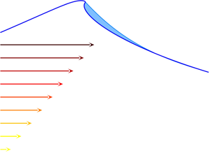
For simplicity, the problem described here is considered to be two-dimensional in the vertical plane. The current field is assumed to be steady, constant in the horizontal  $(x)$ direction, and to vary linearly with depth,
 \begin{equation} U(z)=U_0 + S z. \end{equation}
where  $U_0$ refers to the current velocity at the free surface, and
  $S$ corresponds to its variation with depth. Since 3-D effects are neglected in this study, the vorticity
  $\varOmega$ within the flow is constant, with
  $\varOmega =S$. It is straightforward to show that such a current, associated with the hydrostatic pressure
  $P(z) = p_0 - \rho gz$, is a solution of the Euler equations when considering a problem of constant depth,
  $\rho$ being the density of water, and
  $g$ the acceleration due to gravity. Thus, wavy perturbations can be assumed in the form of a velocity field
  $(u(x,z,t),v(x,z,t))$, associated with the pressure field
  $p(x,z,t)$. The total flow fields are then given by
 \begin{equation} \left. \begin{gathered} \tilde{u}(x,z,t) = u(x,z,t) + U(z), \\ \tilde{v}(x,z,t) = v(x,z,t) \quad \mbox{and} \\ \tilde{p}(x,z,t) = p(x,z,t).\end{gathered}\right\} \end{equation}
Using this decomposition, the Euler equations reduce to
 \begin{gather} u_t + (U+u)u_x + v U_z + v u_z ={-}\frac{p_x}{\rho} \quad \mbox{and} \end{gather}
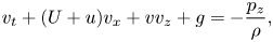 \begin{gather}v_t + (U+u)v_x + v v_z + g ={-}\frac{p_z}{\rho}, \end{gather}
which has to be satisfied together with the continuity equation
 \begin{equation} u_x+v_z=0. \end{equation}
As demonstrated in Simmen (Reference Simmen1984), and more recently in Nwogu (Reference Nwogu2009), the wavy perturbations propagating in such current conditions are irrotational. Indeed, since the second derivative of the background current  $U_{zz}$ is zero, the vorticity conservation equation involves no source term, and the vorticity field does not exchange any vorticity with the wavy perturbations. Yet, it should be emphasized that the presence of constant non-zero vorticity in the background flow might be responsible for substantial changes in the dynamical phenomena, even when considering classical scenario of symmetric travelling water waves. An interesting illustration of such changes is provided by the appearance of the so-called Kelvin cat's eye patterns, which correspond to the occurrence of flow reversal within the orbital velocity field. Discussion of these patterns can be found in Constantin, Strauss & Varvaruca (Reference Constantin, Strauss and Varvaruca2016) and Dyachenko & Hur (Reference Dyachenko and Hur2019). However, provided the absence of exchange of vorticity between the mean flow and the wavy flow, we can introduce a velocity potential
  $\phi (x,z,t)$ from which to derive the perturbation induced velocities (
 $\boldsymbol {\nabla } \phi =(u,v)$). It is emphasized that the continuity equation (2.5) is automatically satisfied if the velocity potential is a solution of Laplace's equation
 \begin{equation} {\rm \Delta} \phi=0.\end{equation}
The kinematic free surface condition can also be expressed, and if  $( X,Z )$ denotes the location of a fluid particle at the free surface, this condition might be expressed
 \begin{equation} \frac{\textrm{d} X}{\textrm{d} t}=u \quad \mbox{and} \quad \frac{\textrm{d} Z}{\textrm{d} t}=v - U(\eta) \frac{\partial \eta}{\partial x}, \end{equation}
where  $\textrm {d}/\textrm {d} t$ refers to the material derivative
  $\textrm {d}/ \textrm {d} t=\partial / \partial t + u \partial /\partial x + v \partial /\partial z$ and
  $Z=\eta (x,t)$.
A streamfunction  $\psi$ can also be introduced, so that
 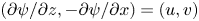 $( \partial \psi /\partial z, - \partial \psi /\partial x) = ( u,v )$. The Euler equations (2.3) and (2.4) can now be integrated in space, giving
 \begin{equation} \frac{\partial \phi}{\partial t} + U(z) \frac{\partial \phi}{\partial x} + \frac{\boldsymbol{\nabla} \phi^2}{2} -S \psi +g z ={-}\frac{p}{\rho}. \end{equation}
When applied to the free surface, where the pressure is constant, this equation provides the classical dynamic boundary condition. Introducing the material derivative used in the kinematic condition, this condition reduces to
 \begin{equation} \frac{\textrm{d} \phi}{\textrm{d} t} + U(\eta) \frac{\partial \phi}{\partial x} - \frac{\boldsymbol{\nabla} \phi^2}{2} - S \psi +g \eta = 0. \end{equation}
At this point, the knowledge of the streamfunction  $\psi$ at the free surface is still needed. We note the relationship
 \begin{equation} \frac{\partial \psi}{\partial \tau}={-} \frac{\partial \phi}{\partial n}, \end{equation}
where  $( \boldsymbol {\tau },\boldsymbol {n} )$ refer respectively to the tangential and normal vectors at the free surface. Thus, the streamfunction
  $\psi$ can be evaluated at the free surface as soon as the normal derivative of the velocity potential is known.
2.2. Numerical solution
The numerical approach used to solve this set of equations is based on a boundary integral element method (BIEM) coupled with a mixed Euler–Lagrange procedure. At each time step, Green's second identity is discretized to solve numerically the Laplace equation (2.6). Thus, the potential and its normal derivative are known numerically, and the streamfunction  $\psi$ can be deduced by integration of (2.10) along the free surface. This numerical integration is performed in the up-wave direction, starting from the down-wave end of the basin and using zero as initial value. Then, the time stepping is performed by numerical integration of (2.7a,b) and (2.9) using a fourth-order Runge–Kutta scheme. Full details of the implementation can be found in Touboul & Kharif (Reference Touboul and Kharif2010). The method has already been implemented and used successfully in the framework of focusing wave groups in the presence of uniform current (Touboul, Pelinovsky & Kharif Reference Touboul, Pelinovsky and Kharif2007; Merkoune et al. Reference Merkoune, Touboul, Abcha, Mouazé and Ezersky2013), or uniform vorticity (Touboul & Kharif Reference Touboul and Kharif2016; Kharif et al. Reference Kharif, Abid and Touboul2017).
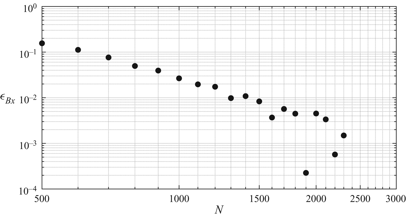
In these previous studies, extensive testing and validation of the methodology were performed. Nonetheless, given the precision required for the present study, a convergence test was conducted, and the results are presented in figure 1. A nearly breaking, recurrent wave packet was propagated in the absence of vorticity. The maximum value of the parameter  $B_x$, as defined by (2.14), was computed. Figure 1 shows the relative error for the results obtained as a function of the number of nodes used to describe the free surface numerically. Given these results, all the simulations conducted within this study involved
  $1500$ nodes, with a numerical time step of
  $dt=10^{-2}$. This corresponds to an average of
  $150$ nodes per wavelength. This choice reduces the relative numerical error to less than
  $1\,\%$ when computing key parameters of the study.

Figure 1. Evolution of the relative error on the maximum value of the breaking parameter  $B_x$ for the maximum recurrent wave as a function of the number of nodes used in the simulation.
For the final stages of the simulations, a partially automated mesh refinement/time- splitting algorithm was used, leading the local value of  ${\textrm {d} x}$ to evolve from
  ${\textrm {d} x}=5.10^{-2}$ to
  ${\textrm {d} x}=5.10^{-4}$, and the time step to reduce to
  $\textrm {d} t=10^{-4}$. Thus, the breaking onset was confirmed for each identified breaking case without any ambiguity. The criterion adopted for confirming breaking onset was the occurrence of a multi-valued surface elevation of the deforming crest, featuring a transient vertical tangent segment.
2.3. Hydrodynamical conditions
The present study considers chirped wave packets, as defined by Song & Banner (Reference Song and Banner2002)
 \begin{align} X_p (t) &={-} 0.25 A_p \left( 1+\tanh \left( \frac{4 \omega_pt}{N {\rm \pi}} \right) \right) \left( 1 - \tanh \left( \frac{4 \left( \omega_p t - 2 N {\rm \pi}\right)}{N{\rm \pi}} \right) \right) \nonumber\\ & \quad \sin \left( \omega_p \left( t - \frac{\omega_p C_{ch} t^2}{2} \right) \right). \end{align}
In the equation above,  $A_p$ refers to the wave packet amplitude,
  $\omega_p$ the average angular frequency of the waves, and
  $N$ is the number of waves present in the packet. Each wave packet is propagated numerically, considering various background flow conditions. Since the purpose of this work is to emphasize the role of vorticity on the marginal breaking criterion, the parameter
  $U_0$ is disregarded, and kept constant at
  $0$. Thus, the current variability in this study relies on a single parameter,
  $S$, providing a depth varying background current distribution according to (2.1). Besides, two values of the normalization length scale,
  $k_p={\rm \pi}$ and
  $k_p={\rm \pi} /2$ are considered in this study. These values provide wave trains propagating, respectively, in deep water conditions and at intermediate water depth. The values of the associated depth parameters are respectively
  $kh=2{\rm \pi}$ and
  $kh={\rm \pi}$. Two carrier wave peak frequencies
  $\omega _p$ are considered, taking the values
  $\omega _p=2{\rm \pi}$ and
  $\omega _p=4{\rm \pi}$ for the sake of normalization. Thus, in both cases, the peak linear carrier wave phase velocity
  $c_0$ is then fixed, with the value
  $c_0=2$.
In this study, the values of  $S$ investigated correspond to moderate values of the vorticity in relation to the wave orbital velocities. For example, the current velocity associated with the background shear current corresponding to
  $S = 1.0$ has a velocity at the maximal crest elevation comparable with the orbital velocity of the steepest non-breaking waves.
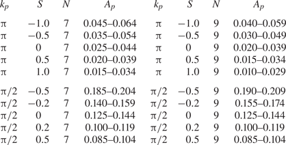
Finally, the parameters used within the study are  $N$, a measure of the bandwidth of the chirped group, and
  $A_p$, its initial amplitude. For a given choice of parameters (
 $S, N$), the wave amplitude
  $A_p$ is varied incrementally in order to capture as accurately as possible the transition between the steepest recurrent wave group and the least steep breaking group. An increment of
  $\delta A_p = 10^{-3}$ was used to quantify the upper and lower transition boundaries separating recurrent and breaking wave packets. A list of the simulations performed is presented in table 1.
Table 1. Hydrodynamical conditions and wave group properties simulated.

2.4. Post-processing of the data
For a given set of parameters  $(S, N, A_p)$, each simulation produces a set of data describing the free surface evolution. These data are post-processed to obtain accurate estimation of the prescribed quantities. Firstly, a wave detection algorithm is introduced, identifying the time evolution of each carrier wave in the packet. The waves, and more specifically their crests, are defined by their corresponding zero up-crossing and the zero down-crossing abscissa,
  $x_{zuc}(t)$ and
  $x_{zdc}(t)$ respectively. Their crest location
  $x_c(t)$ and its time evolution are easily obtained, together with the wave amplitude
  $A_c(t)$.
The instantaneous phase velocity is defined as the time derivative of the crest location,  $c_x=\textrm {d} x_c/ \textrm {d} t$, for each wave crest. This point is crucial, since the parameters used in this study depend strongly on the accuracy used to compute the local phase velocity. For instance, an elegant procedure introduced by Seiffert, Ducrozet & Bonnefoy (Reference Seiffert, Ducrozet and Bonnefoy2017), based on the Hilbert transform of the free surface, provides a local wavenumber, which they link to a local phase velocity by means of the linear dispersion equation. This approach was initially considered for this study, but while computationally efficient, it turned out to be sensitive to the filtering procedure used to estimate the Hilbert transform. Phase velocities computed through this procedure were found to differ by up to
  $40\,\%$ in comparison with the direct computations that we adopted.
For kinematics purposes, we introduce a mean crest location,  $x_{zc}(t)$, defined by the mean location of the two zero crossings,
  $x_{zuc}$ and
  $x_{zdc}$, namely
 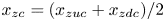 $x_{zc}=( x_{zuc} + x_{zdc} )/ 2$. Its velocity is obtained from
 \begin{equation} c_{zc}=\frac{\textrm{d} x_{zc}}{\textrm{d} t}. \end{equation}
It is also straightforward to define a local crest steepness 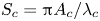 $S_c={\rm \pi} A_c/\lambda _c$, where
  $\lambda _c$ is a characteristic wavelength scale, defined by the distance between the two zero crossings
  $x_{zuc}$ and
  $x_{zdc}$.
Following Barthelemy et al. (Reference Barthelemy, Banner, Peirson, Dias and Allis2016), a leaning parameter  $L$ was also introduced, defined as
 \begin{equation} L=2\frac{x_c-x_{zdc}}{x_{zuc}-x_{zdc}} - 1. \end{equation}
This parameter takes the value  $1$ for a wave presenting a vertical front on its forward face, and the value
  $-1$ for a wave presenting a vertical front on its rear face. Finally, accordingly to the definition introduced by Barthelemy et al. (Reference Barthelemy, Banner, Peirson, Fedele, Allis and Dias2018), we considered the ratio between the local energy flux normalized by the local energy density and the local crest speed. On the wave surface, this quantity simplifies to the ratio of fluid speed
  $u_x$ to crest speed
  $c_x$. Thus, at the surface, it reads
 \begin{equation} B_x=\frac{u_x}{c_x}. \end{equation}
As an aside, we note that in the framework of linear theory, this value further reduces to  $B_x=S_c$.
3. Results and discussion
3.1. Kinematics of marginally recurrent wave groups
Firstly, the influence of vorticity on the kinematic behaviour of these marginally recurrent chirped wave groups is investigated in the neighbourhood of their maximum amplitude location. Results are presented in figure 2. The four panels of this figure describe the time evolution of the kinematic parameters introduced in § 2.4, for an  $N7$ wave packet propagating with or without vorticity. Panel (a) is the local steepness
  $S_c$,(b) is the leaning parameter
  $L$, (c) corresponds to the phase velocity
  $c_{x}$, while (d) depicts the evolution of the velocity of the mean crest location,
  $c_{zc}$, which is defined by (2.12).
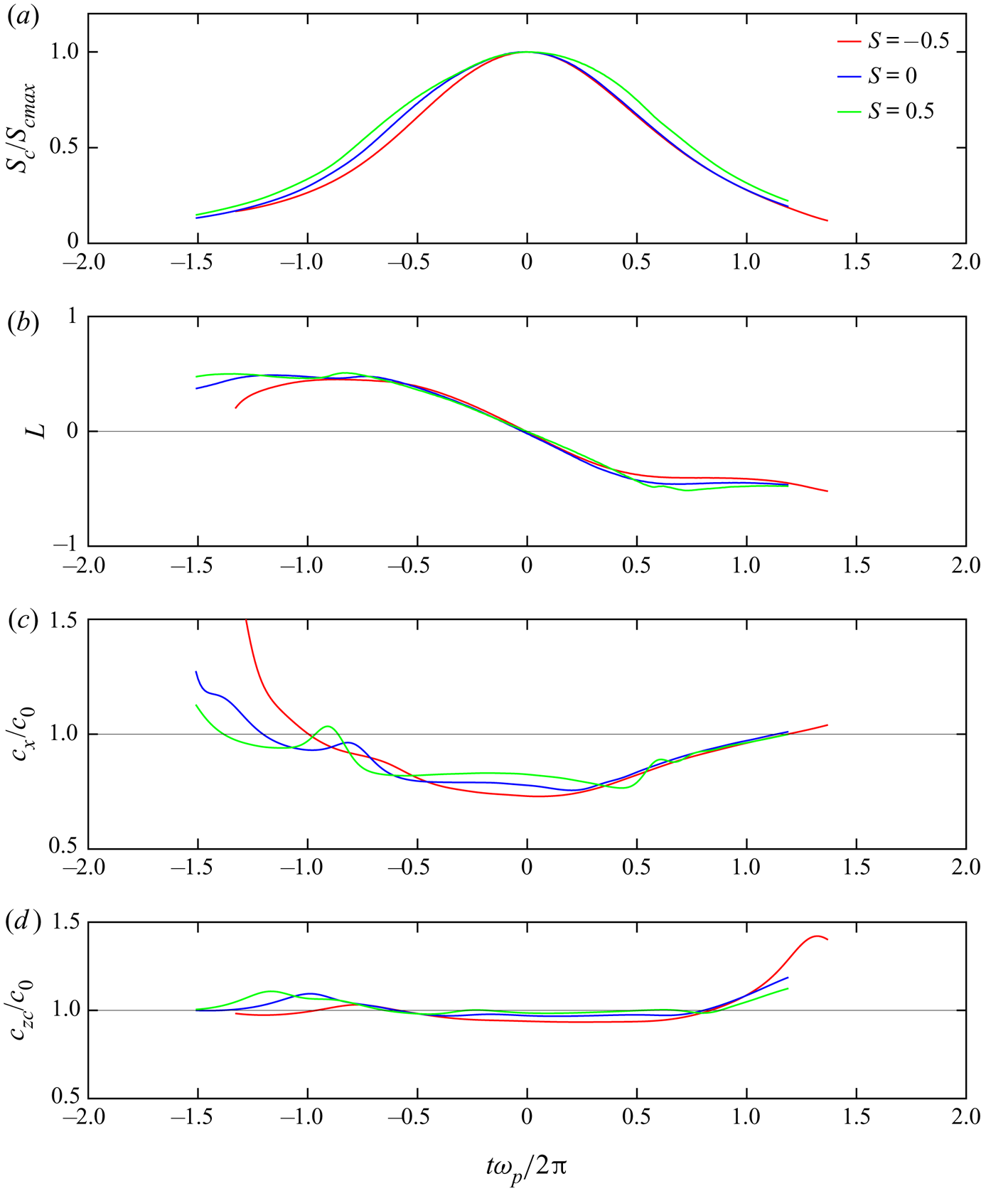
Figure 2. Time evolution of the normalized wave properties, while tracking a marginally recurrent  $N7$ wave packet,
  $k_p={\rm \pi} /2$, propagating with or without initial vorticity. (a) shows the normalized local wave steepness
  $S_c/S_{cmax}$, (b) shows the leaning factor
  $L$, (c) shows the crest velocity
  $c_x/c_0$, while (d) corresponds to the mid-point zero-crossing velocity
  $c_{zc}/c_0$.
The first striking result concerns the significant role played by vorticity on the kinematics of the process. While this influence is seen in the results presented in figure 2, its importance becomes highlighted in the appreciable change that can arise in the limiting wave height at breaking, as is seen in figure 6 below. Indeed, vorticity is known to play a significant role in the focusing time (see e.g. Touboul & Kharif Reference Touboul and Kharif2018). However, the kinematic behaviour observed in previous studies (Fedele Reference Fedele2014; Barthelemy et al. Reference Barthelemy, Banner, Peirson, Dias and Allis2016) is reproduced here when waves propagate in the absence of vorticity. Indeed, when approaching the breaking inception threshold, the steepness of the tallest wave in the group maximizes, after which the steepness begins to decrease. This is accompanied by a generic leaning motion, where the wave crest region, which leans forward  $(L > 0)$ at the early stages of the focusing, maximizes and then decreases, transitioning to leaning backwards
  $(L<0)$ when the wave crest location
  $x_c$ exceeds the mean crest location
  $x_{zc}$. This behaviour corresponds to an initial strong increase of the crest velocity
  $c_x$, followed by a significant, generic slowdown as the crest attains its maximum value. These local changes in the crest velocity can amount to
  $20\,\%$ of the linear theory phase speed
  $c_0$. However, we note that the mean crest velocity,
  $c_{zc}$, which describes an ‘average’ propagation speed of the waveform, shows a behaviour much closer to linear theory, confirming the similar finding in Banner et al. (Reference Banner, Barthelemy, Fedele, Allis, Benetazzo, Dias and Peirson2014).
In the presence of vorticity, the values of these four parameters are modified, but not substantially. The evolution of the crest steepness,  $S_c$, is changed slightly due to asymmetry associated with the sign of the vorticity. In comparison with the zero vorticity evolution, with respect to the maximum steepness location, negative background vorticity delays the initial crest steepening phase and then reduces the rate at which the crest steepness declines after it maximizes. The opposite occurs for positive background vorticity. The minimum leaning value reached by
  $L$ is also affected, the backward-leaning motion being stronger for positive vorticity, and smaller for negative vorticity. Similar observations can be made for both velocities
  $c_x$ and
  $c_{zc}$. Overall, it is interesting to note that the general behaviour described above is not qualitatively affected by the presence of vorticity, with the generic leaning motion of the wave crest little changed.
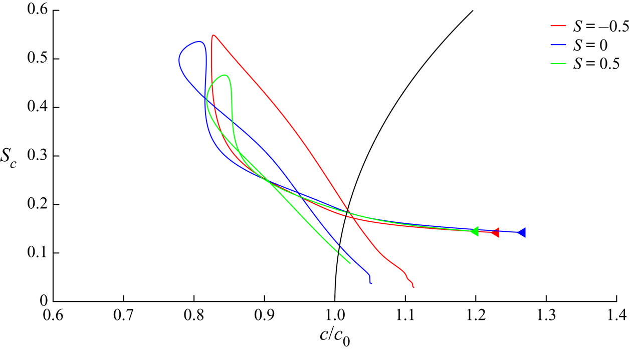
Figure 3 revisits these results in a slightly different manner. Indeed, this figure shows the time evolution of the wave crest in the parameter map provided by  $(S_c,c_x/c_0)$. Each trajectory corresponds to an individual crest lifecycle. The arrow indicates the beginning of the trajectory. For reference, the fifth-order Stokes wave dispersion equation is also plotted in this parameter map. Firstly, it is confirmed that, in such chirped wave groups, the crest velocity does not depend strongly on the local steepness. Remarkably, this result extends to the cases involving vorticity. Secondly, during this marginal recurrent cycle, each crest velocity reduces to a value close to
  $80\,\%$ of the linear phase velocity
  $c_0$, for times which do not necessarily correspond to the maximum steepness reached. In the absence of vorticity, a loop is observed, showing the existence of hysteresis behaviour. In the presence of vorticity, the trajectories might be affected, since the phasing of the slowdown of the crest, with respect to the maximum steepness, is modified. In the presence of positive vorticity, or in the absence of vorticity, the crest slows down, reaches its maximum steepness value and then keeps slowing down, finally reaching its slowest celerity at a steepness lower than the maximum value. It then re-accelerates while the steepness continues to decrease. In the presence of negative vorticity, on the other hand, the minimum crest velocity and maximum steepness are reached at the same instant, and the crest re-accelerates while the steepness starts decreasing. In every case, a hysteresis behaviour is observed, but its phasing is affected by the vorticity.

Figure 3. Time evolution of the local steepness  $S_c$, while tracking a marginally recurrent
  $N7$ wave packet,
  $k_p={\rm \pi} /2$, plotted versus crest celerity, for the maximum recurrent wave obtained with or without vorticity. Black solid line corresponds to the fifth-order Stokes theory.
3.2. Inception of breaking
In figure 4, the time evolution of the breaking parameter  $B_x$, as defined by (2.14), is presented. The figure compares this evolution for marginally recurrent
  $N7$ wave groups, propagated in the presence of positive vorticity
  $S=0.5$, negative vorticity
  $S=-0.5$ and with no vorticity
  $S=0$. Here again, previous results from Barthelemy et al. (Reference Barthelemy, Banner, Peirson, Fedele, Allis and Dias2018) are confirmed in the absence of vorticity, and generalized when vorticity is involved. Indeed, the recurrent wave group evolution generates important fluctuations of the breaking parameter
  $B_x$, also when vorticity is present. If this parameter overshoots the breaking inception threshold value located at
 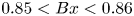 $0.85 < Bx < 0.86$, the wave group will evolve to breaking. Whenever its evolution maintains it beneath the threshold value, the wave group will remain recurrent.
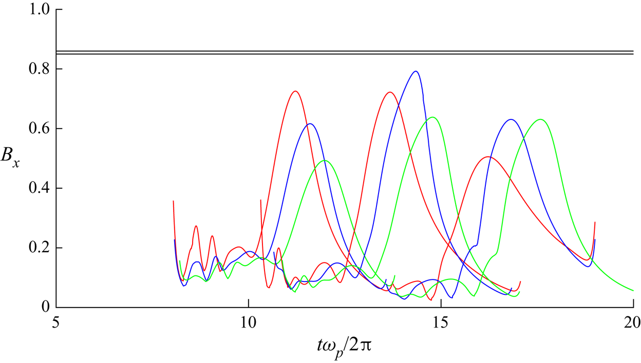
Figure 4. Evolution of the breaking parameter  $B_x$ as a function of time for recurrent wave groups obtained with or without vorticity. The horizontal black lines at
  $0.85 < B_x < 0.86$ are the threshold which segregates breaking from non-breaking cases.
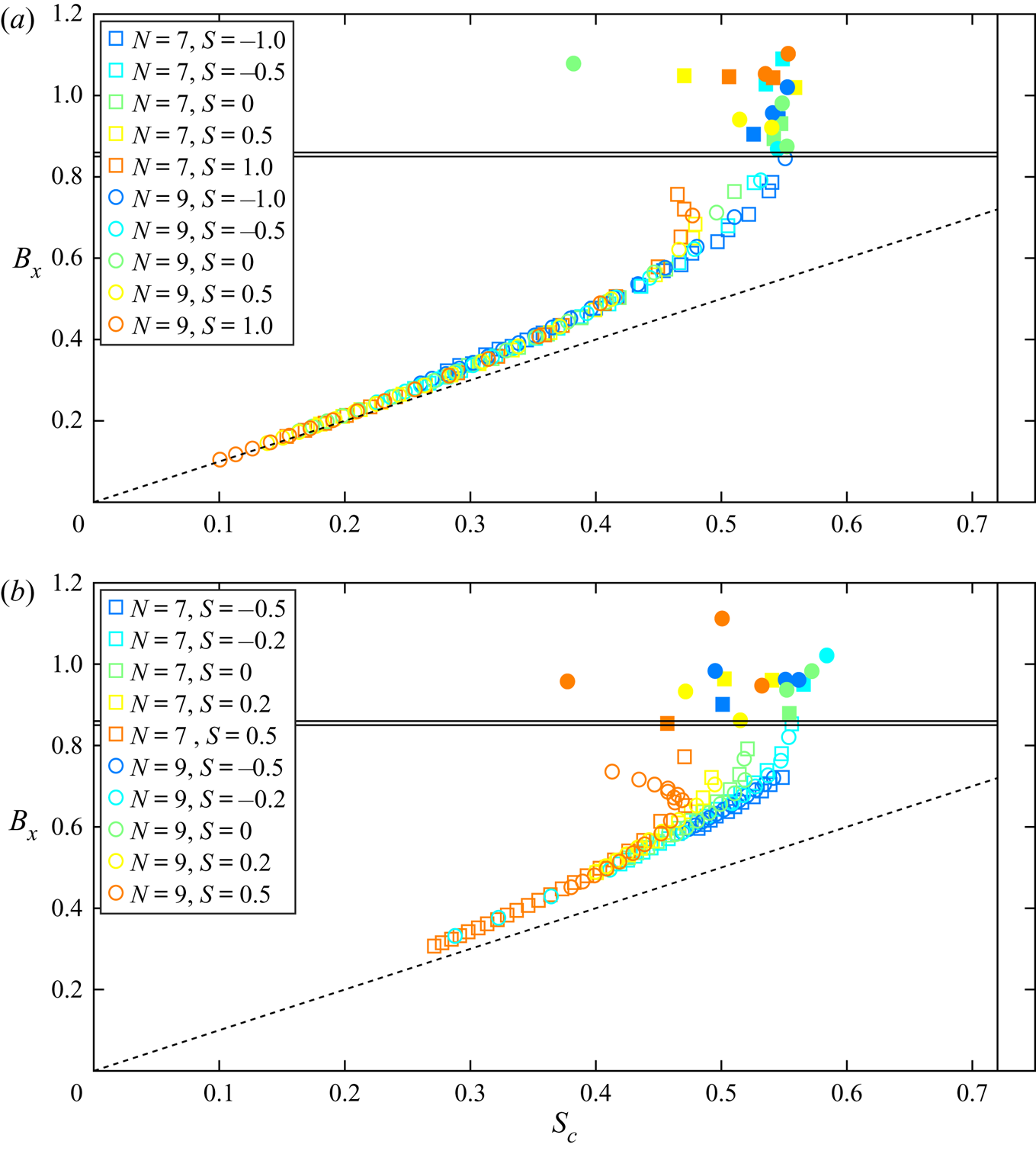
The results summarizing each simulation computed in this study are presented in figure 5. In this figure, each point corresponds to the maximum value of  $B_x$, plotted against the corresponding value of
  $S_c$, for each wave during a modulation cycle. Every simulation run for this work is presented here. When breaking occurred, the symbol is filled, and it is open when the wave packet was recurrent. In addition, the two horizontal black lines, located at
 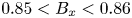 $0.85 < B_x < 0.86$, correspond to the breaking inception threshold identified by Barthelemy et al. (Reference Barthelemy, Banner, Peirson, Fedele, Allis and Dias2018), while the vertical line at
  $S_c=0.72$ is the classical limiting steepness that corresponds to the highest amplitude Stokes wave obtained in deep water. Finally, the black dashed line corresponds to the linear relation
  $B_x=S_c$, which tends to be valid for the smallest waves. From this figure, it is clear that the breaking inception criterion proposed by Barthelemy et al. (Reference Barthelemy, Banner, Peirson, Fedele, Allis and Dias2018) still holds in the presence of vorticity. While vorticity seems to have an impact on the location of waves in this plot, it is clear that this limit still segregates breaking waves from non-breaking ones. This result constitutes the major finding of this study – that the breaking criterion recently proposed by Barthelemy et al. (Reference Barthelemy, Banner, Peirson, Fedele, Allis and Dias2018) is also able to predict wave breaking inception generically for waves propagating in the presence of constant vorticity.

Figure 5. Breaking parameter  $B_x$ plotted against local steepness
  $S_c$. Each point was obtained by tracking the maximum
  $B_x$ for every crest in each wave packet simulated. The horizontal black lines at
  $0.85 < B_x < 0.86$ are the threshold which segregates breaking from non-breaking cases. The vertical line located at
  $S_c>0.72$ corresponds to the classical Stokes corner in deep water conditions. The dashed line is the linearization
  $B_x=S_c$. Top: deep water conditions (
 $k_p={\rm \pi}$), Bottom: intermediate water depth (
 $k_p={\rm \pi} /2$).
3.3. Breaking waves
At first sight, it might be concluded that vorticity does not play a significant role in the dynamics of wave breaking when induced through dispersive focusing. Hence, it is interesting to examine the free surface deformation for a marginally breaking wave group. Figure 6 presents several snapshots of the free surface for two typical cases. Plots in the left column panels are obtained by propagating a  $N9$ wave packet of initial amplitude
  $A_p = 0.046$ with a negative vorticity
  $S=-0.5$. The plots in the central column panels show the evolution of the free surface obtained by propagating a N9 wave packet of initial amplitude
  $A_p = 0.037$ without vorticity
  $S = 0.0$. Finally, the plots in the right column panels correspond to a N9 wave packet of initial amplitude
  $A_p=0.030$ propagated in the presence of positive vorticity
  $S=0.5$. The values of
  $A_p$ were selected to describe the smallest breaking wave packet, for each value of the vorticity. The global trend of
  $A_p$ is thus observed from this analysis. The critical value of
  $A_p$ characterizing the inception of breaking strongly decreases with the increasing value of
  $S$.
$S$.
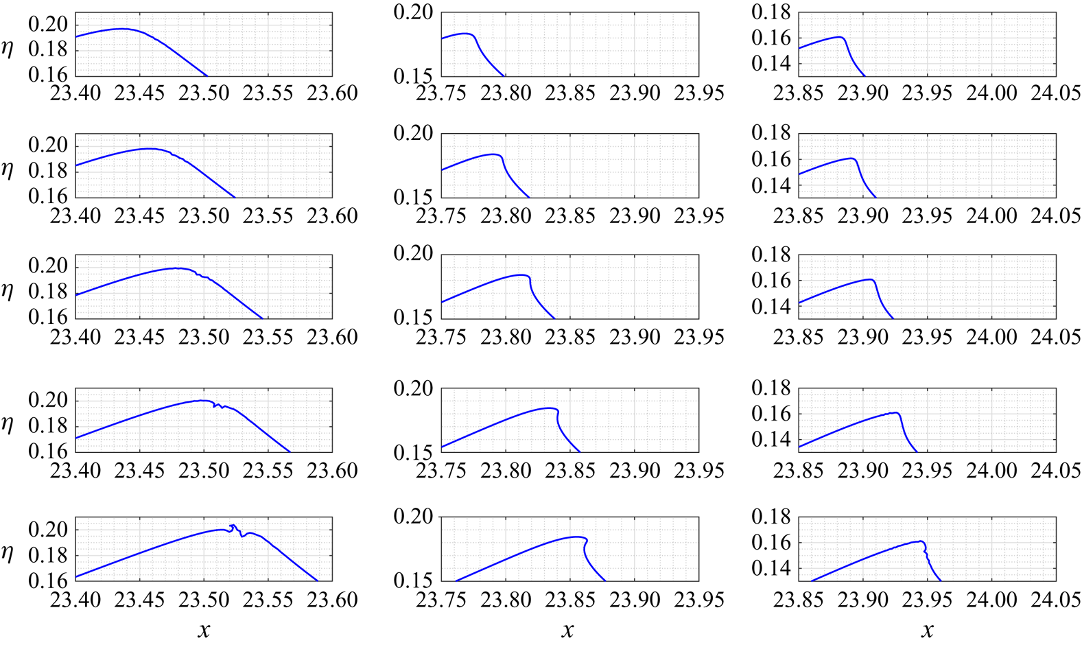
Figure 6. Free surface evolution of a marginal breaking wave obtained by propagating a  $N9$ wave packet. Left-hand panel plots are obtained in the presence of a negative vorticity
  $S=-0.5$, for an initial wave packet of amplitude
  $A_p=0.046$. Centre-panel plots are obtained in the absence of positive vorticity
  $S=0.0$, for an initial wave packet of amplitude
  $A_p=0.037$. Finally, right-side panel plots are obtained in the presence of a positive vorticity
  $S=0.5$, for an initial wave packet of amplitude
  $A_p=0.030$.
When considering the geometry of the breaking wave, it is interesting to note that these three cases exhibit very different behaviours. In the absence of vorticity, or in the presence of positive vorticity, a small jet develops on the front face of the crest, as typically seen in most breaking cases described within the literature. However, the shape of the breaking crest seems to be very different when a negative vorticity is involved. The wave seems to be destabilized initially at the crest, then subsequently on its rear face, where a small jet oriented backwards is developed. This behaviour is very unusual, and, to our knowledge, has not been previously observed. Unfortunately, our BIEM code could not continue to track its further development, and pursuit of this aspect is left to a future study.
4. Conclusions
In this study, chirped deep and intermediate depth water wave packets were produced and propagated numerically by means of a boundary integral element method (BIEM). By varying their initial amplitude, it was possible to investigate the kinematics of the wave crest in the neighbourhood of breaking inception. This study focused on the effect of a uniform vorticity, vertically sheared current on the kinematics and dynamics of water waves approaching breaking inception.
It is found that previous observations describing the crest slowdown and its leaning forward and backward during its amplification cycle, still hold in the presence of vorticity. However, the shape of the breaking crest appears to be significantly affected by the presence of vorticity. For the case of a positively propagating crest within a sufficiently strong negative vorticity field, a small jet appears to form at the rear face of the wave crest, which departs substantially from the familiar forward spilling jet associated with the classical pattern of breaking. Nevertheless, the breaking inception criterion introduced by Barthelemy et al. (Reference Barthelemy, Banner, Peirson, Fedele, Allis and Dias2018) is still found to be valid. Thus this criterion segregates breaking waves from non-breaking waves, even in the presence of a background uniform vorticity field which can significantly distort the wave surface geometry.
Declaration of interest
The authors report no conflict of interest.