2. Formulation

The Boussinesq approach to modelling buoyant flows can be summarised by stating that comparatively minor changes in density are accommodated within the incompressible Navier–Stokes system without changes to fluid properties, such as viscosity and diffusivity. The Boussinesq model is an approximation to the more complete, but computationally expensive, compressible Navier–Stokes system. A standard requirement for good Boussinesq approximations is that the density fluctuations relative to a background density be small, $\rho '/\rho _0\ll 1$ (e.g. see Tritton Reference Tritton1988). With this in mind, the momentum and continuity equations for a Newtonian fluid can be written as

(2.1a,b)\begin{equation} \frac{\rho}{\rho_0}\frac{\mathrm{D}\boldsymbol{u}}{\mathrm{D} t} = \left(1 + \frac{\rho'}{\rho_0}\right)\frac{\mathrm{D}\boldsymbol{u}}{\mathrm{D} t}={-}\frac{1}{\rho_0}\boldsymbol{\nabla}p+\nu\nabla^2\boldsymbol{u}, \quad \boldsymbol{\nabla}\boldsymbol{\cdot} \boldsymbol{u}=0, \end{equation}

where $\mathrm {D}\boldsymbol {u}/\mathrm {D} t$ is the material derivative of velocity, $\rho _0$ is a constant reference density, $\rho '$ is the density fluctuation and $p$ is the pressure. The kinematic viscosity $\nu$ is a constant determined at a temperature corresponding to $\rho _0$. The set (2.1a,b) might be termed the canonical form of the Navier–Stokes–Boussinesq system. A sometimes overlooked fact of Boussinesq-based modelling is that the maximum relative density variation, $\rho '_{max}/\rho _0$, is an independent dimensionless variable and should be sufficiently small for the approximation to be valid.

For general reference frame motion, the material derivative is

(2.2)\begin{equation} \frac{\mathrm{D}\boldsymbol{u}}{\mathrm{D} t} = \frac{\partial\boldsymbol{u}}{\partial t} + \boldsymbol{u}\boldsymbol{\cdot}\boldsymbol{\nabla} \boldsymbol{u} + 2\boldsymbol{\varOmega}\times\boldsymbol{u} + \boldsymbol{\varOmega}\times(\boldsymbol{\varOmega}\times\boldsymbol{r}) + \boldsymbol{\alpha}\times\boldsymbol{r} + \boldsymbol{A}, \end{equation}

where $\partial \boldsymbol {u}/\partial t$ is the local rate of change of velocity, $\boldsymbol {u}\boldsymbol {\cdot }\boldsymbol {\nabla } \boldsymbol {u}$ is its convective rate of change, $\boldsymbol {A}$ is a rectilinear acceleration of the frame origin, $\boldsymbol {\varOmega }$ is frame angular velocity around the origin, $\boldsymbol {\alpha }=\mathrm {d}\boldsymbol {\varOmega }/\mathrm {d} t$ is the angular acceleration of the frame around the origin and $\boldsymbol {r}$ is a position vector relative to the origin. The velocity is measured relative to the frame's origin. The terms $2\boldsymbol {\varOmega }\times \boldsymbol {u}$, $\boldsymbol {\varOmega }\times (\boldsymbol {\varOmega }\times \boldsymbol {r})$ and $\boldsymbol {\alpha }\times \boldsymbol {r}$ are respectively known as Coriolis, centripetal and Euler accelerations. Since acceleration of the origin is a uniform vector field, it can be written as the gradient of a scalar field $\varPhi$ that varies linearly with position, i.e. $\boldsymbol {A}=\boldsymbol {\nabla }(\boldsymbol {A}\boldsymbol {\cdot } \boldsymbol {r})=\boldsymbol {\nabla }\varPhi$. Using standard vector identities, the material derivative may be rewritten as

(2.3)\begin{align} \frac{\mathrm{D}\boldsymbol{u}}{\mathrm{D} t} & = \frac{\partial\boldsymbol{u}}{\partial t} + \boldsymbol{\omega}\times\boldsymbol{u} + \boldsymbol{\nabla} (\tfrac{1}{2}|\boldsymbol{u}|^2 ) + 2\boldsymbol{\varOmega}\times\boldsymbol{u} + \boldsymbol{\nabla} (\tfrac{1}{2}|\boldsymbol{\varOmega}\times\boldsymbol{r}|^2 ) + \boldsymbol{\alpha}\times\boldsymbol{r} + \boldsymbol{\nabla}\varPhi\nonumber\\ & = \frac{\partial\boldsymbol{u}}{\partial t} + \boldsymbol{\omega}\times\boldsymbol{u} + 2\boldsymbol{\varOmega}\times\boldsymbol{u} + \boldsymbol{\alpha}\times\boldsymbol{r} + \boldsymbol{\nabla} (\tfrac{1}{2}|\boldsymbol{u}|^2 + \tfrac{1}{2}|\boldsymbol{\varOmega}\times\boldsymbol{r}|^2+\varPhi ), \end{align}

in which $\boldsymbol {\omega }=\boldsymbol {\nabla }\times \boldsymbol {u}$ is the vorticity. Without loss of generality, a uniform gravitational force per unit mass, $\boldsymbol {g}$, may be replaced by an equivalent frame acceleration $\boldsymbol {A}=-\boldsymbol {g}$, implying also a change in sign of the scalar field $\varPhi$. The gradient term representing centripetal acceleration is often written as $-|\boldsymbol {\varOmega }|^2 \boldsymbol {r}_\perp$, where $\boldsymbol {r}_\perp$ is the radius vector taken perpendicular to the axis of rotation.

A further approximation often applied in concert with that of Boussinesq is to include the effect of density fluctuation only on non-local acceleration terms. This allows density fluctuation effects to be dealt with explicitly in time (as is typically done for the nonlinear terms in uniform-density flows, which is convenient for many time-stepping numerical schemes). Within the context of the canonical Boussinesq approach, this is completely correct for steady flows and approximately so if the local acceleration terms are small compared to the sum of the others. Applying this idea to (2.2), equation (2.3) gives

(2.4)\begin{align} \frac{\rho}{\rho_0}\frac{\mathrm{D}\boldsymbol{u}}{\mathrm{D} t} &\approx \frac{\partial\boldsymbol{u}}{\partial t} + \left(1+\frac{\rho'}{\rho_0}\right)\left[\boldsymbol{u}\boldsymbol{\cdot}\boldsymbol{\nabla}\boldsymbol{u} + 2\boldsymbol{\varOmega}\times\boldsymbol{u} + \boldsymbol{\varOmega}\times(\boldsymbol{\varOmega}\times\boldsymbol{r}) + \boldsymbol{\alpha}\times\boldsymbol{r} + \boldsymbol{A} \right]\nonumber\\ &= \frac{\partial\boldsymbol{u}}{\partial t} + \left(1+\frac{\rho'}{\rho_0}\right) [\boldsymbol{\omega}\times\boldsymbol{u} + 2\boldsymbol{\varOmega}\times\boldsymbol{u} + \boldsymbol{\alpha}\times\boldsymbol{r} + \boldsymbol{\nabla} (\tfrac{1}{2}|\boldsymbol{u}|^2 + \tfrac{1}{2}|\boldsymbol{\varOmega}\times\boldsymbol{r}|^2+\varPhi )]. \end{align}

Since the final group of terms is the gradient of a scalar, (2.4) can be further rearranged in order to remove consideration of hydrostatic-type variations in pressure, to give

(2.5)\begin{equation} \frac{\partial\boldsymbol{u}}{\partial t} + \left(1+\frac{\rho'}{\rho_0}\right) [\boldsymbol{\omega}\times\boldsymbol{u} + 2\boldsymbol{\varOmega}\times\boldsymbol{u} + \boldsymbol{\alpha}\times\boldsymbol{r} ] + \frac{\rho'}{\rho_0} \boldsymbol{\nabla} (\tfrac{1}{2}|\boldsymbol{u}|^2 + \tfrac{1}{2}|\boldsymbol{\varOmega}\times\boldsymbol{r}|^2+\varPhi ). \end{equation}

All forms of (2.4) and (2.5) represent the same rational generalisation of the treatment given by (2.12) of Lopez et al. (Reference Lopez, Marques and Avila2013) in order to deal with arbitrarily accelerating frames of reference. When using this approach in simulations, special treatment or separation of the scalar-gradient-type terms is not required; we have written them as separate terms here partly to aid the exposition below. We point out that Lopez et al. (Reference Lopez, Marques and Avila2013) essentially gave two alternative treatments: one – their (2.4) – for rotating frames of reference with gravity, and the other – their (2.12) – for inertial frames of reference with gravity. The present unified approach can deal with either frame as a special case and it can help explain why using (2.4) and (2.12) of Lopez et al. (Reference Lopez, Marques and Avila2013) will in general give different outcomes if applied to the same flow.

The gradient-type buoyancy-related terms in (2.5) result from: (i) centrifugal buoyancy related to (perhaps localised) swirl with respect to the reference frame, $\boldsymbol {\nabla }(|\boldsymbol {u}|^2/2)$; (ii) centrifugal buoyancy due to uniform frame rotation (sometimes referred to as ‘Coriolis buoyancy’), $\boldsymbol {\nabla }(|\boldsymbol {\varOmega }\times \boldsymbol {r}|^2/2)$; and (iii) buoyancy due to gravity/frame acceleration, $\boldsymbol {\nabla }\varPhi$. The term $\boldsymbol {\nabla }(|\boldsymbol {u}|^2/2)$ is clearly the gradient of kinetic energy per unit mass considered in the frame of reference, and its buoyancy effect does not appear to have an accepted name. However, for flows that are solid-body rotation, considered in an inertial reference frame (such that $\boldsymbol {\varOmega }=0$), it is straightforward to show that it is also associated with centrifugal effects. Note that $\rho '\boldsymbol {\nabla }(|\boldsymbol {u}|^2/2)$ appears as a forcing term in (2.14) of Lopez et al. (Reference Lopez, Marques and Avila2013), who derived it on the basis of an approximation; when considered as an accelerative term rather than a forcing term, it takes the opposite sign to our outcome.

Up to this point we have not discussed how density variations are computed. We use a standard treatment where the relative density variations arise via a constant temperature-dependent volumetric expansion rate $\beta$, such that

(2.6)\begin{equation} \rho'/\rho_0= \beta(T_{ref}-T)=(T_{ref}-T)/T_{ref}, \end{equation}

where $T$ is absolute temperature, $T_{ref}$ is a reference or background value and the latter relation is appropriate to a perfect gas. Very often, $T_{ref}=(T_{hot}+T_{cold})/2$, in which case $\rho '_{max}/\rho _0= (T_{hot}-T_{cold})/(T_{hot}+T_{cold})= \Delta T/(2T_{ref})=\beta \Delta T/2$. To compute transport of temperature, we use an advection–diffusion equation

(2.7)\begin{equation} \frac{\partial T}{\partial t} + \boldsymbol{u}\boldsymbol{\cdot}\boldsymbol{\nabla} T = \kappa\nabla^2 T, \end{equation}

where $\kappa =\nu /{\textit {Pr}}$ is the fluid's thermal diffusivity and $ {\textit {Pr}}$ is the Prandtl number. Equation (2.7) represents the first law of thermodynamics under standard Boussinesq restrictions (see e.g. Tritton Reference Tritton1988). More generally, e.g. for thermohaline buoyancy, more complicated approaches could be used to estimate $\rho '/\rho _0$; provided this remains small, there are no consequences for the key findings of § 3.

In all computations reported in § 3, we have employed a public-domain spectral element code for incompressible flows (Blackburn et al. Reference Blackburn, Lee, Albrecht and Singh2019) and checked that outcomes are effectively resolution-independent. In summary, we solve the (approximate) unsteady incompressible Navier–Stokes–Boussinesq equations

(2.8a,b)\begin{align} &\frac{\partial\boldsymbol{u}}{\partial t} + \left(1+\frac{\rho'}{\rho_0}\right) [\boldsymbol{\omega}\times\boldsymbol{u} + 2\boldsymbol{\varOmega}\times\boldsymbol{u} + \boldsymbol{\alpha}\times\boldsymbol{r} ] + \frac{\rho'}{\rho_0} \boldsymbol{\nabla} (\tfrac{1}{2}|\boldsymbol{u}|^2 + \tfrac{1}{2}|\boldsymbol{\varOmega}\times\boldsymbol{r}|^2+\varPhi )\nonumber\\ &\quad ={-}\boldsymbol{\nabla}\breve{p} + \nu\nabla^2\boldsymbol{u},\quad\boldsymbol{\nabla}\boldsymbol{\cdot}\boldsymbol{u} = 0, \end{align}

where $\breve {p}$ may include hydrostatic variations to the normalised pressure $p/\rho _0$, together with the advection–diffusion equation (2.7), coupled via (2.6). The non-local accelerative terms of (2.8a,b) can be selectively enabled to examine their effects.

In both Marques et al. (Reference Marques, Mercader, Batiste and Lopez2007) and Lopez et al. (Reference Lopez, Marques and Avila2013), it was argued, on the basis that neglected terms should be of second order, that only gradient density-fluctuation effects need be retained in order to obtain first-order-accurate results with Boussinesq-type buoyancy. In what follows we will demonstrate that this may lead to significant error in some cases, even for small density fluctuations. One can choose to include all the buoyancy-related terms in (2.8a,b), or to include only those which factor gradients of a scalar function (effectively, the proposal of Marques et al. (Reference Marques, Mercader, Batiste and Lopez2007), but here generalised to arbitrarily accelerating frames). The difference between these two approaches should only amount to the inclusion or omission of terms in the momentum equations such as

(2.9)\begin{equation} \frac{\rho'}{\rho_0}[ \boldsymbol{\omega}\times\boldsymbol{u}+ 2\boldsymbol{\varOmega}\times\boldsymbol{u} + \boldsymbol{\alpha}\times\boldsymbol{r}] =\frac{\rho'}{\rho_0}[ (\boldsymbol{\omega} +2\boldsymbol{\varOmega})\times\boldsymbol{u} + \boldsymbol{\alpha}\times\boldsymbol{r}], \end{equation}

where $\boldsymbol {\omega }+2\boldsymbol {\varOmega }$ is twice the local fluid rotation rate in the inertial frame. We shall demonstrate that omission of terms (2.9) can have a significant effect on the accuracy of outcomes, though we restrict attention to cases where $\boldsymbol {\alpha }=0$.

3. Numerical results

Our approach is to investigate two simple case studies that possess both rotation and buoyancy, and can be considered in various reference frames, such as in an inertial frame with walls moving relative to the observer, in a rotating frame in which the walls appear fixed, and in an intermediate ‘semi-rotating’ frame. For both case studies, no flow other than solid-body rotation would arise in the absence of centrifugal buoyancy effects. The first test case is an axisymmetric restriction of the flow considered by Marques et al. (Reference Marques, Mercader, Batiste and Lopez2007), while the second is an axially invariant version of the flow configuration considered by Pitz, Marxen & Chew (Reference Pitz, Marxen and Chew2017). Both cases have non-slip walls, so that far-field boundary conditions (and how these might need to account for hydrostatic pressure gradients) do not require detailed examination, and both have $\boldsymbol {\alpha }=0$.

3.1. Axisymmetric steady flow

The first case is the same as that examined in § 3.1 of Marques et al. (Reference Marques, Mercader, Batiste and Lopez2007); axisymmetric flow in a rotating cylindrical container of radius-to-length aspect ratio $R/L=1$, heated on one endwall and cooled on the other, with an adiabatic outer wall. In their treatment, gravitational acceleration acts in the direction pointing from the cool wall to the hot wall, and the Prandtl number ${\textit {Pr}}=7$, i.e. the modelled flow is that of water in a rotating cylinder heated from below. They used $(\rho '/\rho _0)\boldsymbol {\nabla }(|\boldsymbol {\varOmega }\times \boldsymbol {r}|^2/2+\varPhi )$ for the buoyancy terms, $\rho '_{max}/\rho _0=0.031429$, and omitted the gradient of kinetic energy as well as the terms in (2.9). In the absence of centrifugal buoyancy, the basic state consists of uniform conduction and solid-body rotation. For non-zero Froude number, ${\textit {Fr}}=|\boldsymbol {\varOmega }|^2R/|\boldsymbol {g}|$, the saturated states (prior to onset of any instability) are steady toroidal overturning motion with upwelling of warm fluid along the axis and a return flow of cooled fluid near the outer wall. The remaining dimensionless groups (of total six) are: maximum relative density variation $\rho '_{max}/\rho _0$; Rayleigh number ${\textit {Ra}}=\beta |\boldsymbol {g}|L^3(T_{hot}-T_{cold})/\kappa \nu$; and Coriolis number ${\textit {Co}}=|\boldsymbol {\varOmega }|L^2/\nu$.

Figure 1 presents results from our axisymmetric simulation at ${\textit {Fr}}=0.4$, ${\textit {Co}}=100$ and ${\textit {Ra}}=1.1\times 10^{-4}$; the same parameter values as used for the simulation in figure 1 of Marques et al. (Reference Marques, Mercader, Batiste and Lopez2007). The resulting flows are steady, $\partial \boldsymbol {u}/\partial t=0$, in all frames of reference. We take $T_{hot}-T_{cold}=1$, and so in (2.6) $T_{ref}\equiv 15.909$. The flow visualisations shown in figure 1(a–d) are presented in the meridional $(x,r)$ semiplane and rotation is around the $x$ axis; lengths are normalised by the cylinder radius $R$.

Figure 1. Simulation results for the axisymmetric test case of § 3.1 of Marques et al. (Reference Marques, Mercader, Batiste and Lopez2007). Panels (a–d) illustrate flows in the meridional $(x,r)$ semiplane; the cylinder rotates around the $x$ axis. The gravity vector is aligned with the $+x$ axis, or, equivalently, frame acceleration is aligned with $-x$. Colour contours are of $T-T_{ref}$ drawn at levels $-0.5$ to $+0.5$ in steps of 0.1, and dashed lines represent negative values. Sectional streamlines illustrate meridional flows. (a–c) Flows computed using gradient-type buoyancy, respectively in inertial, semi-rotating and fully rotating frames of reference. (d) The same quantities computed using the more complete approach of (2.8a,b) – the same in all frames of reference. (e) Temperature profiles extracted along the axis (inset shows detail around the zero crossings). The solid line shows data from the results of (d); the dotted, chained and dashed lines show data from (a), (b) and (c), respectively; the semi-rotating case (b) differs significantly from the others.

Figure 1(a–c) represent computations made using the gradient-based buoyancy approach, i.e. where the terms of (2.9) are omitted, respectively for the inertial frame of reference (where walls rotate at the vessel rotation rate $|\boldsymbol {\varOmega }|$), the semi-rotating frame (walls rotate at rate $|\boldsymbol {\varOmega }|/2$) and the fully rotating frame of reference (in which the walls appear fixed). One may observe that the results in panels (a) and (c) are much alike, and very similar to those in figure 1 of Marques et al. (Reference Marques, Mercader, Batiste and Lopez2007), while those in panel (b), while superficially similar, differ significantly in detail from panels (a) and (c); note, for example, the locations of the $T=0$ contours (the first solid lines) along the rotation axis, $x$.

Figure 1(d) shows results using the more complete approach where the terms of (2.9) are retained in (2.8a,b). In this case, meridional flows and temperature contours for all three frames of reference are identical to within numerical error (here, at relative levels approximately nine orders of magnitude or more below the outcomes presented). This agreement demonstrates the completeness of the approach advocated in (2.8a,b) for steady flows.

Figure 1(e) shows profiles of temperature extracted along the rotation axis for the various approaches of figure 1(a–d). From these, the locations for $T=0$ on the $x$ axis can be read more precisely. Again, we note the relatively good agreement of panels (a) and (c), and that these agree well with those of panel (d), while results obtained with the gradient-only buoyancy approach in the semi-rotating frame, panel (b), are significantly in error.

3.2. Non-axisymmetric flow

Our second case study is a simple adaptation of the rotating annular cavity flow considered by Pitz et al. (Reference Pitz, Marxen and Chew2017), with a hot outer wall and cold inner wall. This case considers a zero-gravity environment, and so centrifugal buoyancy is wholly responsible for driving azimuthal flow variations. We focus on the geometry with inner-to-outer radius ratio $\eta =a/b=0.52$, as was the case in most of their work. To simplify matters, we compute two-dimensional flows that are axially invariant, while most of their results were for a fully enclosed cavity with adiabatic endwalls. In the absence of gravity and endwalls, the five independent dimensionless groups may be represented as $\eta$, ${\textit {Pr}}$, $\rho '_{max}/\rho _0$, $Re=|\boldsymbol {\varOmega }|(b+a)(b-a)/2\nu$ and ${\textit {Ra}}= \beta (T_{hot}-T_{cold})|\boldsymbol {\varOmega }|^2(b+a)(b-a)^3/2\kappa \nu$. As in Pitz et al. (Reference Pitz, Marxen and Chew2017), we use ${\textit {Pr}}=0.7$ (air) and $\rho '_{max}/\rho _0=0.05$. Pitz et al. (Reference Pitz, Marxen and Chew2017) carried out computations in a rotating frame of reference, included only the gradient-based centripetal acceleration term $(\rho '/\rho _0)\boldsymbol {\nabla }(|\boldsymbol {\varOmega }\times \boldsymbol {r}|^2/2)$ in their approximation to (2.8a,b), and, like Marques et al. (Reference Marques, Mercader, Batiste and Lopez2007), omitted the terms of (2.9). Pitz et al. found that the fully enclosed flow bifurcated to a (standing) wave, steady in the rotating frame, with azimuthal wavenumber $k=5$ at ${\textit {Ra}}=3040$ (see their table 1).

This case is somewhat more complicated than the one considered in § 3.1, largely because of the possibility of unsteady flow at the onset of instability. This enables us to additionally examine the consequences of committing the (standard) modelling approximation error of omitting term $(\rho '/\rho _0)\partial \boldsymbol {u}/\partial t$ from (2.1a,b). We mainly focus on the critical Rayleigh numbers, which are typically substantially smaller than those of Pitz et al. (Reference Pitz, Marxen and Chew2017). This difference is due to the effects of endwalls, which were present for their study, but are absent in ours. We first compute the stable one-dimensional rotating basic state at ${\textit {Ra}}=1500$, add a small white-noise perturbation everywhere in the domain at higher Rayleigh numbers, wait for saturated two-dimensional states to evolve, then reduce the Rayleigh number and repeat until the bifurcation is suitably bracketed. This is detected by subtracting the stable basic state and computing the domain integral of kinetic energy in the difference flow; since the bifurcation is of supercritical Hopf type, this energy integral initially varies linearly with the control parameter, Rayleigh number, at onset (Guckenheimer & Holmes Reference Guckenheimer and Holmes1986). As in the case study of § 3.1, we have carried out simulations in inertial, rotating and semi-rotating frames of reference using both the near-complete approach of (2.8a,b), and the gradient-only approach in which the terms (2.9) are omitted. 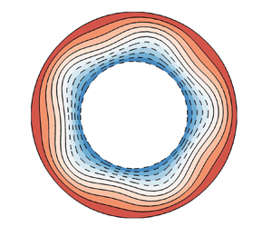In all cases, instability is a supercritical Hopf bifurcation to azimuthal waves with $k=5$. Figure 2 shows a snapshot of temperature contours obtained using the computational technique represented by (2.8a,b), obtained in the fully rotating frame at ${\textit {Ra}}=1850$, illustrating the $k=5$ wave.

Figure 2. Simulation results for a two-dimensional flow in a rotating annulus at ${\textit {Ra}}=1850$, with centrifugal buoyancy. This is an axially invariant equivalent of the annulus of radius ratio $\eta =0.52$ considered by Pitz et al. (Reference Pitz, Marxen and Chew2017). Colour contours of $T-T_{ref}$ range from $-1$ at the inner radius (blue) to $+1$ at the outer radius (red), in steps of 0.2; dashed lines represent negative values.

In table 1, critical Rayleigh numbers ${\textit {Ra}}_c$ for our two-dimensional simulations are presented, along with their percentage variations from the ‘true’ value obtained using the approach of (2.8a,b). (We have refined spatial meshes and time step sizes to the point that relative numerical errors of the values presented are well below the accuracy suggested by the number of significant figures provided.) The solution obtained in the fully rotating frame for the ‘non-gradient’ equation set (2.8a,b) is a slow retrograde rotating wave; its rotation speed relative to the reference frame is $-2.515\times10^{-3}$. We have also carried out a bifurcation study for a frame in which this wave appears fixed, thus making the local accelerations $\partial \boldsymbol {u}/\partial t=0$. This is the ‘true’ reference case from which the errors in ${\textit {Ra}}_c$ shown in table 1 were calculated. To approximately five significant figures, ${\textit {Ra}}_c=1759$ for this case agrees with that obtained for the fully rotating frame of reference when the ‘complete’ approach of (2.8a,b) is employed. In this two-dimensional restriction, ${\textit {Ra}}_c$ is well below that in the full three-dimensional study of Pitz et al. (Reference Pitz, Marxen and Chew2017), and somewhat above the value for Rayleigh–Bénard convection rolls between two parallel planes, ${\textit {Ra}}=1708$ (Chandrasekhar Reference Chandrasekhar1961).

Table 1. Critical Rayleigh numbers, ${\textit {Ra}}_c$, with relative errors, for the non-axisymmetric case study shown in figure 2. $\varOmega$ is the dimensionless rotation rate of the frame of reference used, varying between zero (inertial) and unity (fully rotating). A reference case, with $\varOmega =0.997485$ was used to compute the error values listed (see text).

Considering the differences in estimates of ${\textit {Ra}}_c$ in table 1, we first note that for the inertial and semi-rotating frames, all solutions are rotating waves, and in the inertial frame ($\varOmega =0$), the waves rotate at very close to the rotation rate of the annulus. In the fully rotating frame ($\varOmega =1$) and for the non-gradient approach, the solution is a very slow rotating wave. We have already seen that for the steady flows, as considered in § 3.1, the non-gradient and the more complete Boussinesq approximations produce identical results (modulo solid-body rotation) in all frames. Thus we can attribute the increasing error in ${\textit {Ra}}_c$ as $\varOmega$ decreases for the non-gradient results listed in table 1 to the fact that $(\rho '/\rho _0)\partial \boldsymbol {u}/\partial t$, a term neglected in all our and, as far as we are aware, all extant Boussinesq approximations, becomes more important when the flow becomes increasingly unsteady as $\varOmega$ decreases below 0.997485 towards zero. Provided $\rho '/\rho _0\ll 1$, such errors should always be relatively small. For the present calculations, the maximum error in ${\textit {Ra}}_c$ for the non-gradient approach, 3.7 %, is of the same order as $\rho '_{max}/\rho _0$, 5 %.

Table 1 also shows that, for the gradient-based Boussinesq approximation, errors in ${\textit {Ra}}_c$ are relatively small when $\varOmega =0$ and 1, but very large for the semi-rotating case with $\varOmega =0.5$. This is mainly attributable to omitting the terms represented in (2.9), which are apparently significant for the semi-rotating case. Recall that for the steady flow of § 3.1, the error for the gradient-based approach was also largest in the semi-rotating case. Finally, for $\varOmega =1$ there is a distinction in bifurcation behaviour between the two Boussinesq approaches. While for the non-gradient approach, the bifurcation is to a rotating wave, for the gradient approach, a standing wave bifurcates. Theoretically, if the modelled physics were equivalent, these two wave types would bifurcate linearly at the same value of ${\textit {Ra}}_c$, and (weakly) nonlinear effects would select one of these two outcomes as the stable case, observable using nonlinear simulations. Therefore, changing the modelled physics (from non-gradient- to gradient-based buoyancy) here also changes the nature of the bifurcation.