


1. Introduction
The study of spray atomization has numerous applications including combustion, surface coating, pharmaceutical manufacturing and disease transmission modelling. Atomization is conventionally subdivided into two stages: primary atomization, which describes the breakup of the bulk liquid into smaller droplets, and secondary atomization, which describes the further breakup of these droplets. While the study of single-droplet breakup is directly the study of secondary atomization, it can also be applied in models for primary atomization (O'Rourke & Amsden Reference O'Rourke and Amsden1987; Varga, Lasheras & Hopfinger Reference Varga, Lasheras and Hopfinger2003; Aliseda et al. Reference Aliseda, Hopfinger, Lasheras, Kremer, Berchielli and Connolly2008). A detailed understanding and accurate modelling of droplet breakup is therefore crucial in the development of spray atomization applications. However, despite extensive experimental and theoretical study, there remains disagreement in the literature as to the underlying physical mechanisms of droplet breakup.
Droplet breakup has been historically categorized into five breakup morphologies, each of which occur at increasing relative air velocity: Bag, bag and stamen (BS), multibag (MB), sheet thinning (ST) and catastrophic (Pilch & Erdman Reference Pilch and Erdman1987; Guildenbecher, López-Rivera & Sojka Reference Guildenbecher, López-Rivera and Sojka2009). In bag breakup, a single bag forms on the leeward side of the droplet, surrounded by a thick liquid rim. Upon breakup, the bag forms very small droplets while the rim breaks into larger ones. The BS morphology is similar to Bag, however, a stamen forms at the centre of the drop, creating a large additional drop during breakup. MB breakup is characterized by the formation of multiple bags across the drop. In ST breakup, the periphery of the drop is deflected downstream and forms a sheet, which breaks into small drops. Images of the characteristic breakup shapes are shown in figure 1. Catastrophic breakup is when the droplet appears to explode into a multitude of fragments and occurs at very high relative velocities.

Figure 1. Images of (a) Bag, (b) BS, (c) MB and (d) ST breakup modes.
It has been previously shown that the breakup morphologies can be classified by the Weber number and the Ohnesorge number (Pilch & Erdman Reference Pilch and Erdman1987) given by (1.1) and (1.2), respectively,
 \begin{gather} We = \frac{\rho_g U^2 d_0}{\sigma} \end{gather}
 \begin{gather}Oh = \frac{\mu_l}{\sqrt{\rho_l \sigma d_0}}, \end{gather}
where  $\rho _g$ and
  $\rho _l$ are the gas and liquid phase densities in kg m
 $^{-3}$,
  $\mu$ is the liquid viscosity in Pa s,
  $\sigma$ is the interfacial surface tension in N m
 $^{-1}$,
  $d_0$ is the initial diameter of the droplet in m and
  $U$ is the relative velocity between the gas and the droplet in m s
 $^{-1}$. A critical Weber number,
  $We_c$, is established for the transition to each morphology. Guildenbecher et al. (Reference Guildenbecher, López-Rivera and Sojka2009) summarize the morphology transitions as
  $We_{c, Bag} \approx 11$,
  $We_{c, BS} \approx 18$,
  $We_{c, MB} \approx 35$ and
  $We_{c, ST} \approx 80$. Comparatively, Zhao et al. (Reference Zhao, Liu, Li and Xu2010) give values of
  $We_{c, Bag} \approx 12$,
  $We_{c, BS} \approx 16$,
  $We_{c, MB} \approx 28$, and
  $We_{c, ST} \approx 80$. This highlights that the morphology transitions are not necessarily discrete and may exist over a small range of
  $We$. Below the limit of
  $We_{c, Bag}$, no breakup (NB) occurs. For
  $Oh<0.01$, the values of
  $We_c$ are unaffected by the liquid viscosity (Hsiang & Faeth Reference Hsiang and Faeth1992).
The overall breakup process of droplets can be subdivided into two basic phases: the initiation phase (sometimes referred to as the deformation phase), and the breakup phase which consists of the growth and breakup of the bags and rims (Pilch & Erdman Reference Pilch and Erdman1987). During the initiation phase, the droplet expands radially and flattens until it forms a disk. At some point, the disk becomes thin enough to be blown into one or more bags surrounded by thick rims. The instant that the bags first form is termed the ‘initiation time’. After the initiation time, the bags grow until they break, causing the rims to break with them into the child droplets. The dimensionless time,  $T$ (1.3), which is non-dimensionalized by the characteristic deformation time,
  $\tau$ (1.4), is conventionally used for scalable analysis of transient droplet breakup
 \begin{gather} T = \frac{t}{\tau} \end{gather}
 \begin{gather}\tau = \frac{d_0}{U} \sqrt{\frac{\rho_l}{\rho_g}} . \end{gather}
Conveniently, the characteristic deformation time defined by Rimbert et al. (Reference Rimbert, Castrillon Escobar, Meignen, Hadj-Achour and Gradeck2020) is identical to the characteristic breakup time due to interfacial instabilities which are commonly related to liquid breakup (Pilch & Erdman Reference Pilch and Erdman1987) and thus can be used to non-dimensionalize many droplet breakup analyses.
Numerical simulations of droplet breakup have been able to provide reasonable qualitative agreement with experiments, mainly with respect to breakup morphologies; however, quantitative agreement in the breakup phase is still lacking. One of the key limitations of these numerical simulations is mesh-induced breakup, which occurs when the mesh size is not fine enough to resolve micro-scale phenomenon. A finer grid is often not feasible due to the computational cost. This causes the simulations to predict a premature breakup of thin fluid structures such as bags, limiting even qualitative agreement near the breakup point (Strotos et al. Reference Strotos, Malgarinos, Nikolopoulos and Gavaises2016). Consequently, there is still a strong focus on improving the methods to achieve better quantitative agreement (Strotos et al. Reference Strotos, Malgarinos, Nikolopoulos and Gavaises2016; Xiao, Dianat & McGuirk Reference Xiao, Dianat and McGuirk2016). Nevertheless, many works seek to use numerical simulations to learn more about the breakup process, particularly at high  $We$ near the transition of ST to catastrophic breakup where the underlying physical mechanisms are largely disputed (Jalaal & Mehravaran Reference Jalaal and Mehravaran2014; Meng & Colonius Reference Meng and Colonius2018; Dorschner et al. Reference Dorschner, Biasiori-Poulanges, Schmidmayer, El-Rabii and Colonius2020).
While numerical simulation is a useful tool with increasing capability for studying droplet breakup, analytical models are more desirable as they provide a clearer insight into the important physical phenomena. Additionally, analytical models are better suited for use in spray modelling where many thousands of droplets must be analysed. The chief goal of these models is to predict the child droplet sizes resulting from the breakup, however, there is also interest in modelling the transitions between the breakup morphologies. Previous analytical modelling attempts can be divided into three main categories: mass–spring–damper analogy models, instability models and internal flow models.
Mass–spring–damper analogy models assume that the droplet acts as a mass–spring– damper system, simplifying the problem to a one-dimensional (1-D) equation that is solved analytically. The most well known of these models is the Taylor analogy breakup (TAB) model (O'Rourke & Amsden Reference O'Rourke and Amsden1987). In these analyses, the restoring force of surface tension acts as the spring and viscosity as the damper to the aerodynamic forces of the gas flow. The breakup of the droplet is predicted to occur when a critical deformation is attained ( $d/d_0 = 1.5$ for TAB), where the drop then fragments such that the deformation energy is transformed to the surface energy of the child droplets. In modelling the breakup in this way, the approach neglects the complex physics of the breakup phase. A significant limitation of the TAB model is that several empirical constants are required to give a complete prediction of the deformation and breakup sizes. Several improvements on the TAB model have been presented in the literature. The ‘enhanced TAB model’ (Tanner Reference Tanner1997) modifies the breakup mechanism to relate the child droplet size to the breakup time. Park, Yoon & Hwang (Reference Park, Yoon and Hwang2002) proposed an ‘improved TAB model’ where the effect of drag on the deformation was considered and the breakup criterion was changed to be based on the pressure distribution across the drop. A notable variant of the mass–spring–damper model is the dynamic droplet breakup model (Ibrahim, Yang & Przekwas Reference Ibrahim, Yang and Przekwas1993) which models the deformation based on an energy approach, however, Lee et al. (Reference Lee, Park, Farid and Yoon2012) find that the model's prediction is inaccurate. Although these models are commonly implemented in industrial fluid dynamics software for low
  $We$ breakup (ANSYS Inc. 2011), the original works are mostly compared against a very small data set from Krzeczkowski (Reference Krzeczkowski1980), which has poor temporal and spatial resolution compared to what is possible with current flow visualization technologies. Furthermore, these models have poor prediction near
  $We_{c, Bag}$ and neglect the various breakup morphologies and the presence of rim and bag geometries in the breakup.
Instability models apply surface instability theories, mainly the Rayleigh–Taylor inertial instability, to the face of a flattened droplet. Notable examples of these works include Harper, Grube & Chang (Reference Harper, Grube and Chang1972), Liu, Mather & Reitz (Reference Liu, Mather and Reitz1993), Joseph, Beavers & Funada (Reference Joseph, Beavers and Funada2002), Theofanous, Li & Dinh (Reference Theofanous, Li and Dinh2004) and Zhao et al. (Reference Zhao, Liu, Li and Xu2010). In these analyses, the instability is related to the breakup mechanism by the number of wavelengths,  $\lambda$, of the most unstable surface wave that fit on the face of the flattened drop of diameter
  $d$. NB, Bag, BS and MB breakup are supposed to occur at
  $\lambda /d < 1$,
  $1 < \lambda /d < 2$,
  $2 < \lambda /d < 3$ and
  $\lambda /d > 3$, respectively (Zhao et al. Reference Zhao, Liu, Li and Xu2010). For these analyses, it is necessary to determine
  $d$, which is most often taken from empirical correlations such as Hsiang & Faeth (Reference Hsiang and Faeth1992), although the mass–spring–damper deformation models described above have also been used as in Liu et al. (Reference Liu, Mather and Reitz1993). Even in the cases where the deformation models are used in the prediction, the instability theories largely disregard the importance of the flow dynamics prior to the formation of the flattened disk as they are only concerned with determining its critical size. Additionally, in order to determine
  $\lambda$, the acceleration of the droplet must be found based on the drag coefficient of the droplet,
  $C_d$, which changes throughout the deformation. As a result, an additional assumption must be made about
  $C_d$, which is taken either from empirical correlations, the limiting disk geometry (Zhao et al. Reference Zhao, Liu, Cao, Li and Xu2011a), or by linear interpolation between a sphere and disk (Liu et al. Reference Liu, Mather and Reitz1993), which cyclically depends on the deformation. In the majority of these analyses, the instability theories were developed for infinite planes of semi-infinite thickness while the droplets themselves are finite planes of finite thickness, bringing into question the validity of their use. While the finite-thickness problem has been studied by Keller & Kolodner (Reference Keller and Kolodner1954) and implemented by Jain et al. (Reference Jain, Prakash, Tomar and Ravikrishna2015), the effect of the finite boundary of the droplet periphery on the instability has not been considered. Since the droplet periphery is of the same order of magnitude as the instability wavelength, it is plausible that the droplet periphery has a significant effect on the nature of the instability. Although this method has been found to provide reasonable prediction of
  $We_c$ for the Bag, BS and MB morphologies, the omittance of these properties brings into question its applicability to the problem as noted by Jain et al. (Reference Jain, Prakash, Tomar and Ravikrishna2015). Additionally, the instability theory has not been shown to be able to predict the relevant geometries of low
  $We$ breakup such as the rims, or the child droplet sizes that result from their breakup. Despite these shortcomings, surface instabilities are currently the prevailing theory in the literature for the dynamics of low
  $We$ droplet breakup.
The internal flow mechanism suggests that the drop deformation results from the flow of liquid from the poles of the drop to its equator. The resistance due to surface tension at the equator then causes the formation of the rim. When the liquid flow becomes strong enough to resist the surface tension, the equator will thin indefinitely and be susceptible to being drawn downstream, leading to the ST morphology. Although this mechanism was first qualitatively described by Guildenbecher et al. (Reference Guildenbecher, López-Rivera and Sojka2009) in an effort to provide a physical explanation of the transition to ST, no quantitative analysis was given. Villermaux & Bossa (Reference Villermaux and Bossa2009) modelled the internal flow of a drop in the bag breakup regime by solving the axisymmetric Euler equation for the 1-D radial flow in the drop due to a stagnation-point flow on its windward face. This internal flow gave the initial deformation of the drop's equator, which was linked to the thinning of the droplet and thus to the growth of the bag by a force balance. The result is a 1-D equation that can be solved numerically to predict the deformation of the droplet and the growth of the bag. Although good agreement is shown for the bag growth model to the small data set presented in Villermaux & Bossa (Reference Villermaux and Bossa2009), the model is limited in that it does not directly relate the droplet deformation and bag growth phases to the droplet breakup and is applicable only for the Bag morphology. Although Villermaux & Bossa (Reference Villermaux and Bossa2009) provide a child droplet size prediction, it is essentially a fit of a gamma distribution to breakup size data and neglects the deformation component of the model. Kulkarni & Sojka (Reference Kulkarni and Sojka2014) carried out the same analysis including viscous effects in the deformation and surface tension effects in the bag growth portions of the model, however, these effects were negligible for their experimental range (note that an error in this model was corrected by Stefanitsis et al. Reference Stefanitsis, Strotos, Nikolopoulos, Kakaras and Gavaises2019). The model of Kulkarni & Sojka (Reference Kulkarni and Sojka2014) provides poor prediction near  $We_{c,Bag}=12$, where their model transitions from an oscillatory solution to one of infinite growth. Mashayek & Ashgriz (Reference Mashayek and Ashgriz2009) modelled the deformation of the droplet surface using the 2-D axisymmetric Navier–Stokes equations. The pressure distribution on the drop surface was provided using a perturbation analysis about a trivial zeroth-order solution based on the drag coefficient of a sphere. This method gives a prediction of the 2-D drop topology which better represents the actual droplet shape throughout the deformation. Although these models used the internal flow theory to describe the dynamics of droplet deformation, none were able to link this phase to the breakup sizes or morphology. Furthermore, the models were only compared against a very limited dataset within a narrow range of
  $We$. Consequently, the internal flow mechanism has not yet been widely adopted.
Although there have been many attempts to model the breakup of droplets, no analytical model has been developed that describes and predicts both the breakup morphology and the child droplet sizes for a wide range of conditions. Models which are capable of predicting the droplet breakup size can only do so within limited ranges, give poor prediction near  $We_{c, Bag}$, and capture neither the effects of breakup morphology nor their transitions. Conversely, models which predict the breakup morphology are not able to predict the child droplet sizes from breakup.
The internal flow mechanism is the least-studied theory for the breakup of droplets and has the greatest potential to give a physically accurate description of the breakup process. Since this modelling approach relies upon the Navier–Stokes equations, it is not as constrained as the previous methods to rigid geometric assumptions. Furthermore, this theory relates the deformation and breakup phases, which in previous works have been considered to be essentially independent. Therefore, there is significant opportunity in this modelling approach to introduce new concepts that may provide a possible description both for the child droplet size and the breakup morphology. For this reason, internal flow modelling is the focus of the present work.
2. Experimentation
One of the main challenges in modelling droplet deformation and breakup is the acquisition of high-quality data, having high temporal and spatial resolution of the process. Since conventional droplet breakup experiments rely on dropping the droplet across a high-speed air flow, a very large field of view is required in order to capture the droplet through its trajectory. Such a large field of view limits the spatial resolution of the imaging system. Additionally, high-speed cameras often reduce their effective resolution in order to achieve high frame rates (above 7 kHz), further exasperating the issue of capturing these high-speed events in useful detail. Therefore, for the present study, an experimental apparatus was devised where the droplet is initially held stationary in order to remove the cross-stream movement of the droplet typical in other experiments. This method allows the imaging system to be framed tighter to the droplet throughout its breakup while still achieving both sufficient frame rates to resolve the dynamics of the process and sufficient spatial resolution to quantify the breakup of the rim.
The present experimental apparatus uses a solenoid valve to suddenly expose a pendant drop suspended from a thin needle to a high-speed air stream. With this method, the high-speed video may be framed tighter to the drop allowing higher magnification than if the drops fell through a continuous air jet since the falling component of the droplets’ trajectories is negligible and the initial position of the droplet is very well defined. This also allows the high frame rates which limit the effective field of view and resolution of the camera to be used. An additional advantage of this method is that it is simpler to set up and less expensive than the previous shock tube or continuous air jet studies, requiring no specialized components or facilities other than the high-speed camera.
The main drawback of this method is the presence of the needle that suspends the drop, which can interfere with its deformation. For high  $We$ cases, the needle interferes with the top of the droplet and impedes ideal azimuthal symmetry, however, the rest of the droplet appears unaffected. For this reason, the breakup measurements are primarily taken from the lower half of the drop. The adhesion of the drop to the suspending needle can result in the formation of a liquid bridge between the drop and needle, which can affect the later stages of the breakup. This is most significant for high-viscosity fluids where the bridge is less easily broken by capillarity, but does not appear to significantly affect the low viscosity drops in the present work, which detach from the needle early on in the breakup. A more detailed discussion of the effect of the suspending needle is provided in appendix A. Despite the presence of the needle, the present experiments are found to agree well with previous studies (see appendix B).
A schematic of the experimental apparatus used in this study is shown in figure 2. The air is supplied via the building's compressed air system at 100 PSI and is emitted as a jet from a gauge 5 needle (inner diameter 5.7 mm) 60 mm in length. A needle valve at the inlet of the rotameter is used to set the steady-state flow rate of the air jet. The flow conditions of the jet are maintained such that the issuing air jet is subsonic. Rotameter and pressure transducer measurements are used to calculate the air-flow field, as described in § 2.2. The 30 gauge needle (outer diameter 0.305 mm) was fed by a syringe pump (SyringePump.com NE-1000) to produce and suspend pendant drops close to the tip of the air needle. The liquid used for the droplets was water with  $\rho _l=1000$ kg m
 $^{-3}$ and
  $\mu _l=1.0$ mPa s. The air jet was assumed to be at atmospheric conditions, with
  $\rho _g= 1.2$ kg m
 $^3$. The surface tension,
  $\sigma$, between the water and air interface was taken as 0.0729 N m
 $^{-1}$. At the start of the experiment, the solenoid immediately upstream of the air needle is opened, suddenly forming an air jet in line with the pendant drops.

Figure 2. Diagram of experimental apparatus. Dashed box shows field of view of camera.
High-speed shadowgraphy video of the droplets’ deformation in time as viewed from the side was captured for 96 experimental conditions. Droplets having an initial diameter,  $d_0$, of 1.9 mm with a standard deviation of 0.2 mm were generated and exposed to an air jet having a centreline (CL) gas velocity,
  $u_{g, CL}$, ranging from 16.7 to 78.4 m s
 $^{-1}$. Thus,
  $Oh$ for these experiments was 0.0027, and the range of
  $We$ was 7.3–200. In addition to these experiments, 40 tests were run to capture the ’end-on’ view of the droplets described in § 2.1. The purpose of these experiments was primarily to provide a better visualization of the different breakup morphologies, thus fewer tests were run.
2.1. High-speed shadowgraphy and deformation measurement
Shadowgraph images of the droplets were captured using a high-speed camera (Photron Fastcam SA-5 1000K-M3) with backlighting provided by a constant-source floodlight (Dedolight DLHM4-300U). The settings at which the camera were operated were varied based on the requirements for each set of flow conditions and are tabulated in table 1. The lenses used provided spatial resolutions of approximately 0.0431 and 0.0390 mm pixel $^{-1}$ for the ‘side-view’ and ‘end-on’ sets, respectively. This was determined by comparing measurements of both the droplet and air jet needle outer diameters with measurements of each from the images where both were found to give the same value within the error of detecting the edges in the image (
 ${\approx }1$ pixel per edge).
Table 1. Camera settings.

Two independent sets of high-speed shadowgraphy video were captured: the side view conventionally shown in similar experiments, and an end-on view. The end-on view has been shown previously for low viewing angles ( ${<}30^{\circ }$ to the side view) and primarily for the ST and catastrophic regimes by Theofanous et al. (Reference Theofanous, Mitkin, Ng, Chang, Deng and Sushchikh2012) and at
  ${<}45^{\circ }$ for the BS regime by Zhao et al. (Reference Zhao, Liu, Xu, Li and Lin2013), but has not been published before to the authors’ knowledge for high viewing angles or the other morphologies of breakup. The side-view set facilitated the measurement of the cross-stream (CS) and streamwise (SW) deformation of the droplets in time as has been done by others, while the end-on images allowed for an additional visualization of the deformation process. For the side-view experiments, the droplets were held
  ${<}1$ mm from the air-needle tip, with the line-of-sight of the camera at a
  $90^{\circ }$ angle to the jet centreline. For the end-on-view experiments, the line-of-sight of the camera was adjusted to approximately
  $30^{\circ }$ from the jet centreline such that the jet was directed towards the camera. In this case, the droplets were suspended approximately 10 mm from the tip of the air needle to allow backlighting of the droplet as the air needle would otherwise interfere. Examples of the images taken from the side and end-on views are shown in figure 3.

Figure 3. Example shadowgraphy images showing side view (a) and end-on view (b). The top row shows the initial undeformed droplet, while the bottom row shows the deformed droplets at the initiation time,  $T_i$. (c) Illustrates the camera's alignment to the air flow for the side-view (top) and end-on (bottom) cases.
To find the CS and SW deformation of the droplets in time, the extents of the leeward, windward, top and bottom of the drop were identified for each frame of the video from the side-on experimental set. Image processing was carried out using an in-house Python code. The shadowgraph contour of the droplet was found using Canny edge detection in Python's scikit-image package. For the leeward, top and bottom extents of the droplet, the image was scanned from the outer edge of the image towards the droplet contour until the  $x$-
$x$- $y$ location of each extent was found. The irregularity of the windward side of the drop in the late stages of the deformation makes the definition of the windward extent difficult. To make the measurement more consistent within each test, the windward extent is found by tracing straight across the droplet from the leeward extent. Example results of this method are shown in figure 4. The SW dimension is then found as the difference in the
  $x$ locations of the leeward and windward extents, while the CS dimension is found as the difference in the
  $y$ locations of the top and bottom extents. Figure 5 shows an example of the CS and SW measurement for
  $We=13$. This method has been found to identify the edges of the droplets within
  $\pm$1 pixel (
 $\pm$0.04 mm).

Figure 4. Example of the deformation measurement for  $We \approx 13$.

Figure 5. Droplet deformation in time for SW and CS directions for  $We = 13$. Insets show measurement axes (top) and images of the droplet at the approximate deformation times. The initiation time corresponds to the point at which the droplet has reached its minimal streamwise deformation. Every fourth data point is plotted for clarity.
2.2. Flow measurement
Since the instantaneous air-flow rate is difficult to measure when the solenoid is first opened, the steady-state air flow was measured and used to characterize the flow. The air-flow rate was measured using a gas-flow rotameter (Matheson FM 1050 E700 for flow rates 13.75–30 l.p.m., Cole Parmer 03217-34 for flow rates 30–68 l.p.m.) and a pressure transducer (WIKA A-10). The measured standard air-flow rate was corrected to real conditions following the manufacturer's recommended method. The volumetric flow rate of the jet issuing from the air needle at atmospheric temperature and pressure,  $Q_{jet}$, was then found by mass conservation and used to solve for the average velocity of the jet issuing from the air needle by
  $U_{ave} = Q_{jet}/A_{g}$ where
  $A_g$ is the outlet flow area of the gas jet.
The centreline (CL) velocity of the jet,  $U_{CL}$, which is used as the characteristic gas speed,
  $U$, was found by assuming that the velocity profile of the flow in the needle follows the power law velocity profile,
  $U_{CL} = U_{ave}(n+1)(2n+1)/2n^2$, with
  $n = -1.7 + 1.8 \log Re_{CL}$ (Pritchard & Leylegian Reference Pritchard and Leylegian2011). The value of the power law exponent
  $n$ was found iteratively, using
  $Re_{ave}$ as an initial guess for
  $Re_{CL}$. It should be noted that this equation is valid for
  $Re_{CL} > 20\,000$ (
 $n>6$) and that in the present study
  $Re_{CL} = 5200\text {--}25\,000$ (
 $5 < n < 6.2$), however, good agreement in
  $We$ transitions and in various deformation measurements between previous works and the present experiments suggest that the approximation holds (see appendix B).
For the side-view cases, the pendant drop was positioned close enough to the air needle that the air jet in the vicinity of the deforming drop is in the near-field region, thus the centreline velocity of the jet does not change downstream (Schlichting & Gersten Reference Schlichting and Gersten2017). As in previous experiments, it was assumed that the upstream air-flow field is unaffected by the presence of the drop (for example, Flock et al. Reference Flock, Guildenbecher, Chen, Sojka and Bauer2012). Therefore,  $U_{CL}$ is the characteristic air-flow velocity near the drop,
  $U$. This was also assumed for the end-on view experiments where the drop is farther from the nozzle tip, however, it is likely that the predicted velocities are high as the average velocity in the vicinity of the drop will be lower than when the drop is closer to the nozzle exit where the velocity profile near the centreline is flatter. For this reason, the end-on view experiments were used primarily for qualitative description of the process. The few quantitative measurements that were taken from the end-on views are indicated separately from the side-view experiments.
3. Initiation topology and breakup morphologies
The initiation period of the breakup describes the time over which the initial deformation of the droplet occurs. The initiation period ends at the onset of the breakup at the initiation time,  $T_{i}$, defined by Flock et al. (Reference Flock, Guildenbecher, Chen, Sojka and Bauer2012) as the time at which the minimal thickness of the droplet is achieved. This can be found from measurements of the side-view images as shown in figure 5. Previous analyses assumed that the droplet deforms symmetrically about its equator until it forms a uniformly flattened pancake shape at
  $T_i$. However, the present images, as well as those of Flock et al. (Reference Flock, Guildenbecher, Chen, Sojka and Bauer2012), Kulkarni & Sojka (Reference Kulkarni and Sojka2014) and the theoretical model of Mashayek & Ashgriz (Reference Mashayek and Ashgriz2009), show that this is not the case.
The side-view images show that initially only the windward face of the droplet deforms. During this first phase, the leeward half of the droplet is largely unaffected and no significant radial expansion is apparent. Once the windward face has flattened, it forms a disk which expands at a constant rate as it moves across and absorbs the leeward half of the drop. These stages are evident in figure 5. Although this constant growth rate was observed and characterized empirically by Hsiang & Faeth (Reference Hsiang and Faeth1992) and can be seen in some numerical simulations such as Stefanitsis et al. (Reference Stefanitsis, Strotos, Nikolopoulos, Kakaras and Gavaises2019), previous analytical models such as O'Rourke & Amsden (Reference O'Rourke and Amsden1987) and Villermaux & Bossa (Reference Villermaux and Bossa2009) have predicted non-constant CS deformation rate. This is likely the result of a low frame rate being used which does not clearly reveal the constant growth rate.
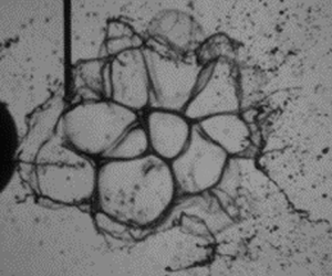
The end-on-view images show that at some point a rim forms around the periphery of the disk and draws the centre of the disk into a thinning sheet. This thinning sheet is more susceptible to the air flow and is the part of the drop that blows out into bags. At higher  $We$, such as in BS, MB and ST morphologies, the rim forms before all of the droplet has deformed and an undeformed core remains at the centre of the thinned membrane. The rim, sheet and undeformed core are highlighted in figure 6. From the present experiments, it is proposed that the breakup phase actually begins at the instant that the rim forms, as this signifies the transition of the governing mechanisms from the uniform expansion of the windward disk to the thinning and blowout of the interior that becomes the bag. This rim formation and undeformed core are also apparent in the numerical simulations of Jain et al. (Reference Jain, Prakash, Tomar and Ravikrishna2015), which show thickness modulations in the droplet profile at these locations.

Figure 6. Images of the structures formed at the end of the initiation period for BS (a) and MB (b) morphologies, showing the rolled rim (1), thinned sheet (2) and core (3).
If no undeformed core remains when the rim forms, the initiated structure comprises only of the rim and sheet. Since the sheet is only restricted at its periphery, it forms a single large bag when blown downstream. This condition describes Bag breakup and is shown in supplementary movies 1 and 2 available at https://doi.org/10.1017/jfm.2021.7 and in figure 7. At higher  $We$, the rim forms earlier in the deformation and the sheet is blown out while an undeformed core of the droplet remains. As
  $We$ increases, so does the amount of the drop that remains in the undeformed core. The undeformed core, like the rim, is less susceptible to forces of the air flow and the sheet is blown out between the undeformed core and the rim.

Figure 7. (a) Bag breakup sequence from side- (top) and end-on (bottom) views. See movie 1 (side view) and movie 2 (end-on view). (b) Illustration of droplet geometry at  $T_i$ (left) and of breakup morphology (right) for bag breakup. The windward disk is composed of the cross-hatched rim and the white area.
When the undeformed core is relatively small, the sheet forms a large bag that is pinched at its centre, which draws out the undeformed core to form the stamen. It is possible that during the formation of the stamen, air bubbles may be trapped as the navel of the bag pinches closed behind the stamen. The stamen size grows as the volume of the undeformed core increases with  $We$. The resulting breakup morphology in this case is BS and is shown in movies 3 and 4 and in figure 8. Similar thickness modulations are also seen in the numerical simulations of Yang et al. (Reference Yang, Jia, Che, Sun and Wang2017).

Figure 8. (a) BS breakup sequence from side (top) and end-on (bottom) views. See movie 3 (side view) and movie 4 (end-on view). (b) Illustration of droplet geometry at  $T_i$ (left) and of breakup morphology (right) for BS breakup. The windward disk is composed of the cross-hatched rim and the white area, while the undeformed core is marked by the grey-filled area.
Near the transition of Bag and BS breakup, evidence of a very small undeformed core can be seen that only mildly affects the growth of the bag and can form a slight dimple at the pole rather than a full stamen (figure 9). This shows the continuous nature of the transition between the Bag and BS breakup morphologies and how the stamen size changes with  $We$. This suggests that the topography of the bag thickness depends on the initiated structure with radial modulations in thickness. This is important in modelling the breakup of the bag as it is assumed to break first at its thinnest point. By comparison, current models assume a uniform thickness or that the bag is thinnest at its centre.

Figure 9. Side view showing the dimple formed at the tip of the bag near the transition from Bag to BS breakup.
When the undeformed core is large, the distance between the core and rim is small relative to the circumference of the rim. Owing to surface tension, a symmetric curvature is preferred in the bags, and thus multiple bags form along the azimuthal direction of the sheet. Unlike in BS breakup, the undeformed core in this case is large enough to continue being deformed and can breakup further as either an additional single bag or as consecutive waves of multiple bags (movies 5–6 and 7–8 and figure 10(top) and (bottom), respectively). The formation of the first set of bags as well as these two outcomes are illustrated in figure 11. Since multiple bags are formed azimuthally and multiple sequences of the breakup occur, this condition leads to MB breakup. This repeated breakup of the periphery was also seen in the experiments and numerical simulations of Dorschner et al. (Reference Dorschner, Biasiori-Poulanges, Schmidmayer, El-Rabii and Colonius2020), who noted that this results in a periphery which appears to be ‘flapping’.

Figure 10. (a) End-on and (b) side-view images of MB breakup showing the condition at which the remaining core breaks into one bag (top), and by repeated MB (bottom). See movies 5 and 6 (core breakup as single bag, side and end-on view, respectively), and movies 7 and 8 (core breakup as multiple bags, side and end-on view, respectively).

Figure 11. Illustration of MB bag formations, showing (a) the initiation and blowout of the first bag set, (b) the initiation and blowout of the core as a single bag, which occurs at lower  $We$, and (c) the initiation and blowout of a second bag set from the core along with the blowout of the core itself as the final bag. In (a), the windward disk is composed of the cross-hatched rim and the white area, while the undeformed core is marked by the grey-filled area.
Near the transition of BS and MB, the remaining core may be too small to break further, but the width of the thinned sheet relative to its radius may be enough to form multiple bags, usually two, as shown in figure 12. Some have referred to this as a distinct morphology called ‘twin-bag’, while others have grouped it either with BS or MB morphologies. The explanation of these breakup modes by the surface instability theory does not capture this ‘twin-bag’ behaviour, as the two stable wavelengths required for BS would also be required for two bags to form (i.e. it predicts the morphologies to be identical). The explanation provided here allows for the existence of the ‘twin-bags’ as a subset of MB in which the remaining core does not break further and multiple bags (two) form azimuthally.

Figure 12. Images showing the twin-bag structure at side (a) and end-on (b) views.
At higher  $We$, the aerodynamic forces of the air stream are dominant over the radial flow of the droplet. When this occurs, the rim is pushed downstream around the leeward face of the drop with a thin sheet that connects it to the undeformed core. The thin sheet is susceptible to the low-pressure zone at the periphery of the drop and is blown out radially with multiple bags formed azimuthally. This is shown in movies 9 and 10 and in figure 13. The remaining core then breaks as MB which is consistent with the numerical simulations of Dorschner et al. (Reference Dorschner, Biasiori-Poulanges, Schmidmayer, El-Rabii and Colonius2020). This breakup geometry resembles ST breakup, in that the periphery of the drop is drafted downstream. However, the present images show that instead of small droplets being stripped directly from the periphery of the drop, bag and rim structures are formed similar to the other breakup morphologies. Although the peripheral sheet has been observed in the numerical simulations of Jain et al. (Reference Jain, Prakash, Tomar and Ravikrishna2015) and Meng & Colonius (Reference Meng and Colonius2018), it is likely that this was not evident in previous experiments as the exposures required to capture the fast-moving structures is very short and the frame rate required to capture the radial blowout event is very high. These settings were only easily achieved with the present experimental set-up due to the ability to frame the video tightly to the droplet throughout the breakup. Additionally, the radial bag formation has likely not been seen in simulations due to mesh-induced breakup, which would prematurely ‘burst’ the bags before they are able to grow radially.

Figure 13. Sequential images showing the radial bag blowout that occurs in the ST morphology with side (a) and end-on (b) views.  $T$ gives the time of the first frame, while
  ${\rm \Delta} T$ gives the incremental time between each frame. Time moves forward from left to right. Note that the end-on view is at a lower frame rate, which was required in order to capture the necessary field of view. See movie 9 (side view) and movie 10 (end on).
Figure 14 shows illustrations of the structures of the droplet at initiation ( $T_i$) and their related breakup morphologies. These results highlight the importance of the geometry of the droplet during its deformation in determining the breakup morphology. Furthermore, the rims that form hold most of the droplet's volume during the breakup, thus modelling the rim dimensions at breakup is integral to determining the resultant breakup sizes of the drop. This is true even for cases with an undeformed core, as the core continues to deform and forms additional rim-bag structures until it is fully disintegrated.

Figure 14. Illustration of droplet at  $T_i$ (left) and of breakup morphology (right) for (a) Bag, (b) BS, (c) MB and (d) ST morphologies. The rim is marked by cross-hatching while the undeformed core is marked by the grey-filled area. The initiation disk is composed of the rim and the white area.
Since the simple ellipsoidal geometry that is assumed in previous analyses does not capture the rim, sheet and undeformed core features, these analyses cannot be expected to accurately model the transition between droplet deformation and breakup. Consequently, these models would have limited ability to predict breakup morphology and child droplet size. It is therefore necessary to develop a model which describes the formation of these structures, capturing the dimensions of the windward disk and of the rim at the instant of its formation which can be used to determine the volume that remains in the undeformed core. These geometries can then be used to determine the breakup sizes of the droplet and the breakup morphology.
4. Modelling droplet deformation and breakup
The windward disk from which the rim forms is the result of liquid flowing from the windward pole of the drop to its equator during the initiation period. The stable thickness of this disk balances the air pressure outside the droplet and the dynamic pressure inside the droplet, which results from the disk's constant deformation rate, via the Laplace pressure jump across the periphery. When the deformation persists past this point, the periphery of the windward disk forms a rim of the same thickness while the inner portion of the disk thins. The relationship between the windward disk and undeformed core volumes at this point dictates the breakup morphology. After this initiation period, the breakup period begins as the thinned portion of the windward disk is blown into one or more bags depending on the morphology, causing the rim to radially expand and thin until the bag ruptures which sets off the breakup of the rim. A flowchart of this modelling methodology is given in figure 15.

Figure 15. Flowchart of the present modelling methodology.
Thus, the first aim is to model the internal flow of the droplet, forced by the air flow around it, to determine the constant deformation rate. The constant deformation rate will then be used to determine the rim thickness at its formation and, by extension, the breakup morphology. Finally, the growth and breakup of the bag and rim will be modelled to predict the average child droplet sizes from the breakup of the rims, which contain the majority of the droplet volume.
4.1. Internal flow
The modelling of the internal droplet flow first carried out by Villermaux & Bossa (Reference Villermaux and Bossa2009) is replicated in this section for completeness of the present analysis. However, no assumptions about the shape of the droplet will be made that constrain the surface curvatures in the present section as to allow for greater generality of the resulting equation. These assumptions will be left to later sections. The coordinate system used in the present analysis is illustrated in figure 16(a).

Figure 16. Illustrations of (a) the coordinate system of the present analysis, (b) the actual droplet shape during the balancing period and (c) the approximated ellipsoidal geometry during the balancing period.
The liquid flow field inside the drop is found using the Navier–Stokes and conservation of mass equations in cylindrical coordinates for incompressible, axisymmetric radial flow,
 \begin{gather} \rho_{l}\left(\frac{\partial u_{r}}{\partial t}+u_{r} \frac{\partial u_{r}}{\partial r}\right)={-}\frac{\partial p_{l}}{\partial r}+\mu_l\left[\frac{1}{r} \frac{\partial}{\partial r}\left(r \frac{\partial u_{r}}{\partial r}\right)-\frac{u_{r}}{r^{2}}\right], \end{gather}
 \begin{gather}r \frac{\partial h}{\partial t}+\frac{\partial\left(r u_{r} h\right)}{\partial r}=0, \end{gather}
where  $p_l(r)$ is the radial pressure distribution inside the drop and
  $h = h(t)$ is the SW thickness of the drop as it flattens.
Defining the droplet's CS radius as  $R=R(t)$ and assuming that its volume is proportional to
  $R^2h$ (true for either ellipsoidal or cylindrical geometries), (4.2) gives the radial velocity profile inside the drop as
  $u_r(r)=r\dot {R}/R$. Upon substitution into (4.1), the viscous terms cancel. Integrating over
  $R$ leads to (4.3).
 \begin{equation} R\ddot{R} = \frac{2}{\rho_l}\left(p_l(0) - p_l(R)\right). \end{equation}
 The liquid pressure inside the drop is related to the surrounding air pressure by the Laplace pressure at the interface and is given by (4.4) where  $\sigma$ is the interfacial surface tension and
  $\kappa$ is the local surface curvature.
 \begin{equation} p_l(r)=p_g(r)+\sigma \kappa. \end{equation}
 The air-flow field is approximated as an inviscid stagnation-point flow against a plane at the windward pole of the drop with the axial component of the air velocity given by  $U_z=-a z U/d_0$, where
  $U$ is the free-field air-flow speed,
  $z$ is the axial direction measured from the windward pole of the droplet and
  $a$ is the stretching rate of the air flow (i.e. the spacing between the streamlines of the flow). Here,
  $a$ essentially relaxes the planar stagnation-point flow assumption to approximate the windward droplet face topology. The limiting shapes of the deformation process are the initial sphere and a final disk, which correspond to
  $a=6$ and
  ${\rm \pi} /4$, respectively (Villermaux & Bossa Reference Villermaux and Bossa2009). The pressure field in
  $r$ and
  $z$ of the surrounding air flow is found by conservation of mass and momentum assuming inviscid, incompressible, quasi-steady and axisymmetric flow, which is solved at
  $z=0$ to find the pressure at the windward face of the drop given by (4.5).
 \begin{equation} p_{g}(r)=p_{g}(0)-\rho_{g} \frac{a^{2} U^{2}}{8 d_{0}^{2}} r^{2}. \end{equation}
Substituting (4.4) and (4.5) into (4.3) and non-dimensionalizing gives
 \begin{equation} \frac{\ddot{R}}{R}=\frac{1}{\tau^2}\left(\frac{a}{2}\right)^2 \left[1-\frac{8}{a^2We}\frac{(\kappa_p - \kappa_w)d_0^3}{R^2}\right], \end{equation}
where  $\kappa _p$ and
  $\kappa _w$ are the curvatures at the periphery and windward pole of the drop, respectively. It is clear from (4.6) that the deformation rate of the droplet depends on its shape as it deforms as the aerodynamic forces depend on the stretching rate while the surface tension forces depend upon the curvature at the windward face and periphery of the drop, all of which change as the droplet deforms. In order to avoid the cyclical argument that to solve the deformation of the droplet one must know the deformation of the droplet, assumptions must be made to describe the droplet's shape during the deformation to determine the values of
  $\kappa _p$,
  $\kappa _w$ and
  $a$.
$a$.
Equation (4.6) is the most general form of the model for the internal liquid flow of a droplet in a high-speed air stream. Similar approaches have been taken by Villermaux & Bossa (Reference Villermaux and Bossa2009) and Kulkarni & Sojka (Reference Kulkarni and Sojka2014), however, these attempts did not predict the constant radial growth rate that is found here. These analyses are discussed further in appendix C.
4.2. Droplet deformation
Using the equations for the internal flow of the droplet, the problem now turns to determining the constant radial growth rate that is observed during the initiation period of the breakup.
Upon inspection of (4.6), a constant radial growth rate would occur when the term in square brackets becomes zero, i.e. the aerodynamic and surface tension forces balance. This is expected as the deformation causes the droplet's windward face to flatten, thus  $a$ decreases from
  $6$ towards
  ${\rm \pi} /4$ while
  $\kappa _w$ tends towards zero as the windward face flattens and
  $\kappa _p$ increases as the periphery thins, as illustrated in figure 16(b). This process is described as ‘flow balancing’ as the forces acting on the droplet change through the deformation until they balance resulting in the constant growth rate (
 $\ddot {R}=0$). This description is consistent with the division of the deformation stage into two periods; the initial windward pole flattening period and the constant radial expansion period as described in § 3.
The constant radial expansion rate is achieved once the flows have balanced, which occurs at the flow balancing time,  $T_{bal}$. Since the radial flow near the pole at early
  $T$ does not greatly affect the flow at the periphery of the drop where the CS deformation measurement is taken,
  $T_{bal}$ is defined by the point at which the SW deformation becomes approximately constant. From the present experiments,
  $T_{bal}\approx 1/8$ appears to be a good estimate as shown in figure 17 where the constant SW deformation rate begins at
  $T\approx 1/8$. In other words,
  $T_{bal}$ is taken as the time at which the disk first begins to form on the windward face of the drop.

Figure 17. (a) CS and SW droplet deformation  $L/d_0$ vs. time
  $T$ for
  $We = 9.6$ (Bag) and
  $We = 22.5$ (BS) over the initiation period. (b) Magnification of the region given by the box in (a). The constant SW deformation rate occurs at
  $T_{bal} \approx 1/8$ for both cases, indicated by the vertical dashed line.
Initially, the droplet is spherical, therefore  $\kappa _w = \kappa _p$ and the surface tension terms cancel. However, as the windward face flattens,
  $\kappa _w$ rapidly diminishes and becomes negligible. The curvature of the periphery is composed of two curvatures: the thickness curvature,
  $\kappa _{h}=2/h$, and the azimuthal curvature,
  $\kappa _{\theta }=1/R$. In previous analyses,
  $\kappa _{\theta }$ was neglected as it was assumed to be much smaller than
  $\kappa _{h}$ (see appendix C). However, this is not the case for the levels of deformation that occur up to
  $T_{i}$ where
  $2R/d_0 < 1.6$, as shown in figure 18 where the ratio between the curvatures is less than an order of magnitude for deformations less than
  $2R/d_0 \approx 2$. This is likely a significant reason that 2-D numerical simulations, which neglect this curvature, perform poorly compared to their 3-D equivalents (Strotos et al. Reference Strotos, Malgarinos, Nikolopoulos and Gavaises2016). In figure 18,
  $h/d_0$ is found by conservation of mass for both ellipsoidal and cylindrical geometries (
 $h/d_0 = (d_0/2R)^2$ and
  $h/d_0 = 2/3(d_0/2R)^2$, respectively). The azimuthal curvature therefore cannot be neglected in the analysis of the droplet deformation for
  $T<T_{i}$, including over
  $T_{bal}$.

Figure 18. Ratio of the thickness curvature to the azimuthal curvature vs. extent of deformation for ellipsoid and disk geometries ( $h/d_0 = (d_0/2R)^2$ and
  $h/d_0 = 2/3(d_0/2R)^2$, respectively).
Equation (4.6) is then,
 \begin{equation} \frac{\ddot{R}}{R}=\frac{1}{\tau^2}\left(\frac{a}{2}\right)^2\left[1-\frac{64}{a^2We} \left( \left(\frac{d_0}{h}\right) \left(\frac{d_0}{2R}\right)^2 +\left(\frac{d_0}{2R}\right)^3 \right)\right]. \end{equation}
 To finalize the definition of the curvatures, an assumption must be made about the geometry of the droplet during the flow balancing such that  $h$ and
  $R$ can be related. It is assumed that during the flow balancing period the droplet can be approximated by an ellipsoid as illustrated in figure 16(c) such that, by conservation of mass with the initially spherical droplet,
  $h/d_0 = (d_0/2R)^2$ (this assumption is discussed further in appendix C). This simplifies (4.7) to 4.8, where the only remaining unknown is
  $a$
$a$
 \begin{equation} \frac{\ddot{R}}{R}=\frac{1}{\tau^2}\left(\frac{a}{2}\right)^2\left[1-\frac{64}{a^2We} \left( 1 +\left(\frac{d_0}{2R}\right)^3 \right)\right], \end{equation}
where  $a$ relates to the approximation of the flow around the deforming object as a planar stagnation-point flow. While its limits are defined as
  $a=6$ for the initial sphere and
  $a={\rm \pi} /4$ for a disk, the relationship between
  $a$ and the extent of deformation (i.e. the path of
  $a$ from
  $6$ to
  ${\rm \pi} /4$) is unknown. While it is possible that a relationship between
  $a$ and the shape of the droplet could be determined from numerical simulation or by highly detailed particle image velocimetry (PIV) measurements, it will be assumed that the dominant value of
  $a$ over the deformation period is its initial value as this results in the highest
  $\ddot {R}$ during the balancing period. Additionally, it is observed that the shape of the droplet as a whole is more spherical than disk like during the balancing period. Thus, over the balancing period, it is assumed that
  $a$ takes a constant value of
  $a=6$. The constant radial expansion rate is then found by integrating (4.8) over the flow balancing time. As described earlier in this section, the CS dimension of the drop remains roughly constant during the flow balancing, thus
  $R(T<T_{bal}) \approx d_0/2$. This integration leads to (4.9)
 \begin{equation} \frac{\dot{R}}{d_0/2} = \frac{1}{\tau}\left(\frac{a}{2}\right)^2\left(1-\frac{128}{a^2We}\right) T_{bal}. \end{equation}
 The prediction of (4.9) is compared to the experiments in figure 19, where the constant radial growth rate is measured by performing a linear fit to the cross-sectional diameter measurements over the period  $0.25<T<T_{i}$ for all cases. Good agreement between the theory and experiments is found for Bag and BS breakup morphologies (figure 19b). MB and ST morphologies exhibit greater deviation due to the early breakup as described in § 3, in particular the breakup of the liquid fragment at the top of the drop which results from the suspending needle which becomes the windward most point of the drop which affects the measurement as in § 2. This has a greater effect on the fitting procedure as there are fewer data points during the deformation phase which are undisturbed owing to the faster progression of the deformation relative to the frame rate used.

Figure 19. Comparison of predicted expansion rate from (4.9) to all experiments (a) and to NB, Bag and BS morphologies only (b). The box in (a) shows the region that is magnified in (b).
Figure 20 compares the present deformation prediction as well as the previous deformation models (the TAB model of O'Rourke & Amsden (Reference O'Rourke and Amsden1987) and the models of Villermaux & Bossa Reference Villermaux and Bossa2009; Kulkarni & Sojka Reference Kulkarni and Sojka2014) to the present experiments for a range of  $We$ covering Bag and BS morphologies. Note that the present model does not rely on exactly predicting the temporal deformation and instead focuses only on predicting the constant deformation rate. As such, for figure 20, the present model is plotted assuming that the CS expansion first passes the periphery of the drop at
  $T \approx 0.25$, with the slope given by (4.9). Excellent prediction of the present model is shown, while the previous models show significant deviation and indeed a misrepresentation of the constant trend.

Figure 20. Comparison of TAB (O'Rourke & Amsden Reference O'Rourke and Amsden1987), Villermaux & Bossa (Reference Villermaux and Bossa2009) and Kulkarni & Sojka (Reference Kulkarni and Sojka2014) models and (4.9) to the CS measurement of the present experiments during initial deformation.
The present prediction also agrees with the numerical results of Jain et al. (Reference Jain, Tyagi, Prakash, Ravikrishna and Tomar2018), who studied the effect of density ratio,  $\rho ^{\ast }=\rho _l/\rho _g$, on the breakup. In their work,
  $\dot {R}(T=1)=4.8$,
  $2.0$ and
  $0.8$ for
  $\rho ^{\ast } = 10$,
  $150$, and
  $1000$, respectively, at
  $We=20$. The corresponding values using the present analysis are
  $\dot {R}(T=1)=5.9$,
  $1.5$, and
  $0.6$. The prediction of the present analysis is higher than that of Jain et al. (Reference Jain, Tyagi, Prakash, Ravikrishna and Tomar2018) at
  $\rho ^{\ast }=10$ as the resistance due to the gas phase density on the expanding periphery is not accounted for. The present prediction is lower for the other cases as the measurements of Jain et al. (Reference Jain, Tyagi, Prakash, Ravikrishna and Tomar2018) are taken after
  $T_i$ (
 $T_i<1$), when the flow dynamics begins to change, as will be described in § 4.4. Chou & Faeth (Reference Chou and Faeth1998) empirically found the growth rate to be
  $2 \dot {R} / d_0 = 1.06$ and
  $1.22$ for their water experiments at
  $We=13$ and
  $20$, respectively (
 $2\dot {R} / d_0\tau = 0.5$, with
  $\tau =0.472$ and
  $0.41$ ms for
  $We=13$ and
  $20$, respectively). This result is low compared to the present predictions of
  $1.8$ and
  $2.26$; however, several high-viscosity cases were included in the results of Chou & Faeth (Reference Chou and Faeth1998). Adjusting their analysis for their water experiments only gives
  $2\dot {R}/d_0=1.31$ and
  $1.95$. These results agree relatively well with those of the present study considering the much lower time resolution of Chou & Faeth (Reference Chou and Faeth1998), which may cause a higher uncertainty in the linear fit.
4.3. Rim formation and prediction of initiation geometry
The majority of the child droplets that form from the breakup of the drops come from the rim geometries described in § 3. Furthermore, the rim size can be used to find the initiation geometry in order to determine the breakup morphology. It is therefore necessary to predict the rim size when it forms, which can be found by solving for the internal flow inside the windward disk.
As the droplet's windward face expands radially, the disk that forms has thickness  $h$. At the instant of initiation, the periphery of the disk ‘rolls’ as the surface tension pinches the sides of the disk periphery to form a thick rim of major and minor diameters
  $2R_i/d_0$ and
  $d_{i} \approx h_i$, respectively. This geometry is illustrated for all breakup morphologies in figure 21. The pressure balance across the peripheral interface (4.4) can be used to find
  $h_i$, giving (4.10)
 \begin{equation} d_{i} = h_{i} =\left[\frac{1}{4 \sigma}\left(\rho_{l} \dot{R}^{2}+\rho_{a} \left(\frac{a}{2}\right)^{2} U^2\left(\frac{R_i}{d_{0}}\right)^{2}\right)-\frac{1}{2 R_i}\right]^{{-}1}. \end{equation}
Figure 21. Illustration of the (a) initial droplet and the deformed droplet geometry at  $T_i$ for (b) Bag, (c) BS, (d) MB and ST morphologies, indicating measurement locations of
  $h_i$ and
  $R_i$. The rim is marked by cross-hatching while the undeformed core is marked by grey fill.
While  $2R_i/d_0$ and
  $h_i$ both serve to balance the pressure across the interface, one must be known in order to uniquely determine the other. At this time, the mechanism which determines the unique values is unknown, therefore, an assumption will be made for
  $2R_i/d_0$ based on the present experiments so that
  $h_i$ may be determined. Figure 22(a) shows the measured CS diameter of the droplets at
  $T_{i}$, which for all breakup modes is determined from the average of the Bag and BS morphologies as
  $2R_{i}/d_0 \approx 1.6$. This value agrees with the breakup criterion for the TAB model,
  $2R/d_0 =1.5$, as well as the experimental findings of Zhao et al. (Reference Zhao, Liu, Cao, Li and Xu2011a),
  $2R/d_0 =1.8$, who used the older definition of
  $T_i$ that is slightly later than the definition presently used, resulting in a slightly higher value as discussed in § 3.

Figure 22. Measurements of droplet periphery thickness (a) and diameter (b) at  $T_{i}$. Periphery thickness measurement is compared to the present model (4.11). Droplet CS diameter reaches a value of
  $2R_{i}/d_0 \approx 1.6$ for all breakup modes.
In this late stage of deformation,  $a$ will satisfy the balancing of (4.3) for the initiated geometry and is found to be
  $a \approx \sqrt {80/We}$. This suggests a shift in dominance of the aerodynamic forces over the inertia of the expanding rim when
  $We > 80$, which coincides with the transition to the ST morphology as described by Guildenbecher et al. (Reference Guildenbecher, López-Rivera and Sojka2009). This then gives that
  $We_{c,ST}=80$, which agrees with the present experiments as well as with Guildenbecher et al. (Reference Guildenbecher, López-Rivera and Sojka2009) and Zhao et al. (Reference Zhao, Liu, Li and Xu2010). Using these assumptions, (4.10) simplifies to
 \begin{equation} \frac{d_{i}}{d_0} = \frac{h_{i}}{d_0} \approx \left[\frac{1}{4} \left( \frac{\rho_l \dot{R}^2 d_0}{\sigma} \right) + 2.6 \right]^{{-}1} = \frac{4}{\left(We_{rim}+10.4\right)}, \end{equation}
where the term  $\rho _l \dot {R}^2 d_0 / \sigma$ is grouped as a ‘rim Weber number’,
  $We_{rim}$, which describes the competition between the radial momentum induced at the droplet periphery and the restoring surface tension of the stable droplet. For
  $We_{rim} < 1$, the radial flow momentum is not strong enough to significantly overcome surface tension and the drop will oscillate with NB occurring. However, for
  $We_{rim}>1$, the radial momentum of the drop's periphery is great enough to overcome this restoring force, allowing the periphery to continuously extend, facilitating the thinning and blowout of the interior. This criticality defines the onset of the Bag morphology, where
  $We_{rim}=1$ and (4.9) lead to
  $We_{c,Bag}\approx 8.8$, which agrees well with the present experiments, as shown in figure 23(a), and to the previous results discussed in § 1. Since the derivation of (4.11) does not account for any slowing in
  $\dot {R}$, which results from the thinning periphery, the present prediction is slightly high near
  $We_{c,Bag}$ where
  $We_{rim}$ is low.

Figure 23. Measurements of  $We_{rim}$ vs.
  $We$ (a) and periphery thickness vs.
  $We_{rim}$ (b) compared to the prediction of (4.11). The criticality
  $We_{rim}=1$ agrees with the transition to the Bag morphology and defines
  $We_{c,Bag}\approx 8.8$ (a), and periphery thickness vs.
  $We_{rim}$ compared to the prediction of (4.11) (b).
The prediction of (4.11) is compared to the experiments with  $We$ and
  $We_{rim}$ in figures 22(b) and 23(b), respectively. The measurements shown in these figures are taken at the periphery of the droplet in order to measure the thickness of the rim, as measurements taken across the centre of the drop result in larger values due to the undeformed core. Examples of this measurement are shown in figure 24. Although the trend agrees well with the experiments, the prediction of (4.11) consistently over-predicts the measurements by
  $\approx 0.05$ (note that a conservative measurement error of
  $\pm$1 pixel results in
  ${\pm }0.025$). A possible cause of this overprediction is that the present analysis neglects flow separation around the periphery of the windward disk. Flow separation would cause a lower pressure at the periphery than is presently modelled, especially near
  $T_i$ when the windward disk is at its thinnest. This affects the balance of the surface tension and pressure terms that govern the rim's formation and would cause it to be thinner than predicted.

Figure 24. Example of  $h_i$ measurement from droplet periphery for low (a) and high (b)
  $We$.
$We$.
With a good prediction of the dimensions of the initiation geometry, the core volume can be determined and used to predict the initiation geometry. The windward disk is modelled as a flat disk with rounded edges having a radius of  $R_i$ and a thickness of
  $h_i$ (i.e. the intersection of a short cylinder and a torus). The leading coefficient of the
  $h_i^3$ term in the volume equation for this geometry is very small compared to the other coefficients and can therefore be neglected. The volume of the disk,
  $V_d$, is thus given by (4.12). The undeformed core is then the volume that remains from the initially spherical droplet (
 $V_0 = 4/3 {\rm \pi}(d_0/2)^3$), given by
  $V_{c}=V_{0}-V_{d}$ (4.13)
 \begin{gather} \frac{V_{d}}{V_0} = \frac{3}{2} \left[ \left(\frac{2R_i}{d_0}\right)^2 \left(\frac{h_i}{d_0}\right) - 2 \left(1-\frac{\rm \pi}{4}\right) \left(\frac{2R_i}{d_0}\right) \left(\frac{h_i}{d_0}\right)^2 \right] \end{gather}
 \begin{gather}\frac{V_{c}}{V_0} = 1 - \frac{3}{2} \left[ \left(\frac{2R_i}{d_0}\right)^2 \left(\frac{h_i}{d_0}\right) - 2 \left(1-\frac{\rm \pi}{4}\right) \left(\frac{2R_i}{d_0}\right) \left(\frac{h_i}{d_0}\right)^2 \right]. \end{gather}
 Figure 25 plots  $V_d$ (a) and
  $V_c$ (b) for the present experiments with the predictions. As with the prediction of
  $d_{i}$ (4.11), the trend matches well; however,
  $V_d$ is slightly overpredicted resulting in the underprediction of
  $V_c$, delivering nonsensical results such as
  $V_d > V_0$ for low
  $We$. The over/underprediction of these volumes is the consequence of the overprediction of
  $d_{i}$, therefore, to improve the model for the volume distribution at initiation, the prediction of
  $d_{i}$ must be further improved. However, the experimental results can still be used to define the criterion for the transition between the various breakup morphologies. These trends also agree reasonably well with the experimental results of Dai & Faeth (Reference Dai and Faeth2001), considering the potential errors of their measurement method (i.e. measuring the volume of the drops after the breakup, as well as relatively low spatial resolution).


For Bag breakup, it is expected that there is no undeformed core, therefore this morphology will occur when  $V_d/V_0 \approx 1$ (
 $V_c/V_0 \approx 0$), which matches the experiments as indicated by the dashed line in figure 25.
As described in § 3, BS, MB and ST morphologies occur when  $V_c/V_0 > 0$ (
 $V_d/V_0 < 1$), however, the criterion for
  $V_c/V_0$ required for the transition from BS to MB is not as obvious as the transition from Bag to BS. From figure 25 it can be seen that this transition occurs at
  $V_c/V_0 \approx 0.5$ (indicated by the dash-dotted line), i.e. exactly half of the drop is undeformed. The mass per unit frontal surface area of the undeformed core is maximal at this point (assuming it takes roughly the shape of a spherical cap). This gives the core the greatest resistance to being pushed downstream by the air flow and allows the sheet to be blown out before the core deforms significantly. This explanation agrees with the physical description of the MB breakup process in § 3.
The transition to ST from MB is governed by the aerodynamic forces and not  $V_c$, therefore there is no expected insight into the ST transition from this volume-based analysis.
With this rough prediction of the breakup morphology and of the rim dimensions at initiation, a prediction for the child drop sizes which result from the breakup of the rim can now be formulated.
4.4. Rim expansion and bag blowout
The breakup sizes from the rim will be proportional to its diameter at breakup. It is therefore necessary to find the rim diameter after it has grown to the breakup size. From conservation of mass on the rim, which formed at  $T_{i}$ with an initial minor and major diameter (
 $d_{i}$, and
  $2R_i$, respectively) and the final rim minor and major diameter (
 $d_{f}$ and
  $2R_f$),
  $d_{f}$ is found by (4.14)
 \begin{equation} d_{f} = d_{i} \sqrt{\frac{R_i}{R_f}} \end{equation}
 Since the initiation geometry,  $R_i$ and
  $d_{i}$, have already been defined in § 4.3, the remaining factor to be determined is
  $R_f$, i.e. the extent of the rim's expansion. The formation of the rim coincides with the formation of the sheet between the rim and the undeformed core which becomes the bag structures after
  $T_{i}$. The initial stage of the rim's growth continues at the constant
  $\dot {R}$ found by (4.9). During this stage, the bag size,
  $\beta$, is smaller in the SW direction than in the CS. Once the bag grows to and past the size of the rim, it pulls on the rim and accelerates its growth until the bag breaks, after which the rim continues to grow at a constant rate. This is seen in figure 5, and the geometries of interest are illustrated in figure 26.

Figure 26. Illustration of droplet geometry at (a)  $T_0$, (b)
  $T_i$, (c)
  $T_i^+$ and (d)
  $T_f$ for bag breakup with the relevant dimensions for the rim expansion and bag growth indicated. The rim is marked by cross-hatching, while the remainder of the windward disk is marked by the white area.
When the bag eventually ruptures, it quickly recedes around the bag (as described by Lhuissier & Villermaux Reference Lhuissier and Villermaux2012) and collides with the droplet's rim, instigating its breakup. Therefore, it is assumed that the final size of the rim is proportional to the final size of the bag when it breaks. In the cases of BS and MB breakup, the bag is confined further by the undeformed core. By determining the bag size at burst,  $\beta _f$, one can approximate
  $R_f$ and thus determine the child drop size,
  $d_c$. Vledouts et al. (Reference Vledouts, Quinard, Vandenberghe and Villermaux2016) modelled the breakup of accelerating liquid shells by supposing that the interface is susceptible to the Rayleigh–Taylor instability with a growth rate,
  $\omega$, given by (4.15),
 \begin{equation} \omega(t^{{\ast}})=\sqrt{\frac{\rho_l \ddot{\beta}^{2}(t^{{\ast}}) h(t^{{\ast}})}{2 \sigma}}, \end{equation}
where  $\beta (t^{\ast })$ is the SW dimension of the bag and
  $h(t^{\ast })$ is the membrane thickness at time
  $t^{\ast }=t-t_i$, as illustrated in figure 26(c). The breakup time was estimated by (4.16) where
  $C$ is a constant of
  $O(1)$
 \begin{equation} \int_{0}^{t^{{\ast}}_{b}} \omega(t^{{\ast}}) \,\mathrm{d} t^{{\ast}} = C. \end{equation}
Performing a force balance on the tip of the bag as in Villermaux & Bossa (Reference Villermaux and Bossa2009), the bag tip acceleration is found as
 \begin{equation} \ddot{\beta}(t^{{\ast}})=\frac{p_0}{\rho_l h(t^{{\ast}})}. \end{equation}
 Although Kulkarni & Sojka (Reference Kulkarni and Sojka2014) included surface tension in the force balance, its effect is negligible. At its largest value (when the bag size is the size of the rim), it effectively lowers the pressure by  $\sigma /2 << p_0$ for all cases.
The value of  $h(t^{\ast })$ is determined by conservation of mass of the expanding disk, approximating it as a cylinder of radius
  $R-h_i$ and thickness
  $h$, giving
  $h(t^{\ast })\approx V_b / {\rm \pi}(R-h_{i})^{2}$ where
  $V_b$ is the volume of the bag. The volume of the bag is the volume of the windward disk that is not in the rim (
 $V_b = V_d - V_r$).
  $V_d$ was given earlier by (4.12). The rim is modelled as a torus of major and minor diameters
  $2R_i$ and
  $h_i$, with
  $V_r$ given by (4.18). It is worthwhile to note that for the Bag morphology, (4.18) estimates that the rim contains 50 %–80 % of the droplet volume which agrees with the findings of previous works (see appendix B), and is thus a good approximation of the droplet geometry. Since the disk expands at a constant rate, the radius can be estimated by
  $R=R_i + \dot {R}t^{\ast }$
 \begin{gather} \frac{V_{r}}{V_{0}}=\frac{3 {\rm \pi}}{2}\left[\left(\frac{2 R_i}{d_{0}}\right) \left(\frac{h_i}{d_{0}}\right)^{2}-\left(\frac{h_i}{d_{0}}\right)^{3}\right] \end{gather}
 \begin{gather}\frac{V_{b}}{V_{0}}=\frac{3}{2}\left[\left(\frac{2 R_i}{d_{0}}\right)^{2} \left(\frac{h_i}{d_{0}}\right)-\left(\frac{2 R_i}{d_{0}}\right)\left(\frac{h_i}{d_{0}}\right)^{2}\left(2+\frac{\rm \pi}{2}\right)+ {\rm \pi}\left(\frac{h_i}{d_{0}}\right)^{3}\right] \end{gather}
The breakup time,  $t^{\ast }_{b}$, is then found by substituting
  $h$ into (4.15) and performing the integral in (4.16), leading to (4.20) where the only term that remains to be determined in the constant
  $C$
$C$
 \begin{equation} t^{{\ast}}_{b}=\frac{\left[\left(\dfrac{2 R_{i}}{d_{0}}\right)- 2\left(\dfrac{h_{i}}{d_{0}}\right)\right]}{\left(\dfrac{2 \dot{R}}{d_{0}}\right)} \left[{-}1+\sqrt{1+C \frac{8 \tau}{\sqrt{3 W e}} \sqrt{\frac{V_{b}}{V_{0}}} \frac{\left(\dfrac{2 \dot{R}}{d_{0}}\right)}{\left[\left(\dfrac{2 R_{i}}{d_{0}}\right)-2 \left(\dfrac{h_{i}}{d_{0}}\right)\right]}}\right]. \end{equation}
 A much more detailed analysis of the instability growth in the bag is required in order to determine  $C$ analytically, however, the present data are not well suited for this as the instability cannot be resolved on the bag. To determine
  $C$, (4.20) is fit to the breakup time data of the present experiments and is found to be
  $C \approx 9.0$, as shown in figure 27(b). In Vledouts et al. (Reference Vledouts, Quinard, Vandenberghe and Villermaux2016), (4.16) was applied directly to an already thin shell where the instability grows for the entire duration of
  $t^{\ast }_b$, thus the breakup time is relatively short and
  $C=O(1)$. In the present analysis, the definition of
  $t^{\ast }_b$ to which (4.20) is fit includes the initial formation of the bag after
  $T_i$ when
  $\ddot {\beta }$ is small and
  $h$ is relatively large. In this case, the instability does not develop appreciably for much of
  $t^{\ast }_b$, and
  $C>O(1)$. The bag size at time
  $t^{\ast }$,
  $\beta (t^{\ast })$, is found by integrating (4.17) with the substitution of
  $h$, leading to (4.21)
 \begin{align} \frac{\beta\left(t^{*}\right)}{d_{0}} &= \frac{3}{4}\left(\frac{V_{0}}{V_{b}}\right) \frac{1}{\tau^{2}}\left\{\left[\left(\frac{2 R_{i}}{d_{0}}\right)-2 \left(\frac{h_{i}}{d_{0}}\right)\right]^{2} \frac{t^{* 2}}{2} \right. \nonumber\\ &\quad \left.+\left(\frac{2 \dot{R}}{d_{0}}\right) \left[\left(\frac{2 R_{i}}{d_{0}}\right)-2\left(\frac{h_{i}}{d_{0}}\right)\right] \frac{t^{* 3}}{3}+\left(\frac{2 \dot{R}}{d_{0}}\right)^{2} \frac{t^{* 4}}{12}\right\}. \end{align}


Solution of (4.21) at time  $t^{\ast }_{b}$ (4.20) gives the bag size at the time it ruptures,
  $\beta _f$, which is compared to the experiments in figure 27(b). Although the prediction of
  $\beta$ and
  $\beta _f$ match the experiments within the errors typical of these experiments (see appendix B), it is clear that the model does not capture all of the dynamics of the bag. In particular, the model underpredicts
  $\beta _f$ at the higher
  $We$ range of the BS morphology (
 $20 < We < 30$). It is likely that this is the result of the shape of the bag around the stamen. This shape causes the bag to be thicker between the stamen and the tip of the bag, thus the thinnest point of the bag is between the bag tip and the rim. This would result in a slightly longer breakup time, as the most susceptible point on the bag is farther away from the tip where the acceleration is expected to be the greatest.
Equation (4.21) evaluated over  $0<t^{\ast }<t^{\ast }_b$ is compared to experiments in figure 28, showing excellent agreement over a range of
  $We$ for each morphology, with the exception of the upper
  $We$ limit for MB (f). In this case, the SW measurement appears to grow faster than the prediction. At the high
  $We$ limit of the MB morphology, the ST mechanics which draw the periphery downstream begin to become significant. As a result, the rim is drawn somewhat downstream during this phase and dominates the SW measurement in the early stages of the bag growth, causing apparent disagreement between the present model and experiments. Even though this partial ST occurs, the breakup ultimately persists as in MB.

Figure 28. Experimental CS and SW droplet deformation  $L/d_0$ vs. time
  $T$ for various
  $We$ and morphologies (annotated in figure). Equation (4.21) is given by the solid black lines, where the solid black dots indicated the breakup point as calculated from (4.20). Every fourth data point is plotted for clarity.
The relationship between  $\beta _f$ and
  $2R_f$ depends on the morphology of the breakup. The breakup geometries are illustrated in figure 29, showing the assumed relationships between
  $\beta _f$ and
  $2R_f$. For Bag breakup, the bag is only constrained by the rim, and since in the late stage of the bag growth the bag size matches the rim diameter, the relationship
  $2R_f \approx \beta _f$ is suitable (a) (see figure 7). For BS, the stamen causes a central fold of the bag, thus
  $2R_f \approx 2\beta _f$ (b) (see figure 8). This is similar for the MB morphology, however, the undeformed core plays a more significant role, and
  $2R_f \approx d_0 + 2\beta _f$ (
 $c$) (see figures 10 and 11). Finally, for ST, the rim of the droplet is pulled downstream right after it forms at diameter
  $2R_i/d_0$ (d) (see figure 13). The ratio of
  $2R_f$ to
  $\beta _f$ is plotted for all morphologies in figure 30(a). Figure 30 generally agrees with the above assumptions, showing that for Bag breakup
  $2R_f/\beta _f \approx 1$ and for MB
  $2R_f/\beta _f > 2$, however, it is clear that there is a continuous transition between the Bag and BS morphologies which is not captured here. As with the prediction of
  $\beta _f$, this is expected to be the result of the thickness modulations which occur due to the Bundt cake shape of the bag in the BS morphology. The prediction of
  $2R_f$ is shown in figure 30(b). While the prediction generally agrees with the average of each morphology, it is again clear that a derivation which takes into account the effect of the continuity in the change of the core size as a result of the growing undeformed core on
  $2R_f/\beta _f$ will provide better agreement across the Bag and BS morphologies.

Figure 29. Illustration of the breakup geometry for (a) Bag, (b) BS, (c) MB and (d) ST morphologies. Measurements of and relationships between  $R_f$ and
  $\beta _f$ are indicated. The rim is marked by cross-hatching while the undeformed core is marked by grey fill.

Figure 30. (a) Rim vs. bag size at burst ( $2R_f/\beta _f$) for all breakup morphologies. The solid black line gives
  $2R_f/\beta _f = 1$ and the dashed black line gives
  $2R_f/\beta _f=2$, indicating the assumed value of
  $2R_f/\beta _f$ for Bag and BS morphologies, respectively. (b) Rim major diameter at burst (
 $2R_f/d_0$) with prediction of (4.14).
The prediction of the rim expansion ratio,  $R_i/R_f$, can now be substituted into (4.14), which is compared with the experiments in figure 31(a), showing good agreement with the results despite not fully capturing the continuous transitions as described previously.

Figure 31. Measured rim minor diameter (a) and rim-thinning ratio (b) vs.  $We$. Solid and open markers are for side and end-on experiments, respectively. Lines give the prediction of (4.14) (a) and the median rim-thinning ratio (b).
In the interest of formulating a continuous prediction, the median rim thinning ratio,  $d_r/d_i \approx 0.64$, is estimated from the experiments (figure 31b) to be used as a comparison in the next section. Note that the spread of the rim-thinning ratio in figure 31 is fairly large, thus this term will only be used as a rough estimation in order to assess the effects of the prior assumptions on the breakup prediction without the complexity of the morphology variation.
Chou & Faeth (Reference Chou and Faeth1998) performed a similar analysis using several simplifications. In their analysis, the growth of the rim was determined directly by performing the momentum balance between the rim and bag assuming the rim and bag thicknesses to be constant and the rim volume to be  $V_r/V_0=0.65$. This was then fit to their results using a coefficient analogous to
  $C_d$, which accounts for variations in the relationship of the stagnation pressure and rim expansion. The expansion was then related to the rim thinning by conservation of mass as was done in the present work, although the terminal rim size was determined empirically. The rim was also assumed to continue growing after the breakup of the bag, with bag and rim breakup times determined empirically. The rim breakup was modelled by Rayleigh–Plateau instability, as in § 4.5. Due to these simplifying assumptions, as well as a relatively small data set with which to fit, their work was not able to predict beyond the narrow range of
  $15<We<20$. Essentially, the work of the present section accounts for the variations in these assumptions, allowing it to achieve good prediction across a range of
  $We$ and morphologies.
4.5. Rim breakup
Confounding factors such as the number and location of the rupture sites and collisions of the rupture fronts with each other and with the main rim of the droplet are numerous (see, for example, figure 32). While many of these phenomena have been studied previously (Bremond & Villermaux Reference Bremond and Villermaux2005; Lhuissier & Villermaux Reference Lhuissier and Villermaux2012; Vledouts et al. Reference Vledouts, Quinard, Vandenberghe and Villermaux2016; Poulain, Villermaux & Bourouiba Reference Poulain, Villermaux and Bourouiba2018), predictions of when each mechanism will be preferred in the breakup are still illusive. The present experiments cannot be compared directly to these works due to the limitations of the high-speed camera. The bag breakup period occurs on a very short time scale ( $T < 0.2$) and at a very small spatial scale (
 $d_b$ of the order of
  $\mathrm {\mu }$m). Since it is not possible to achieve the desired time and spatial resolution while maintaining the wide field of view that is necessary to capture the entire breakup process, the present experiments are unable to provide insights into the breakup of the bags formed in droplet breakup.

Figure 32. Time-series images of the breakup of the bag showing (a) a single rupture and (b) multiple ruptures. Here,  $T$ gives the time of the first frame, while
  ${\rm \Delta} T$ gives the incremental time between each frame;
  $T$ increases from left to right and continues in the bottom row.
As mentioned previously, the rims that form in droplet breakup contain much more of the droplet's mass than the bags. Additionally, much of the volume of the bag merges with the rim of the droplet once the bag recedes. The result is that most of the droplet's volume ends up being part of the rim breakup process and the droplets formed from the bag are far less important in terms of volume than those formed by the rim. It is therefore of higher importance to model the breakup of the rim.
Once the bag has completed its breakup, the rim of major and minor diameters  $2R_f$ and
  $d_{r,f}$ corrugates and breaks into many child droplets of size
  $d_c$, as shown and illustrated in figure 33. The rim is given a significant initial perturbation when the receding bag collides with it, thus the instability grows and fractures the rim very quickly and the change in the diameters of the rim during its breakup can be neglected. The rim, approximated by a slender column of diameter
  $d_{r,f}$, is unstable by the capillary Rayleigh–Plateau instability which results in a child droplet size given by (4.22) (Ashgriz Reference Ashgriz2011)
 \begin{equation} \frac{d_c}{d_0} = 1.89 \frac{d_{f}}{d_0}. \end{equation}
Figure 33. Illustration (a) and end-on images (b) of rim breakup.
The validity of this mechanism is established by comparing its prediction of the breakup size given the experimental rim size just before its corrugation and the experimental final breakup sizes, shown in figure 34. The child droplet sizes were measured from regions of the images where droplets from the breakup of the rims could be clearly identified using the ImageJ particle size measurement tool. The reported sizes are the geometric mean of the measured child droplets for each experimental condition. Droplets from the large nodes such as those seen in figure 33 were excluded as their size does not directly relate to the final size of the rim. Figure 34 shows good agreement between the theory and the experiments given the potential measurement error for these small geometries. However, it can be seen that the prediction is somewhat higher than the measurements. This is likely the result of neglecting the formation of larger nodes on the rim during the rim and bag growth phase which would result in less mass in the ligament portions of the rim between the nodes, and thus a smaller breakup size.

Figure 34. Rayleigh–Plateau breakup prediction (4.22) based on experimental rim minor diameter vs. experimental rim child drop size. Solid and open markers are for side and end-on experiments, respectively.
The overall prediction of the model is compared to experiments in figure 35(a). As with the prediction of  $d_f/d_0$ in figures 30 and 31, the breakup prediction generally agrees with the average behaviour for each breakup morphology, however, the breakup size for the Bag morphology is overpredicted. This is because the model does not account for the beading that occurs on the rim which causes large nodes to accumulate in equal intervals around the rim, which can be seen in figure 33. Zhao et al. (Reference Zhao, Liu, Li and Xu2010) suggest that these nodes are the result of a Rayleigh–Taylor instability acting on the liquid rim. The instability results in a preferential distribution of the droplet's volume near the peak of the waves and as the rim expands the segments in between the nodes are drawn thin while the nodes remain largely intact. Since some of the rim volume is stored in these nodes, the ligament portions of the rim grow thinner than the prediction as the mass conservation which led to (4.14) no longer holds. As the beading effect is much more prominent for the thicker rims, it has a much greater effect on the Bag morphology than the others.

Figure 35. Measured rim child droplet size vs.  $We$. Solid and open markers are for side and end-on experiments, respectively. Lines give the prediction of (4.22).
Other causes of the overprediction of  $d_c/d_0$ in figure 35(a) are the overprediction of
  $d_i/d_0$ from (4.10) (see figure 22), and the slight overprediction of the Rayleigh–Plateau breakup mechanism ((4.22) and figure 34). The effects of these overpredictions are illustrated in figure 35(b), where the prediction using the median rim-thinning ratio (see figure 31b) is compared to the same using a shift of
  $-0.05$ in
  $d_i/d_0$ which accounts for the overprediction of (4.10), as discussed in § 4.3. The shifted result better predicts the experiments, however, there is still a slight overprediction which is similar to that of the Rayleigh–Plateau mechanism seen in figure 34.
5. Conclusions
Although there have been many attempts to model the breakup of droplets, no analytical model has been developed which describes and predicts both the breakup morphology and the child droplet sizes for a wide range of conditions. Models which are capable of predicting the droplet breakup size can only do so within limited ranges, give poor prediction near  $We_{c, Bag}$ and do not capture the effects of breakup morphology, nor do they predict their transitions. A key example of this is the TAB model (O'Rourke & Amsden Reference O'Rourke and Amsden1987), which despite these shortcomings is widely used in industrial fluid dynamics software for relatively low
  $We$ breakup (ANSYS Inc. 2011). Conversely, surface instabilities, which are widely regarded in the literature to be the prevailing mechanism of low
  $We$ breakup (Guildenbecher et al. Reference Guildenbecher, López-Rivera and Sojka2009), are able to predict only the breakup morphology and have not been shown to be able to predict the child droplet sizes from breakup; a prediction of significant practical interest.
The model developed here expands on the internal flow hypothesis, providing a physically realistic mathematical description of the process including the various breakup morphologies. As opposed to previous works, which modelled the deforming droplet as a single flattening ellipsoid, the present work considered the formation of a disk on the windward surface of the drop during the deformation and the potential for a remaining undeformed core at the onset of the bag blowout which causes the BS, MB and ST morphologies.
It was shown that the transition to the Bag morphology occurs when  $We_{rim}=1$, which gives
  $We_{c,Bag}\approx 8.8$, while the transitions for BS, and MB can be predicted by determining the distribution of the droplet volume between the windward disk and the undeformed core. BS occurs when
  $0 <V_c/V_0 < 0.5$ where the undeformed core is small enough to be pulled into a stamen which does not break further. MB and ST morphologies occur when
  $V_c/V_0 > 0.5$ where the undeformed core is massive enough to undergo further breakup. The ST transition arises in the estimation of the windward disk thickness where it was shown that the air-flow effects become more significant than the rim's radial inertia at
  $We_{c,ST}\approx 80$. Additionally, breakup sizes were successfully predicted for
  $9<We<80$, covering Bag, BS and MB breakup morphologies. A prediction was also made for the ST morphology, however, the child drop sizes were not measurable for this range in the present experiments.
While all of the relevant equations could be combined to formulate a set of three predictive equations for the rim child drop size (i. prediction of initiation geometry, ii. prediction of morphology, iii. prediction of breakup), such an exercise would obscure the importance of the individual steps on the final results, as well as the effects of the assumptions. The present model is therefore summarized in flowchart form in figure 36.

Figure 36. Flowchart of present model. There are three calculations: prediction of the initiation geometry (1–2), the morphology (2.1) and the breakup (3–4). ‘Windward’ is abbreviated as ‘WW’.
The present model offers several notable improvements over previous works. Firstly, the present model provides a physically realistic description of the process whereas the past works have neglected the importance of the dynamics of both the initiation and breakup phases, neglecting one or the other. This has allowed the present model to be comprehensively verified against intermediate stages of breakup in addition to the validation of the child droplet sizes and morphology. By comparison, past models have only been able to validate against very limited deformation data in the initiation phase, child droplet sizes and/or breakup morphology transitions with no comparison to the intermediate stages. The present model is also less dependent on empiricisms which encapsulate either physically unrealistic or dynamically complex physics such as oscillation or cyclical deformation and drag relationships which are unlikely to yield verifiable analytical replacements. The few empiricisms used in the present work ( $a$,
$a$,  $T_{bal}$,
  $2R_i/d_0$ and
  $C$) simplify the analysis to account for physical and fundamental underlying phenomenon, such as the transient development of the surrounding air-flow field, which can be studied more or less independently of the global breakup process and thus have the potential to be determined analytically and verified against experiments or numerical simulations. Furthermore, the developed model does not require numerical solution such that these predictions can be made with three calculations per droplet to predict the breakup morphology and the child drop size. This allows for much faster computation than previous methods that required numerical solution, especially when considering the large number of droplets which must be modelled in sprays. These improvements support the hypothesis that internal flow is the dominant mechanism in Bag, BS and MB morphologies and plays a significant role in the ST morphology.
Supplementary movies
Supplementary movies are available at https://doi.org/10.1017/jfm.2021.7.
Funding
The authors acknowledge the financial support of the International Fine Particle Research Institute (IFPRI).
Declaration of interests
The authors report no conflict of interest.
Appendix A. Effect of the suspending needle
The obvious physical difference between this experimental method and the previous methods (shock tube Hanson, Domich & Adams (Reference Hanson, Domich and Adams1963) and continuous air jet Flock et al. Reference Flock, Guildenbecher, Chen, Sojka and Bauer2012) is that the droplet is being suspended by a needle rather than being dropped into an air flow. This may interfere with the dynamics of the droplet deformation and breakup. Based on the results of the present study, the needle has two main effects on the droplet deformation and breakup; the two effects being the interference of the needle with the radial expansion of the droplet, and the adhesion between the droplet and the needle.
Figure 37 shows the interference of the needle on the radial expansion of droplets subject to low (left) and high (right)  $We$ in the side (top) and end-on (bottom) views. When the
  $We$ is low, the rate of expansion of the droplet is low and the deforming droplet is pushed downstream of the needle before much of the expansion occurs. As a result, the expanding rim of the droplet is clear of the needle and minimal interference occurs in the radial expansion. In this case, the droplet shape at initiation has good axial symmetry as seen from the end-on view. At high
  $We$, however, the radial expansion rate is high and the droplet is not pushed downstream of the needle before the needle interferes with the expanding rim. This results in the top of the expanding rim being pushed away, and the flattening drop does not maintain ideal axial symmetry. Despite this, the experiments compare favourably to previous results which did not use a needle to initially place the drops (see appendix B).

Figure 37. Effect of needle for low (left) and high (right)  $We$, as seen from side-view (top) and end-on view (bottom). In low
  $We$ case, the droplet is clear of the needle for much of the flattening period. In the high
  $We$ case, the radial expansion of drop is inhibited in the vicinity of the needle. Top left
  $We = 22.5$, bottom left
  $We = 21$ (BS). Top right
  $We = 50.4$, bottom right
  $We = 51$ (MB).
Figure 38 compares the deformation measurements taken using a 22 gauge needle (OD 0.71 mm) to the experiments using the 30 gauge needles used in the present study for  $We\approx 16$. The size of the needle does not appear to have an effect on the initiation period of the droplet deformation, suggesting that the measurement is unaffected by the needle despite its interference with the droplets’ deformation. During the later stages of deformation (bag growth and breakup), the experiments with the larger (22 gauge) needle show a more rapid CS growth rate. This is because a liquid bridge forms between the top extent of the droplets and the suspending needle, which can be seen in the examples given in figure 39. The liquid bridge is the result of the capillary adhesion of the liquid to the needle, thus the size of the liquid bridge will be proportional to the size of the needle. Since the liquid bridge breaks by capillary instability, the larger the liquid bridge is, the longer it will persist into the deformation. Once the bridge separates, the portion of the bridge connected to the droplet remains and is blown above the droplet, possibly forming a bag. This interferes with the identification of the top extent of the droplet which is used in the CS measurement. The example of the effect of the liquid bridge on bag breakup shown in figure 39 is an extreme example, and in most cases the effect is not as significant. Furthermore, the liquid bridge only appears to have a significant effect on the top of droplet, thus measurements based on the lower half of the drop are not expected to be significantly affected. Nevertheless, only the small (30 gauge) needle experiments are used in the present analysis as they give the best agreement with the experimental measurements of others throughout the entire breakup process (see appendix B).

Figure 38. Comparison of deformation using 22 and 30 gauge needle for suspending pendant drops. Initial flattening stage is unaffected, however, the deformation is different after the initiation of the bag. Every fourth data point is plotted for clarity.

Figure 39. Effect of needle on breakup in Bag (a), BS (b) and MB (c) regimes. In Bag and BS morphologies, liquid bridge pulls top of rim which prematurely thins. In MB, the liquid strand prematurely blows out as a bag; (a–c)  $We = 14.2, 22.5, 50.4$.
Since the liquid viscosity damps the effect of the capillary breaking of the liquid bridge, the liquid bridge persists for longer and has a much greater effect on the overall droplet breakup of high-viscosity fluids. Figure 40 shows this for a 99.7 % glycerin drop ( $\mu _l = 1499$ Pa s,
  $\rho _l = 1264$ kg m
 $^{-3}$,
  $\sigma = 0.0634$ N m
 $^{-1}$), where the liquid bridge pulls back on the drop such that it tilts relative to the air flow. Because of these adverse effects for high viscosity fluids, the experimental method is not capable of producing acceptable results for high-viscosity fluids.

Figure 40. Image from experiment conducted with 99.7 % glycerine ( $d_0 = 1.95$ mm,
  $We = 46$,
  $Oh = 3.8$). Liquid strand between deforming droplet and suspending needle persists into late stages of deformation, having a significant effect on the droplet's deformation. Movie available upon request.
Appendix B. Comparison of experimental results to others
The benchmark data which are compared to the present experiments are those of Flock et al. (Reference Flock, Guildenbecher, Chen, Sojka and Bauer2012), who dropped ethyl alcohol droplets ( $D_0 = 2.3$ mm,
  $Oh = 0.0059$) through a continuous air jet and recorded the deformation with a high-speed camera operating at 4 kHz. Previous studies have shown that
  $Oh$ does not affect the transitional
  $We_c$ nor the rate of deformation when
  $Oh<0.01$ (Hsiang & Faeth Reference Hsiang and Faeth1992), thus the difference in viscosity to the present study is negligible. For both operating conditions studied (
 $We = 13, 32$), 200 sets of experiments were conducted and the reported deformation data are the average of each set as deviations in the flow field were observed, especially for the late stages of droplet deformation. These deviations were attributed to the ‘random turbulent fluctuations and the stochastic nature of the fragmentation process’. The extents of the droplets in the
  $x$ and
  $y$ directions were used to measure the droplets’ deformation in time. These data were chosen to compare to the present experiments as they are the only published deformation data with a comparable frame rate to that used in the present study. Furthermore, since the nature of the experiment has a high degree of uncertainty, the averaged data offer a consistent baseline with which to compare.
The present experimental method using the smaller 30 gauge needle for suspending the droplets is compared to the experiments of Flock et al. (Reference Flock, Guildenbecher, Chen, Sojka and Bauer2012) in figure 41. Reasonable agreement is found between the two methods considering the amount of uncertainty typical of droplet deformation, suggesting that the experiment and the flow measurement technique are consistent with previous studies. The large deviation in the present experiment that occurs after initiation in the  $We=28$ case (figure 41b) is due to the breakup process where bags are progressively blown out of the back of the flattened droplet as a result of the MB breakup morphology. Interestingly, the present measurements agree exceptionally well with those of Flock et al. (Reference Flock, Guildenbecher, Chen, Sojka and Bauer2012) during the initiation period despite the presence of the needle. This confirms the observation made in appendix A that the needle has little effect on the deformation of the drop during the initiation period.

Figure 41. Comparison of present study with measurements of Flock et al. (Reference Flock, Guildenbecher, Chen, Sojka and Bauer2012) for  $We \approx 13$ (a) and
  $We \approx 30$ (b). For the present experiments, every fourth data point is plotted for clarity.
In addition to the transient deformation data, measurements for which there are well-established correlations can also be compared to prove the efficacy of the experimental method. Figure 42 compares the estimated initiation time  $T_i$ with the correlation of Pilch & Erdman (Reference Pilch and Erdman1987), showing good agreement for all morphologies except for Bag, which is slightly below the correlation. This is due to the slight difference in the definition of
  $T_i$, as the correlation of Pilch & Erdman (Reference Pilch and Erdman1987) defines it as the time at which the bag first forms, whereas the present definition is that of Flock et al. (Reference Flock, Guildenbecher, Chen, Sojka and Bauer2012) in which it is the time at which the minimal SW dimension is achieved. These correspond well for BS, MB and ST morphologies, however, since there is no undeformed core in the Bag morphology the minimal thickness endures for longer, corresponding to the formation of the rim before the bag.

Figure 42. Estimated  $T_i$ vs.
  $We$ for present measurements (markers) compared with empirical correlation of Pilch & Erdman (Reference Pilch and Erdman1987) (dashed line).
Figure 43 compares the CS deformation (a) and initiation thickness (b) of the present experiments to the experimental correlations of Hsiang & Faeth (Reference Hsiang and Faeth1992) and Zhao et al. (Reference Zhao, Liu, Li and Xu2010). Rigorously, these correlations are for the maximal CS deformation, and associated minimal SW thickness, before bag formation, however, the definitions are comparable. Furthermore, no correlations are available based on the initiation definition of Flock et al. (Reference Flock, Guildenbecher, Chen, Sojka and Bauer2012) despite it being easier to measure. These correlations expect the maximal deformation to increase as  $We$ increases, however, the present experiments show that the deformation is roughly constant at
  $2R_i/d_0 \approx 1.6$. This is largely due to the previous definition of
  $T_i$ being difficult to establish exactly, especially for the poor time-resolved data that were available at the time and, late in the deformation, small deviations in
  $T$ translate to potentially large deviations in
  $2R_i$. The correlation for the minimal SW thickness of Hsiang & Faeth (Reference Hsiang and Faeth1992) is derived directly from the correlation for the maximal CS deformation assuming conservation of mass via an ellipsoidal geometry and is not fit directly to data, as SW measurements were not possible at the time due to camera resolution constraints. It is therefore understandable that this correlation would overpredict the present experiments as it does not account for the thinning of the interior of the disk; nevertheless, the trend agrees well.

Figure 43. Initiation diameter (a) and thickness (b) vs.  $We$ for present experiments (markers) compared with empirical correlations of Hsiang & Faeth (Reference Hsiang and Faeth1992) and Zhao et al. (Reference Zhao, Liu, Cao, Li and Xu2011a).
Figure 44 compares the measurement of the child drop sizes from the rim of the present experiments to the correlation Zhao et al. (Reference Zhao, Liu, Xu and Li2011b), which was also established for the rim breakup sizes. Excellent agreement is seen within the  ${\pm }0.025$ error in the experiments.

Figure 44. Measured rim child drop size vs.  $We$ compared to the empirical correlation of Zhao et al. (Reference Zhao, Liu, Cao, Li and Xu2011a). Solid and open markers are for side and end-on experiments, respectively.
Figure 45 shows the rim volume estimated by (4.18) for the present experiments for the Bag and BS morphologies at low  $We$. These are compared to the experimental approximations of Lane (Reference Lane1951) (
 $V_r/V_0 \approx 0.7$) and of Chou & Faeth (Reference Chou and Faeth1998) (
 $V_r/V_0 \approx 0.55$). Two conclusions are evident. Firstly, figure 45 shows that the approximation of the rim as a torus of major and minor diameters of
  $2R_i$ and
  $h_i$ is good. Second, it shows that the estimations of Lane (Reference Lane1951) and Chou & Faeth (Reference Chou and Faeth1998) are not in contradiction to each other as was previously thought, but are simply based on slightly different
  $We$ data which is enough to alter the volume contained in the rim.

Figure 45. Comparison of estimated rim volume (4.18) to previous experiments of Lane (Reference Lane1951) and Chou & Faeth (Reference Chou and Faeth1998) for Bag and BS morphologies.
Further validation of the experiments is found by comparing the transitional critical Weber number criteria,  $We_c$, between the observed breakup morphologies with those published in the literature. While the reported values of
  $We_c$ suggest discrete transition points, the transitions are actually continuous (Guildenbecher et al. Reference Guildenbecher, López-Rivera and Sojka2009). As a result, reported values of
  $We_c$ approximate the transition regions and seldom match all experiments exactly. Guildenbecher et al. (Reference Guildenbecher, López-Rivera and Sojka2009) summarize the morphology transitions as
  $We_{c, Bag} \approx 11$,
  $We_{c, BS} \approx 18$,
  $We_{c, MB} \approx 35$ and
  $We_{c, ST} \approx 80$, which is representative of both shock-tube and continuous-air-jet studies. Comparatively, Zhao et al. (Reference Zhao, Liu, Li and Xu2010) give experimental
  $We_c$ values of
  $We_{c, Bag} \approx 12$,
  $We_{c, BS} \approx 16$,
  $We_{c, MB} \approx 28$ and
  $We_{c, ST} \approx 80$ for the continuous-air-jet method. Zhao et al. (Reference Zhao, Liu, Li and Xu2010) had the additional definition of ‘dual-bag breakup’, which is found to be the transition between BS and MB, as described in § 3. The present experiments show
  $We_{c, Bag} \approx 10$,
  $We_{c, BS} \approx 15$,
  $We_{c, MB} \approx 30$ and
  $We_{c, ST} \approx 80$). The present data of morphology breakup are plotted in terms of
  $We$ and
  $Oh$ in figure 46 with comparison to the
  $We_c$ boundaries of both Guildenbecher et al. and Zhao et al. given by dashed lines. The results of the present method appear to agree well with the published transitions given the degree of uncertainty in the literature as to the exact locations of the regime transitions. The transition which compares the least favourably with the presented literature is
  $We_{c,Bag}$, however, this value agrees well with the results of Krzeczkowski (Reference Krzeczkowski1980) who give
  $We_{c,Bag} \approx 10$.

Figure 46. Plot of  $We$ vs.
  $Oh$ for present experiments. Dashed lines are the approximate transition
  $We_c$ boundaries of previous studies. (a) Compares the present experiments with the boundaries of Guildenbecher et al. (Reference Guildenbecher, López-Rivera and Sojka2009), (b) compares with the boundaries of Zhao et al. (Reference Zhao, Liu, Li and Xu2010).
Appendix C. Discussion of other internal flow modelling attempts
As discussed in the introduction (§ 1), there were two prior modelling attempts which essentially sought to model the internal flow of the drop, Villermaux & Bossa (Reference Villermaux and Bossa2009) and Kulkarni & Sojka (Reference Kulkarni and Sojka2014). The difference between these past analyses and the present one is in the three main assumptions that are required for (4.6) to predict droplet deformation.
The first of these assumptions is the selection of the windward and peripheral curvatures,  $\kappa _w$ and
  $\kappa _p$. Villermaux & Bossa (Reference Villermaux and Bossa2009) and Kulkarni & Sojka (Reference Kulkarni and Sojka2014) assumed that
  $\kappa _w$ is negligible, as was done in the present analysis. However, these analyses also neglected the azimuthal curvature, giving
  $\kappa = 2/h$. It was shown in § 4.2 that the azimuthal curvature's effect on
  $\kappa _p$ cannot be neglected (see figure 18), and was included in the present analysis.
The next requirement for the analysis is the relationship between  $h$ and
  $R$, which comes from the assumption of the shape of the droplet during the deformation. The previous analyses simplified the shape of the droplet as a cylindrical disk, which by conservation of mass with the initially spherical droplet gives
  $h/d_0 = 2/3(d_0/2R)^2$. However, this is inaccurate for small deformations as a cylinder is a poor approximation of a nearly spherical shape. Good agreement for small deformations is important as much of the deformation period occurs while the deformations are small. A variation on this assumption is that the droplet deforms as an ellipsoid with
  $h/d_0 = (d_0/2R)^2$, which gives better agreement for small deformations. These two assumptions are compared in figure 47 where the error in the estimated volume at
  $T_{i}$,
  $V_{i}$, relative to the initial droplet volume,
  $V_0$, for the experiments is shown. Perfect agreement of the assumed geometry corresponds to a value of
  $(V_{i} - V_0)/V_0 = 1$. The ellipsoidal geometry gives a better approximation of the droplet shape at initiation than the cylindrical geometry, however, it is not exact due to the fact that the droplet is not perfectly ellipsoidal as the rim, membrane, and undeformed core geometries form through the deformation as described in § 3.

Figure 47. Comparison of error in conservation of volume assumption from measurements at  $T_{i}$ for ellipsoid and cylindrical geometries;
  $(V_{i} - V_0)/V_0 = 1$ (dash-dot line) indicates perfect agreement.
These assumptions simplify (4.6) as (C1). Kulkarni & Sojka (Reference Kulkarni and Sojka2014) included a viscous term in the pressure balance across interface, however, for the range of  $Oh$ studied (
 $Oh < 0.054$) the effect of this term was less than the uncertainty in their measurements and is neglected from the present discussion. The effect of high
  $Oh$ on the analysis remains to be studied
 \begin{equation} \frac{\ddot{R}}{R}=\frac{1}{\tau^2}\left(\frac{a}{2}\right)^2\left[1-\frac{96}{a^2We}\right]. \end{equation}
The final assumption in this part of the analysis is the value of the stretching constant,  $a$. Villermaux & Bossa (Reference Villermaux and Bossa2009) and Kulkarni & Sojka (Reference Kulkarni and Sojka2014) assumed constant values for
  $a$, thus for
  $We < 96/a^2$, (C1) is the solution to an oscillating droplet similar to the TAB model (O'Rourke & Amsden Reference O'Rourke and Amsden1987), while for
  $We > 96/a^2$ the solution becomes one of exponential and unbounded growth in time. Both suggested that this defines the transition to bag breakup, assuming that the droplet will only break if it is permitted to deform exponentially. Villermaux & Bossa (Reference Villermaux and Bossa2009) interpolated between the limits of
  $a$ to a constant value of
  $a=4$ giving
  $We_{c,Bag}=6$ which does not agree with any of the reported values, including those cited by Villermaux & Bossa (Reference Villermaux and Bossa2009), Hinze (Reference Hinze1955) and Hanson et al. (Reference Hanson, Domich and Adams1963). This error may be the result of comparing the
  $We$ based on the radius (
 $We = \rho _l U^2 R_0/\sigma$) with the
  $We$ based on the diameter (1.1) in the cited sources. Kulkarni & Sojka (Reference Kulkarni and Sojka2014) choose a value of
  $a=2\sqrt {2}$, leading to
  $We_{c,Bag}=12$ which agrees much better with the reported values (Guildenbecher et al. Reference Guildenbecher, López-Rivera and Sojka2009; Zhao et al. Reference Zhao, Liu, Li and Xu2010). While the model of Kulkarni & Sojka (Reference Kulkarni and Sojka2014) was compared to a small set of their own deformation data, the model of Villermaux & Bossa (Reference Villermaux and Bossa2009) was primarily used to determine
  $h(t)$ and was not validated against deformation data. Both were proposed only for the bag-type morphology. In both cases, the constant value of
  $a$ was essentially chosen to agree with the reported
  $We_{c,Bag}$. The constant value of
  $a$ leads to exponential growth when
  $We > 96/a^2$. However, this is not the trend seen in the experiments which show a constant growth rate after an initial non-constant period until the initiation point (as described in §§ 3 and 4.2).


