3.1. An overview of the results

In this section, we first provide an overview of the OML dynamics and the distinct flow features associated with the canopy. Subsequently, we present more detailed analyses of turbulence, internal waves and vertical mixing. The velocity field is decomposed as

(3.1) \begin{equation} \textbf {u} = \overline {\textbf {u}} + \textbf {u}', \end{equation}

where $\textbf {u}'$ represents high-frequency fluctuations (the turbulence component), while $\overline {\textbf {u}}$ corresponds to other lower frequency processes such as internal waves. The separation between the two components is based on a time average over every 100 time steps, i.e. 15 s, and this averaging period is generally shorter than the internal wave period and the OML evolution time scale. In the following results, the time-averaged horizontal velocity $\overline {u}$ and $\overline {v}$ will be normalized by the geostrophic velocity $u_g$ , while the time-averaged vertical velocity $\overline {w}$ and all turbulence components $\textbf {u}'$ will be normalized by the friction velocity $u_*$ . Similarly, the covariance between velocity and any variable $\phi$ can be decomposed as

(3.2) \begin{equation} \overline {\textbf {u}\phi } = \overline {\textbf {u}}\overline {\phi } + \overline {\textbf {u}'\phi '}. \end{equation}

The first term on the right-hand side represents the contribution from the low-frequency flow, and the second term denotes the turbulent flux.

Figure 2. The mixed layer depth $h_{OML}$ , normalized by its initial value $h_0$ , as a function of time. $(a)$ Simulations with varying canopy densities (details in the legend). Generally, higher canopy density (cases C0.1–C3) leads to more pronounced OML deepening compared with cases without a canopy (cases NC and NC-NSW). $(b)$ Simulations with different geostrophic currents $u_g$ . Weaker geostrophic currents lead to less OML deepening.

The evolution of the mixed layer depth in different simulations is compared in figure 2. The OML depth $h_{OML}$ is defined as the minimum depth where the vertical temperature gradient equals to the gradient of the underlying stratified flow (Taylor & Sarkar Reference Taylor and Sarkar2007), i.e.

(3.3) \begin{equation} h_{OML} = min (|z|) \Big |_ {\partial \langle \overline \theta \rangle _{xy}/\partial z \ge \partial \theta /\partial z|_\infty }, \end{equation}

where $\left \langle \ \right \rangle _{xy}$ represents averaging over the horizontal plane. The OML depth remains relatively unchanged in the two cases without the canopy (NC and NC-NSW, with and without the Stokes drift, respectively), with a slight increase of around 10 % compared with the initial depth $h_0$ in case NC and less than 5 % increase in case NC-NSW. By contrast, the OML is significantly deepened due to the presence of the canopy (figure 2 a). This increase in OML depth exhibits a positive correlation with the canopy density $a$ , with an increase to more than twice the original value in the case with the highest canopy density. In addition, for a constant canopy density, weaker geostrophic currents $u_g$ lead to less OML deepening (figure 2 b). Notably, in the absence of a geostrophic current (case C3-NG), the OML depth increases by only around 10%, comparable to the case without a canopy (case NC). These results suggest that OML deepening arises from the interaction between the geostrophic current and canopy, which involves the generation of shear layer turbulence as analysed below.

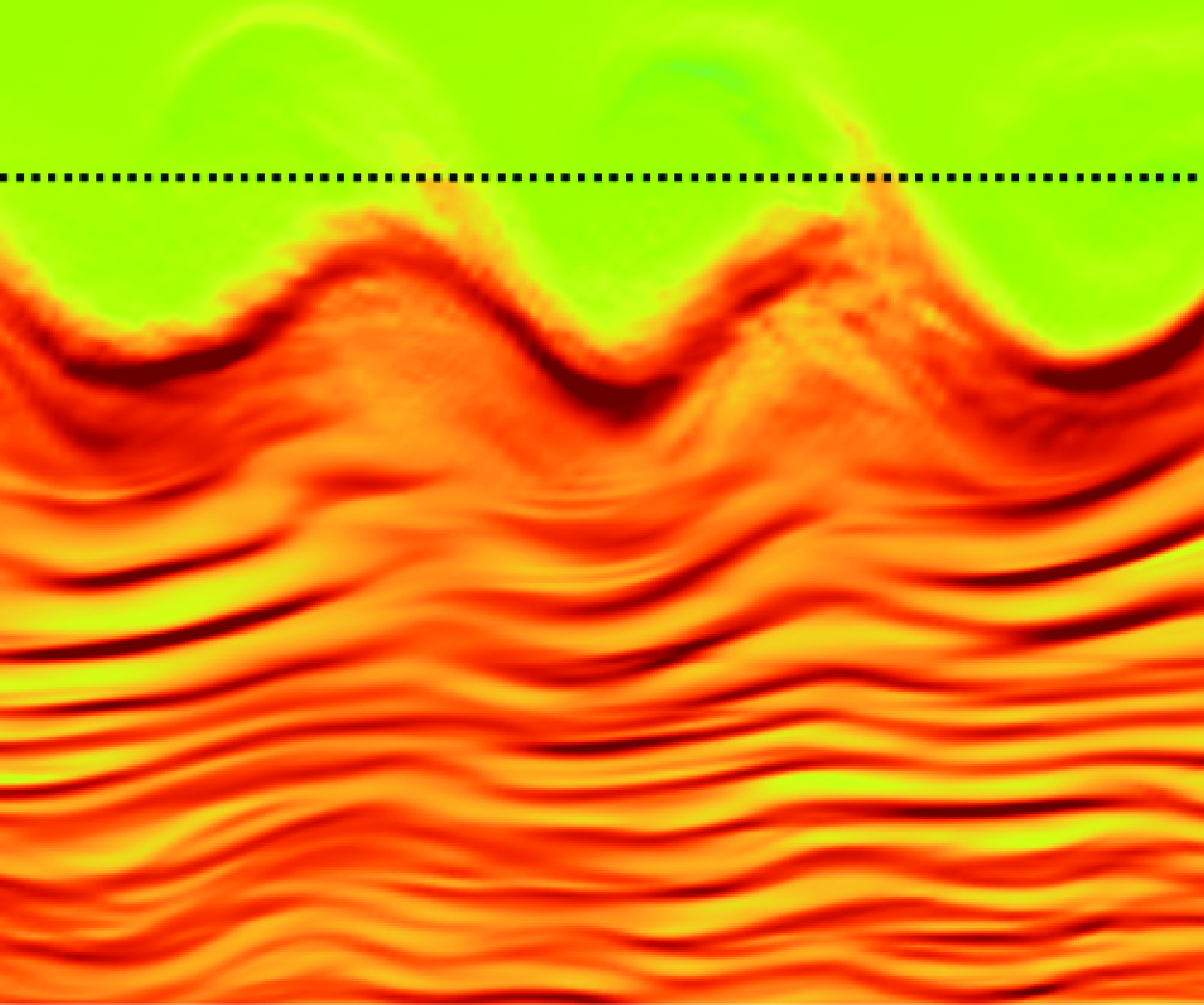
Figure 3. Side views of the cross-stream averaged temperature gradients $\partial \langle \theta \rangle _{y}/\partial z$ . Snapshots at around $tf=1$ are shown for four representative cases: $(a)$ NC, no canopy, with the Stokes drift; $(b)$ NC-NSW, no canopy, no Stokes drift; $(c)$ C0.3, canopy density of 0.3 m $^{-1}$ ; $(d)$ C3, canopy density of 3 m $^{-1}$ ; $(e)$ C3-WG, canopy density of 3 m $^{-1}$ and a weaker geostrophic current; and $(f)$ C3-NG, canopy density of 3 m $^{-1}$ and no geostrophic current. Black dotted lines represent the canopy base depth (lines also included in the no-canopy cases for comparison purposes). Note that the sponge layer is not shown in the plots.

Along with variations in the OML depth, distinct flow patterns are observed across different simulations. In the side-view snapshots of the two cases without the canopy (figures 3 a and 3 b), more pronounced internal wave patterns are observed in the case with Stokes drift (NC) compared with the case without Stokes drift (NC-NSW). This comparison indicates the importance of Langmuir turbulence, arising from the interaction between surface waves and wind-driven currents, for internal wave generation (Polton et al. Reference Polton, Smith, MacKinnon and Tejada-Martínez2008) (details examined later).

In the presence of a canopy, patterns resembling KH instability (e.g. Kundu et al. Reference Kundu, Cohen and Dowling2015) emerge near the canopy bottom edge. The dominant wavelength of these patterns positively depends on the canopy density (comparing figures 3 c and 3 d). Additionally, the KH-type patterns also lead to the radiation of internal waves in the deeper water. In the case with a weaker $u_g$ , the dominant wavelength of the KH structures decreases (figure 3 e). In the absence of a geostrophic current ( $u_g = 0$ ), the KH structures do not occur (figure 3 f), and the internal wave patterns resemble those observed without a canopy.

The impact of Stokes drift on the canopy shear layer is minimal. The two canopy cases, with and without Stokes drift (C3 and C3-NSW, figure 2 a), exhibit similar changes in OML depth, and the KH structures in these two cases are also consistent (case C3-NSW not shown). This result aligns with expectations, given that the KH instability primarily relates to the vertical shear generated by the canopy, and Stokes drift is weak at that depth. In this study, we focus on the canopy simulation with Stokes drift (case C3) to facilitate comparison with the Langmuir turbulence simulation (case NC).

Overall, the presence of a canopy significantly impacts OML dynamics, including the emergence of KH-type patterns, the deepening of the OML, and the radiation of internal waves in the underlying stratification. Further analysis of these effects will be conducted in the following sections. It is also worth mentioning that velocity and temperature profiles, as well as the KH-type patterns, evolve over time as the OML depth gradually increases. The temporal evolution of velocity and temperature dynamics will be discussed in § 3.3.

Figure 4. Velocity and temperature profiles in four representative simulations at the final simulation time $tf=9$ . $(a,b)$ Horizontally averaged streamwise velocity $\langle \overline {u}\rangle _{xy}$ and cross-stream velocity $\langle \overline {v}\rangle _{xy}$ , both normalized by the geostrophic velocity $u_g=0.2\,\rm m\,s^-{^1}$ . $(c,d)$ Horizontally averaged temperature $\langle \overline {\theta }\rangle _{xy}$ and the vertical gradient of temperature. Horizontal dotted lines represent the canopy base depth.

3.2. Final velocity and temperature profiles

Figure 4 compares the velocity and temperature profiles for four representative cases (the same as the ones depicted in figure 3), namely NC, NC-NSW, C0.3 and C3, at the final simulation time $tf=9$ , when the OML depth reaches its maximum. In the two cases without a canopy, the horizontal velocity components $u$ and $v$ exhibit a more uniform distribution with depth in the presence of Stokes drift and Langmuir turbulence compared with their absence (cases NC and NC-NSW, represented by the two black lines in figures 4 a and 4 b). This aligns with the findings by McWilliams et al. (Reference McWilliams, Sullivan and Moeng1997), indicating that Langmuir turbulence leads to more efficient vertical momentum transport than wind-driven shear turbulence.

A peak in the vertical temperature gradient $\partial \langle \theta \rangle _{xy}/\partial z$ forms as the OML deepens (figure 4 $d$ ), consistent with results from previous studies (e.g. Li & Garrett Reference Li and Garrett1997). This local maximum of the vertical temperature gradient is commonly referred to as a pycnocline (here a thermocline), located between the OML and the underlying uniform stratification (e.g. Taylor & Sarkar Reference Taylor and Sarkar2007). The case with the Stokes drift demonstrates a deeper thermocline and a more notable peak in $\partial \langle \theta \rangle _{xy}/\partial z$ , because Langmuir turbulence can enhance vertical mixing within the OML (Li & Garrett Reference Li and Garrett1997; Kukulka et al. Reference Kukulka, Plueddemann, Trowbridge and Sullivan2010). Nevertheless, the initial OML depth $h_0$ is greater than the threshold value of 10–17 $u_*/N$ , where Langmuir turbulence is expected to cause rapid OML deepening (Li & Garrett Reference Li and Garrett1997). As a result, the observed increase in the OML depth is relatively small, e.g. around 10%, in the absence of a canopy.

When a canopy is present in the OML, the streamwise velocity is significantly decelerated near the sea surface due to the canopy drag force, leading to the formation of a shear layer below the canopy (figure 4 $a$ ). The extent of deceleration and the thickness of the shear layer exhibit a positive dependence on the canopy density (comparing cases C1 and C3). Additionally, a positive cross-stream velocity arises (to the left of the streamwise current) due to the combined effects of the Ekman spiral and canopy drag (Yan et al. Reference Yan, McWilliams and Chamecki2021) (figure 4 $b$ ).

The shear layer attached to the canopy results in the emergence of KH-type patterns and significant deepening of the OML. By the end of the simulation, the local maximum of the vertical temperature gradient $\partial \langle \theta \rangle _{xy}/\partial z$ reaches close to three times its initial value in the case with the highest canopy density (figure 4 $d$ ). The increased OML depth generally corresponds with the thickness of the canopy shear layer (comparing figures 4 $a$ and 4 $d$ ), suggesting that canopy-generated shear is the predominant mechanism driving mixing and OML deepening. In addition, a secondary peak of $\partial \langle \theta \rangle _{xy}/\partial z$ emerges within the canopy in case C3 (e.g. at around $z/h_b=-0.3$ in figure 4 $d$ ; also see figure 3 $d$ ). The formation of this secondary peak is attributed to the upward advection of gradients from the thermocline by the KH-type structures, as well as the localized inhibition of turbulence and mixing inside the canopy.

3.3. Kelvin–Helmholtz instability

Patterns resembling KH instability emerge as the canopy shear layer interacts with the underlying stratification (figure 3). In this section, we further investigate characteristics of the observed KH-type patterns. The KH instability occurs when the destabilizing effect of velocity shear overcomes the stabilizing effect of stratification (e.g. Kundu et al. Reference Kundu, Cohen and Dowling2015). The gradient Richardson number $Ri_g$ compares the two competing effects and is defined as

(3.4) \begin{equation} Ri_g = \frac {N^2}{S^2}, \end{equation}

where $N$ is the buoyancy frequency as described by (2.7) and $S$ is the vertical shear given by

(3.5) \begin{equation} S = \sqrt {\left (\frac {\partial {u}}{\partial {z}}\right )^2+\left (\frac {\partial {v}}{\partial {z}}\right )^2}. \end{equation}

The $Ri_g$ is calculated from the horizontally averaged velocity and temperature profiles, and $Ri_g\lt 0.25$ is found in the canopy shear layer when the KH-type structures occur (please refer to the Supplementary material for the movie of $Ri_g$ ). This is consistent with the condition favourable for the growth of KH instability and mixing obtained from linear stability analysis (Miles Reference Miles1961; Howard Reference Howard1961).

Figure 5. $(a)$ The dominant $x$ -direction wavenumber $k_{x,peak}$ versus canopy shear layer thickness $\delta _s$ . Different colours represent simulations with different canopy density and $u_g$ (C0.1–C3 and C3-WG, see the legend), and each point corresponds to a time interval of every $tf=0.0015$ . $(b)$ The dominant phase speed $c_{x,peak}$ of the KH-type structures versus the current speed of the inflection point in the shear layer. Note that the results are normalized by $u_g=0.1\,\rm m\,s^-{^1}$ in case C3-WG and by $u_g=0.2\,\rm m\,s^-{^1}$ in all the other cases.

Moreover, the wavelength of the most unstable mode of KH instability is typically 7–8 times the shear layer thickness (Sutherland Reference Sutherland and Rahman2005). The canopy shear layer thickness $\delta _s$ is calculated as (e.g. Finnigan Reference Finnigan2000)

(3.6) \begin{equation} \delta _s = \frac {max (\langle u\rangle _{xy})-min (\langle u\rangle _{xy})}{max (\left |\frac {\partial {\langle u\rangle _{xy}}}{\partial {z}}\right |)}, \end{equation}

i.e. the maximum velocity difference in the horizontally averaged profile divided by the maximum shear. The dominant wavenumber $k_{x,peak}$ is estimated from the peak in the $x$ -direction wavenumber spectrum. Here we investigate the KH wavelength scaling (Sutherland Reference Sutherland and Rahman2005) by examining the following relationship:

(3.7) \begin{equation} k_{x,peak}\delta _s \approx 1. \end{equation}

The scaling in (3.7) generally applies across all simulations spanning a range of canopy densities (figure 5 $a$ ). Increased canopy density typically results in increased shear layer thickness and consequently longer wavelengths in the induced KH-type patterns (cases C0.1 to C3). This dependence on canopy density is also apparent when comparing the side views in figures 3 $(c)$ and 3 $(d)$ . Additionally, a weaker geostrophic current results in a thinner shear layer, leading to shorter KH wavelengths (cases C3 and C3-WG, figure 5 $a$ ; also see figures 3 $d$ and 3 $e$ ). Moreover, each simulation with a specific canopy density exhibits variations in KH wavelength (figure 5 $a$ ), which relates to the temporal evolution of the canopy shear layer and KH-type patterns, as further discussed in the following paragraph.

While a representative snapshot has been shown in a previous section in figure 3, the KH-type patterns also evolve over time. Here we take case C3 as an example to illustrate the evolving features in the canopy shear layer (figure 6). The simulations are initiated with a uniform velocity profile of $u=u_g$ . As the canopy drag decelerates the ocean current, a shear layer rapidly develops beneath the canopy (e.g. for $tf\lt 0.5$ ) and the shear layer thickness remains relatively stable after $tf=0.5$ . Note that the growth of the shear layer thickness occurs within a relatively short time (figure 6 $a$ ) compared with the deepening of the OML (figure 6 $b$ ). At an earlier stage when the shear layer thickness is smaller (e.g. $tf=0.25$ in figure 6 $a$ ), the dominant KH wavelength is correspondingly shorter (comparing figure 6 $c$ with figure 3 $d$ ), as predicted by the scaling relationship in (3.7). As time progresses, the KH wavelength increases with the thickening of the shear layer (see the movie in the Supplementary material). Eventually, the shear layer becomes mismatched with the stratification due to the continuous deepening of the thermocline, resulting in a regime that deviates from classical KH instability.

Figure 6. Time evolution of the velocity and temperature field in case C3. $(a)$ Vertical profiles of horizontally averaged streamwise velocity $\langle \overline {u}\rangle _{xy}$ , at $tf=0.3$ , 0.5 and 9. $(b)$ Vertical profiles of horizontally averaged temperature $\langle \overline {\theta }\rangle _{xy}$ , at every $tf=1$ . $(c,d)$ Side views of the cross-stream averaged temperature gradients $\partial \langle \theta \rangle _{y}/\partial z$ at $tf=0.3$ and $tf=3$ , representing stages earlier and later than figure 3 $(d)$ , respectively.

It is worth noting that the canopy-generated structures may comprise of a combination of KH waves and Holmboe waves (Carpenter et al. Reference Carpenter, Balmforth and Lawrence2010; Zagvozkin et al. Reference Zagvozkin, Vorobev and Lyubimova2019), since their distinction is often less clear in an asymmetric stratified profile (such as the one used in this study). The KH instability usually occurs in the presence of relatively strong velocity shear that satisfies $Ri_g\lt 0.25$ , whereas Holmboe instability can arise from the interaction between shear and stratification even when $Ri_g\gt 0.25$ . The KH waves typically travel at a phase speed close to the current speed of the inflection point ( $u_{infl}$ , here defined as the point where $|\partial u/\partial z|$ reaches its maximum). However, the propagating phase speed of Holmboe waves can be significantly different from $u_{infl}$ (e.g. Alexakis Reference Alexakis2007; Carpenter et al. Reference Carpenter, Balmforth and Lawrence2010).

The relationship between $u_{\textit{infl}}$ and the dominant phase speed $c_{p,peak}=\omega _{peak}/k_{x,peak}$ is examined in figure 5 $(b)$ . Although $c_{p,peak}$ is in general close to $u_{infl}$ across all simulations, deviations are evident, particularly for the highest canopy density (case C3), implying the presence of Holmboe waves. As time progresses, while the shear layer remains attached to the canopy bottom, the thermocline continues to deepen as the OML depth increases. Consequently, at later stages, the thermocline no longer coincides with the shear layer, which may lead to patterns resembling Holmboe waves (figure 6 $d$ ). The magnitude of these canopy-generated structures eventually diminishes as the mixed layer continues deepening and the thermocline becomes displaced from the shear layer.

Distinguishing between KH modes and Holmboe modes is challenging in our non-idealized scenario, and the cases presented here likely exhibit characteristics of both. We therefore refer to all these canopy-induced patterns as KH-type. In the following analyses, we primarily focus on a representative time around $tf=1$ when the KH-type structures and internal waves are most prominent (the same time as shown in figure 3). Cases without a canopy will also be analysed at the same representative time to serve as comparisons.

Figure 7. $(a)$ The TKE profiles in four representative cases, normalized by the square of the friction velocity $u_*$ . $(b)$ The vertical component of TKE. $(c)$ Ratio of the vertical component to the total TKE. $(d)$ Skewness of the vertical turbulent velocity. The results correspond to around $tf=1$ , same as the time when the side views in figure 3 are shown. Note that the ratio and skewness are not shown for regions where TKE $/u_*^2\lt 1$ . Horizontal dotted lines represent the canopy base depth.

3.4. Turbulence

We first calculate the turbulence kinetic energy (TKE) for four representative cases (NC, NC-NSW, C0.3 and C3), where

(3.8) \begin{equation} \textrm {TKE} = \frac {1}{2}\left ( \overline {u'^2}+\overline {v'^2}+\overline {w'^2} \right ). \end{equation}

The cases with a canopy display a noticeable increase in TKE at the bottom edge of the canopy (figure 7 $a$ ), corresponding to the canopy shear layer turbulence. Note that while the calculated TKE accounts for high-frequency turbulent motions induced by shear and KH instability, it does not include the energy directly associated with the KH-type structures, as these are classified as lower-frequency motions according to the definition in (3.1). The lower-frequency motions will be examined in the following section.

Langmuir turbulence (case NC, no canopy, with the Stokes drift) is characterized by a relatively higher energy content in the vertical component (figure 7 $c$ ), and similar turbulence anisotropy has been reported by McWilliams et al. (Reference McWilliams, Sullivan and Moeng1997). In comparison, canopy shear layer turbulence typically exhibits less turbulence anisotropy (cases C0.3 and C3, e.g. at around $z/h_0=-0.8$ to $-1.5$ ).

The skewness of the vertical turbulence component, defined as $\overline {{w'}^3}/\overline {{w'}^2}^{3/2}$ , is examined to illustrate the various turbulence characteristics (figure 7 $d$ ). Langmuir turbulence (case NC) is featured by its distinctively negative skewness of vertical velocity (McWilliams et al. Reference McWilliams, Sullivan and Moeng1997). This negative skewness is attributed to stronger downward motions confined within narrower regions of Langmuir circulations, compared with broader and weaker upward motions. For shear layer turbulence generated at the canopy bottom (cases C0.3 and C3), the vertical velocity skewness is positive, e.g. in the lower-half of the canopy. This positive skewness indicates the dominance of sweep events that brings high-momentum fluid into the canopy, consistent with those found in classical canopy flows (Raupach & Thom Reference Raupach and Thom1981; Katul et al. Reference Katul, Kuhn, Schieldge and Hsieh1997; Poggi et al. Reference Poggi, Porporato, Ridolfi, Albertson and Katul2004). It is also worth noting that the skewness sign in the suspended canopy is opposite to that of submerged benthic canopies; here, the sweep events are characterized by intensified positive vertical velocities into the canopy. Additionally, in the upper-half of the canopy where the influence of Stokes drift is greater, negative skewness is observed, which represents a characteristic of canopy-modulated Langmuir turbulence (Bo et al. Reference Bo, McWilliams, Yan and Chamecki2024b ).

Figure 8. Terms in the TKE budget (3.9) for case NC (no canopy, with the Stokes drift) and case NC-NSW (no canopy, no Stokes drift) at around $tf=1$ : $(a)$ shear production associated with the streamwise velocity; $(b)$ Stokes production; $(c)$ dissipation; $(d)$ buoyancy production; $(e)$ pressure work (vertical divergence of pressure flux); $(e)$ pressure flux. Only the dominant terms are shown. Note the differences in the horizontal axis range.

Further analysis of the TKE budget is conducted to understand the mechanisms of turbulence generation,

(3.9) \begin{eqnarray} \frac {\text {D}}{\text {D}t} \textrm {TKE} = - \overline {u_i' u_j'}\frac {\partial {\overline {u_i}}}{\partial {x_j}} - \overline {u'w'}\frac {\partial {u_s}}{\partial {z}} - \epsilon - \overline {u'_{i} F'_{D,i}} + \alpha g\overline {w'\theta '} - \frac {1}{\rho }\frac {\partial {}}{\partial {x_j}}\overline {u'_j p'} \nonumber \\ - \frac {1}{2}\frac {\partial {}}{\partial {x_j}}\overline {u'_iu'_iu'_j} + \frac {\partial {}}{\partial {x_j}}\overline {u'_i\tau '_{ij}}, \\\nonumber\end{eqnarray}

where the material derivative is defined as $\text {D}/\text {D}t = \partial /\partial t + \overline {u_j}\partial /\partial x_j + u_s\partial /\partial x$ . Note that we have used Einstein notation. The first and second terms on the right-hand side represent shear production and Stokes production, respectively. The third term $\epsilon$ denotes SGS dissipation, and the fourth term stands for canopy drag dissipation. The fifth term represents buoyancy production, followed by the sixth term that denotes pressure work. The last two terms represent TKE transport associated with the resolved stress and SGS stress.

In the two cases without a canopy (figures 8 $a$ and 8 $b$ ), shear production is the primary source of wind-driven shear turbulence (case NC-NSW), while Stokes production predominates for Langmuir turbulence (case NC). The shear production and Stokes production terms are generally balanced by the dissipation term (figure 8 $c$ ), with minimal influences from other source or sink terms or TKE transport.

Figure 9. Terms in the TKE budget (3.9) for case C3 (with the highest canopy density): red lines, at $tf=1$ ; blue lines, at $tf=0.3$ ; black lines, at $tf=9$ ; $(a,b)$ shear production associated with the streamwise velocity and cross-stream velocity, respectively; $(c)$ Stokes production; $(d)$ dissipation; $(e)$ canopy drag dissipation; $(f)$ TKE transport; $(g)$ buoyancy production; $(h)$ pressure work (vertical divergence of pressure flux); $(i)$ pressure flux. Note the differences in the horizontal axis range. Horizontal dotted lines represent the canopy base depth.

Negative buoyancy production is evident near the thermocline (figure 8 $d$ ), which indicates the energy transfer from TKE to potential energy, contributing to mixing and OML deepening. Langmuir turbulence induces stronger buoyancy fluxes than wind-driven shear turbulence, consistent with the greater increase in OML depth in case NC compared with case NC-NSW (figure 2 $a$ ). Moreover, negative pressure fluxes occur below the thermocline in the simulation with Langmuir turbulence (figure 8 $f$ ), corresponding to the observed downward-propagating internal waves (figure 3 $a$ ). The vertical divergence of pressure fluxes (the pressure work term) (figure 8 $e$ ) is in general much smaller than the Stokes production and dissipation terms, suggesting that internal wave radiation has a small influence on TKE. Nevertheless, pressure work has a comparable magnitude to buoyancy production, and this underscores the potential importance of internal waves for mixed layer deepening (Taylor & Sarkar Reference Taylor and Sarkar2007).

In the presence of a canopy (case C3, $tf=1$ , red lines in figure 9), a notable peak in shear production occurs near the canopy bottom edge where KH-type patterns emerge. Stokes production has a small magnitude compared with shear production, and this explains why removing the Stokes drift leads to minimal changes to the OML depth when a canopy is present (comparing cases C3 and C3-NSW). The TKE transport term indicates a loss of TKE in the canopy shear layer where production peaks and a gain within the canopy (figure 9 $e$ ), consistent with findings from classical canopy flow studies (e.g. Finnigan Reference Finnigan2000). In addition, a negative peak in pressure work is observed at the canopy base, corresponding to the canopy-induced KH-type patterns and radiated internal waves.

Negative buoyancy production is evident in the canopy shear layer, contributing to mixing at the thermocline (figure 9 $g$ ). The buoyancy production term is small compared with the shear production term. This buoyancy mixing associated with the canopy and KH-type patterns is consistent with the principles of the classical Osborn–Cox model (Osborn & Cox Reference Osborn and Cox1972), wherein sharp gradients of oceanic microstructures usually play a pivotal role in vertical mixing. It is also worth noting that buoyancy production here can be around an order of magnitude larger than that without a canopy (case NC), thus leading to more pronounced OML deepening in the presence of a canopy (figure 2 $a$ ).

While the above analysis focuses on $tf=1$ , the TKE budget at earlier ( $tf=0.3$ ) and later ( $tf=9$ ) stages is also presented in figure 9 (blue and black lines). In general, the vertical distribution of the shear production, dissipation and TKE transport terms is similar across different times. However, the magnitudes of shear production and dissipation are greater at later times, as turbulence develops with time. Additionally, at the later stage, the peaks of buoyancy production and pressure flux occur at greater depths (black lines in figures 9 $g$ and 9 $i$ ), because the thermocline deepens. Moreover, negative buoyancy production is not observed at the earlier stage (red line in figure 9 $g$ ). Instead, positive values of buoyancy production occur, likely indicating convectively unstable regimes, as dense filaments are advected upward in the initial stages of KH instability.

3.5. Internal waves beneath the OML

Alongside the deepening of the OML, internal waves can be generated in the underlying stratification as flow processes in the OML interact with the thermocline. As outlined in a previous section, Langmuir turbulence (case NC, no canopy) and the canopy-induced KH-type structures (cases C0.1–C3) can both lead to internal wave radiation beneath the OML (figure 3). In this section, we further analyse the properties of internal waves. Here internal wave computations are based on vertical velocity gradients $\partial w/\partial z$ following Taylor & Sarkar (Reference Taylor and Sarkar2007), as $\partial w/\partial z$ reveals internal wave patterns more clearly. The spectra of the vertical velocity $w$ generally provide consistent information with those of $\partial w/\partial z$ .

Figure 10. Side-view and cross-sectional plots of vertical velocity gradients at around $tf=1$ in case NC. $(a)$ The cross-stream averaged vertical velocity gradient $\partial \langle w\rangle _{y}/\partial z$ in the $x-z$ plane. $(b)$ The vertical velocity gradient $\partial w/\partial z$ at $y=0$ in the $x-z$ plane. $(c)$ The $x$ -direction averaged vertical velocity gradient $\partial \langle w\rangle _{x}/\partial z$ in the $y-z$ plane. $(d)$ The vertical velocity gradient $\partial w/\partial z$ at $x=0$ in the $y-z$ plane.

Figure 11. Spectra of vertical velocity gradients $\partial w/\partial z$ in case NC, versus $x$ - or $y$ -wavenumber or frequency. $(a{-}c)$ Spectra of the $x$ - or $y$ -direction averaged results. $(e,f)$ The $x$ - or $y$ -direction average of the spectra at every $x$ - or $y$ -location. Dashed lines represent the average between $z/h_0=-1$ to $0$ (within the OML), and solid lines represent the average between $z/h_0=-3$ and $-2$ (below the thermocline). Vertical red lines indicate the buoyancy frequency $N$ . Note that the frequency in the spectral plot is generally much higher than $N$ due to the Doppler shift caused by the geostrophic current. In the text, intrinsic internal wave frequencies are analysed after removing the Doppler shift effect.

In case NC, the side-view plots (figures 10 $a$ and 10 $b$ ) indicate propagating internal waves in the $x-z$ plane. Internal wave patterns are more discernible when averaging in the $y$ -direction, whereas examining a slice at any specific $y$ -location tends to obscure these patterns. It is worth noting that internal waves also propagate in the $y$ -direction, as illustrated in the cross-sectional plots (figures 10 $c$ and 10 $d$ ). Plotting $\partial u/\partial z$ instead of $\partial w/\partial z$ will enhance the clarity of internal wave patterns in the $x-z$ plane, with less discrepancy between the $y$ -direction average and a specific $y$ -location. However, $\partial u/\partial z$ does not reveal any wave patterns in the $y$ -direction, and we therefore use $\partial w/\partial z$ in our analysis.

The dispersion relation for non-rotating linear internal waves is given by

(3.10) \begin{equation} \omega _i = N\cos \Theta , \end{equation}

where $\omega _{i}$ is the intrinsic frequency, $N$ is the buoyancy frequency as defined in (2.7) and $\Theta$ is the angle between the wavenumber vector and the horizontal axis. While near-inertial oscillations can also propagate downwards below the OML (Bell Reference Bell1978), the observed wave frequency is close to $N$ and significantly higher than the Coriolis frequency $f$ , and we have thus neglected the influence of planetary rotation.

In the $x$ -direction wavenumber spectrum of case NC (figure 11 $a$ ), a peak at $k_xh_0=3.6$ is evident below the thermocline, representing the dominant wavenumber of the downward propagating internal waves, and this contrasts with the broadband turbulence observed in the surface boundary layer. Correspondingly, a peak frequency of around $\omega _{peak}/f=300$ is observed in the time spectrum (figure 11 $c$ ). The intrinsic internal wave frequency $\omega _{i}$ is estimated by accounting for the Doppler shift:

(3.11) \begin{equation} \omega _i = \omega _{peak} - k_{x,peak} u_g. \end{equation}

Here the intrinsic frequency is $\omega _{i}/f\approx 20$ , which is smaller than the buoyancy frequency $N/f=44$ , suggesting a wave propagation angle $\Theta$ of around $60^\circ$ . This in general agrees with the angle estimated from

(3.12) \begin{equation} \Theta = \cos ^{-1}\left (\sqrt {\frac {k_{x,peak}^2+k_{y,peak}^2}{k_{x,peak}^2+k_{y,peak}^2+k_{z,peak}^2}}\right ), \end{equation}

so the dispersion relation of freely propagating internal waves is satisfied. Nevertheless, the non-monotonic nature of the radiated internal waves may lead to uncertainty when applying the dispersion relation in (3.10). Additionally, we note that while the wavenumber and frequency peaks of internal waves are evident in the $x$ - or $y$ -direction averaged field, they are less clear when we calculate spectra based on slices at any specific $x$ - or $y$ -location (figure 11 $d{-}f$ ).

The presence of a narrow range of dominant wavenumbers and frequencies in internal waves is consistent with the selection mechanism proposed by Gibson et al. (Reference Gibson, Bondur, Norris Keeler and Leung2006) and Taylor & Sarkar (Reference Taylor and Sarkar2007). While energy is distributed across a wide range of frequencies in boundary layer turbulence, internal waves with either low or high frequencies exhibit slow vertical propagation speeds or rapid viscous decay rates. Consequently, an intermediate dominant frequency emerges as waves propagate beneath the OML, although they are excited by broadband turbulence.

The analysis above has focused on internal waves associated with Langmuir turbulence (case NC, no canopy, with the Stokes drift). Wind-driven shear turbulence (case NC-NSW, no canopy, no Stokes drift) is expected to generate internal waves through a similar mechanism. However, internal wave energy is much weaker in case NC-NSW compared with case NC, with less discernible wave patterns (comparing figures 3 $a$ and 3 $b$ ) and a less distinctive peak in the wavenumber spectrum (not shown). We attribute this difference to the fact that Langmuir turbulence, compared with wind-driven shear turbulence, results in stronger mixing in the OML (McWilliams et al. Reference McWilliams, Sullivan and Moeng1997; Li & Garrett Reference Li and Garrett1997) and more deeply penetrating vertical velocities that interact with the stratification (Polton & Belcher Reference Polton and Belcher2007), which thus leads to more pronounced internal waves (Chini & Leibovich Reference Chini and Leibovich2003; Polton et al. Reference Polton, Smith, MacKinnon and Tejada-Martínez2008).

Figure 12. Side views of vertical velocity gradients at around $tf=1$ in case C3. $(a)$ The cross-stream average vertical velocity gradient $\partial \langle w\rangle _{y}/\partial z$ . $(b)$ The vertical velocity gradient $\partial w/\partial z$ at $y=0$ .

In the presence of a canopy, internal wave patterns below the thermocline are primarily associated with the KH-type structures in the canopy shear layer (figure 12). A distinct peak at $k_x h_0=1.5$ is noticeable in the $x$ -direction wavenumber spectrum, both within the surface boundary layer and below the thermocline (figures 13 $a$ and 13 $d$ ). This corresponds to an observed peak frequency of around $\omega _{peak}/f=50$ (figures 13 $c$ and 13 $f$ ). In contrast to the Langmuir turbulence simulation where internal waves propagate in both the $x$ - and $y$ -directions, the simulation with a canopy exhibits minimal variations in the $y$ -direction, with no apparent discrepancy between the cross-stream averaged results and any specific $y$ -location (e.g. comparing figures 12 $a$ and 12 $b$ ). Multiple peaks in the $y$ -direction wavenumber spectrum are observed (figure 13 $e$ ), which likely represent cross-stream structures associated with secondary instability in KH and Holmboe waves (e.g. Smyth & Peltier Reference Smyth and Peltier1991; Mashayek & Peltier Reference Mashayek and Peltier2013; Mashayek et al. Reference Mashayek, Caulfield and Peltier2013; VanDine et al. Reference VanDine, Pham and Sarkar2021). Our model is unable to fully resolve these secondary structures. However, it is important to note that the energy associated with cross-stream structures is generally much lower than that of the streamwise structures. We therefore primarily focus on the streamwise structures that are more dominant in OML mixing. In the simulation with doubled horizontal resolution, consistent peaks are observed in the $y$ -direction wavenumber spectrum.

Figure 13. Spectra of vertical velocity gradients $\partial w/\partial z$ in case C3, versus $x$ - or $y$ -wavenumber or frequency (a similar set of panels to figure 11). $(a{-}c)$ Spectra of the $x$ - or $y$ -direction averaged results. $(e,f)$ The $x$ - or $y$ -direction average of the spectra at every $x$ - or $y$ -location. Dashed lines represent the average between $z/h_0=-1$ to $0$ (within the OML), and solid lines represent the average between $z/h_0=-3$ and $-2$ (below the thermocline).

The dominant intrinsic frequency of internal waves is estimated to be $\omega _{i}/f\approx -50$ by considering the Doppler shift in (3.11). The negative value indicates that internal waves would propagate in the $-x$ -direction when observed in a coordinate frame moving with the geostrophic current $u_g$ . This is consistent with analysis in the previous section (figure 5 $b$ ), where the phase speed of KH-type structures is close to the current speed at the inflection point ( $u_{infl}\lt u_g$ ). The magnitude of the intrinsic frequency $\omega _i$ is close to the buoyancy frequency $N$ , suggesting horizontal wave propagation according to the dispersion relation (3.10). This aligns with observations from the side-view plots (figure 12), where the wave phase lines are nearly vertical. In addition to the dominant internal wave patterns that primarily propagate horizontally (with a peak wavenumber and frequency associated with the KH-type structures), internal waves with other frequencies are also excited in the canopy simulation (figure 12). These waves propagate in the vertical direction, as indicated by their inclined phase lines.

Note that a sponge layer is applied at the bottom boundary to avoid internal wave reflection. We also conduct a simulation with doubled domain depth to examine any potential reflection (case C3-DEEP, details provided in appendix A). The case with the highest canopy density is chosen because it results in the deepest OML and KH-type structures closest to the bottom boundary, making it most susceptible to the influence of internal wave reflection. Overall, the wave spectra show negligible differences between cases C3 and C3-DEEP, indicating that the sponge layer effectively prevents wave reflection (appendix A).

3.6. The OML deepening and nutrient entertainment

The presence of a canopy can significantly deepen the OML, and both canopy-induced turbulence and lower frequency motions associated with KH-type structures have the potential to enhance mixing. Moreover, since nutrient transport in the ocean is typically influenced by OML dynamics, the presence of a canopy may thus substantially impact the vertical distribution of nutrients. In this section, we quantify the vertical transport processes associated with the canopy. The velocity has been decomposed into turbulence ( $\textbf {u}'$ ) and low-frequency motions ( $\overline {\textbf {u}}$ , averaged every 75 s) based on (3.1). We further decompose the low-frequency velocity as

(3.13) \begin{equation} \overline {\textbf {u}} = \widetilde {\overline {\textbf {u}}} + \overline {\textbf {u}}^l, \end{equation}

where the tilde denotes the overall time average, and the superscript $l$ denotes low-frequency fluctuations around the time average. The complete flow decomposition is thus given by

(3.14) \begin{equation} \textbf {u} = \widetilde {\overline {\textbf {u}}} + \overline {\textbf {u}}^l + \textbf {u}'. \end{equation}

The term $\textbf {u}'$ denotes fluctuations associated with turbulence, while other lower-frequency fluctuations, such as the KH-type structures and internal waves, are represented by $\overline {\textbf {u}}^l$ . Likewise, any scalar $\phi$ , e.g. temperature and nutrient concentration, can be decomposed into

(3.15) \begin{equation} \phi = \widetilde {\overline {\phi }} + \overline {\phi }^l + \phi '. \end{equation}

The total time-averaged vertical flux is thus written as

(3.16) \begin{equation} \widetilde {\overline {w\phi }} = \widetilde {\overline {w}^l\overline {\phi }^l} + \widetilde {\overline {w'\phi '}}. \end{equation}

Note that there is no vertical flux driven by the mean flow because $\widetilde {\overline {w}}=0$ .

Figure 14. Vertical fluxes of momentum and temperature for case NC (black) and case C3 (red), time-averaged from $tf=0$ to $tf=9$ and horizontally averaged. $(a,b)$ Turbulent fluxes of momentum and temperature. $(c,d)$ Fluxes driven by lower-frequency motions. Fluxes are normalized by $u_*$ and $\Delta \theta =1\,\rm K$ .

The momentum and temperature fluxes of cases NC and C3 are compared in figure 14. The intensified turbulence within the canopy shear layer considerably enhances vertical temperature mixing compared with the case without a canopy. Moreover, lower-frequency motions also substantially contribute to temperature mixing, with a comparable magnitude to the contribution from turbulence. This underscores the dual role of the canopy, which generates turbulence and enhances turbulent mixing, while also directly leading to mixing through the lower-frequency KH-type structures. The momentum flux is primarily dominated by turbulence in the canopy shear layer, with lower-frequency velocities exhibiting weaker correlation than turbulence. As a contrast, in the absence of a canopy (case NC), although internal waves are generated, these lower-frequency motions have a negligible influence on temperature and momentum mixing. This indicates that the deepening of the OML is primarily driven by Langmuir turbulence rather than the radiated internal waves.

Figure 15. $(a)$ Nutrient profiles for case NC (black) and case C3 (red), at $tf=9$ . The thin grey line shows the initial nutrient profile at $tf=0$ . $(b,c)$ Vertical nutrient fluxes driven by turbulence and lower-frequency motions, respectively. These fluxes are time-averaged from $tf=0$ to $tf=9$ and horizontally averaged. Fluxes are normalized by $u_*$ and $\Delta C_N=10000$ $\unicode{x03BC}\rm mol\,m^-{^3}$ .

Furthermore, the presence of a canopy also significantly enhances vertical nutrient transport (figure 15). Similar to temperature fluxes, both turbulence and lower-frequency KH structures are important factors in enhancing nutrient entrainment into the OML. The nutrient concentration near the sea surface is increased by more than twofold compared with the case without a canopy. Considering that the present study on the canopy flow is motivated by macroalgal farming, the increased nutrient concentration fosters a favourable condition for macroalgal growth. This provides a self-sustaining solution for nutrient supply and farm maintenance through continuous passive entrainment. Note that a secondary peak in nutrient flux occurs near the sea surface in the case with the canopy (at $z/h_0=-0.3$ in figure 15 $b$ ). A similar secondary peak is found in the temperature flux (figure 14 $b$ ). This is because the KH structures advect strong gradients from the thermocline to near the sea surface (see figure 3 $d$ ), resulting in locally increased fluxes as these gradients are mixed by turbulence within the canopy.