2.1. Problem definition

Consider a heated vertical surface immersed in a stratified medium such that the temperature difference between the surface and the ambient medium remains constant along the entire length of the vertical surface. The temperature difference between the vertical surface and the ambient surroundings causes the fluid to rise upwards and form a NCBL on the surface. However, due to the stable ambient stratification, the NCBL does not grow with increasing height but attains a constant boundary layer thickness and has temporally and spatially invariant velocity and buoyancy profiles. The flow schematic is shown in figure 2. From the figure, it is clear that the buoyancy layer features zones of flow reversal and temperature deficit in the outer layer, making it drastically different from unstratified vertical NCBLs where no such flow reversal or temperature deficit is observed (cf. figure 1 in Ke et al. Reference Ke, Williamson, Armfield, McBain and Norris2019). Throughout this paper, the region between the linearly heated wall at $x_1 = 0$ and the velocity maximum at $x_1 = 0.785$ is termed the inner layer, and the region between the velocity maximum at $x_1 = 0.785$ and $x_1 = \infty$ is termed the outer layer. The location of velocity maximum is represented using a vertical dashed red line in figure 2.

Figure 2. Schematic representation of the laminar vertical buoyancy layer showing the coordinate system and the boundary conditions. The region between the linearly heated wall ($x_1 = 0$), and the vertical dashed red line is the inner layer and the region between the vertical dashed red line and $x_1 = \infty$ is the outer layer.

The non-dimensional governing equations, with the Oberbeck–Boussinesq approximation for buoyancy, of the flow are shown in (2.1a)–(2.1c) (Gill & Davey Reference Gill and Davey1969; McBain et al. Reference McBain, Armfield and Desrayaud2007)

(2.1a)\begin{gather} \frac{\partial u_i}{\partial x_i} = 0, \end{gather}

(2.1b)\begin{gather} \frac{\partial u_i}{\partial t} + u_j \frac{\partial u_i}{\partial x_j} ={-} \frac{\partial p}{\partial x_i} + \frac{1}{Re} \frac{\partial^2 u_i}{\partial x^2_j} + \frac{2}{Re} \vartheta, \end{gather}

(2.1c)\begin{gather} \frac{\partial \vartheta}{\partial t} + u_j \frac{\partial \vartheta}{\partial x_j} = \frac{1}{Re\,Pr} \frac{\partial^2 \vartheta}{\partial x^2_j} - \frac{2}{Re\,Pr}u_2, \end{gather}

where $\vartheta$ is the temperature or the buoyancy field, which is the non-dimensional temperature difference between the heated vertical surface and the ambient surroundings with respect to the vertical temperature gradient, $u_i$ is the velocity field and $p$ is the pressure field. The length and velocity scales are (Gill & Davey Reference Gill and Davey1969)

(2.2a)\begin{gather} \delta_l = \left( \frac{4 \nu \kappa}{g \varrho \varGamma_s} \right)^{{1}/{4}}. \end{gather}

(2.2b)\begin{gather} U_{\Delta T} = \Delta T \left( \frac{g \varrho \kappa}{\nu \varGamma_s} \right)^{{1}/{2}}, \end{gather}

where $\delta _l$ is the thickness of the boundary layer, $\nu, \kappa, g, \varrho, \varGamma _s$ are the kinematic viscosity, thermal diffusivity, acceleration due to gravity, coefficient of thermal expansion and stable vertical temperature gradient, respectively. Also, $\Delta T$ is the temperature difference between the vertical surface and the ambient surroundings.

Prandtl (Reference Prandtl1952) derived the analytic solution for the laminar flow where the velocity and buoyancy fields can be written as

(2.3a)\begin{gather} u_2 = {\rm e}^{{-}x_1}\sin(x_1), \end{gather}

(2.3b)\begin{gather} \vartheta = {\rm e}^{{-}x_1}\cos(x_1). \end{gather}

It should be noted that the above non-dimensional analytic laminar solution is independent of the Prandtl number and the Reynolds number. The $u_2$ and $\vartheta$ fields shown in figure 2 correspond to the analytic solution. For the current non-dimensionalisation, the Grashof number, based on the boundary layer thickness, can be defined as $Gr = 2Re$ as $Re = U_{\Delta T} \delta _l / \nu = (g \varrho \Delta T \delta _l^3)/2\nu ^2$ (Gill & Davey Reference Gill and Davey1969).

2.2. Linear stability analysis

The stability of a steady laminar flow to infinitesimal disturbances can be investigated by linearising the Navier–Stokes equations and assuming that the nonlinear terms do not play a significant role in the bifurcation of the flow (Drazin & Reid Reference Drazin and Reid2004). For linear stability analysis, the velocity, buoyancy and pressure fields can be written as a combination of their base laminar state and a perturbation

(2.4a)\begin{gather} u_i = \overline{u_i} + \widehat{u_i}, \end{gather}

(2.4b)\begin{gather} p = \bar{p} + \hat{p}, \end{gather}

(2.4c)\begin{gather} \vartheta = \bar{\vartheta} + \hat{\vartheta}, \end{gather}

where $\overline {u_i}$, $\bar {p}$ and $\bar {\vartheta }$ represent the base state while $\widehat {u_i}$, $\hat {p}$ and $\hat {\vartheta }$ represent the perturbation fields.

The linearised Navier–Stokes equations are as follows:

(2.5a)\begin{gather} \frac{\partial \widehat{u_i}}{\partial x_i} = 0, \end{gather}

(2.5b)\begin{gather} \frac{\partial \widehat{u_i}}{\partial t} + \widehat{u_j} \frac{\partial \overline{u_i}}{\partial x_j} + \overline{u_j} \frac{\partial \widehat{u_i}}{\partial x_j} ={-} \frac{\partial \hat{p}}{\partial x_i} + \frac{1}{Re} \frac{\partial^2 \widehat{u_i}}{\partial x^2_j} + \frac{2}{Re}\hat{\vartheta}, \end{gather}

(2.5c)\begin{gather} \frac{\partial \hat{\vartheta}}{\partial t} + \widehat{u_j} \frac{\partial \bar{\vartheta}}{\partial x_j} + \overline{u_j} \frac{\partial \hat{\vartheta}}{\partial x_j} = \frac{1}{Re\,Pr}\frac{\partial^2 \hat{\vartheta}}{\partial x^2_j} - \frac{2}{Re\,Pr}\widehat{u_2}, \end{gather}

where $\overline {u_2} = {\rm e}^{-x_1}\sin (x_1)$, $\bar {\vartheta } = {\rm e}^{-x_1}\cos (x_1)$ and $\overline {u_1}$ and $\overline {u_3} = 0$ from the definition of the base flow.

Pressure can be eliminated from (2.5a)–(2.5c) and can be written using wall-normal velocity and normal vorticity formulation (Tao & Busse Reference Tao and Busse2009), which reduces the problem to three variables instead of five, leading to significant savings in computational cost. In the wall-normal velocity and normal vorticity formulation, the general infinitesimal disturbances are represented by the ansatz (Tao & Busse Reference Tao and Busse2009)

(2.6) \begin{equation} \begin{Bmatrix} \widehat{u_1} \\ \widehat{u_2} \\ \widehat{u_3} \\ \hat{\vartheta} \end{Bmatrix} = \begin{Bmatrix} \tilde{v}(x_1) \\ \dfrac{{\rm i}\alpha}{k^2}\tilde{v}'(x_1) + \eta(x_1) \\ \dfrac{{\rm i}\beta}{k^2}\tilde{v}'(x_1) - \dfrac{\alpha}{\beta}\eta(x_1) \\ \varTheta(x_1) \end{Bmatrix} \exp({{\rm i}(\alpha x_2 + \beta x_3 - \omega t)}), \end{equation}

where $\alpha$ is the streamwise wavenumber of the wave-like disturbance, $\beta$ is the spanwise wavenumber of the wave-like disturbance, $\omega$ is the frequency of the disturbance, $\tilde {v}$ is the wall-normal velocity and $\eta$ is the normal vorticity.

As the steady laminar flow is a parallel one-dimensional flow, a temporal stability analysis is performed where $\alpha$ and $\beta$ are real, making $\omega$ a complex value (Drazin & Reid Reference Drazin and Reid2004). The real part of $\omega$ corresponds to the wave's frequency, while the imaginary part of $\omega$ corresponds to the growth rate $\phi$. Equations (2.7a)–(2.7c) govern the stability of the base flow, which are the same as (2.5a)–(2.5c) but written in wall-normal velocity ($\tilde {v}$) and normal vorticity ($\eta$) form

(2.7a)\begin{gather} -\tilde{v}'''' + 2k^2\tilde{v}'' - k^4\tilde{v} + ({\rm i}\alpha Re \bar{U} - {\rm i} \omega Re)(\tilde{v}'' - k^2\tilde{v}) - {\rm i}\alpha Re \bar{U}'' \tilde{v} + 2{\rm i}\alpha \varTheta' = 0, \end{gather}

(2.7b)\begin{gather} -\eta'' + k^2 \eta + \eta ({\rm i}\alpha Re \bar{U} - {\rm i} \omega Re ) + \frac{\beta^2}{k^2}(Re\bar{U}'\tilde{v} - 2\varTheta) = 0 ,\end{gather}

(2.7c)\begin{gather} \varTheta'' - k^2\varTheta + {\rm i}Re\,Pr\varTheta(\omega -\alpha \bar{U} \varTheta) - 2 \left(\eta + \frac{{\rm i}\alpha}{k^2} \tilde{v}'\right) - Re\,Pr\bar{\vartheta}'\tilde{v} = 0, \end{gather}

where prime $'$ indicates $\partial /\partial {x_1}$ and $k^2 = \alpha ^2 + \beta ^2$, where $k$ is the magnitude of the wave vector formed by $\alpha$ and $\beta$ (Squire Reference Squire1933; Drazin & Reid Reference Drazin and Reid2004; Deloncle et al. Reference Deloncle, Chomaz and Billant2007).

Equations (2.7a)–(2.7c) are subject to the following boundary conditions:

At $x_1 = 0$

(2.8)\begin{equation} \eta = \tilde{v}' = \tilde{v} = \varTheta = 0. \end{equation}

At $x_1 = \infty$

(2.9)\begin{equation} \eta = \tilde{v}' = \tilde{v} = \varTheta = 0. \end{equation}

The three-dimensional stability of linearised Navier–Stokes equations is determined by computing the eigenvalues of the linearised Navier–Stokes equations shown in (2.7a)–(2.7c) using a Chebyshev collocation scheme (Weideman & Reddy Reference Weideman and Reddy2000). The following algebraic linear mapping is used to transform the Chebyshev collocation points from their natural domain $[-1,1]$ to $[0,30]$ (Yalcin, Turkac & Oberlack Reference Yalcin, Turkac and Oberlack2021):

(2.10)\begin{equation} x = \frac{L}{2}(\bar{x} + 1), \end{equation}

where $\bar {x}$ is the coordinate in the natural domain, and $x$ is the mapped wall-normal coordinate. Here, $L$ is the length of the domain.

The flow was discretised with 201 Chebyshev collocation points. Additional computations were run using a bigger domain size and a higher number of Chebyshev collocation points. It was found that the eigenvalue spectrum close to the imaginary axis varied by less than $0.1\,\%$, demonstrating that the chosen domain and number of collocation points accurately resolved the flow.

2.3. Direct numerical simulation

The linear stability analysis discussed in § 2.2 can be used to understand the onset of supercritical instability and the early evolution of the instability where nonlinear interactions are small enough such that they can be ignored. However, once the instability grows to a finite-amplitude state, nonlinearities become unavoidable, and the full nonlinear Navier–Stokes equations need to be solved in three dimensions to understand the transition.

Direct numerical simulations (DNS) were performed using an in-house non-staggered finite volume code (Norris Reference Norris2000; Armfield et al. Reference Armfield, Morgan, Norris and Street2003) which has been previously used to simulate natural convection flows (Armfield et al. Reference Armfield, Morgan, Norris and Street2003; Maryada & Norris Reference Maryada and Norris2021). The spatial terms were discretised using a second-order centre difference scheme. Temporally, the advection terms were discretised using a second-order Adams–Bashforth scheme, while the diffusion terms were discretised using a second-order Crank–Nicolson scheme. A non-iterative fractional step scheme (Armfield & Street Reference Armfield and Street2002) was used to solve for continuity.

The width of the spanwise domain $x_3$ was $6 {\rm \pi}/ \beta$ while the height of the streamwise domain $x_2$ was $6 {\rm \pi}/ \alpha$, where $\alpha$ and $\beta$ are streamwise and spanwise wavenumbers, respectively. It should be noted that the domain size varies in the streamwise and the spanwise directions depending on the values of $\alpha$ and $\beta$. In the wall-normal direction $x_1$, the domain extends up to $4.8 \delta _{lf}$ where $\delta _{lf}$ is the thickness of the laminar boundary layer and the flow reversal. The domain size used in the wall-normal direction is greater than the domain size often employed while investigating transitional and turbulent one-dimensional parallel flows using DNS (Bobke, Örlü & Schlatter Reference Bobke, Örlü and Schlatter2016; Khapko et al. Reference Khapko, Schlatter, Duguet and Henningson2016). An additional simulation was performed where the wall-normal domain size was doubled, and the spanwise and streamwise domain sizes were increased to $10 {\rm \pi}/ \beta$ and $10 {\rm \pi}/ \alpha$. It was found that the increase in domain size had a minimal influence on the transition process. Hence, the $4.8 \delta _{lf} \times 6 {\rm \pi}/ \alpha \times 6 {\rm \pi}/ \beta$ domain was chosen for the current study. A comparison between the growth rates of different modes observed during the initial stages of the O-type transition for two different wall-normal domain sizes is made in Appendix A.

A semi-logarithmic mesh was used in the wall-normal direction such that $\Delta x_1$ at the wall was $0.42\delta _\nu$ and $\Delta x_1$ at the edge of the domain was $4.52\delta _\nu$. A uniform mesh was used in the streamwise and spanwise directions. In the streamwise direction, $\Delta x_2$ was always less than $5.4\delta _\nu$, and in the spanwise direction, $\Delta x_3$ was always less than $5\delta _\nu$. Here, $\delta _\nu = 0.0707$ is the viscous length scale based on the laminar analytic solution. It should be noted that $\delta _\nu$ is not constant during the transition; however, it is always greater than the $\delta _\nu$ of the laminar analytic solution (demonstrated in § 4.1). The dimensions of the mesh and the domain size used for the current study are shown in table 1. In the table, variables with superscript $+$ are non-dimensionalised by dividing by $\delta _\nu$. The stretching factor of the semi-logarithmic mesh in the wall-normal direction is represented using $\gamma _s$. The number of cells in the wall-normal, streamwise and spanwise directions are represented using $N_{x1}$, $N_{x2}$ and $N_{x3}$, respectively.

Table 1. Simulation settings for DNS of oblique transition scenarios reported in the paper.

Periodic boundary conditions were imposed on the streamwise and spanwise boundaries. An open type boundary was used at the far boundary normal to the wall, where the flow was allowed to enter and exit the domain (Zhao et al. Reference Zhao, Lei and Patterson2017). At the heated wall, $\vartheta = 1$ and $u_i = 0$ boundary conditions were applied. An appropriate time step was chosen to ensure that the Courant number was always less than $0.2$.

The use of periodic boundary conditions in the streamwise direction results in a temporal problem, where the transition occurs in time and not in space (Wray & Hussaini Reference Wray and Hussaini1984; Herbert Reference Herbert1991; Kleiser & Zang Reference Kleiser and Zang1991). Through the years, such a simulation for boundary layer transition has been used as an alternative to the standard spatial problem, where the transition evolves in space and not in time, due to the reduced computational costs (Wray & Hussaini Reference Wray and Hussaini1984; Spalart & Yang Reference Spalart and Yang1987; Kim & Moser Reference Kim and Moser1989; Singer, Reed & Ferziger Reference Singer, Reed and Ferziger1989; Reddy et al. Reference Reddy, Schmid, Baggett and Henningson1998; Levin et al. Reference Levin, Davidsson and Henningson2005). It has been demonstrated in several studies that the transition events observed in the temporal problem closely match the transition events observed in experiments and the spatial problem, leading to the conclusion that similar physical processes are responsible for transition in both the temporal and the spatial problems (Wray & Hussaini Reference Wray and Hussaini1984; Kleiser & Zang Reference Kleiser and Zang1991; Kucala & Biringen Reference Kucala and Biringen2014). Motivated by the observations of Wray & Hussaini (Reference Wray and Hussaini1984) and Spalart & Yang (Reference Spalart and Yang1987) for boundary layer flow, and Kucala & Biringen (Reference Kucala and Biringen2014) for the parallel plane–Poiseuille flow, a temporal direct numerical simulation was used to investigate the buoyancy layer in the current study.

2.3.1. Perturbation quantities for oblique waves

To simulate the initial perturbation of the boundary layer, the buoyancy field is perturbed with a pair of oblique waves at the start of the simulation

(2.11)\begin{equation} \xi = {\rm e}^{{-}x_1} A[\sin(\alpha x_2 + \beta x_3) + \sin(\alpha x_2 - \beta x_3)], \end{equation}

where $A$ is the amplitude of the waves and is set to $10^{-3}$, and ${\rm e}^{-x_1}$ is the shape function of the boundary layer, which ensures that the initial perturbation is concentrated within the boundary layer.

The perturbation in (2.11) is independent of time as it is only applied at the start of the simulation as an initial condition. This is because the DNS used in the current study is a temporal DNS with streamwise periodic boundary conditions, where the transition evolves in time instead of space (Herbert Reference Herbert1991; Kleiser & Zang Reference Kleiser and Zang1991). Including the perturbation as an initial condition follows the methodology adopted in several prior temporal DNS investigations of stability and transition (Wray & Hussaini Reference Wray and Hussaini1984; Spalart & Yang Reference Spalart and Yang1987; Kim & Moser Reference Kim and Moser1989; Singer et al. Reference Singer, Reed and Ferziger1989; Herbert Reference Herbert1991; Kleiser & Zang Reference Kleiser and Zang1991; Reddy et al. Reference Reddy, Schmid, Baggett and Henningson1998; Levin et al. Reference Levin, Davidsson and Henningson2005; Ke et al. Reference Ke, Williamson, Armfield, McBain and Norris2019).

As the temperature and momentum equations are coupled in the present case, it is only necessary to perturb the temperature field to ensure a perturbation of the velocity field. Perturbing the temperature field would allow us to introduce a perturbation in the boundary layer while ensuring that the velocity field is divergence free. A similar strategy was used in several numerical studies investigating NCBLs (Janssen & Armfield Reference Janssen and Armfield1996; Zhao et al. Reference Zhao, Lei and Patterson2016, Reference Zhao, Lei and Patterson2017; Ke et al. Reference Ke, Williamson, Armfield, McBain and Norris2019, Reference Ke, Williamson, Armfield, Norris and Komiya2020). It should be noted that the major conclusions of the study do not change if the velocity field is perturbed instead of the buoyancy field (Zhao et al. Reference Zhao, Lei and Patterson2017).

4.1. Transition dominated by streaks

The O-type transition initiated by $(0.4,\pm 0.4)$ oblique waves is scrutinised in this section. First, the evolution of the mean flow during the transition is examined. The mean streamwise velocity and buoyancy fields at different times during the transition are shown in figure 4. The plots in the figure correspond to streamwise velocity and buoyancy fields that are averaged spatially in the homogenous $x_2$–$x_3$ plane. As the boundary layer flow is unsteady, it is not averaged in time. The averaging procedure is similar to the averaging procedure of Ke et al. (Reference Ke, Williamson, Armfield, Norris and Komiya2020). The mean streamwise velocity and buoyancy fields closely follow the analytic solution at $t = 1400$. At $t = 1600$, the mean streamwise velocity field exhibits a lower maximum streamwise velocity, and the flow reversal moves away from the wall. With increasing $t$, this trend continues with a reduction in maximum streamwise velocity, a smoothing of the velocity profile around the inflexion point present in the outer layer, and the displacement of the flow reversal away from the wall. The mean buoyancy field also experiences this smoothing, with larger regions at the edge of the boundary layer exhibiting negative values of $\bar {\vartheta }$, indicating that a higher amount of fluid around the outer layers of the buoyancy layer exhibits a mean temperature that is less than the temperature of the ambient surroundings. The reduction in the maximum flow velocity and the smoothing of the boundary layer is consistent with ensemble-averaged profiles of the turbulent vertical buoyancy layer (Fedorovich & Shapiro Reference Fedorovich and Shapiro2009; Giometto et al. Reference Giometto, Katul, Fang and Parlange2017).

Figure 4. (a) Mean streamwise velocity profile $\overline {u_2}$ and (b) mean buoyancy field profile $\bar {\vartheta }$ during the transition process for $(0.4,\pm 0.4)$ oblique waves.

The average wall shear stress and average wall heat flux are also monitored to understand the temporal evolution of transition. The wall shear stress and heat flux are averaged over the full length and width of the heated wall. Following Reddy et al. (Reference Reddy, Schmid, Baggett and Henningson1998), a transition is quantified by sharp peaks in average wall shear stress and wall heat flux. It should be noted that the peaks in average wall shear stress and average wall heat flux need not coincide as it is well known that the buoyancy field and the velocity field can transition at different times (Zhao et al. Reference Zhao, Lei and Patterson2017). For consistency, the average wall-shear-stress peak is considered the transition point.

Figure 5 shows the variation of average wall shear stress and average wall heat flux during the transition initiated by a pair of $(0.4,\pm 0.4)$ oblique waves. Until $t < 1400$, the average wall shear stress and average wall heat flux are approximately equal to the analytic laminar solution's wall shear stress and wall heat flux, suggesting that the amplitude of the instability waves is small enough to avoid mean-flow distortion. The wall shear stress $\tau _w$ and wall heat flux $\phi _q$ for the laminar analytic solution can be written as

(4.1)\begin{gather} \tau_w = \frac{1}{Re}, \end{gather}

(4.2)\begin{gather} \phi_q = \frac{1}{Re Pr}, \end{gather}

since at the wall, $\partial u_2 / \partial x_1$ and $\partial \vartheta / \partial x_1$ are equal to 1 and $-1$, respectively.

Figure 5. Wall behaviour when streamwise vortices and streaks dominate early transition. (a) Average wall shear stress and (b) average wall heat flux during the transition for $(0.4,\pm 0.4)$ oblique waves. The shaded regions represent the transition phase.

The variation in the average wall shear stress and wall heat flux until $t < 1400$ is consistent with the mean flow in figure 4, where it is found to follow the laminar analytic solution closely.

For $t < 1400$, the oblique waves have a negligible influence on inducing changes to the laminar flow. During this $t$, along with experiencing growth due to linear mechanisms, the $(\alpha,\pm \beta )$ oblique waves nonlinearly interact to generate higher-order modes to cause a mean flow distortion. Once the amplitudes of the nonlinearly generated modes and nonlinear saturation become dominant, $\tau _w$ and $\phi _q$ deviate from the analytic solution, which is visible at $t > 1400$ in figure 5. This behaviour during transition is qualitatively similar to the observations of Ke et al. (Reference Ke, Williamson, Armfield, McBain and Norris2019) for the vertical temporally evolving unstratified natural convection boundary layer. At $t > 1400$, the mean flow in figure 4 begins to deviate from the laminar analytic solution, again consistent with the deviation in the average wall shear stress and average wall heat flux.

At approximately $t \sim 1900$, there is a sharp peak which indicates that the transition has taken place (Reddy et al. Reference Reddy, Schmid, Baggett and Henningson1998). The mean flow in figure 4 at $t > 1900$ is significantly different from the laminar analytic solution, implying strong mean-flow distortion due to nonlinear effects.

Note that it is clear from figure 5 that the average wall shear stress is highest for the laminar flow and decreases during the transition. This implies that the viscous length scale would continuously increase during the transition, demonstrating that determining the mesh size based on the viscous length scale of the laminar analytic solution is a good approximation for DNS of the transitional buoyancy layer.

The amplitudes of the different modes are calculated to identify the dominant modes responsible for the O-type transition. The amplitude of the initial oblique waves and the first level of nonlinearly generated modes are shown in figure 6. The amplitudes are calculated by calculating a two-dimensional Fourier transform of the streamwise velocity and buoyancy fields across a wall-normal plane ($x_1 = 0.785$) inside the boundary layer. The location of maximum velocity of the laminar flow is at $x_1 = 0.785$. Initially, the $(0.4,\pm 0.4)$ oblique waves interact with the base flow and grow in amplitude. The $(0.4,\pm 0.4)$ oblique waves lie inside the neutral curve in figure 3(a) and should experience growth due to linear mechanisms. The growth rate of the $(0.4,\pm 0.4)$ oblique wave obtained from DNS until $t < 1400$ is $4.486 \times 10^{-3}$, which is similar to the growth rate predicted by linear stability analysis (growth rate predicted by the linear stability analysis is $4.638 \times 10^{-3}$), implying that the oblique waves in the DNS linearly interact with the base flow and experience exponential growth.

Figure 6. Amplitudes of the oblique waves and the first level of nonlinearly generated modes for $(0.4,\pm 0.4)$ oblique wave transition. Solid lines correspond to the amplitudes obtained from DNS. Thin dashed lines correspond to the amplitudes predicted by the nonlinear growth rate model (NM). Thick dot-dashed lines correspond to the amplitudes predicted by linear stability analysis (LSA). Only the modes observed in the streamwise velocity field at $x_1 = 0.785$ are shown.

Along with interacting with the base flow, the oblique waves nonlinearly interact with each other to form higher-order modes and cause mean-flow distortion. The initial stages of the nonlinear interactions can be quantified by using the wave–wave interactions given in (4.3a)–(4.3e) (Chang & Malik Reference Chang and Malik1994). In this section, the $(0.4,\pm 0.4)$ oblique waves are represented with $(1,\pm 1)$ for simplicity

(4.3a)\begin{gather} (1, 1) - (1, - 1) = (0, + 2), \end{gather}

(4.3b)\begin{gather} (1, + 1) + (1, - 1) = ({+}2, 0), \end{gather}

(4.3c)\begin{gather} (1, - 1) - (1, + 1) = (0, - 2), \end{gather}

(4.3d)\begin{gather} (1, + 1) + (1, + 1) = (+ 2, + 2), \end{gather}

(4.3e)\begin{gather} (1, + 1) - (1, - 1) = (0, 0). \end{gather}

In (4.3), the $(0,\pm 2)$ modes are referred to as the streak modes or the streamwise vortex modes, $(2,0)$ modes are referred to as the harmonic two-dimensional modes, the $(2,2)$ modes are referred to as the harmonic oblique waves and the $(0,0)$ mode is the mean flow distortion.

For $(0.4,\pm 0.4)$ oblique waves, the $(2,0)$ harmonic two-dimensional mode is the $(0.8,0)$ mode, which also lies inside the marginally unstable curve in figure 3(a), meaning that this mode should also experience linear growth. The linear growth rate of $(0.8,0)$ mode predicted by linear stability analysis is $3.43 \times 10^{-3}$. The $(2,2) = (0.8,0.8)$ and $(0,\pm 2) = (0,\pm 0.8)$ modes are linearly stable at $Re = 200$, which is evident from figure 3(a).

For a purely nonlinear interaction between $(1,\pm 1)$ oblique waves, the first level of nonlinearly generated modes (the $(0,\pm 2)$, $(2,0)$ and $(2,\pm 2)$ modes) in (4.3) grow with twice the growth rates of the initial oblique waves (Laible & Fasel Reference Laible and Fasel2016), which is discussed in Appendix C. The theoretical growth rates of the first level of nonlinearly generated modes can be observed in DNS during the early stages of transition. At this stage, the flow is only saturated with the initial oblique waves, with the higher-order modes having very small amplitudes. As only oblique waves dominate the flow, dominant interactions would be present between the oblique waves and the mean flow (Laible & Fasel Reference Laible and Fasel2016). Until $t < 1400$, the $(1,\pm 1)$ oblique waves have a growth rate of $4.486 \times 10^{-3}$ and the first level of nonlinearly generated modes, i.e. $(2,0)$ and $(2,2)$ modes have a growth rate of $8.926 \times 10^{-3}$ and $8.861 \times 10^{-3}$, respectively. According to the theoretical model presented in Appendix C, the first level of nonlinearly generated modes must have a growth rate of $8.972 \times 10^{-3}$, which is twice the DNS growth rate of $(1,\pm 1)$ oblique waves. The growth rate observed in DNS is similar to that predicted by the theoretical model, implying that these modes grow mostly due to nonlinear mechanisms. The $(2,0)$ modes can also experience growth during the transition due to linear mechanisms. However, it is not reflected in figure 6, suggesting that the $(2,0)$ in the present case experiences strong growth due to nonlinear mechanisms than linear mechanisms. The nonlinear growth rate being higher than the linear growth rate supports the observed behaviour, which is discussed in Appendix C.

From figure 6, the $(0,\pm 2)$ modes initially grow according to the predicted amplitude but soon diverge and have increased growth rates at $t > 1000$. The amplitude of $(0,\pm 2)$ modes becomes greater than that of $(2,0)$ modes and the initially perturbed oblique waves at $t \sim 1400$. For these wavenumber combinations, the growth of $(0,\pm 2)$ modes supersedes the growth of $(2,0)$ modes and the initially perturbed oblique waves. This can be explained if higher levels of nonlinear interactions are considered. The nonlinearly generated streamwise vortices, streaks and harmonic two-dimensional streamwise waves also nonlinearly interact with the initial oblique waves. The nonlinear interactions between oblique waves and the first level of nonlinearly generated modes to generate the second level of higher-order nonlinearly generated modes can be quantified using the following nonlinear wave–wave interactions:

(4.4a)\begin{gather} (1,1) + (2,2) = (3,3), \end{gather}

(4.4b)\begin{gather} (2,0) + (1,1) = (3,1), \end{gather}

(4.4c)\begin{gather} (2,0) + (1,-1) = (3,-1), \end{gather}

(4.4d)\begin{gather} (0,2) + (1,1) = (1,3), \end{gather}

(4.4e)\begin{gather} (0,-2) + (1,-1) = (1,-3). \end{gather}

The amplitude of the various modes during the transition caused by $(0.4,\pm 0.4)$ oblique waves is shown in figure 7. The amplitude of the different modes in the buoyancy field is also shown in this figure, highlighting the similarities in the amplitudes of the modes in the streamwise velocity and buoyancy fields.

Figure 7. Temporal development of $u_2$ and $\vartheta$ disturbance amplitude for different wavenumbers at a wall-normal distance $x_1 = 0.785$; $(1,1) = (0.4,\pm 0.4)$ and the rest are multiples of $(0.4,\pm 0.4)$. Thick solid black, red and blue solid lines represent the $u_2$ disturbance; thin dot-dashed black, green and magenta lines represent the $\vartheta$ disturbance.

The growth of modes arising from the nonlinear interactions between the oblique waves and streamwise vortices, harmonic oblique waves and harmonic two-dimensional waves are shown in figure 7(b) ((4.4a)–(4.4e)). The nonlinear interaction between streaks and initial oblique waves generates oblique waves having thrice the original spanwise wavenumber, i.e. oblique waves with $(1,\pm 3)$ wavenumbers, and oblique waves having thrice the original streamwise wavenumber, i.e. oblique waves with $(3,\pm 1)$ wavenumbers. The amplitude of the $(1,\pm 3)$ modes is comparable to the amplitude of the initial oblique waves at $t \sim 1500$, which is around the same time the amplitude of the streaks starts to become larger than the amplitude of the initial oblique waves. The $(3,\pm 1)$ modes ($(1.2,\pm 0.4)$), on the other hand, grow to the same amplitudes as the $(1,\pm 3)$ modes ($(0.4,\pm 1.2)$) only at $t \sim 2500$. Before this $t$, the amplitude of $(1,\pm 3)$ modes is at least an order of magnitude smaller than $(3,\pm 1)$ modes.

Comparing figures 7(a) and 7(b), it can be deduced that at $t \sim 1200$, the amplitude of the $(1,\pm 3)$ modes is comparable to the amplitude of the $(0,\pm 2)$ modes. At this time, it is plausible that the $(1,\pm 3)$ modes are nonlinearly interacting with the $(1,\pm 1)$ modes to generate $(0,\pm 2)$ modes. This, combined with the first level of nonlinear interactions and non-modal growth mechanisms if present, is believed to cause the increase in the growth rate of the $(0,2)$ mode. It should be noted that the streamwise vortex mode is known to exhibit non-modal growth in incompressible and compressible boundary layers (Schmid & Henningson Reference Schmid and Henningson1992; Hanifi et al. Reference Hanifi, Schmid and Henningson1996; Schmid Reference Schmid2007). The reader is referred to Xiong & Tao (Reference Xiong and Tao2017) on transient non-modal growth in buoyancy layers.

Interestingly, this increased growth rate of the $(0,\pm 2)$ modes observed in the streamwise velocity field is not observed in the temperature field at $x_1 = 0.785$, with the $(0,\pm 2)$ and $(2,0)$ modes having similar growth rates until $t < 1400$. This is the case as the $(1,\pm 3)$ modes in the temperature field have much lower amplitudes and their interactions with the $(1,\pm 1)$ modes do not significantly alter the growth rates of the $(0,\pm 2)$ modes in the temperature field.

The $(1,0)$ and $(0,\pm 1)$ modes (shown in figure 7c) are not a result of the nonlinear wave–wave interactions between the pair of initial oblique waves but are a consequence of the limited machine precision (Mayer et al. Reference Mayer, Von Terzi and Fasel2011). These modes grow and interact nonlinearly with the oblique waves to generate $(2,\pm 1)$ and $(1,\pm 2)$ modes (shown in figure 7d). They also interact with streaks and harmonic two-dimensional waves during the transition process. For the present case $(1,0)$ and $(0,\pm 1)$ modes are $(0.4,0)$ and $(0,\pm 0.4)$; $(2,1)$ and $(1,\pm 2)$ modes are $(0.8,\pm 0.4)$ and $(0.4,\pm 0.8)$ modes. This effect of noise generated by limited machine precision can be qualitatively related to unavoidable small-amplitude white noise generated in experiments (Mayer et al. Reference Mayer, Von Terzi and Fasel2011).

By comparing the wall behaviour in figure 5 and the temporal development of modes in figures 6 and 7, it can be inferred that a sharp peak in the average wall shear stress and the average wall heat flux correlates with the peak in the amplitude of $(0,2)$ modes, indicating that the transition process in the present case is related to the breakdown of streaks. At $t \sim 2100$, the amplitudes of several modes become comparable to the amplitude of the initial oblique waves, and it is at this time, the flow has transitioned to a turbulent state. The various modes reach saturation when the amplitude is of the order of magnitude of $10^{-2}$. The transition observed here is similar to the transition pathway observed in channel flow (Reddy et al. Reference Reddy, Schmid, Baggett and Henningson1998). However, it should be noted that the transition is subcritical in the case of channel flow, whereas here, it is supercritical, with the initial oblique waves being linearly unstable. Supercritically, it is similar to the oblique mode breakdown of compressible flat-plate boundary layers (Chang & Malik Reference Chang and Malik1994; Mayer et al. Reference Mayer, Von Terzi and Fasel2011).

The flow field at $t = 1600$ at three different locations is shown in figure 8. This $t$ corresponds to the time when nonlinear interactions have started to become dominant, evident from figure 7. At this time, at $x_1 = 0.785$, the amplitude of the streaks and harmonic two-dimensional waves is greater than the amplitude of the oblique waves (see figure 7a). The streamwise velocity field exhibits streamwise vortices and streaks as these modes have greater amplitudes than the harmonic two-dimensional waves’ amplitudes. The streamwise velocity field is dominated by streamwise vortices close to the wall ($x_1 = 0.28$). In contrast, at the location of maximum flow velocity ($x_1 = 0.785$), the streamwise vortices give rise to streaks and dominate the flow field. The streamwise vortices near the wall transport fluid from regions close to the wall to the outer layers and bring fluid from the outer to the inner layers. As the fluid is transported to the outer layers, the streamwise vortices merge due to mean shear and give rise to streaks. In the outer layer ($x_1 = 4.3$), a streaky structure is observed in the streamwise velocity and buoyancy field.

Figure 8. Flow field at $t = 1600$ when perturbed by $(0.4,\pm 0.4)$ oblique waves. (a) Streamwise velocity field and (b) buoyancy field at $x_1 = 4.5$; (c) streamwise velocity field and (d) buoyancy field at $x_1 = 0.785$; (e) streamwise velocity field and (f) buoyancy field at $x_1 = 0.28$. Note that the contour magnitude is different in the figures.

4.1.1. Secondary flow when steaks dominate transition

Secondary flows consisting of longitudinal vortex systems are present in unstratified vertical NCBLs during a transition initiated by two-dimensional waves and three-dimensional disturbances (Jaluria & Gebhart Reference Jaluria and Gebhart1973; Zhao et al. Reference Zhao, Lei and Patterson2017). Secondary flows are also observed during the O-type transition in the vertical buoyancy layer. The spanwise velocity averaged along the entire streamwise length of the domain across an $x_1$–$x_3$ plane at different $t$ is shown in figure 9. Only one wavelength $2 {\rm \pi}/ \beta$ is shown in the spanwise direction. At $t = 1600$, the mean spanwise velocity changes sign twice, signifying the presence of a regular single longitudinal vortex system. The inner spanwise velocity roll is concentrated on the outer boundary layer, while the outer spanwise velocity roll extends into the bulk. The outer roll brings the cold fluid from the bulk towards the boundary layer, while the inner roll redistributes the fluid displaced by the outer roll and the hotter fluid adjacent to the wall. The inner roll begins to distort at $t = 1700$ and at $t = 1800$ a double longitudinal vortex system begins to emerge. This vortex system is generated between the vertical surface and the inner roll of the single longitudinal vortex system. It redistributes fluid around the inner boundary layer, i.e. the region between the wall and the velocity maximum. A clear double vortex longitudinal vortex system is observed at $t = 1900$. The outer roll stretches into the bulk and promotes mixing. The spanwise wavenumber of the longitudinal vortex system is twice the spanwise wavenumber of the initial oblique waves during the entire transition.

Figure 9. Mean spanwise velocity at different times during the transition initiated by $(0.4,\pm 0.4$) oblique waves. The spanwise velocity field averaged along the entire streamwise length of the domain across an $x_1$–$x_3$ plane is represented using $\widetilde {u_3}$; (a) $t = 1600$, (b) $t = 1700$, (c) $t = 1800$, (d) $t = 1900$.

4.2. Transition dominated by two-dimensional waves

Unlike the O-type transition in several incompressible and compressible flat-plate boundary layer flows, the streaks or streamwise vortex modes do not always dominate the flow field during the oblique-mode breakdown. The transition pathway observed for $(0.2,\pm 0.4)$ oblique waves demonstrates an alternate route and is discussed in this section.

The mean velocity and buoyancy profiles are shown in figure 10. The mean profiles are obtained by spatially averaging the flow in the homogenous plane ($x_2$–$x_3$ plane) at each $t$. Qualitative similarities with the mean-flow evolution in figure 4 are immediately evident. During the initial stages of transition, the mean flow closely follows the analytic solution, and with an increase in $t$, the velocity peaks in figure 10(a) become smaller. The mean flow begins to distort at $t \geq 1560$, and it is at this stage that nonlinear interactions are non-negligible. The deviation in the mean flow is only marginal until $t = 2080$, and at $t \geq 2340$, the mean streamwise velocity and buoyancy fields significantly deviate from the analytic solution, implying dominant mean-flow distortion due to nonlinear effects. It should be noted that the mean flow during the transition is qualitatively similar to the ensemble-averaged mean flow of turbulent vertical buoyancy layers (Fedorovich & Shapiro Reference Fedorovich and Shapiro2009; Giometto et al. Reference Giometto, Katul, Fang and Parlange2017).

Figure 10. (a) Mean streamwise velocity profile $\overline {u_2}$ and (b) mean buoyancy field profile $\bar {\vartheta }$ during the transition phase for $(0.2,\pm 0.4)$ oblique waves.

The wall behaviour during the oblique-mode breakdown of $(0.2,\pm 0.4)$ waves is shown in figure 11. The average wall shear stress and wall heat flux are computed by averaging along the full length and width of the heated wall. It is immediately evident that the wall behaviour differs from the wall behaviour shown in figure 5. Until $t < 1300$, the average wall shear stress and average wall heat flux are approximately equal to the laminar analytic solution, indicating that the amplitude of the modes is small enough to avoid mean-flow distortion. The average wall shear stress and average wall heat flux begin to deviate from the analytic solution at $t > 1300$, implying the onset of mean-flow distortion. The wall behaviour is consistent with the mean flow in figure 10 with the mean flow also deviating from the analytic solution at $t > 1300$. The average wall heat flux and average wall-shear-stress plateau from $t \sim 1500$ to $t \sim 2100$ and exhibit a sharp peak at $t \sim 2400$. This sharp peak is referred to as the transition point (Reddy et al. Reference Reddy, Schmid, Baggett and Henningson1998). The plateau is a characteristic feature of this transition pathway. Correlating figures 11 and 10, it can be inferred that the minimal mean-flow distortion from $t \sim 1500$ to $t \sim 2100$ causes the average wall shear stress and average wall heat flux to plateau and only significant distortions mean flow cause significant deviation in the average wall shear stress and average wall heat flux.

Figure 11. Wall behaviour when two-dimensional waves dominate the flow. (a) Average wall shear stress and (b) average wall heat flux during the transition process for $(0.2,\pm 0.4)$ oblique waves. The shaded regions represent the transition phase.

The amplitudes of the initial oblique waves and the first level of nonlinearly generated modes are shown in figure 12. The amplitudes of the modes during the transition initiated by $(0.2,\pm 0.4)$ oblique waves are calculated by taking a two-dimensional Fourier transform of the streamwise velocity and buoyancy fields across a wall-normal plane ($x_1 = 0.785$) inside the boundary layer. For simplicity, the $(0.2,\pm 0.4)$ oblique waves are represented using $(1,\pm 1)$ modes from hereon. The $(0.2,\pm 0.4)$ modes nonlinearly interact with each other to generate the first level of nonlinearly generated modes, similar to the $(0.4,\pm 0.4)$ oblique waves (following (4.3)).

Figure 12. Amplitudes of the oblique waves and the first level of nonlinearly generated modes for $(0.2,\pm 0.4)$ oblique wave transition. Solid lines correspond to the amplitudes obtained from DNS. Thin dashed lines correspond to the amplitudes predicted by the nonlinear growth rate model (NM). Thick dot-dashed lines correspond to the amplitudes predicted by linear stability analysis (LSA). Only the modes observed in the streamwise velocity field at $x_1 = 0.785$ are shown.

Linear theory shows that the $(0.2,\pm 0.4)$ oblique waves are unstable and grow at $\phi = 1.989 \times 10^{-3}$ with $\omega = 4.239 \times 10^{-2}$. It should be noted that $(0.2,\pm 0.4)$ oblique waves experience lower linear growth rates compared with $(0.4,\pm 0.4)$ oblique waves. From the DNS results in figure 12, it is observed that these waves grow with $\phi = 1.936 \times 10^{-3}$, implying that the modes mostly experience linear growth. Interestingly, despite the initial oblique waves having lower growth rates than $(0.4,\pm 0.4)$ oblique waves, the mean-flow distortion appears earlier during the transition. For $(0.2,\pm 0.4)$ oblique waves, the onset of mean-flow distortion occurs at $t \sim 1300$ while for $(0.4,\pm 0.4)$ oblique waves, it occurs at $t \sim 1400$.

For a purely nonlinear interaction, the first level of nonlinearly generated modes, shown in figure 12, should have twice the growth rates of the initial oblique waves (see Appendix C). As the $(1, \pm 1)$ modes have a growth rate $\phi = 1.936 \times 10^{-3}$, the first level of nonlinearly generated modes must have a growth rate $\phi = 3.872 \times 10^{-3}$. Until $t < 1500$, the growth rates of the $(0,\pm 2)$ modes and the $(2,2)$ modes are $3.896 \times 10^{-3}$ and $3.855 \times 10^{-3}$, respectively. These growth rates are approximately twice the growth rates of the initial oblique waves, agreeing with the theoretical model. It should be noted that the $(0,\pm 2)$ and $(2,\pm 2)$ modes are linearly stable (evident from figure 3a). As the growth rates of the $(0,\pm 2)$ are similar to the growth rates of the nonlinear theoretical model, it is conjectured that the non-modal transient growth of the streak modes is not significant in the present case. If the non-modal growth were to be significant, the streak modes would have grown much faster than the predicted nonlinear growth rate (Schmid & Henningson Reference Schmid and Henningson1992; Reddy et al. Reference Reddy, Schmid, Baggett and Henningson1998; Berlin et al. Reference Berlin, Wiegel and Henningson1999; Levin et al. Reference Levin, Davidsson and Henningson2005). The non-modal transient growth, if present, might only have a significant effect on influencing the initial amplitude of the $(0,\pm 2)$, similar to the continuous transient growth observed in compressible boundary layers (Laible & Fasel Reference Laible and Fasel2016). The non-modal growth of the nonlinearly generated modes is outside the scope of the current study.

Interestingly, the growth rate of the $(2,0)$ modes is significantly greater than the growth rates predicted by the nonlinear analysis. In DNS, the $(2,0)$ modes grow with 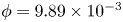$\phi = 9.89 \times 10^{-3}$, which is $2.55$ times greater than the growth rate of the nonlinear theoretical model. Similar to the $(0.8,0)$ harmonic two-dimensional waves in § 4.1, the $(2,0) = (0.4,0)$ modes in this case can experience both linear and nonlinear growth. According to linear theory, the $(0.4,0)$ modes have a growth rate of $1.01 \times 10^{-2}$, which is greater than the predicted nonlinear growth. The $(0.4,0)$ mode in figure 12 has a growth rate of $9.89 \times 10^{-3}$ until $t < 1500$, closely matching the linear growth rate. This demonstrates that the $(2,0)$ modes in the present case, despite being nonlinearly generated due to the interaction between a pair of oblique waves, experience rapid growth due to linear mechanisms. This is the case as the linear growth rate is greater than the nonlinear growth rate of these modes. It should be noted that the $(2,0)$ modes grow due to both linear and nonlinear mechanisms. However, the growth rate of the $(2,0)$ modes can be well approximated using only the linear growth rate because the linear growth rate is significantly greater than the nonlinear growth rate (see Appendix C).

The dynamics of different modes in the streamwise velocity and temperature fields at $x_1 = 0.785$ during the transition process for $(0.2,\pm 0.4)$ modes is shown in figure 13. The harmonic two-dimensional streamwise waves grow to amplitudes that are three orders of magnitude larger than streaks, which is evident at $t \sim 1500$ in figure 13. At $t \sim 1000$, the harmonic two-dimensional waves have amplitudes larger than the initial oblique waves. The plateau observed in average wall shear stress and average wall heat flux in figure 11 is due to the nonlinear saturation of the harmonic two-dimensional streamwise waves. The transition has not occurred until $t < 2300$.

Figure 13. Temporal development of $u_2$ and $\vartheta$ disturbance amplitude for different wavenumbers at a wall-normal distance $x_1 = 0.785$ at $t = 1413$. Here, $(1,1) = (0.2,\pm 0.4)$ and the rest are multiples of $(0.2,\pm 0.4)$. Thick solid black, red and blue solid lines represent the $u_2$ disturbance; thin dot-dashed black, green and magenta lines represent the $\vartheta$ disturbance.

The amplitude of the harmonic two-dimensional streamwise waves saturates at $t \sim 1500$, and at this point, there is significant energy transfer into $(0,\pm 2)$ modes. From this $t$, the streak modes grow with higher growth rates than earlier, as there is an increased energy transfer into these modes. It should be noted that similar growth rates are observed for the $(0,\pm 2)$ modes in the streamwise velocity and buoyancy fields for $(0.2,\pm 0.4)$ oblique waves, unlike the O-type transition caused by $(0.4,\pm 0.4)$ oblique waves.

Significant imbalances in energy transfer in $(3, \pm 1)$ and $(1, \pm 3)$ modes are also present, which arise from nonlinear interactions between oblique waves, harmonic two-dimensional waves and streaks (see figure 13b). As the harmonic two-dimensional waves grow much faster than the streaks, there is greater energy transfer to the $(3, \pm 1)$ modes; hence, its amplitude is around two orders of magnitude higher than $(1, \pm 3)$ modes. For the present case, linear mechanisms also aid the growth of $(3, \pm 1)$ modes initially as the oblique wave $(0.6,\pm 0.4)$ ($(0.4,0) + (0.2,\pm 0.4) = (0.6,\pm 0.4)$) lies inside the neutral curve. Again, at $t \sim 1500$, there is a significant shift in the growth of modes with now nonlinear mechanisms favouring the rapid growth of $(1, \pm 3)$ modes, which is a consequence of the rapid growth of $(0,\pm 2)$ streak modes.

The peak in figure 11 is observed at $t \sim 2400$, and it is at this point that the flow breaks down into smaller structures, and the transition has taken place. By correlating this peak to the growth of modes in figure 13, it is clear that the peak can be associated with the peak observed in the amplitude of $(0,\pm 2)$ streak mode, implying that the transition is related to the breakdown of streaks or streamwise vortex modes.

Similar to the transition observed for $(0.4,\pm 0.4)$ oblique waves, modes that are not direct descendants of the nonlinear wave–wave interactions are observed, which is a consequence of limited machine precision (Mayer et al. Reference Mayer, Von Terzi and Fasel2011). The dynamics of these modes and their interaction with the initial oblique waves are shown in figure 13(c,d). Such transition is also observed during the oblique-mode breakdown of $(0.2,\pm 0.1)$, $(0.2, \pm 0.2)$, $(0.3,\pm 0.5)$ oblique waves (not shown for brevity).

The flow field at two different wall-normal locations at $t = 1413$ is shown in figure 14. The amplitudes of the nonlinearly generated modes are nonnegligible at this time. The streamwise velocity and reduced temperature fields are correlated. Both fields exhibit flow structures resembling two-dimensional waves, demonstrating that the initial stages of transition are dominated by two-dimensional waves for these streamwise and spanwise wavenumbers. Two-dimensional waves are also observed close to the wall, unlike streaks which are only dominant away from the wall (see figure 8).

Figure 14. Flow field at $t = 1413.6$ when perturbed by $(0.2,\pm 0.4)$ oblique waves. (a) Streamwise velocity field; (b) buoyancy field at $x_1 = 0.785$; (c) streamwise velocity field (d) buoyancy field at $x_1 = 0.28$. Two-dimensional waves are present close to the wall and away from the wall. Note that the contour magnitude is different in the figures.

Therefore, a pair of oblique waves with small amplitude can cause a supercritical transition in the vertical buoyancy layer by forming streaks or harmonic two-dimensional streamwise waves during the early stages of transition. In the transition caused by $(0.2,\pm 0.4)$ oblique waves, the oblique waves nonlinearly interact with each other to generate $(0.4,0)$ two-dimensional waves, and these waves linearly can grow with $\phi = 1.011 \times 10^{-2}$. However, in the O-type transition initiated by $(0.4,\pm 0.4)$ oblique waves, the nonlinearly generated $(0.8,0)$ two-dimensional waves can linearly grow with $\phi = 3.432 \times 10^{-3}$. In both cases, the nonlinear effects aid the formation of two-dimensional streamwise waves. However, for $(0.2,\pm 0.4)$ oblique waves, the nonlinear growth of the two-dimensional waves is aided by the strong linear growth (the linear growth of $(0.8,0)$ modes is around an order of magnitude larger than the linear growth of $(0.4,0)$ modes) during the early stages of transition. Hence, two-dimensional streamwise waves dominate the early stages of transition initiated by $(0.2,\pm 0.4)$ oblique waves, unlike the O-type transition initiated by $(0.4,\pm 0.4)$ oblique waves. It should be noted that the nonlinearly generated streak modes do not experience linear growth as these modes are always linearly stable (Xiong & Tao Reference Xiong and Tao2017).

This demonstrates that two-dimensional streamwise waves can dominate the flow field during the early stages of the O-type transition of the vertical buoyancy layer if the growth of the nonlinearly generated modes is aided by the strong linear growth of the corresponding modes. This is in stark contrast to the O-type transition commonly reported in incompressible and compressible flat-plate boundary layer flows, where streaks always seem to dominate the flow (Berlin et al. Reference Berlin, Lundbladh and Henningson1994, Reference Berlin, Wiegel and Henningson1999; Chang & Malik Reference Chang and Malik1994; Mayer et al. Reference Mayer, Von Terzi and Fasel2011; Levin et al. Reference Levin, Davidsson and Henningson2005). Despite this, in both cases, the transition is related to the breakdown of streak modes in the late stages.

At $Re = 200$, streamwise vortices and streaks dominate the early transition if the initial oblique waves have relatively large streamwise wavenumbers (streamwise wavenumbers towards the right of the neutral curve in figure 3a). However, harmonic two-dimensional streamwise waves primarily dominate the flow field during the early stages of transition if the initial oblique waves have relatively small streamwise wavenumbers (streamwise wavenumbers towards the left of the neutral curve in figure 3a). This is the case as after the initial nonlinear interactions, oblique waves having low streamwise wavenumbers produce harmonic two-dimensional streamwise waves that are linearly unstable with substantial growth rates, which aid in the rapid growth of nonlinear modes.

Although a pair of oblique waves initiate the transition, some of the stages of this transition route are qualitatively similar to the H-type transition observed in several other flat plate boundary layer flows (Kachanov & Levchenko Reference Kachanov and Levchenko1984; Berlin et al. Reference Berlin, Lundbladh and Henningson1994, Reference Berlin, Wiegel and Henningson1999; Sayadi et al. Reference Sayadi, Hamman and Moin2013). In the classical H-type transition, a two-dimensional wave having streamwise wavenumber $2 \alpha$ nonlinearly interacts with three-dimensional oblique waves $(\alpha,\pm \beta )$ to form staggered $\varLambda$ vortices and cause a transition. This is the case as similar nonlinear interactions between a two-dimensional wave with streamwise wavenumber $2 \alpha$ and three-dimensional oblique waves with wavenumbers $(\alpha,\pm \beta )$ exist during the O-type transition. The similarity between H-type and O-type transition was also observed in the Blasius boundary layer (Berlin et al. Reference Berlin, Wiegel and Henningson1999).

4.2.1. Secondary flow when two-dimensional waves dominate transition

The mean spanwise velocity at different time instants is shown in figure 15. The spanwise velocity is averaged along the entire streamwise length of the domain across an $x_1$–$x_3$ plane. Similar to figure 9, only one spanwise wavelength of the initial oblique wave $2 {\rm \pi}/ \beta$ is shown. Initially, a double longitudinal vortex system (the mean spanwise velocity changes sign three times) with minimal magnitude is present. However, at $t = 2200$, there is a single longitudinal vortex system (the mean spanwise velocity changes sign two times) whose magnitude is similar to the single longitudinal vortex system shown in figure 9. At this time, the amplitude of the streak modes is greater than the amplitude of the two-dimensional waves. At $t = 2400$, an additional vortex system is present. The inner vortex system is observed in the inner boundary layer, the intermediate vortex is observed in the outer boundary layer, and the outer vortex system extends into the bulk, similar to the vortex system in figure 9(d). Similar to the secondary flows observed when streaks dominated the flow, these secondary flows also promote mixing. The spanwise wavenumber of the vortex system is again twice the wavenumber of the oblique wave. Interestingly, it is similar to the H-type transition vortex system observed in unstratified spatially developing vertical natural convection boundary layers (Zhao et al. Reference Zhao, Lei and Patterson2017), implying similarities between H-type and O-type transitions of NCBLs.

Figure 15. Mean spanwise velocity at different times during the transition initiated by $(0.2,\pm 0.4)$ oblique waves showing the presence of a longitudinal vortex system. The spanwise velocity field averaged along the entire streamwise length of the domain across an $x_1$–$x_3$ plane is represented using $\widetilde {u_3}$; (a) $t = 1800$, (b) $t = 2000$, (c) $t = 2200$, (d) $t = 2400$.