2. Mathematical model

The mathematical model for the liquid flow is standard and consists of the condition of incompressibility

(2.1)\begin{equation} {\boldsymbol{\nabla}} \boldsymbol{\cdot} {\boldsymbol{u}} = 0, \end{equation}

with ${\boldsymbol {u}}$ the liquid velocity field, and of the Navier–Stokes momentum equation

(2.2)\begin{equation} \partial_t {\boldsymbol{u}} + {\boldsymbol{u}} \boldsymbol{\cdot} \boldsymbol{\nabla}\boldsymbol{u} = -\frac{1}{\rho}{{\boldsymbol{\nabla}}} p + \nu \nabla^{2} \boldsymbol{u} + {\boldsymbol{g}}, \end{equation}

with $p$ the pressure relative to the gas pressure, $\rho$ and $\nu$ the (constant) density and kinematic viscosity of the liquid and ${\boldsymbol {g}}$ the acceleration of gravity. Following a common approach in the literature, we limit ourselves to two space dimensions, $x$ along the flow direction and $z$ normal to the plate. Even though three-dimensional waves are known to eventually develop in nominally two-dimensional settings, much of the theoretical knowledge available today is the result of studies based on the two-dimensional approximation (see, e.g. Chang & Demekhin Reference Chang and Demekhin2002; Kalliadasis et al. Reference Kalliadasis, Ruyer-Quil, Scheid and Velarde2012). This approach has led to the understanding of several basic features of the phenomenon in a simpler setting and, furthermore, its results are applicable also when three-dimensional structures develop, provided they have a slow lateral variation. The development length for three-dimensional features depends not only on parameters such as the Reynolds number, the plate inclination and the type and level of inlet disturbances, but also on the experimental set-up, e.g. films falling inside a tube (see, e.g. Park et al. Reference Park, Nosoko, Gima and Ro2004) or on a smooth or rough flat plate with lateral boundaries (see, e.g. Leontidis et al. Reference Leontidis, Vatteville, Vlachogiannis, Andritsos and Bontozoglou2010). For this reason, it is difficult to find unequivocal information in the literature where three-dimensional development lengths as short as 0.15–0.2 m (Park & Nosoko Reference Park and Nosoko2003) or as long as 1 m (Roberts & Chang Reference Roberts and Chang2000) can be found. Although most of the important conclusions of the present paper are obtained focusing on film lengths which, when converted to dimensional form with the physical properties of water, extend for 0.1 to 0.2 m, in order to provide a more complete picture, in some cases we extend the simulations over longer distances.

We assume a negligible gas flow on the free surface of the liquid film. Thus, on the basis of the orders-of-magnitude difference between the dynamic viscosity of gases and liquids, we take the tangential stress on the liquid side of the film to vanish while the normal stress balances the effect of surface tension:

(2.3)\begin{equation} -p + {\boldsymbol{n}} \boldsymbol{\cdot} {\boldsymbol{\tau}} \boldsymbol{\cdot} {\boldsymbol{n}} = -\sigma {\boldsymbol{\nabla}} \boldsymbol{\cdot}{\boldsymbol{n}}. \end{equation}

Here $\boldsymbol {n}$ is the unit normal out of the liquid domain, $\sigma$ is the surface tension coefficient and ${\boldsymbol {\tau }} = \rho \nu ({\boldsymbol {\nabla }\boldsymbol {u}} + {\boldsymbol {\nabla }\boldsymbol {u}}^{T} )$ is the viscous stress tensor. The free surface is located at $z=h(x,t)$ and is governed by the kinematic boundary condition

(2.4)\begin{equation} \partial_t h = w - u \partial_x h , \end{equation}

where $(u,w) \equiv \boldsymbol {u}$ are the two components of the liquid velocity. We impose the no-slip conditions on the solid surface and, on the remaining surfaces of the computational domain, we impose periodicity boundary conditions.

To model the scalar transfer process, we solve the convection-diffusion equation

(2.5)\begin{equation} \partial_t c + \boldsymbol{u} \boldsymbol{\cdot} {\boldsymbol{\nabla}} c = D \nabla^{2} c, \end{equation}

with $D$ the mass diffusivity and $c$ the mass concentration. We set $c=c_0$ at the inlet of the computational domain, downstream of which the surface concentration of the film is set to $c=c_i$, with $c_i$ a constant interfacial value. The associated normal flux vanishes on the solid surface, which is appropriate for a plate impervious to the solute. At the downstream boundary we use a linear extrapolation to two ghost nodes outside the computational domain writing $c_{N+1}=2c_N-c_{N-1}$ and $c_{N+2}=2c_{N+1}-c_N$, in which $c_N$ is the value of the concentration at the last grid node and $c_{N+1}$ and $c_{N+2}$ the extrapolated values. In any event, the treatment of the outlet boundary is not of particular importance, as the liquid flows out of the downstream boundary for most of the time, with back flow only during the very short time periods during which the capillary waves are near the outlet. Therefore, numerical errors introduced by the boundary condition are flushed out of the domain. In consideration of these brief periods of back flow, the sampling points we use for calculation and presentation are far upstream of the outlet to prevent possible contamination from the outlet neighbourhood.

We solve an initial-value problem starting with $c=c_0$ throughout the computational domain except for the free surface where $c=c_i$. We monitor the integrals of the mass transfer quantities over successive wave periods until steady spatial distributions are reached. From this point on every quantity attains the same value at the same position once every wave period. All the results reported in this paper are based on the steady state.

Aside from the inclination angle of the plate, which is taken to be $90^{\circ }$ in this paper, the fluid mechanics of the problem has five control parameters: one is the acceleration of gravity in the direction of the flow $g$, two refer to the liquid physical properties, $\nu$ and $\sigma /\rho$, and one is the volume flow rate $q$ of the liquid per unit length in the transverse direction. In a laboratory setting in which the film is subject to an inlet disturbance, a situation commonly referred to as an open system, a fifth parameter is the period $T$ of the disturbance. Here we prescribe instead the wavelength $\lambda$ thus placing ourselves in a so-called closed system. The two systems are related by $\lambda = u_w T$, with $u_w$ the velocity of the wave. With these parameters one can form three dimensionless groups, which may be taken to be the Kapitza and Reynolds numbers,

(2.6a,b)\begin{equation} Ka = \frac{\sigma}{\rho g^{1/3}\nu^{4/3}} , \quad Re=\frac{q}{\nu} , \end{equation}

and the ratio of the wavelength to the Nusselt film thickness

(2.7)\begin{equation} \varPi = \frac{\lambda}{h_{Nu}} ,\quad \textrm{with} \ h_{Nu} = \left(\frac{3q\nu}{g}\right)^{1/3} . \end{equation}

The form of these quantities assumes a vertical plate, which is the case to which the present study refers.

Table 1 lists the parameter values for the cases that we have simulated and on which we base our conclusions. The parameter $\delta$, originally introduced by Shkadov (see, e.g. Chang & Demekhin Reference Chang and Demekhin2002; Kalliadasis et al. Reference Kalliadasis, Ruyer-Quil, Scheid and Velarde2012; Denner et al. Reference Denner, Charogiannis, Pradas, Markides, van Wachem and Kalliadasis2018), is defined by

(2.8)\begin{equation} \delta=\frac{(3\,Re)^{11/9}}{ Ka^{1/3}} . \end{equation}

This is an important quantity because, in the limit of the boundary layer approximation, the dependence of the results on $Re$ and $Ka$ collapses into a dependence upon this single parameter. We have found, however, that the performance of the correlations (7.2) and (8.4) developed later in §§ 7 and 8 improves by allowing a separate dependence on $Re$ and $Ka$, even though the ratio of their exponents is close to that implied by (2.8). The table also shows the equivalent Strouhal number defined by

(2.9)\begin{equation} St= \frac{(u_w/\lambda)h_{Nu}}{u_{Nu}} . \end{equation}

Table 1. The table shows the parameter values for the simulations carried out in the course of the present study. The Reynolds $Re$ and Kapitza $Ka$ numbers are defined in (2.6a,b), the dimensionless wavelength $\varPi =\lambda /h_{Nu}$ in (2.7), the Shkadov parameter $\delta$ in (2.8), the Nusselt film thickness in (2.7) and the Strouhal number in (2.9); $h_m$, $h_{min}$ and $h_{eff}$ are the computed mean, minimum and effective film thicknesses (3.4a,b), (8.2) and (9.1), $u_{max}$ is the computed maximum liquid velocity, $u_w$ is the wave velocity, $u_m$ is the liquid mean velocity defined in (3.4a,b), $u_{Nu}$ is the velocity (4.2) of the Nusselt theory and $Sh_\infty$ is the numerically calculated value of the asymptotic Sherwood number. For cases 3, 5 and 12 either no asymptotic state was reached in the computational domain or the asymptotic value was strongly dependent on the Schmidt number.

3. Some theoretical considerations

In view of the liquid incompressibility, the term $\boldsymbol {u}\boldsymbol {\cdot } \boldsymbol {\nabla }c$ in (2.5) can be written as $\boldsymbol {\nabla } \boldsymbol {\cdot }(\boldsymbol {u} c)$. With this step, upon integrating the convection-diffusion equation (2.5) over the liquid volume enclosed between two adjacent surfaces perpendicular to the wall, located at $x$ and $x+\textrm {d}x$, and dividing by $\textrm {d}x$, we find that

(3.1)\begin{equation} \partial_t\int_0^{h(x,t)} c\,\textrm{d}z + \partial_x \int_0^{h(x,t)} c u\, \textrm{d}z = D \partial_x\int_0^{h(x,t)} \partial_x c \,\textrm{d}z -\dot{m} , \end{equation}

with

(3.2)\begin{equation} \dot{m}= -D \boldsymbol{n}\boldsymbol{\cdot} \boldsymbol{\nabla} c \, \frac{\textrm{d}s}{\textrm{d}x} . \end{equation}

In deriving (3.1) we have used the kinematic condition (2.4); $\textrm {d}s =\sqrt {1+(\partial _xh)^{2}}\,\textrm {d}x$ is the arc length of the interface cut by the two surfaces at $x$ and $x+\textrm {d}x$. The characteristic length for the horizontal gradient is at least the wavelength, which is much larger than the film thickness. This circumstance, coupled with the large value of the Schmidt number, justifies the neglect of streamwise diffusion (first term on the right-hand side).

As already noted, we envisage a system of waves with, in the laboratory frame, a temporal period $T$ at any fixed position $x$, and a corresponding spatial period $\lambda = u_wT$ in the wave rest frame. The time-average volume flow rate per unit transverse length in the film is given by

(3.3)\begin{equation} q = \frac{1}{T} \int_t^{t+T} \textrm{d}t \int_0^{h(x,t)} u (x,z,t)\,\textrm{d}z . \end{equation}

In view of the temporal (or spatial) periodicity, $q$ is independent of time and position along the plate. The average film thickness $h_m$ and velocity $u_m$ are defined by

(3.4a,b)\begin{equation} h_m = \frac{1}{T} \int_t^{t+T} h(x,t) \,\textrm{d}t , \quad u_m = \frac{q}{h_m}. \end{equation}

We define a local time-averaged mass flux out of the film per unit plate length by

(3.5)\begin{equation} \dot{M} = \frac{1}{T} \int_t^{t+T} \dot{m} \, \textrm{d}t = -\frac{D}{T} \int_t^{t+T} \boldsymbol{n}\boldsymbol{\cdot} \boldsymbol{\nabla} c \, \frac{\textrm{d}s}{\textrm{d}x} \, \textrm{d}t , \end{equation}

and a local time- and thickness-averaged solute concentration $c_m(x)$ in the film by

(3.6)\begin{equation} q [c_m(x)-c_i] = \frac{1}{T} \int_t^{t+T} \textrm{d}t \int_0^{h(x,t)} u (c-c_i) \,\textrm{d}z . \end{equation}

In a sense, this quantity may be considered as analogous to what is usually referred to as ‘mixing-cup concentration’ in steady conditions. In the present time-dependent problem it is not possible to define the precise instantaneous analog of that quantity because the local instantaneous flow rate may vanish. In terms of these quantities, upon averaging (3.1) over time, we find the time-averaged local relation

(3.7)\begin{equation} q \partial_x c_m = - \dot{M} . \end{equation}

With the introduction of a time-averaged mass transfer coefficient

(3.8)\begin{equation} K_m = \frac{\dot{M}}{c_m-c_i} , \end{equation}

(3.7) can be integrated formally to find that

(3.9)\begin{equation} \frac{c_m(x)-c_i}{c_0-c_i} = \exp \left(-\frac{1}{q}\int_0^{x} K_m \,\textrm{d}x \right) . \end{equation}

Upon introducing the time-averaged local Sherwood number according to

(3.10)\begin{equation} Sh = \frac{\dot{M} h_{Nu}}{(c_m-c_i)D} =\frac{K_m h_{Nu}}{D} , \end{equation}

in which $h_{Nu}$ is the film thickness of the Nusselt theory given in (2.7), the previous relation may be written in dimensionless form as

(3.11)\begin{equation} c_m^{*}(x) = \frac{c_m(x)-c_i}{c_0-c_i}= \exp \left(-\frac{1}{Pe} \int_0^{x^{*}} Sh\,\textrm{d}x^{*} \right) , \end{equation}

in which $x^{*}=x/h_{Nu}$, and the Péclet number is defined by

(3.12)\begin{equation} Pe = \frac{q}{D} . \end{equation}

Equation (3.11) can be rearranged to express the running average of the Sherwood number, $\langle Sh\rangle$ in terms of $c_m^{*}$:

(3.13)\begin{equation} \langle Sh\rangle(x)\equiv \frac{1}{x}\int_0^{x} Sh\,\textrm{d}x= - \frac{\log c_m^{*}(x) }{ x/(h_{Nu}Pe)} . \end{equation}

At this point, (3.11) and (3.13) are purely formal as the Sherwood number, in general, will depend on the Kapitza and Reynolds numbers and $\varPi$ to account for the effects of the fluid mechanics of the problem on the diffusion process, and on the Schmidt number $Sc=\nu /D$ for the diffusion itself.

4. Flat film

For future reference it is useful to briefly review some aspects of mass transfer from a flat film. The theory for a film of large thickness is textbook material and can be found, e.g. in Bird, Stewart & Lightfoot (Reference Bird, Stewart and Lightfoot2007). If the free surface of the film is placed at the position $z=h_{Nu}$, the concentration field may be written as

(4.1)\begin{equation} \frac{c-c_i}{c_0-c_i}=\textrm{erf} \left(\frac{h_{Nu}-z}{\sqrt{8Dx/3u_{Nu}}} \right) , \end{equation}

where

(4.2)\begin{equation} u_{Nu}= \frac{h_{Nu}^{2}g}{3\nu} \end{equation}

is the mean liquid velocity according to Nusselt's theory. For a flat film, $h_{Nu}$ equals the mean value of the film thickness. The average concentration calculated according to (3.6) is found to be

(4.3)\begin{equation} \frac{c_m-c_i}{c_0-c_i} =\textrm{erf}(\zeta) + \frac{1}{2\zeta\sqrt{\rm \pi}} \left[ (1-\textrm{e}^{-\zeta^{2}}) \left(\frac{1}{\zeta^{2} }-3\right) - \textrm{e}^{-\zeta^{2}}\right] , \end{equation}

with $\zeta = \sqrt {3 h_{Nu} u_{Nu}/[8D(x/h_{Nu})]} = \sqrt {\frac {3}{8} Pe/(x/h_{Nu})}$. For large $x$ this is

(4.4)\begin{equation} \frac{c_m-c_i}{c_0-c_i}\simeq \frac{3}{4\sqrt{\rm \pi}}\zeta= \frac{3}{8}\sqrt{\frac{3h_{Nu}u_{Nu}}{2{\rm \pi} D (x/h_{Nu})}} . \end{equation}

For a flat film, the instantaneous mass flux (3.2) equals the local, time-averaged mass flux, $\dot {m}=\dot {M}$, and is given by

(4.5)\begin{equation} \dot{M}=\sqrt{\frac{3Du_{Nu}}{2{\rm \pi} x}} . \end{equation}

The Sherwood number (3.10) becomes

(4.6)\begin{equation} Sh(x)=\frac{4\zeta^{2}}{2\sqrt{\rm \pi}\zeta \,\textrm{erf}(\zeta) + (1-\textrm{e}^{-\zeta^{2}}) \left(\dfrac{1}{\zeta^{2} }-3\right) - \textrm{e}^{-\zeta^{2}}} , \end{equation}

with the asymptotic limit

(4.7)\begin{equation} Sh_\infty=\frac{8}{3} \simeq 2.667 . \end{equation}

For a film with a finite thickness, the asymptotic value of the Sherwood number was calculated by Pigford (see, e.g. van Baten & Krishna Reference van Baten and Krishna2004) who found the value $Sh_\infty \simeq 3.41$. The transient (4.6) equals this value for

(4.8)\begin{equation} \frac{x}{h_{Nu}} \simeq 0.134\,Pe , \end{equation}

which can be taken as an estimate of the transition from developing to fully developed conditions.

In the following we will show the running average of the Sherwood number for the wavy film. For purposes of comparison, the dashed lines in those figures show the same quantity for the flat film with the same flow rate.

5. Numerical method

The numerical method is based on a finite-difference discretization with co-located variables except that, following Yang & Shen (Reference Yang and Shen2011), the $z$-velocity component is staggered in the direction $z$ normal to the wall. In order to deal with the grid motion due to the time-dependent free-surface profile, in the $z$ direction we use a stretched coordinate $Z$ defined by $Z = z / h(x,t)$, with $h(x,t)$ the local instantaneous film thickness; $Z = 0$ at the solid wall while $Z=1$ at the free surface.

The second-order Crank–Nicolson method is used for time discretization. The convection terms in (2.2), however, are updated in time with the second-order Adams–Bashforth scheme, as in Yang & Shen (Reference Yang and Shen2011). For the spatial discretization, the second-order central-difference scheme is used for the equations of liquid flow whereas, for the convection-diffusion equation (2.5), a third-order upwind-biased finite-difference scheme, useful for the suppression of spurious oscillations where the gradient of the concentration is large, is applied in the streamwise direction.

A standard projection method (Kim & Moin Reference Kim and Moin1985; Ferziger & Perić Reference Ferziger and Perić2002) is used to deal with the pressure-velocity coupling in (2.1) and (2.2). The continuity and momentum equations are then solved together with the kinematic condition (2.4) iteratively for convergence of the whole flow system at each time step. We solve the initial-value problem for the fluid prescribing periodicity conditions in the flow direction $x$ running the code until a steady regime is reached, with a wave of permanent form exiting the computational domain on the downstream (right) side and re-entering it on the upstream side. The code is capable of three-dimensional calculations but, in this work, the initialization is two-dimensional and no spontaneous perturbation in the third dimension develops.

The wave and flow fields found at steady state are taken as the basis for the mass transfer process. This treatment is justified by the approximation that the solute distribution in the liquid has negligible influence on the flow field, which is a reasonable assumption in many practical situations. In this way, we are able to simulate the flow field for a single spatial period and then ‘glued together’ many copies of it to extend the solution over a sufficiently long downstream distance. This procedure is necessary as, unlike the flow, the mass transfer process is not periodic in space. This procedure saves a considerable amount of computational time compared with solving the flow field and scalar transfer simultaneously.

A straightforward way to implement this idea would be to store all the information contained in a one-wavelength-long domain during one time period, and then duplicate it in both space and time. However, at each time step, this procedure would require a large number of repeated assignments and would therefore not be very efficient. The same result can be obtained in a more efficient way as follows.

We choose an integration time step for the diffusion equation given by $\delta t = \delta x/u_w$, in which $\delta x=\frac {1}{4}{\rm \Delta} x$ equals one fourth of the streamwise spatial step ${\rm \Delta} x$ used in the fluid mechanic calculation and $u_w$ is the calculated wave speed. The factor of $\frac {1}{4}$ is introduced to satisfy the Courant–Friedrichs–Lewy condition. Thus, during one $\delta t$, the wave travels a distance equal to one fourth of the flow spatial step. The use of intermediate positions $x_a\equiv x_i$, $x_b=x_i+\delta x$, $x_c=x_i+2\delta x$ and $x_d=x_i+3\delta x$ requires interpolation of the flow fields which is effected with third-order accuracy by following the Lagrangian interpolation procedure which leads to setting

(5.1)\begin{equation} \left| \begin{matrix} \psi_a \\ \psi_b \\ \psi_c \\ \psi_d \end{matrix} \right| = \frac{1}{128} \left| \begin{matrix} 0 & 128 & 0 & 0\\ -7 & 105 & 35 & -5 \\ -8 & 72 & 72 & -8 \\ -5 & 35 & 105 & -7 \end{matrix} \right| \, \left| \begin{matrix} \psi_{i-1} \\ \psi_i \\ \psi_{i+1} \\ \psi_{i+2} \end{matrix} \right| , \end{equation}

in which $\psi$ is any generic flow or geometric quantity (velocity component, interface position, Jacobian of the transformation from $z$ to $Z$).

By the definition of $\delta t$, we have a discrete time–space mapping:

(5.2)\begin{equation} \psi[{i}\,{\rm \Delta} x; t_0 + m\delta t] = \psi [(4{i}-m)\delta x; t_0] , \end{equation}

in which $i$ and $m$ are integers. Thus, only one saved snapshot of the flow field at an arbitrarily chosen time $t = t_0$ is needed to reconstruct the history of the flow quantity $\psi$ in a discrete manner. At each time step we adjust the $x$-indices of each node of the computational grid used for the diffusion calculation by using periodicity and replacing (5.2) by

(5.3)\begin{equation} \psi[{i}\,{\rm \Delta} x; t_0 + m\delta t] = \psi [I\delta x; t_0] , \end{equation}

with

(5.4)\begin{equation} I = [(\ell N_x+4i-m-1) \,\textrm{mod} \, N_x]+1 , \end{equation}

in which $N_x$ is the number of nodes in the finer grid, mod is the modulo operation and $\ell$ is an integer that renders the quantity in parentheses positive. With this index mapping, information on the flow field at the same relative position of the snapshot is available at the same memory location avoiding repeated assignment operations and memory use.

The mesh lengths were kept constant in the $x$ and $Z$ directions, with the cell length in the $x$ direction typically about 10 times larger than that in the $Z$ direction. We typically used 300 and 35 cells in the streamwise and wall-normal directions, respectively, for the fluid mechanics calculation. The resolution of the thin film regions achieved in this way is superior to that of other studies in which the volume-of-fluid method required a time-independent grid size irrespective of the local film thickness. For the diffusion equation, we carried out grid convergence studies for the various Schmidt numbers. For example, for case 0 and $Sc$ 1000, we used 35, 69, 103 and 137 cells observing negligible differences between the two finest grids even for the smallest value of $x/h_{Nu}$ shown in our figures, a region in which the boundary layer is very thin, which amounts to about 10 % of the first wavelength. The results presented below have been obtained with 103 cells. Analogous studies showed that 35, 52 and 69 cells gave an adequate resolution for $Sc = 100$, 200 and 500, respectively. The other cases were treated in a similar way. The velocity and Jacobian fields were quadratically interpolated from the three closest points onto the finer grids used for diffusion. Thus, on the basis of our own experience and of information in the literature (see, e.g. Albert et al. Reference Albert, Marschall and Bothe2014; Denner et al. Reference Denner, Charogiannis, Pradas, Markides, van Wachem and Kalliadasis2018) we are confident to have a good spatial resolution. The time step was conservatively set on the basis of standard stability conditions.

6. Validation

We compare in figure 1 the results of our simulations with those reported by Dietze et al. (Reference Dietze, Al-Sibai and Kneer2009). The pertinent parameter values are given in the first line of table 2; for inclined plates, the proper definition of the Kapitza number is

(6.1)\begin{equation} Ka =\frac{\sigma}{\rho (g\sin\theta)^{1/3}\nu^{4/3}} . \end{equation}

Figure 1. The open circles show the measured film height (a) and streamwise velocity at a distance of 120 ${\rm \mu}$m from the wall (b) reported by Dietze et al. (Reference Dietze, Al-Sibai and Kneer2009). The solid lines are the results of the present simulations and the barely distinguishable dotted lines are the numerical results of Dietze (Reference Dietze2016). The pertinent parameter values are shown in the first line of table 2.

Table 2. Parameter values for the waves of figures 1 and 2 used to validate the present simulations. The Reynolds $Re$ and Kapitza $Ka$ numbers are defined in (2.6a,b) and (6.1); $\lambda$ is the wavelength, $h_{Nu}$ the Nusselt film thickness (2.7) and $\theta$ the inclination angle of the plate. The last column gives the figure number in the original reference shown in the next-to-last column.

The open circles in the figure are the film height (a) and streamwise velocity at a distance of $120\ \mathrm {{\rm \mu} }\textrm {m}$ from the wall (b) reported in the reference. The solid lines are our simulations and the barely distinguishable dotted lines under it the numerical results of Dietze (Reference Dietze2016). In order to show this comparison we have converted our results from space to time using the computed phase velocity. As can be seen, the two computations are virtually identical and both closely match the data.

For another comparison we turn to the study by Denner et al. (Reference Denner, Charogiannis, Pradas, Markides, van Wachem and Kalliadasis2018). The black dots in figure 2 show the measured film heights (top row) and free-surface streamwise velocity (bottom row) reported in the reference; our numerical results are shown by the solid lines. The mean film thicknesses $h_m$ used in our simulations was deduced from the values of $Re$ and $Ka$ given by Denner et al. (Reference Denner, Charogiannis, Pradas, Markides, van Wachem and Kalliadasis2018); the wavelength $\lambda$ was measured from the graphs in the reference except for the cases which do not include more than one full wave which, therefore, we cannot simulate. Once again, the comparison is very good and shows the reliability of our simulations.

Figure 2. Comparison of our simulations, shown by the solid lines, with the experimental results of Denner et al. (Reference Denner, Charogiannis, Pradas, Markides, van Wachem and Kalliadasis2018); the pertinent parameter values are given in table 2. The top row is the local film height normalized by the Nusselt value; the bottom row is the surface velocity parallel to the plate normalized by the Nusselt velocity (4.2).

Yet another comparison of our results with relations in the literature is afforded by the correlations of the wave celerity $u_w$ and peak wave height $h_p$ for film flow along a vertical surface presented in Nosoko et al. (Reference Nosoko, Yoshimura, Nagata and Oyakawa1996) which, in our notation, are

(6.2)\begin{equation} N_{uw}\equiv \frac{u_w}{(\nu g)^{1/3}}=1.27 \frac{\varPi^{0.31}Re^{0.47}}{Ka^{0.06}} , \end{equation}

and

(6.3)\begin{equation} N_{hp}\equiv \left(\frac{g}{\nu^{2}}\right)^{1/3}h_p = 0.565 \frac{\varPi^{0.39}Re^{0.59}} {Ka^{0.132}} . \end{equation}

The two plots of figure 3 compare our computational results with these correlations. It is seen that the computed points fall very close to the values predicted by the correlations.

Figure 3. Comparison of the present computational results (open squares) with the correlations (6.2) for the wave celerity $u_w$ and (6.3) for the peak wave height $h_p$ proposed by Nosoko et al. (Reference Nosoko, Yoshimura, Nagata and Oyakawa1996).

Experiments in open systems show that, when the excitation frequency is low, disturbances evolve into multipeaked forms (see, e.g. Alekseenko, Nakoryakov & Pokusaev Reference Alekseenko, Nakoryakov and Pokusaev1985; Liu & Gollub Reference Liu and Gollub1994; Argyriadi, Serifi & Bontozoglou Reference Argyriadi, Serifi and Bontozoglou2004). It is not known what is the analog of this behaviour for closed systems, such as the ones investigated here and, in particular, whether the waveforms that we have studied are physically realizable. To gain some assurance on this aspect, we have carried out simulations in a domain twice as long as the longest one on which we report (case 5, discussed in § 7) and we have found that a second large hump emerges within the periodic domain in this case. We have also carried out a simulation mimicking an open system with the approximate model of Mudunuri & Balakotaiah (Reference Mudunuri and Balakotaiah2006) and the parameters of our case 5 finding a stable waveform and wavelength. Our base case (case 0) is based on the work of Nosoko & Miyara (Reference Nosoko and Miyara2004) and, with the exception of case 5, all other cases have a comparable or smaller wavelength, Reynolds number and Kapitza number. Thus, we are fairly confident that the waves that we study are not an artifact of our computational method but are, in fact, physically realizable.

When it comes to validation of the mass transfer component of the calculation, there is not much suitable information in the literature as the reported results are all affected by the transient nature of the developing flow. Thus, we are forced to limit ourselves to the flat-film case. The analytic solution for a film of infinite depth, given in the previous section, is suitable for comparison in the initial stage of the process, while the asymptotic value of the Sherwood number for a film with a finite thickness is suitable for the final stages of the process. Figure 4(a) shows the computed $Sh$ versus $x/(h_{Nu}Pe)$ and compares it with the short-time, infinite-depth case and long-time finite-depth one. The numerical results have been obtained with $Re = 16.1$, $Sc = 100$ and 1000, and $Re = 4.02$ and $Sc = 1000$. According to the flat-film theory of § 4, the specific values of these quantities should have no effect if $Sh$ is plotted as a function of $x/(h_{Nu}Pe)$. The three results very nearly superpose.

Figure 4. $(a)$ The (barely distinguishable) three lines which asymptote to the horizontal dashed line are the present computational results for the local Sherwood number for flat films with $Re = 16.1$, $Sc = 100$ and 1000, and for $Re = 4.02$ and $Sc = 1000$. The dashed line is the analytic result for a thick film, (4.6); the horizontal dashed line is the asymptotic result for a film with a finite thickness. $(b)$ Comparison between the correlation (6.4) for the running average of the Sherwood number defined in (3.13) and the present computational results.

As shown in figure 4(b), for the flat film, the numerical results for the running average of the Sherwood number defined in (3.13) are closely approximated by the correlation

(6.4)\begin{equation} \langle Sh\rangle=\left[3.41^{2.5} +\left(-\frac{\log c_m^{*}}{x/(h_{Nu}Pe)}\right)^{2.5} \right]^{0.4} , \end{equation}

in which $c_m^{*}$ is given by (4.3).

7. Large-wave regime

We begin the discussion of the present results focusing on what may be called the large-wave regime, in which the wave develops a recirculation region in its rest frame. The threshold for this occurrence can be identified with the condition in which the maximum liquid velocity $u_{max}$ in the absolute frame equals the velocity $u_w$ of the wave itself. The empirical correlation

(7.1)\begin{equation} \frac{u_{max}}{u_w}=0.707 \frac{\varPi^{0.0436} Re^{0.241}}{Ka^{0.0680}} , \end{equation}

based on our numerical results, provides a reasonable fit to them as can be seen in figure 5(a), which includes all the cases that we have simulated. As figure 5(b) shows, after removing the points with small values of $u_{max}/u_w$ identified by the (blue) circles in figure 5(a), a better fit is obtained with the slightly modified expression

(7.2)\begin{equation} \frac{u_{max}}{u_w}=0.661 \frac{\varPi^{0.0491} Re^{0.202}}{Ka^{0.0483}} . \end{equation}

The three cases removed to generate this correlation also show a poorer fit with the original correlation in the left plot of figure 3. We identify as large waves such that the computed value of $u_{max}/u_w$ exceeds 1. Cases for which $u_{max}/u_w\lesssim 1$ will be considered in the next section. The value $u_{max}/u_w = 1$ is introduced mostly for convenience as it is not a hard threshold. Waves for which the ratio falls slightly below or slightly above share features of both small and large waves. (It may be noted that the ratio of the exponents of $Re$ to $Ka$ in the previous correlations are 3.54 and 4.18, not too different from the ratio $11/3\simeq 3.67$ implied by the Shkadov parameter $\delta$.)

Figure 5. Comparison of the computational results with the correlation (7.1), plot (a), and (7.2), plot (b), for the ratio $u_{max}/u_w$ of the maximum flow velocity in the absolute frame to the wave velocity. Plot (a) includes the results for all the cases of table 1. Plot (b) only includes the cases with $u_{max}/u_w \gtrsim 0.9$; the circles in (a) (blue) identify the points deleted in (b).

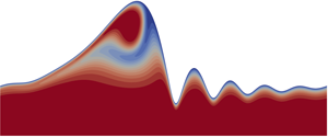
The upper frames in each row of figure 6 show the wave shape for case 0 at successive positions downstream of the inlet with the colour indicating the solute concentration; the first frame also includes the streamlines in the wave rest frame which, due to the steadiness of the flow in this frame, do not change in the course of the propagation. An animation of this sequence is available as supplementary movies at https://doi.org/10.1017/jfm.2020.587. The lower frames in each row are the corresponding normalized mass flux $\dot {m}^{*}$ defined by

(7.3)\begin{equation} \dot{m}^{*} = \frac{\dot{m}\, h_{Nu}}{(c_0-c_i)D} , \end{equation}

at the same instant of time; similar results for the mass transfer rate have been shown by Sisoev et al. (Reference Sisoev, Matar and Lawrence2005) and for the local Sherwood number by Albert et al. (Reference Albert, Marschall and Bothe2014). The horizontal axis is the dimensionless downstream distance $x/h_{Nu}$. The parameter values for this case are given in the first line of table 1.

Figure 6. Successive snapshots of the wave propagating along the plate for the conditions of case 0 of table 1. The colour is the solute concentration for $Sc =1000$. The graph under each wave shape shows the local instantaneous mass flux $\dot {m}$ at the wave surface normalized according to (7.3). The vertical scale is amplified by a factor of 25 with respect to the horizontal scale; a detail with equal scales in the two directions is shown in figure 7. The two circles are the stagnation points associated to the recirculation.

In the wave rest frame, recirculation is the result of the appearance of the two stagnation points marked in figure 6 on the right and left faces of the wave. In the laboratory frame these would be downstream and upstream faces, while they become the upstream and downstream faces, respectively, in the wave rest frame, which is the frame we use in the following discussion. We refer to the streamline joining the stagnation points as the separation streamline.

Figure 7. Snapshots of the region around the ‘whisker’ of solute-rich liquid on the back of the main crest corresponding to the last five frames of figure 6. The solid lines identify the boundary of the region where the solute concentration exceeds 50 % of the initial value. The arrows indicate the downstream end of the solute-rich ‘whisker.’ Here the vertical scale is not magnified but is equal to the horizontal scale.

The liquid in the neighbourhood of the front (right) stagnation point comes from the boundary layer on the surface of the film upstream (to the right) of the large crest and is therefore depleted of solute. Accordingly, as can be seen from the figure, the mass flux in this neighbourhood remains close to zero for all times. As noted, among others, by Yoshimura et al. (Reference Yoshimura, Nosoko and Nagata1996), Rastaturin et al. (Reference Rastaturin, Demekhin and Kalaidin2006) and Dietze (Reference Dietze2019), this liquid from the previous boundary layer is deflected under the separation streamline penetrating the large wave toward its rear face thus acquiring a velocity component normal to the interface. Interestingly, these streamlines do not reach the free surface at the back (to the left) of the wave but are deflected thus leaving a thin ‘whisker’ of relatively solute-rich fluid, particularly evident in frame (c), between themselves and the free surface on which, therefore, a new boundary layer forms; as cited in Yoshimura et al. (Reference Yoshimura, Nosoko and Nagata1996) a similar pattern was also shown in a conference contribution by Nagasaki & Hijikata (1990). Yoshimuraet al. (Reference Yoshimura, Nosoko and Nagata1996) used it to develop a double-boundary-layer model. In this way the concentration field becomes multi-layered, which is responsible for the complex features of the process.

A more detailed view of the development of this multi-layered structure is provided by figure 7, which focuses on this region using equal scales in the horizontal and vertical directions; the five images correspond to the last five frames of figure 6. The dark solid line marks the $c_m^{*}=0.5$ boundary. As long as this whisker has not been depleted, the largest mass flux occurs from the new boundary layer forming along the back of the main crest. However, it is seen from frame (e) of figure 6 onward that the mass flux from the back of the wave, after the two boundary layers merge, becomes quite comparable to that from the rest of the film except for a very small increase in the region where the recirculation brings fresh solute-reach liquid near the surface. Of course, superimposed on this fairly constant value of the mass flux are maxima and minima in correspondence of the minima and maxima of the film thickness. Indeed, from the local $\dot {m}^{*}$ shown under the wave shapes in figure 6, we observe a good correspondence between mass transfer and wave shapes in the sense that the mass flux is roughly inversely proportional to the local film thickness as remarked by several authors (see, e.g. Morioka & Kiyota Reference Morioka and Kiyota1991; Bo et al. Reference Bo, Ma, Chen and Lan2011). More than because of an inverse proportionality of $\partial c/\partial z$ to the local film thickness (or, possibly, in addition to this factor), the enhanced gradient may be due to the convergence of the streamlines under the wave troughs, clearly visible in the first frame of figure 6, since, in a large-Schmidt-number system, streamlines approximate iso-concentration lines away from the main crest.

In order to study the connection between film thickness and mass transfer rate, following Charogiannis & Markides (Reference Charogiannis and Markides2019), we show in figure 8 a graph of the dimensionless time-dependent mass transfer rate

(7.4)\begin{equation} k_m^{*}(x,t) = \frac{\dot{m}(t)h_{Nu}}{(c_m(x)-c_i)D} \end{equation}

versus the local film thickness non-dimensionalized by division by $h_{Nu}$ for three values of $x$; time runs counter-clockwise. The dashed line is the flat-film asymptotic value $Sh_\infty =3.41$ for the corresponding film thickness. The largest loop is for $x/h_{Nu} = 50$, which is close to half a wavelength from the start of the mass transfer. It shows a very large mass transfer from the freshly exposed top and back of the wave, that becomes smaller and oscillatory in the capillary-wave substrate. The intense mass transfer from the top of the wave is due to the velocity normal to the interface close to the left stagnation point mentioned before. The substrate does not benefit from a similar mechanism and the transfer rate is correspondingly smaller. At $x/h_{Nu} = 500$ (blue line), about five wavelengths downstream of the beginning of the mass transfer, there still is a fairly sustained mass flux from the top and back side of the wave, with a maximum near the left stagnation point due to the recirculating flow. The last line (violet) is for $x/h_{Nu} = 5000$. The effect of recirculation is nearly gone and the general trend is similar to, although mostly above, that of a flat film.

Figure 8. Dimensionless time-dependent mass transfer rate defined in (7.4) versus local film thickness for case 0. The large loop (red) is for $x/h_{Nu} = 50$, the intermediate one (blue) for $x/h_{Nu} = 500$ and the smallest one (violet) for $x/h_{Nu} = 5000$; the dashed line is the flat-film result.

The left plot of figure 9 shows the normalized time-averaged local mass transfer rate $\dot {M}^{*}$ versus $x/h_{Nu}$ for, in ascending order, $Sc = 100$, 200, 500 and 1000. The main features of these curves are interpreted with the help of the right plot which reproduces the line for $Sc = 500$ on a log-log scale. Initially there is a short period of rapid decrease, stage 1, similar to that for a flat film, which lasts less than one wavelength. This is followed by a near-plateau (stage 2), which is fed by the component of the convection velocity normal to the interface on the left side of the large wave. When the solute-poor liquid reaches the back of the wave forming the whisker, the mass transfer declines fairly rapidly as this structure is eroded, stage 3, and, when the whisker has completely disappeared, the decline temporarily decreases, stage 4, and then picks up speed similarly to the flat-film case as the finite thickness of the liquid layer becomes a limiting factor.

Figure 9. (a) Time-averaged local mass flux along the wave normalized in the same way as shown in (7.3) for case 0 of table 1 for, in ascending order, $Sc = 100$, 200, 500 and 1000. (b) The $Sc = 500$ line of the graph on the left illustrating the stages of the process described in the text.

If the same data were plotted as in figure 15 below by showing $Sh$ defined as in (3.10), the graph would be quite similar, the main difference being a shallow maximum corresponding to the near constant $\dot {M}$ divided by the decreasing $c_m-c_i$ in stage 2. The combination of the different physics determining these two quantities would cloud the interpretation of the Sherwood number and perhaps also its practical usefulness.

The complexity of the processes just described prevents a simple scaling of the local mass transfer rate or of the local Sherwood number. However, some useful conclusions can be derived for the running average $\langle Sh\rangle (x)$ of the Sherwood number defined in (3.13), which is presented in three different ways in figure 10. The solid lines in the first plot show $\langle Sh\rangle (x)$ for, in ascending order, $Sc = 100$, 200, 500 and 1000. The lines are nearly parallel for some distance demonstrating the influence of convection, which affects all Schmidt numbers equally. The dashed lines are the corresponding results for a flat film with the same flow rate. Initially, the curves closely follow the flat-film results. This feature is particularly clear from the central plot which shows the ratio of the running averages of the Sherwood number of the wavy to the flat film. Here, all the curves start from $\langle Sh \rangle /\langle Sh \rangle _\infty = 1$.

Figure 10. Three views of the running average $\langle Sh\rangle (x)$ of the Sherwood number defined in (3.13) for case 0 of table 1. (a) The solid lines show $\langle Sh\rangle$ for, in ascending order, $Sc = 100$, 200, 500 and 1000, while the dashed lines show the same quantity for a flat film with the same flow rate. (b) Ratio of $\langle Sh\rangle (x)$ for the wavy film to the same quantity for the flat film. (c) The Sherwood number for the wavy film normalized by $Sc^{1/3}\sqrt {\log Sc}$. The flat-film results have been obtained by numerical simulation.

A few wavelengths downstream one observes two aspects by which the results differ from the flat-film Sherwood number. The first one is a range of significantly slower decrease, the second one the settling of the curves to a nearly constant value higher than for the corresponding flat film. These features suggest the presence of two different mechanisms. The former one is due to the beneficial effect of the large wave with the solute-rich liquid deflected under the separation streamline reaching the back of the main crest as shown in figures 6 and 7. The benefit of this process, however, is temporary as explained before. The latter mechanism is due to the thinner film under the capillary wave troughs as explained later in § 8. Turning now to the middle plot, we notice that, except very near the beginning of the simulation, the ratio is above 1, exceeding 2 far from the inlet, as expected from the comparison in the left plot. The collapse of the curves in the intermediate region suggests a dominant effect of convection in the large-wave-dominated phase.

The right plot of figure 10 shows the same data for the wavy film Sherwood number represented by the solid lines in the left plot replotted in the form of $\langle Sh\rangle / Sc^{1/3}\sqrt {\log Sc}$. Division by $\sqrt {\log Sc}$ was suggested by Roberts & Chang (Reference Roberts and Chang2000) to model the effect of recirculation. It can be seen that, with this normalization, the curves nearly collapse for the first 2–3 wavelengths but diverge further downstream, implying that recirculation is important only in a short initial stage of the flow.

While the running average of the Sherwood number gives a sense of how the mass transfer rate depends on distance from the inlet, it does not tell us the rate at which the film is depleted of solute. This information is presented in figure 11, where the left plot refers to the case under consideration and the right plot to case 5 discussed later. For the present case, it appears that $\log c_m^{*}$ is very close to a straight line, except for very small $x$, suggesting an essentially constant $Sh$. However, the weight of the initial stage becomes more and more important as $Sc$ decreases due to the rapid loss of solute, thus limiting the usefulness of a constant-$Sh$ approximation. For example, for $Sc = 100$, the mean concentration is reduced to 1 % of its initial value already by $x/h_{Nu}\simeq 1200$. The constant-$Sh$ approximation becomes more useful for larger $Sc$ for which the initial transient represents a shorter fraction of the part of the process of practical interest. For $Sc = 1000$, for example, the film still retains 10 % of the initial amount of solute for $x/h_{Nu}\simeq 5000$, well into the linear region of $\log c_m^{*}$.

Figure 11. Time- and thickness-averaged solute concentration normalized as in (3.11) as a function of the normalized downstream distance; in ascending order, the curves are for $Sc = 100$, 200, 500 and 1000. Plots (a) and (b) are for cases 0 and 5 of table 1.

When the recirculation is stronger than in the case considered so far, the features we have discussed become more marked and complex. A figure similar to figure 6 for a larger wave, case 5 in table 1, is shown in figure 12 (see also the animation available as supplementary movies). The difference in the values of $u_{max}/u_w$ is less than 10 %, but significant new effects appear. The main difference that stands out is the larger mass flux from the top of the large crest caused by the stronger recirculation. However, if we look deeper and consider the running average of the Sherwood number, more differences appear.

Figure 12. Successive snapshots of the wave propagating along the plate for the conditions of case 5 of table 1. The colour is the solute concentration for $Sc =1000$. The graph under each wave shape shows the local, instantaneous mass flux $\dot {m}$ at the wave surface normalized according to (7.3). The vertical scale is amplified by a factor of 25 with respect to the horizontal scale. The two circles are the stagnation points associated to the recirculation.

The three plots of figure 13 are similar to those of figure 10. The solid lines in the first plot, corresponding, in ascending order, to $Sc = 100$, 200, 500 and 1000, are more nearly parallel over the entire range than in the previous case signifying the complete dominance of convection for any Schmidt number. In the very initial stage, $\langle Sh\rangle$ for the wavy film is slightly below that for the flat film because, due to the formation of waves, the mean velocity of the former is somewhat larger than that of the latter so that, over a given distance, the time available for transfer is less. We have carried out a specific grid convergence study to make sure that this result is not a numerical artifact. In support of this result we note that, as shown in table 1, the ratio of the Nusselt thickness to the mean thickness of the wavy film is greater than 1 which implies, for the same flow rate as considered in this comparison, a smaller velocity of the flat film. The adverse effect of a higher velocity on the transfer is also evident from (4.1) for the case of a flat film.

Figure 13. Three views of the running average $\langle Sh\rangle (x)$ of the Sherwood number defined in (3.13) for case 5 of table 1. (a) The solid lines show $\langle Sh\rangle$ for, in ascending order, $Sc = 100$, 200, 500 and 1000, while the dashed lines show the same quantity for a flat film with the same flow rate. (b) Ratio of $\langle Sh\rangle (x)$ for the wavy film to the same quantity for the flat film. (c) The Sherwood number for the wavy film normalized by $Sc^{1/3}\sqrt {\log Sc}$. As for figure 10, the flat-film results have been obtained by numerical simulation.

For larger $x/h_{Nu}$, the slope of the lines suggests that their steep descent continues beyond $x/h_{Nu} = 6000$ and, for the lower Schmidt numbers, $\langle Sh \rangle$ falls even below the corresponding lines for a flat film with the same flow rate (dashed lines). These features are an indication of a relatively inefficient diffusion process. The reason is that, while the substrate film by itself would release solute not very differently from a flat film, the rate at which this happens from the large waves is much slower due both to the recirculation and to their faster velocity (about five times that of the substrate) which reduces the time available to release solute over a given length. Due to these factors, the running average of the Sherwood number is penalized by the relatively inefficient process by which solute is released from the fraction of film occupied by the large waves. The imbalance between the solute released from the various parts of the wave, therefore, negatively affects the overall efficiency of the diffusion process.

This point is particularly clear in the right plot of figure 11 which shows $\log c_m^{*}$ versus $x$ for this case for different $Sc$. A first important difference with the previous moderate-recirculation case is the much slower rate of mass loss. For example, for $Sc = 100$, now the film has lost 99 % of its initial solute content by $x/h_{Nu}\simeq 3000$, while in the previous case this had already happened for $x/h_{Nu}\simeq 1200$. It is therefore seen that the imbalance among the rates at which the different parts of the wave lose solute causes a major loss in the mass transfer efficiency. For an equivalent open system, in which the spatial periodicity is replaced by a temporal periodicity, this conclusion suggests that a low excitation frequency would adversely affect the mass transfer operation.

The difference between the two situations is evidenced in figure 14 which compares the solute distribution in the two cases at the time when the film has lost 90 % of the initial amount of solute. While the mass flux from the wave of the previous case 0 is fairly uniformly distributed, that for the larger wave of case 5 peaks in the recirculation region and is very small everywhere else.

Figure 14. Comparison between cases C0 and C5 of table 1 of the solute concentration in the wave by the time 90 % of the solute has been lost; the Schmidt number equals 500. The vertical scales are amplified by 12.5 and 25 times in the left and right frames, respectively.

The central plot of figure 13 is the ratio of $\langle Sh \rangle$ for the wavy to the flat film. While the initial behaviour is similar to that of the previous case, one observes an eventual decline of the ratio for the lower Schmidt numbers. In addition to the reduced mass transfer from the depleted film mentioned before, this is due to the relatively large amount of solute trapped in the recirculation zone of the large wave, evident in figure 14, which increases the mean concentration $c_m^{*}$ thus depressing $\langle Sh \rangle$, as is evident from the expression (3.13) of this quantity.

Finally, the right plot of figure 13 shows $\langle Sh \rangle (x)$ normalized by division by $Sc^{1/3}\sqrt {\log Sc}$ as before. Due to the larger role played by the recirculation, the collapse of the curves extends over a much longer region than in the previous case.

As figure 15 shows, contrary to the small-wave case discussed in the next section, after the local maximum the local time-averaged Sherwood number appears to decrease continuously all the way to the end of the integration for $x/h_{Nu}\sim 6000$. It is difficult to determine numerically if this trend continues indefinitely or an asymptotic stage in which $Sh$ settles to a constant value is eventually reached. In any case, this is a rather academic point as most of the solute has left the film while $Sh$ decreases as can be seen in the right plot where $Sh(x)$ is plotted as a function of the amount of solute lost by the film at each position $x/h_{Nu}$.

Figure 15. Local Sherwood number for case 5 of table 1 versus $x/h_{Nu}$ (a) and $1-c_m^{*}$ (b). In ascending order the lines are for $Sc= 100$, 200, 500 and 1000.

8. Small-wave regime

We now turn to situations in which $u_{max}/u_w$ is less than 1 so that the main part of the wave does not exhibit a recirculation region. Figure 16 shows a typical case close to the upper range of these waves for $u_{max}/u_w$ = 0.892 (see also the animation available as supplementary movies). The lines in the lower figures show the local instantaneous normalized mass flux as previously. The depleted boundary layer reaching the top of the wave thickens due to the diverging streamlines, which further depresses the mass transfer.

Figure 16. Successive snapshots of the wave propagating along the plate for the conditions of case 11 of table 1. The colour is the solute concentration for $Sc$ = 2000. The graph under each wave shape shows the local, instantaneous mass flux $\dot {m}$ at the wave surface normalized according to (7.3). The vertical scale is amplified by a factor of 25 with respect to the horizontal scale.

Figure 17 is similar to figure 8 for case 0 and shows the time-dependent mass transfer rate $k_m^{*}(x,t)$ versus the local film thickness non-dimensionalized by division by $h_{Nu}$ for three values of $x$; time runs counter-clockwise. The dashed line is the flat-film asymptotic value $Sh_\infty =3.41$ for the corresponding film thickness. The largest loop (open circles, taken at equal time intervals) is for $x/h_{Nu} = 50$, which is close to half a wavelength from the start of the mass transfer. As can be seen in figure 16, the minimum mass transfer occurs just to the right of the peak. It then grows rapidly toward the back of the crest because this region has not yet been reached by the depleted boundary layer and due to the convergence of the streamlines. The density of points in this region indicates a strong contribution of this region. Further downstream, at $x/h_{Nu} = 200$ (blue) and $x/h_{Nu} = 2000$ (violet), the mass transfer is much smaller and closer to that for a flat film, with enhancements near the troughs and diminution near the crests corresponding to the convergence and divergence of the streamlines.

Figure 17. Dimensionless time-dependent mass transfer rate defined in (7.4) versus local film thickness for case 11. The large loop, in which the red circles are equally spaced in time, is for $x/h_{Nu} = 50$, the intermediate one (blue) for $x/h_{Nu} = 200$ and the smallest one (violet) for $x/h_{Nu} = 2000$; the dashed line is the flat-film result.

The solid lines in the left plot of figure 18 show the running average of the Sherwood number for this case for, in ascending order, $Sc= 200$, 500, 1000 and 2000 and afford a comparison with the corresponding flat-film results shown by the dashed lines. The difference between the wavy and flat films is greatly reduced in comparison with the cases of the previous section. The ratio of the wavy to flat-film Sherwood numbers is plotted as a function of $x/h_{Nu}$ in the right plot. This way of plotting the results brings them together in spite of the different Schmidt numbers. In this case, division by the flat-film result normalizes the $Sc$ dependence so that the outcome is mostly dependent on the flow field, which this figure shows to affect the mass transfer approximately equally for all Schmidt numbers. In any event, the region of rapid transition is seen to be rather short, less than two wavelengths.

Figure 18. Two views of the running average $\langle Sh\rangle (x)$ of the Sherwood number defined in (3.13) for case 11 of table 1. (a) The solid lines show $\langle Sc\rangle$ for, in ascending order, $Sc = 200$, 500, 1000 and 2000 while the dashed lines show the same quantity for a flat film with the same flow rate. (b) Ratio of $\langle Sh\rangle (x)$ for the wavy film to the same quantity for the flat film. As for figures 10 and 13, the flat-film results have been obtained by numerical simulation.

Another aspect in which these results differ from those of the large waves is that the local, time-averaged Sherwood number tends to become a constant rather than continually decreasing, much as the Nusselt number for heat transfer in laminar duct flow which is independent of the Prandtl number. This result suggests that, in fully developed conditions, diffusion occurs primarily normally to the streamlines and is little affected by convection. The point can be appreciated from figure 19. Here the left plot, showing the local, time-averaged Sherwood number, demonstrates the independence of this quantity from the Schmidt number in the asymptotic regime. This asymptotic regime is of practical importance as can be seen in the right plot, which plots $Sh$ versus $1-c_m^{*}$. It is seen here that the asymptotic regime sets in by the time the film still contains more than 75 % of the initial concentration of solute. Although a ‘whisker-like’ structure is visible in figures 16(b) and 16(c), there are significant differences with the previous cases insofar as it is thicker, the component of the velocity normal to the interface is greatly reduced and the whisker is eroded from right to left rather than left to right as is particularly evident in figure 7. (In other words, it is the side of the whisker facing the large wave that starts to disappear first rather than the left side, most distant from the large wave.) The step-like decrease of $Sh$ in the left plot (which is amplified by the use of the logarithmic scale) corresponds to the disappearance of the whisker between frames (c) and (d) of figure 16.

Figure 19. Local Sherwood number for case 11 of table 1 versus $x/h_{Nu}$ (a) and $1-c_m^{*}$ (b). In ascending order the lines are for $Sc = 200$, 500, 1000 and 2000. Note the approach to an asymptotic constant value independent of the Schmidt number.

These features are less marked for waves with an even smaller value of $u_{max}/u_w$. Figure 20 shows an example for $u_{max}/u_w = 0.726$. As in the previous case, the time average of the local Sherwood number in the left plot also tends to a common value independent of the Schmidt number, but the curves are much smoother than in the previous case and closer to the flat-film behaviour. When plotted as functions of $1-c_m^{*}$, the curves for the various $Sc$ nearly collapse (right plot).

Figure 20. Local Sherwood number for case 2 of table 1 versus $x/h_{Nu}$ (a) and $1-c_m^{*}$ (b). In ascending order the lines are for $Sc = 200$, 500, 1000 and 2000. Note the approach to an asymptotic constant value independent of the Schmidt number.

While the asymptotic time-averaged Sherwood number is independent of the Schmidt number unless the wave amplitude is large, it does depend on the flow. Our simulations suggest the validity of the approximate relation

(8.1)\begin{equation} Sh_\infty=\frac{3}{h_{min}^{*}} , \end{equation}

where $h_{min}^{*}$ is the normalized minimum film thickness. As figure 21(a) shows, for all our cases this quantity is well represented by the correlation

(8.2)\begin{equation} h_{min}^{*}=\frac{h_{min}}{h_{Nu}}=0.679\,\frac{Ka^{0.114}} {Re^{0.455}} . \end{equation}

Figure 21. (a) Comparison of the correlation (8.2) for the minimum film thickness with the present computational results; the blue triangle is from figure 22 of Dietze (Reference Dietze2016). (b) Comparison of the approximation (8.1) to the asymptotic time-average Sherwood number with the computational results.

Again we see that the ratio of the exponents of $Re$ and $Ka$ is 3.99, close to the value $11/3\simeq 3.67$ of the Shkadov scaling. However, allowing the ratio of the exponents of $Re$ and $Ka$ to be slightly different improves the performance of the correlation. As the correlation (8.2) shows, the wavelength appears to have a negligible effect on $h_{min}^{*}$, which perhaps implies a similarly small effect of the excitation frequency in an open system. From the definition (3.10) of the Sherwood number, we see that (8.1) is in fact equivalent to $Sh'_\infty =3$, with $Sh_\infty '=\dot {M} h_{min}/(c_m-c_i)D$. The performance of the relation (8.1) is shown in figure 21(b). As already noted, the importance of the film thinning may be related more to the convergence of the streamlines (which approximate iso-concentration lines) under the wave troughs than to the reduced thickness itself. The situation would be different for smaller values of $Sc$ (or $Pr$ for heat transfer), for which the film thickness becomes the dominant length scale as can be seen, e.g. in figure 12 of Miyara (Reference Miyara1999).

Another way to correlate $Sh_\infty$ directly with the three governing parameters is, in this small-wave case,

(8.3)\begin{equation} Sh_\infty = 4.01 \frac{\varPi^{0.0669}Re^{0.450} } {Ka^{0.144}} . \end{equation}

The performance of this correlation is shown in the left plot of figure 22. Since the transition from small to large waves is not sharp, but gradual, an asymptotic value for $Sh_\infty$ also exists for waves with $u_{max}/u_w$ close to 1. In this case, however, one observes a weak dependence of the asymptotic value on the Schmidt number (e.g. about 3.3 % between $Sc$ = 100 and 1000 for case 0). The values listed in table 1 and shown in figures 21(b) and 22(b) for these cases are averages over the computed results for four Schmidt numbers. With the inclusion of these averaged values, the previous correlation is slightly modified to

(8.4)\begin{equation} Sh_\infty = 3.51 \frac{\varPi^{0.113} Re^{0.562}} {Ka^{0.182}} , \end{equation}

although, as the right plot of figure 22 shows, the fit is not as good as including only the smaller waves. The ratios of the exponents of $Re$ and $Ka$ in these two correlations are 3.13 and 3.09, respectively, also close to the Shkadov scaling which was developed for the flow rather than the mass transfer features. The approximately similar scaling suggests a significant effect of the flow on the asymptotic Sherwood number.

Figure 22. Comparison of the correlations (8.3) (a) and (8.4) (b) for the asymptotic Sherwood number with the computational results. The uppermost points in (b) (blue circles) are the four cases of table 1 with $0.998\leq u_{max}/u_w\leq 1.044$.

9. Summary and conclusions

We have described the results of numerical simulations of the mass transfer from wavy liquid films flowing down a vertical solid plate. Unlike earlier work, the use of a repeated wave shape with its flow field (implemented in a very efficient way) has made it possible to consider the long-term evolution of the process and to identify the complex and different regimes that set in as it develops.

Our analysis has been based on the separation of recirculating large waves from non-recirculating small waves on the basis of the ratio of the maximum velocity $u_{max}$ to the wave velocity $u_w$. For large waves, the recirculation appearing in the wave rest frame introduces three main effects: the film separating the main crest thins due to the accumulation of liquid in the crests; the recirculation traps solute carrying it downstream for a long distance with its rapid motion faster than the substrate; and the flow separation under the recirculating region induces velocity components normal to the interface. These three effects interact in a complex way, in some cases resulting in a mass transfer performance superior to that of a flat film with the same flow rate (e.g. case 0 of § 7, see figures 6 and 10) while, in others, they give results distinctly inferior to those of a flat film (case 5 of § 7, see figures 12, 13 and 14). These results suggest that, for given Kapitza and Reynolds numbers, there is an optimum balance between the length and amplitude of the waves and their mass transfer effectiveness. Long waves such as those of case 5 accumulate most of their liquid in the main crest leaving a long thin film which is quickly depleted of solute. The residual solute remains mostly entrapped in the recirculating crest. On the other hand, a better balance between wave amplitude and wave length as in case 0 results in a more balanced mass transfer from the various parts of the film.

Unlike small waves, the mass transfer from large waves approaches a steady regime only very slowly and, by the time it reaches it, most of the solute is gone. Small waves approach fairly rapidly an asymptotic state which remains relevant as, by the time it sets in, there still is a significant amount of solute in the liquid. We have developed a correlation, given in (8.4), for the asymptotic value of the Sherwood number in the case of small-to-moderate waves.

Large and small waves behave, therefore, in distinctly different ways. Figure 23 provides a clear illustration of the difference by comparing the running average of the Sherwood number for a small wave (case 11) in the left plot, an intermediate wave (case 0) in the central plot, and a large wave (case 5) in the right plot. Here the downstream distance in the horizontal axis is scaled by $h_{Nu}Pe$, the product of the Nusselt film thickness (2.7) and the Péclet number, which is the appropriate variable for a flat film as shown in § 4. In all the figures the solid smooth line is the flat-film result, while the other lines are for increasing values of the Schmidt number in ascending order. In all cases the initial behaviour is similar to that of the flat film. For the largest wave, $\langle Sh \rangle$ initially is below the flat-film result because of the larger mean velocity of the former as discussed in § 7. After the initial stage, in all cases the curves rise above the flat-film Sherwood number due to the beneficial effect of convection. For the smallest wave, the curves eventually run parallel to the flat-film one as the effect of the large crest on the mass transfer decreases and most of the solute diffuses out of the substrate. A similar process takes place for the intermediate wave in spite of the presence of recirculation. However, the recirculation is seen to be beneficial in that the approach to flat-film behaviour occurs further downstream and from a higher level. For the largest wave, however, the effect is strikingly different, particularly for the smallest Schmidt number, in which case the evolution of the process is faster. For $Sc$ = 100 (red dashed line), $\langle Sh \rangle$ crosses the flat-film result and would eventually fall below it if integration was continued. A similar trend is evident for $Sc = 200$ (yellow dotted line). The reason is that, once the substrate has lost most of its solute, solute remains only trapped in the recirculating zone from which it is only slowly released relative to the substrate (see figure 14). This negative effect causes $\langle Sh \rangle$ to decrease and the overall effect on the mass transfer to be inferior to that of the flat film. This comparison illustrates the complex role of recirculation which, depending on circumstances, can be beneficial or detrimental.

Figure 23. Comparison of the running average of the Sherwood number for case 11 (a), case 0 (b) and case 5 (c) with the flat-film result shown by the solid line. The downstream distance in the horizontal axis is normalized by $h_{Nu}Pe$, which is the appropriate variable for the flat film. In $(a)$ the lines for the wavy film are, in ascending order, for $Sc = 200$, 500, 1000 and 2000; for (b and c) $Sc = 100$, 200, 500 and 1000.

A clearer understanding of these processes can be gained from figure 24 in which the red line is the local Sherwood number $Sh(x)$ versus $x/h_{Nu}$ for, from left to right, cases 11, 0 and 5; $Sc = 200$ for case 11 and $Sc = 100$ for cases 0 and 5. The dashed (blue) and dash–dotted (purple) lines are the flat-film results, the former for equal flow rate, the latter for an effective film thickness defined by

(9.1)\begin{equation} \frac{h_{eff}}{h_{Nu}} = \frac{3.41}{Sh_\infty} \simeq 0.850 \frac{Ka^{0.144}}{\varPi^{0.0669}Re^{0.450}} , \end{equation}

in which we have used the correlation (8.3) to express $Sh_\infty$ in terms of the Kapitza and Reynolds numbers and the dimensionless wavelength $\varPi$; this correlation is appropriate for small waves. This is the thickness of a flat film which would result in the same value of the asymptotic Sherwood number as the computed one. In other words, the value of $Sh_\infty$ that we calculate is larger than 3.41 because it is based on a thickness $h_{Nu}$ that is larger than the effective thickness of the substrate. Numerical values of $h_{eff}/h_{Nu}$ for the cases simulated in this work are given in table 1.

Figure 24. The local calculated Sherwood number $Sh(x)$ for the wavy film (solid line, red) compared with that for a flat film with the same flow rate (dashed line, blue) and with the effective thickness defined in (9.1) (dash–dotted line, purple). Plot (a) is for case 11 with $Sc = 200$; plot (b) for case 0 with $Sc = 100$; plot (c) for case 5 with $Sh = 100$.

For a given Reynolds number (or flow rate), an important parameter is the wavelength. One effect of increasing the wavelength is an increase of the magnitude of the large wave, which causes it to fall faster promoting, at a fixed position, a frequent regeneration of the thin boundary layer that forms just behind it shown in figure 7, and an attendant increase of the mass transfer rate. On the other hand, a longer wavelength also results in a longer substrate, which may leave more time for the boundary layer to thicken and the mass transfer to decrease. Our results show that both effects are important only for short films as long as the ‘whisker’ of figure 7 has not been eroded. In any event, it is evident that there is room for optimization here as well.

The possible existence of optimum conditions has been pursued, among others, by Rastaturin et al. (Reference Rastaturin, Demekhin and Kalaidin2006) who present graphs of $\langle Sh\rangle /\sqrt {Sc}$ versus frequency for $Re = 18$ and 40. Their work is based on the Kapitza–Shkadov reduced-order model (see, e.g. Chang & Demekhin Reference Chang and Demekhin2002; Kalliadasis et al. Reference Kalliadasis, Ruyer-Quil, Scheid and Velarde2012) complemented by a parabolic velocity profile. They find more than one maximum as the frequency is increased. Unfortunately, their paper does not furnish all the information necessary for a detailed comparison, such as physical properties, the position along the plate where the Sherwood number was evaluated or how the initial transient was handled. Furthermore, the accuracy of their model is untested for mass transfer applications. What we can say is that the Strouhal number corresponding to their first maximum can be roughly estimated to be about 0.013 for $Re = 18$ and 0.033 for $Re = 40$. Although we did not attempt to identify optimum conditions and our Reynolds numbers are somewhat different, the order of magnitude of these results is comparable to that of the present ones shown in table 1.