


1. Introduction
Turbulent plumes are initiated and maintained by pure buoyancy forces, such as a heated source, or due to the release of a lighter buoyant fluid into the ambience. The buoyant plumes released into the neutral atmosphere rise vertically due to the initial buoyancy flux, and the buoyancy flux remains unchanged with height as the ambient fluid carries no heat anomaly. Turbulent plumes form an important class of fluid dynamic problems which are ubiquitous in the environment, and they occur due to both natural and man-made geophysical phenomena. The natural plumes that occur include thermal plumes that arise due to the convective heating on Earth's surface (Morton Reference Morton1957, Reference Morton1959; Woods Reference Woods2010), the overflows on the continental slopes of the oceans at high altitudes (Baines Reference Baines2001; Özgökmen et al. Reference Özgökmen, Johns, Peters and Matt2003), volcanic eruptions (Ernst et al. Reference Ernst, Sparks, Carey and Bursik1996; Carazzo, Kaminski & Tait Reference Carazzo, Kaminski and Tait2008) and sea ice plumes (Skyllingstad & Denbo Reference Skyllingstad and Denbo2001; Widell, Fer & Haugan Reference Widell, Fer and Haugan2006), to name just a few. Man-made plumes include smoke stacks (Briggs Reference Briggs1972), the release of chemicals into the atmosphere (Bhaganagar & Bhimireddy Reference Bhaganagar and Bhimireddy2017) and wildland fires (Fromm & Servranckx Reference Fromm and Servranckx2003; Kahn et al. Reference Kahn, Chen, Nelson, Leung, Li, Diner and Logan2008). Buoyant plumes that occur in the environment have very high Reynolds numbers and as they spread they entrain the ambient fluid into the plume resulting in substantial mixing (Woods Reference Woods2010). Thus, it is important to understand the unsteady flow dynamics and mixing processes from the initial time (i.e. the release from the source), and flow processes in the near-source region of the starting plumes from an area release will provide key direction for future studies on geophysical plume dynamics.
The experiments of Turner (Reference Turner1962) on starting buoyant plumes revealed that during the initial stages of the formation of the turbulent buoyant plume, a well-defined plume head appears that is unsteady in nature, and a steady plume forms behind the head. Turbulent plumes grow vertically, spreading radially as a result of entraining ambient fluid into the plume at the boundary or the interface between the plume and the ambience, and also due to mixing at the central core (Turner Reference Turner1969). The classical theoretical plume model in a homogeneous fluid was first pioneered by Morton, Taylor & Turner (Reference Morton, Taylor and Turner1956) for turbulent buoyant convection from a maintained localized source, and it is based on conservation of mass, buoyancy and momentum. However, the entrainment is an unsteady process and it is not clear if assuming a constant entrainment during the plume growth process is justified.
The data in the near-source region of pure plumes (i.e.  $z=0\text {--}15D$,
  $D$ being the source diameter) is very limited. The earlier data include the experiments of Shabbir & George (Reference Shabbir and George1994), where a buoyant plume was generated by forcing a jet of hot air into an isothermal and quiescent ambience. The flow was not fully turbulent at the source. The measurements further from the source (i.e. beyond
  $20D$) confirmed the similarity solutions presented by Batchelor (Reference Batchelor1954) for three-dimensional axisymmetric plumes. The velocity profiles were observed to be
  $10\,\%$ wider than the temperature profiles. Similar validation of the similarity solutions has been reported by Papanicolau & List (Reference Papanicolau and List1988). However, there is no consensus on the centreline values of the mean velocity and buoyancy profiles, nor the turbulence measurements. The study focuses on area-released starting plumes that are generated from purely buoyant sources, and these are fundamentally different compared with the plumes generated when a jet transitions to the plume regime and eventually reaches steady-state conditions. A few experimental studies by Friedl, Härtel & Fannelop (Reference Friedl, Härtel and Fannelop1999) and Epstein & Burelbach (Reference Epstein and Burelbach2001), qualitative observations by Schultz, Delaney & McDuff (Reference Schultz, Delaney and McDuff1992) and numerical simulations by Pham, Plourde & Doan (Reference Pham, Plourde and Doan2007) and Plourde et al. (Reference Plourde, Pham, Doan and Balachandar2008) for an area-release plume, have revealed that the key characteristic of plume release from an area source is the existence of a well-defined converging–diverging region resulting in a necking type of configuration. Within the neck region, the half-width of the plume reaches a minimum value, as the flow accelerates the centreline velocity reaches a maximum value, as shown by Fanneløp, Hirschberg & Küffer (Reference Fanneløp, Hirschberg and Küffer1991), Fanneløp & Webber (Reference Fanneløp and Webber2003) and Kaye & Hunt (Reference Kaye and Hunt2009). It is not clear if the flow dynamics in the neck region scales with the source conditions. Further, the transient behaviour in the neck region is still unclear.
Adding to the complexity, more recent experiments have revealed significant discrepancies in plume characteristics among different experiments, for example, the ratio of the mean turbulent fluxes to the mean advective flux was found to be 40 % by Kotsovinos & List (Reference Kotsovinos and List1977), whereas Ramaprian & Chandrasekhara (Reference Ramaprian and Chandrasekhara1989) reported it to be 15 %. Surprisingly, there exist very few studies that analyse buoyant plumes compared with those of turbulent jets (Van Reeuwijk et al. Reference Van Reeuwijk, Salizzoni, Hunt and Craske2016). Devenish, Rooney & Thomson (Reference Devenish, Rooney and Thomson2010) perform a quantitative comparison of vertical buoyant plumes in a uniform environment generated using large eddy simulation (LES) with plume theory. The statistics were calculated over a long time period after the plume reached steady-state. They demonstrated that at heights  $20\text {--}35D$, the centreline velocity and the reduced gravity exhibit expected scalings of
  $z^{-1/3}$ and
  $z^{-5/3}$, respectively, where
  $z$ is axial direction; and the mean velocity and temperature are fitted by Gaussian profile. The mean state and second-order turbulence statistics of a plume demonstrate a self-similar trend. The trend of the turbulence with respect to the mean statistics is not clear (i.e. what is the ratio of the root mean square (r.m.s.) of the centreline velocity to the mean velocity, or the ratio of the r.m.s. of the temperature fluctuations to the mean temperature or the turbulence transport to advection at different heights). From the analysis of plumes at low Reynolds number, buoyancy enhances mixing and thus the entrainment coefficient of plane and axisymmetric plumes is higher than of jets (Linden et al. Reference Linden, Batchelor, Moffatt, Worster, Batchelor, Moffatt and Worster2000; Fischer et al. Reference Fischer, List, Koh, Imberger and Brooks2013). An experimental study of turbulent buoyant plumes released from a source of diameter 1 m by O'hern et al. (Reference O'hern, Weckman, Gerhart, Tieszen and Schefer2005) has revealed that Rayleigh–Taylor instabilities due to the density differences at the base of the plume leads to the vortex that grows to dominate the flow. However, this instability has not been reported by other experimental or numerical studies.
Overall, based on the existing literature, it is clear that most of the work on buoyant plumes has been confined to the study of turbulent jets or transition from jets to buoyant plumes at low Reynolds numbers, which corresponds to idealistic source conditions (i.e. low surface heat flux). There exists very little either experimental or numerical data on buoyancy-dominated plumes at atmospheric convective scales in the region close to the source ( $z=0\text {--}15D$), where
  $D$ is source diameter. The present work is motivated by the need to quantify the entrainment of plumes at environmental scales. Turbulent mixing contributes significantly to the entrainment, as both the shear-generated and buoyancy-generated sources contribute to the turbulent kinetic energy (TKE). A large eddy simulation is conducted to understand the fundamental flow dynamics, turbulent mixing and entrainment processes. The governing equations for the numerical model are the compressible Euler equations, and they are solved using large eddy simulation within the framework of the weather research and forecasting (WRF) model (Skamarock et al. Reference Skamarock, Klemp, Dudhia, Gill, Barker, Wang and Powers2008). In the present work, we propose addressing the following questions.
(i) What are the scaling laws for the mean fields and turbulence processes? What are the key mechanisms for the generation of turbulence kinetic energy? What are the scales at which the mean field and the turbulence reach a similarity solution of an axisymmetric plume, and does the mean flow reach self-similarity faster than turbulence?
(ii) What is the role of the head of the plume in the mixing and entrainment process for the starting plumes, and what is the dynamic contribution of the neck region in mixing processes?
(iii) How to quantify the highly unsteady entrainment and mixing process, and what is its relation to the large-scale structures and vorticity generation mechanism?
The turbulent buoyant plume is generated from an axisymmetric heated source of diameter  $D$ into a quiescent environment. Detailed analysis of the mean flow, turbulent characteristics and flow structures is conducted in the near-source region from
  $z=0\text {--}15D$.
The manuscript is arranged as follows: § 2.1 describes the LES methodology using WRF framework and § 2.2 describes the details of the case studies presented in this work. Section 3 describes the flow characteristics of both mean flow and turbulent statistics, followed by the entrainment and mixing characteristics of the plume. The discussion and conclusions are presented in § 4.
2. Methodology
2.1. Numerical model
The model equations solved are the compressible Euler conservative equations in flux formulation (Laprise Reference Laprise1992; Garratt Reference Garratt1994; Batchelor Reference Batchelor2000; Yang & Cai Reference Yang and Cai2014). Equation (2.1) represents the conservation of mass, (2.2) represents the conservation of momentum and (2.3) represents the conservation of energy in the model domain,
 \begin{gather} \partial_{t}\rho + \partial_i({\rho u_i}) = 0, \end{gather}
 \begin{gather} \partial_{t}(\rho u_i) + \partial_j( {\rho u_i} u_j) +\partial_{i}p +\delta_{i3}\rho g = \partial_j (\rho K_j \partial_j u_i)+\partial_i(\rho K_j\partial_j u_j), \end{gather}
 \begin{gather} \partial_{t}(\rho \theta) + \partial_i({\rho u_i}\theta) = \partial_i(\rho K_{i}^{h}\partial_i\theta)-\delta_{i3}\rho g H_o, \end{gather}
where  $u_i$ represents the velocities in
  $x,y$ and
  $z$ directions,
  $p$ is the pressure,
  $\theta$ is the potential temperature,
  $\rho$ is the density,
  $g$ is acceleration due to gravity and
  $K_{i}$ is the horizontal (
 $i=1,2$) and vertical (
 $i=3$) eddy viscosity determined based on 1.5-order TKE closure scheme (Deardorff Reference Deardorff1980; Moeng Reference Moeng1984; Holt & Raman Reference Holt and Raman1988), i.e.
  $K_{i}=C_{k} l_{i} \sqrt {e}$.
  $C_{k}$ is constant (
 $=0.1$),
  $l_{i}$ represents the mixing length in horizontal (
 $i=1,2$) and vertical (
 $i=3$), and
  $e$ is subgrid TKE which is predicted by
 \begin{equation} \partial_{t}(\rho e) + \partial_i(\rho u_i e) = \rho K_i[\partial_i u_j+\partial_j u_i]^{2}-\rho K_{3}N^{2} - \rho\frac{Ce^{3/2}}{l},\end{equation}
where  $N$ is the Brunt–Väisälä frequency calculated as
  $N^{2} = (g/\theta ) \partial _{z}\theta$,
  $C = 1.9 C_k +max [0,0.93-1.9C_k]l/{\rm \Delta} {s}$,
  ${\rm \Delta} {s}=\sqrt [3] {{\rm \Delta} {x}{\rm \Delta} {y}{\rm \Delta} {z}}$,
  $l=min [{\rm \Delta} {s},0.76\sqrt {e}/N]$ and
  ${\rm \Delta} {x},{\rm \Delta} {y},{\rm \Delta} {z}$ represent the grid resolution in horizontal and vertical. Based on the potential temperature gradient, the horizontal and vertical mixing lengths are estimated. For
  $N^{2}>0$,
  $l_{1,2}=l_{3}=l$ and for
  $N^{2}\leq 0$,
  $l_{1,2}=l_{3}={\rm \Delta} {s}$. Here,
  $K_{i}^{h}$ in (2.3) represents the horizontal (
 $i=1,2$) and vertical (
 $i=3$) eddy diffusivity of heat estimated by multiplying the earlier predicted
  $K_{i}$ with
  $\textit {Pr}_l$
 $=1+2(l_{i}/{\rm \Delta} {s})$.
The above-mentioned model equations are solved using a finite difference method with staggered positioning of variables (Arakawa & Lamb Reference Arakawa, Lamb and Chang1977). This means vertical velocity ( $w$) is estimated on the face centre beginning at the wall,
  $z=0$, and ending at top of the domain,
  $z=L_z$. The horizontal velocities (
 $u$ and
  $v$) and scalars (
 $\theta , p$ and
  $\rho$) are computed on a grid that starts at
  $z={\rm \Delta} {z}/2$ and ends at
  $z=L_z-{\rm \Delta} {z}/2$. The spatial derivatives are estimated using a fifth-order accurate upwind approximation for horizontal, and third-order accurate for vertical terms. The time-split integration based on a regular third-order Runge–Kutta scheme is used to march the model equations forward in time. Wicker & Skamarock (Reference Wicker and Skamarock2002) integrated the compressible Navier–Stokes equations using two time-splitting methods, namely third-order Runge–Kutta time scheme and Crowley advection scheme, and found that third-order Runge–Kutta scheme offers best performance for atmospheric models.
The numerical framework used differs from existing studies such as Pham et al. (Reference Pham, Plourde and Doan2007), Devenish et al. (Reference Devenish, Rooney and Thomson2010), Taub et al. (Reference Taub, Lee, Balachandar and Sherif2015) and Van Reeuwijk et al. (Reference Van Reeuwijk, Salizzoni, Hunt and Craske2016) as the present formulation uses a fully compressible set of governing equations with the variables cast in their flux form, which makes it applicable to flows occurring at atmospheric scales with realistic background conditions.
2.2. Case set-up
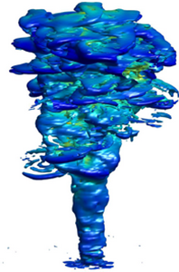
The schematic of the physical problem that is being investigated in this study is given in figure 1(a). At initial time  $t=0$, the ambient fluid of density
  $\rho _0$ and temperature
  $\theta _0$ is at rest. A circular region of the source at the bottom boundary with diameter
  $D(=400~\text {m})$ is heated with a constant surface heat flux (
 $H_o$). The heating causes a temperature difference (or density difference
  ${\rm \Delta} \rho$ with respect to the ambient density
  $\rho _0$) between the ambient fluid and the source region, which is represented by the reduced gravity
  $g^{\prime }=g ({{\rm \Delta} \rho }/{\rho _0})$. The domain is of size
  $10D \times 10D \times 17.5D$ along the two cross-stream (horizontal) and axial (vertical) directions, where
  $D$ is the diameter of the source located at the centre of the bottom boundary. The computational domain is discretized using a Cartesian grid with
  $100 \times 100 \times 700$ equidistantly spaced nodes in the cross-stream (horizontal) and axial (vertical) directions. The time step used in the simulations is chosen to be
  $1/6$ s in order to limit the Courant–Friedrichs–Lewy number to 0.2. Periodic boundary conditions were imposed on the side boundaries, while a constant pressure boundary condition was imposed on the top. At the centre of the bottom boundary, where the source is located, a constant surface heat flux is specified while the remaining bottom boundary has zero heat flux across. Table 1 summarizes the initial conditions considered for the simulation. A 5 % perturbation is imposed on the temperature field close to the source location by the cell perturbation method (Buckingham et al. Reference Buckingham, Koloszar, Bartosiewicz and Winckelmans2017). By imposing the perturbations on the temperature field, the turbulence build-up is supported by local buoyancy variations rather than the velocity field, as has been the case in many other studies (Schlüter, Pitsch & Moin Reference Schlüter, Pitsch and Moin2004; Wu Reference Wu2017).

Figure 1. Buoyant plume schematics in the study. (a) Instantaneous plume interface and leading edge location defined based on the reduced gravity threshold criterion,  $z_f$ and
  $z_c$ shown in panel (a) represent the instantaneous front height and axial location of maximum centreline velocity. (b) Time-averaged plume interface showing the neck region close to the source.
Table 1. Initial conditions and dimensionless numbers for cases simulated:  $H_o$ is the heat flux supplied at the source;
  ${\rm \Delta} \theta _{0}$ is the initial temperature difference between the source and ambience;
  $g^{\prime }_0$ is the initial reduced gravity at the source;
  $B_o$ is the rate of buoyancy addition at the source;
  $A_1$,
  $A_2$ are the Gaussian similarity constants for mean velocity and temperature radial profiles;
  $b_w$ and
  $b_{g^{\prime }}$ are the velocity- and buoyancy-half-widths of the plume scaled by the diameter
  $D$;
$D$;  $\overline {w_c}_{max}$ is the time-averaged maximum velocity along the centreline;
  $\tilde {z}$ and
  $\tilde {l}$ are the scaled axial location and plume half-width at the maximum velocity position (scaled by
  $D$).
$D$).

The simulations have been performed for five different cases with source  $g^{\prime }$ of 0.082, 0.145, 0.185, 0.237 and 0.272, respectively. Details of the simulations are given in table 1. The source heat flux is maintained at a constant value of
  $H_o$ which corresponds to 0.5, 1.0, 1.5, 2.0 and 2.5 km s
 $^{-1}$, respectively, for cases 1–5, which resulted in a
  ${\rm \Delta} \theta _0=\theta _0-\theta _{a}\approx 2, 4.5, 5, 7.3$ and 8.4 K (
 $\theta _{a}$ is the ambient temperature inside the domain). The simulation time is made dimensionless using a time scale,
  $t_0=D/w_b$, where
  $w_b$ is the buoyant velocity estimated as
  $\sqrt {g^{\prime }_{0} D}$. All the statistics reported in this study are time averaged starting from the time of formation of a well-defined head (discussed later) until
  $t/t_0=50$. The schematic of instantaneous state of the plume is shown in figure 1(a). The time-averaged mean state of the plume is shown in figure 1(b). The plume interface is defined based on the
  $g^{\prime }$ criterion, i.e. a 1 % threshold value of the source
  $g^{\prime }$.
The plume Reynolds number for the cases studied is defined based on the maximum mean velocity at the centreline ( $\overline {w_c}_{max}\!$) and plume half-width (
 $\tilde {l}$) at the axial location (
 $\tilde {z}$) of maximum velocity,
 \begin{equation} Re_{w_c}=\frac{\overline{w_c}_{max} \tilde{l}D}{\nu}, \end{equation}
where  $\nu$ is the viscosity of air estimated based on the temperature at
  $\tilde {z}$. Similarly, the Froude number is defined as a ratio of
  $\overline {w_c}_{max}$ and buoyancy velocity,
  $w_b$,
 \begin{equation} Fr_{w_c}=\frac{\overline{w_c}_{max}}{w_b}. \end{equation}
The turbulence Reynolds number based on  $\overline {w_c}_{max}$,
  $\tilde {l}$ and subgrid turbulent kinetic energy (
 $\overline {e}$) is estimated as
 \begin{equation} Re_{t}=\frac{\overline{w_c}_{max} \tilde{l}D}{\sqrt{\overline{e}}}, \end{equation}
where  $Re_{t}$ for the cases studied varied from 7364 to 9600 for cases 1–5, respectively.
3. Results
The coordinate system used is as follows: the components of the velocity are the axial velocity ( $w$) along the axial direction (
 $z$); the horizontal velocity components are (
 $u$) and (
 $v$). The leading edge of the plume is defined as the front, and it is mathematically represented as the leading point on the centreline (
 $r/D=0$) in the axial direction, where the plume buoyancy (
 $g^{\prime }$) is
  $1\,\%$ of source buoyancy (
 $g^{\prime }_{0}$). Similarly, the plume interface is defined using the
  $g^{\prime }$ threshold criterion. The time-averaged plume interface is used to obtain the plume half-width of the buoyancy profile (
 $b_{g^{\prime }}$) and of the velocity profile (
 $b_w$) at each height. We will refer to these as buoyancy half-width and velocity half-width, respectively. The plume front is defined as the leading location on the centreline of the plume at a given time. The plume velocity (
 $w_f$) is defined as the velocity of the plume front.
3.1. Plume characteristics
The plume characteristics are discussed first. The analysis of the plume characteristics has been performed for cases 1–5. Figure 2(a–c) are the plume characteristics for case 2. All the five cases are shown in figure 2(d). Figure 2(a) shows the velocity and buoyancy half-widths of plumes for case 2. Also shown in the figure are the experimental measurements from Ezzamel, Salizzoni & Hunt (Reference Ezzamel, Salizzoni and Hunt2015). It should be noted that the experimental results are for low buoyancy forcings (with  $g^{\prime }$ of 0.025) compared with the present study. Near the source, the plume radius decreases, reaches a minimum value and then increases, clearly showing a change of curvature from a converging to diverging trend, which is referred to as a neck region and this is a characteristic feature of area-release plumes. We estimated the plume Richardson number
  $\Gamma$ (Morton Reference Morton1959; Hunt & Kaye Reference Hunt and Kaye2001) using the local volume
  $(Q(z)=2{\rm \pi} \int _{0}^{\infty } w(r,z) r\, {\textrm {d}}r)$, momentum
  $(M(z)=2{\rm \pi} \int _{0}^{\infty } w^{2}(r,z) r\, {\textrm {d}}r)$ and buoyancy fluxes
  $(B(z)=2{\rm \pi} \int _{0}^{\infty } w(r,z) g^{\prime }(r,z) r\, {\textrm {d}}r)$,
 \begin{equation} \Gamma(z) = \frac{5}{2^{7/2}{\rm \pi}^{1/2}\alpha_{ref}}\frac{Q(z)^{2} B(z)}{M(z)^{5/2}}, \end{equation}
where  $\alpha _{ref}$ represents the reference entrainment coefficient which is considered to be 0.1 (Morton Reference Morton1959).

Figure 2. (a) Variation of velocity- and buoyancy-half-widths of the plume with height for case 2. (b) Variation of plume Richardson number with height for case 2. (c) For case 2, time–height variation of buoyancy half-width. The ( $+$) symbols represent the plume front and the solid line is 3/4 power law with respect to the time, and the dashed line represents the mean neck location along the plume axis. (d) For all the five cases, axial profile of
  $\lambda = {b_{g^{\prime }}/b_w}$. The filled circles and hollow triangles in panel (a) represent the half-widths based on buoyancy and velocity from experimental data of Ezzamel et al. (Reference Ezzamel, Salizzoni and Hunt2015). Filled circles and squares in panel (b) represent the experimental data of Ezzamel et al. (Reference Ezzamel, Salizzoni and Hunt2015) and LES data from Devenish et al. (Reference Devenish, Rooney and Thomson2010).
Figure 2(c) shows the variation of the plume height and buoyancy half-width in the  $t-z$ plane (
 $t$ is the time and
  $z$ is the vertical coordinate). Right after the release time, the plume radius decreases (converging trend) and reaches a minimum width beyond which it grows. A dotted line is shown to indicate this neck region. The rate at which the plume height increases is proportional to
  $t^{3/4}$, as depicted by the solid line which represents the
  $3/4$ power law. The presence of the neck has been confirmed by experiments, including those by Epstein & Burelbach (Reference Epstein and Burelbach2001) and Kaye & Hunt (Reference Kaye and Hunt2009). Finally, the ratio of the buoyancy half-width to the velocity half-width (
 $\lambda = b_{g^{\prime }}/b_w$), a measure of the ratio of the spread of the buoyancy to the spread of velocity profiles, is shown in figure 2(d). All the five cases have been reported here. The average value of
  $\lambda$ above the necking region is found to be around 1.15 for all the cases. For a plume-like behaviour, this value has been reported to be 1.19 (Papanicolau & List Reference Papanicolau and List1988), 1.2 (Panchapakesan & Lumley Reference Panchapakesan and Lumley1993) and 1.0 (Wang & Law Reference Wang and Law2002). They also noticed a general trend of a decreasing
  $\lambda$ with an increasing Richardson number. The Prandtl number (
 $\langle {\textit {Pr}_T}\rangle$), estimated as
  $\langle {\textit {Pr}_T}\rangle ={\lambda }^{-2}$, has a value of
  $0.75\pm 0.04$. Kaminski, Tait & Carazzo (Reference Kaminski, Tait and Carazzo2005) reported a tendency of
  $Pr$ to decrease with height. A similar trend is observed in our case. The variation of
  $\Gamma$ with height for case 2 is shown in figure 2(b). As expected,
  $\Gamma$ tends to infinity at the source as this is a pure buoyancy source with no momentum. Here
  $\Gamma$ reduces quickly until
  $\sim 2D$ and thereafter it asymptotes to a value
  $\Gamma =1$ after
  $\sim 5D$, as predicted by the theory for plumes where source
  $\Gamma \gg 1$ (Hunt & Kaye Reference Hunt and Kaye2005). The axial profiles of
  $\Gamma$ compare well both with the experimental data of Ezzamel et al. (Reference Ezzamel, Salizzoni and Hunt2015) and the LES data of Devenish et al. (Reference Devenish, Rooney and Thomson2010).
To quantify the plume's frontal motion, we identify the leading edge, or the plume front ( $z_f$) and plot versus time for cases 1–5 in figure 3(a). The front is defined as the farthest point along the centreline of the plume, where the plume interface is based on the threshold criterion of
  $g^{\prime }$. In this plot, the time is normalized by the time scale (
 $t_o$) based on the source diameter and buoyancy velocity (
 $w_b=\sqrt {g^{\prime }_0 D}$). Scaled in this manner, after the formation of the well-defined head (this will be discussed later on), the front (
 $z_f$) advances at a rate of
  $t^{3/4}$. The frontal velocity (
 $w_f$) which depends only on the buoyancy flux (
 $B_o$) and
  $z_f$ can be expressed as follows:
  $w_f= \xi _f B_o^{1/3} z_f^{-1/3}$, where
  $\xi _f$ is the non-dimensional front velocity. Using the definition
  $w_f={\textrm {d}}z_f/{\textrm {d}}t$,
  $\xi _f$ can be mathematically represented as
 \begin{equation} \xi_f= \frac{z_f^{4/3}}{B_o^{1/3}(t+t_s)(4/3)}, \end{equation}
where  $t_s$ is the time take for the head to form. The variation of non-dimensional velocity
  $\xi _f$ is plotted in figure 3(b). The plumes travel with a front velocity given as
  $w_f \approx 2.0 B_o^{1/3} z^{-1/3}$. The asymptotic value of non-dimensional front velocity scale (
 $\xi _f$) reached for all the cases is in the range of 1.89–2.05, matching closely with the 1.99 observed in Bhamidipati & Woods (Reference Bhamidipati and Woods2017). The Froude number for the cases has been calculated using the maximum centreline mean velocity and the buoyancy velocity. They are found to be 1.091, 1.089, 1.110, 1.141 and 1.149 for cases 1–5, respectively.

Figure 3. Variation in time of (a) non-dimensional plume front location ( $z_f/D$), (b) non-dimensional front velocity (
 $\xi _f$) and (c) non-dimensional centreline maximum velocity (
 $\xi _{wc}$) with respect to the non-dimensional time (
 $t/t_0$). The slope of the decay estimated from the mean centreline velocity is
  $-0.39 \pm 0.024$ for
  $2 \leq z/D \leq 12$.
Similar to the argument we made for the front velocity, the maximum centreline mean velocity can be scaled in terms of  $B_o$ and the height (
 $z_c$) where the maximum velocity occurs, and can be expressed as
  $w_c= \xi _{wc} B_o^{1/3} z_c^{-1/3}$, where
  $\xi _{wc}$ is the non-dimensional velocity, and the integration will lead to an expression for
  $\xi _{wc}= {z_c^{4/3}}/{B_o^{1/3}(t+t_s)(4/3)}$. The variation of
  $\xi _{wc}$ is plotted in figure 3(c). The non-dimensional maximum centreline mean velocity has a mean value of 2.83 with a standard deviation of 0.2. It should be noted the scatter is observed in
  $\xi _{wc}$ as this is the variation of the instantaneous axial location of the maximum centreline velocity, whereas the mean component is used to determine the decay rate. It can be established that for a pure plume in a neutral environment, the ratio of the non-dimensional front velocity to maximum centreline mean velocity is 0.7 for all the five cases. It is clear that as the plume develops, the fluid in the trailing region of the flow (as the maximum centreline mean velocity occur close to the source, which is in the range of
  $1.5D\text {--}1.8D$ for the five cases) travels faster than the frontal region and thus trailing source fluid is continuously fed into the frontal region or the head of the plume causing unsteady effects. This is a characteristic feature of the starting plumes that results in the dilution and mixing of the head region of the plume that is constantly fed by the trailing edge of the plume. Similar dynamics of source fluid feeding into the active head region from the passive trailing region were also observed in buoyancy driven lock-exchange density currents (Bhaganagar Reference Bhaganagar2017). The maximum centreline buoyancy and maximum centreline velocity are the characteristic buoyancy and velocity scales, respectively. The results have been shown for case 2, and similar values for the non-dimensional front velocity and maximum centreline velocity have been obtained for all the five cases. Turner (Reference Turner1962) found out from his experiments that the front of a starting plume travels with
  $\approx 61\,\%$ of the plume velocity at respective heights once it reaches steady-state. In the present study, the plume velocity within the similarity regime is calculated and the ratio came out to be
  $0.64\pm 0.03$, matching closely with the results of Turner (Reference Turner1962) and Bhamidipati & Woods (Reference Bhamidipati and Woods2017).
3.2. Mean flow characteristics
The time-averaged mean flow characteristics at the centreline ( $r=0$) are discussed first. The results for case 2 are shown. Figure 4(a) shows the mean velocity at the centreline normalized by the maximum value (
 $\overline {w_c}$), plotted against the axial distance from the source
  $z$ scaled by the source diameter,
  $D$. Initially, the centreline mean velocity accelerates up to
  $z=1.6D$, reaches a maximum value
  $\overline {w_{c}}_{max}$, and starts to decay at a rate of
  $-{1}/{3}$ power law with height. Also plotted in this figure are the experimental measurements obtained by Pham, Plourde & Doan (Reference Pham, Plourde and Doan2005), LES results of Pham et al. (Reference Pham, Plourde and Doan2007) and from the direct numerical simulation (DNS) by Plourde et al. (Reference Plourde, Pham, Doan and Balachandar2008). It should be noted that these LES, DNS and experiments have been conducted at much smaller Reynolds number and
  $B_o$. The current simulations show a good agreement with previous results. Similar trends have been observed for the other cases; however, the location where is regime shifts to the power-law shows a very weak trend with
  $B_o$. For cases 1–5, the location of maximum velocity occurs at
  $1.62D, 1.63D, 1.63D, 1.75D$ and
  $1.75D$, respectively.

Figure 4. For case 2, axial profiles of (a) normalized centreline mean velocity and (b) normalized centreline mean temperature difference.
Similar analysis has been performed on the mean temperature difference at the centreline ( $\overline {{\rm \Delta} \theta _c}$ in figure 4(b)), which is the difference between the temperature in the plume with respect to the ambient temperature. Initially, the centreline mean temperature difference decreases slowly from the source conditions; there is a regime shift and it exhibits a faster decay at a rate of
  $-{5}/{3}$ consistent with theory. An analytical solution for the asymmetric vertical turbulent plume was developed by Batchelor (Reference Batchelor1954) who proposed a similarity solution for the mean axial velocity and mean buoyancy acceleration (measure of the temperature difference between the plume and the ambience) as follows:
  $w= B_o^{1/3}z^{-1/3}f_w(r/z)$ and
  $g^{\prime }=B_o^{2/3}z^{-5/3}f_b(r/z)$, respectively, where
  $B_o$ is the rate at which buoyancy is added at the source,
  $z$ is the height,
  $r$ is the radial distance,
  $g^{\prime }$ is the buoyancy acceleration,
  $f_w$ and
  $f_b$ are the similarity functions. The LES conducted in this study show a good agreement with the theoretical prediction of
  $-1/3$ and
  $-5/3$ power law for the centreline mean temperature difference and centreline mean velocity of the axisymmetric plume, respectively.
The radial profiles of the mean flow are discussed next. The radial profiles of the scaled mean axial velocity and the scaled mean temperature difference are plotted at different heights for case 2 in figure 5(a,b), respectively. The radial profiles of mean axial velocity and mean temperature exhibit self-preservation characteristics as they collapse to a single curve. The least square Gaussian fit of the mean axial velocity is obtained as  $f_w(r/z) = \overline {w_c}\exp [-91.75 (r/z)^{2}]$ for case 2. The coefficient varies with
  $B_o$, and the values for cases 1–5 are
  $-$82.07,
  $-$91.75,
  $-$91.39,
  $-$88.19,
  $-$94.88, respectively. For the mean temperature, this fit is obtained as
  $f_b(r/z)=\overline {\theta _c}\exp [-78.337 (r/z)^{2}]$. The coefficients of the Gaussian fit are close to the ones found by Papanicolau & List (Reference Papanicolau and List1988) and they depend on
  $B_o$ as seen in table 1. The coefficients for cases 1–5 are
  $-$75.02,
  $-$78.34,
  $-$81.28,
  $-$82.86 and
  $-$85.39, respectively. The maximum mean velocity occurs at the centreline (
 $r=0$). The buoyancy profiles are wider compared with the velocity profiles, and this is consistent with measurements of plume half-width (
 $b_w$) obtained from the mean velocity profile and plume half-width (
 $b_{g^{\prime }}$) obtained from the mean buoyancy profile (see figure 2a), thus indicating that buoyancy mixing is more dominant than shear mixing in plumes. We will discuss the turbulence characteristics, in detail, in the next section.

Figure 5. Similarity profiles of (a) mean axial velocity and (b) mean temperature normalized with their respective centreline values for case 2 plotted at different heights above the source. The least squares Gaussian fit is shown by a solid line. Same similarity observed for all the other cases as well.
The axial evolution of the plume is discussed next. Figure 6(a) shows the axial profiles of the mean velocity at different radial locations for case 2. At the centreline  $r= 0$,
  $\overline {w}$ increases slowly from zero to a maximum velocity which occurs at
  $z=1.62D$ above the source. Beyond this height, it decays. As seen from figure 4(a), the decay has been calculated to be a power law of
  $-{1}/{3}$ with height. At radial distances away from the centreline, the trend of the mean flow is different. For example, at
  $r=0.2D$, the mean flow accelerates up to a height of
  $z=4D$ and it stays nearly constant above this height. A similar trend is evident at radial distances towards the edge of the plume, the mean flow initially accelerates, and then reaches a quasi-steady value. Figure 6(b) shows the profiles of the mean buoyancy at different radial locations.

Figure 6. Axial profiles of (a) mean axial velocity and (b) mean buoyancy at radial distances as specified in the legend for case 2.
In conclusion, the mean characteristics of the starting plume reveal that mean flow velocity scales with  $B_o$ and
  $z$, with the front moving 0.7 times slower than the trailing regime of the plume. The average buoyancy half-width is
  $10\,\%$ wider than the velocity half-width. In the neck region, the mean flow accelerated and reached a maximum velocity, beyond which a regime shift occurs. Mean profiles exhibit self-similarity only above the neck region.
3.3. Turbulence characteristics
We begin the analysis of turbulence by examining turbulence intensity, which is the relative measure of the r.m.s. of velocity and buoyancy fluctuations. All the five cases are analysed here. Figure 7(a) shows the scaled axial profiles of the r.m.s. of buoyancy fluctuations at the centreline, while figure 7(b,c) show the scaled axial profiles of the r.m.s of the axial velocity and horizontal velocity fluctuations at the centreline, respectively. In the near-source region the buoyancy and velocity fluctuations develop and reach a quasi-equilibrium state away from the source. The  $\theta _{rms}$ varies between 0.48–0.53 fraction of the mean temperature for different cases. For a fully developed plume, this value has been reported to be in the range of 0.36–0.46 (George, Alpert & Tamanini Reference George, Alpert and Tamanini1977; Ezzamel et al. Reference Ezzamel, Salizzoni and Hunt2015; Van Reeuwijk et al. Reference Van Reeuwijk, Salizzoni, Hunt and Craske2016) as shown in table 2. The fractional values of
  $w_{rms}$ and
  $u_{rms}$ with respect to the mean centreline velocity vary from 0.31–0.35 and 0.21–0.24, respectively. These values have been reported to be in the range of 0.19–0.30 and 0.15–0.20, respectively (see table 2). Figure 7(d) shows the correlation between axial velocity fluctuation and buoyancy fluctuation,
  $\overline {{w^{\prime }\theta ^{\prime }}}$, which achieves a maximum value at a height of
  $z=2D\text {--}4D$, and corresponds to the 0.11–0.13 fraction of the correlation of mean axial velocity and buoyancy. As reported in previous experiments for steady-state plumes, the relative buoyancy fluctuations in starting plumes are stronger compared with the velocity fluctuations. This is reasonable to expect, as plumes are buoyancy driven in nature.

Figure 7. Axial variation of (a) r.m.s. of temperature fluctuations scaled by centreline mean temperature, (b) r.m.s. of axial velocity fluctuations scaled by centreline mean axial velocity, (c) r.m.s. of horizontal velocity fluctuations scaled by centreline mean axial velocity, (d) r.m.s. of turbulent buoyancy flux normalized with correlation of centreline mean velocity and centreline mean temperature.
Table 2. Comparison of the r.m.s. of turbulence fluctuations against the existing literature. First five rows correspond to present study cases 1–5.

The radially averaged profiles of the r.m.s. of the axial and radial velocity fluctuations and buoyancy fluctuations for all the five cases are shown in figure 8. The peak r.m.s of velocity and buoyancy fluctuations increases with increasing source buoyancy  $B_o$. The peak value of axial velocity fluctuations occurs at a height of
  $z=4D$ above the source, whereas the radial velocity fluctuations reach a maximum at
  $5D$. At the centreline, due to the presence of the source, the buoyancy fluctuations are highest at the surface. They initially decay up to height to
  $z=1D$, beyond which they reach a quasi-equilibrium value in the region
  $z=1D\text {--}4D$, followed by monotonic decay. The radially averaged buoyancy profile exhibits a similar trend. For higher source strength,
  $B_o$, turbulence velocity fluctuations persist even at heights corresponding to
  $z=15D$; on the other hand, the buoyancy fluctuations decay much faster as they vanish around
  $z=10D$ above the source for all the cases. The decay of the radial velocity fluctuations with height is much slower compared with that of the axial velocity fluctuations. The peak turbulence intensity occurs higher above the source compared with the peak centreline mean velocity, which occurs around
  $z=1.2D$. The location of the peak r.m.s. velocity fluctuations coincide with the beginning of the instabilities leading to mixing and entrainment. This will be discussed further in the next section. The axial profiles of TKE are shown in figure 8(d). Turbulence kinetic energy reaches a maximum value at
  $4D$, and the higher the
  $B_o$, the higher is the TKE magnitude. Turbulence kinetic energy decays with height, but is still persistent at
  $z=15D$.

Figure 8. Axial variation of radially averaged profiles of the r.m.s. of the (a) temperature fluctuations, (b) axial velocity fluctuations, (c) horizontal velocity fluctuations, (d) turbulent kinetic energy for all the cases.
Turbulence kinetic energy profiles at different radial locations for case 2 are plotted in figure 9(a). At the centreline ( $r/D=0$), the maximum TKE occurs at
  $z=4D$ from the source. Off the centreline, the location of the maximum TKE moves away from the source with increasing radial distance from the centreline. To estimate at what radial distances the maximum TKE occurs at different height above the ground, figure 9(b) shows the radial location corresponding to the maximum TKE at each height. In the near-source region, the maximum TKE occurs at the centreline. However, at spatial locations beyond the height of
  $5D$, the location of the maximum TKE moves radially away towards the plume interface. The maximum TKE at each height is also plotted here. Far away from the source at
  $z=15D$, the TKE is still strong and it has a magnitude which is
  $33\,\%$ of the maximum TKE. Figure 9(c) shows the TKE scaled by maximum TKE in the plume (this occurs at the centreline) plotted against radial distance scaled by the height. As all the profiles have been scaled by a common denominator, the relative strengths of the TKE at different elevations is apparent. Scaled in this manner, the TKE profiles show a similarity radially away from the centreline. Difference in TKE is evident up to
  $r= 0.1z$, and beyond which the profiles collapse in both near- and far-regions from the source.

Figure 9. For case 2, (a) axial profiles of TKE at various radial distances, (b) radial location of the maximum TKE (circle symbols) and the magnitude of the maximum TKE at each axial plane, (c) radial profiles of TKE normalized with the maximum value at different axial distances given in the legend below.
The scaled radial profiles of the r.m.s. of the velocity and buoyancy fluctuations for case 2 are plotted in figures 10(a) and 10(b), respectively. The mean flow has reached a similarity at these time scales, whereas the turbulence has not yet reached a state of self-similarity. There is a significant scatter present for the similarity profiles. The radial profiles of the shear driven and the buoyancy driven TKE production for case 2 are shown in figures 11(a) and 11(b), respectively. The TKE production is due to combination of shear production ( $P_s=-\overline {u^{\prime } w^{\prime }}[{\partial {\overline w}}/{\partial {r}}+{\partial {\overline u}}/{\partial {z}}]$) and buoyancy production (
 $P_b=-\overline {w^{\prime } \theta ^{\prime }}(g/\overline {\theta }$)) of turbulence. The Reynolds stresses (i.e.
  $\overline {w^{\prime } u^{\prime }}$) contribute to the shear production, and temperature velocity correlation (
 $\overline {\theta ^{\prime } w^{\prime }}$) contribute to the buoyancy production of TKE. As seen in figure 11(a), peak
  $P_s$ occurs at an off-axis location of
  $0.25D$ from the axis at
  $z=2D\text {--}4D$. At these heights, the peak
  $P_b$ also occurs at the same radial location. In the near-source region, both shear and buoyancy production are maximum at
  $r=0.25D$, whereas the maximum TKE occurs at the centreline, clearly indicating a radial transport of turbulence towards the axis. Away from the source, at heights
  $z=4.5D\text {--}6.5D$, the peak
  $P_s$ is off-axis at
  $r=0.4D$. This is mainly due to the fact that in the near-source region, the shear production is mainly dominant due to the shearing mechanism at the centreline. On the other hand, the peak
  $P_b$ is confined to
  $r=0.2D\text {--}0.4D$. The magnitude of the buoyancy production is higher compared with the shear production of turbulence, as expected. The driving force is due to buoyancy flux and only a portion of the buoyancy flux is converted to the momentum flux.

Figure 10. Radial profiles of the scaled (a) r.m.s. of the axial velocity fluctuations, (b) r.m.s. of the buoyancy fluctuations for case 2. The symbols correspond to the locations as given in figure 9(c).

Figure 11. Radial profiles of (a) TKE shear production ( $P_s$) and (b) TKE buoyant production (
 $P_b$) at various axial locations along the plume growth for case 2. The symbols correspond to the locations as given in figure 9(c).
In summary, the starting plumes from an area release are characterized by a converging–diverging neck that corresponds to a location of minimum radius and maximum velocity. The axial mean velocity develops a similarity solution of the form  $\overline {w_c}=B_o^{1/3} z^{-1/3} e^{A_1 (r/z)^{2}}$ and the axial buoyancy has a form
  $\overline {\theta _c}=B_o^{2/3}z^{-5/3} e^{ }{A_2 (r/z)^{2}}$, where
  $\overline {w_c}$ and
  $\overline {\theta _c}$ denote the mean centreline velocity and temperature, respectively, and
  $A_1$ and
  $A_2$ correspond to the Gaussian similarity coefficients for
  $\overline {w_c}$ and
  $\overline {\theta _c}$ given in table 1. It is estimated from
  $\lambda$ that the neck exists and extends to 5
 $D$. Turbulent kinetic energy is generated due to a combination of shear and buoyancy driven production mechanisms. Both the peak TKE production mechanisms,
  $P_s$ and
  $P_b$, occur in the neck region, off-axis from the centreline at heights of
  $z=3D$ and
  $z=2D$, respectively. The peak TKE production occurs off-axis but due to radial transport mechanisms the peak TKE occurs at the centreline. The maximum TKE occurs at a height
  $4D$ above the source and beyond which it starts to decay. The buoyancy fluctuations vanish by the height of
  $10D$ above the source. The velocity fluctuations reach a peak value at
  $4D$ above the source, and the higher the
  $B_o$, the higher their magnitude. They persist longer, and at a distance of
  $12D$ above the source, the magnitude is still significant. The near-source TKE is mainly due to buoyancy-generated turbulence, whereas the shear-generated turbulence contributes to TKE in the far-source region.
3.4. Flow structures, mixing and entrainment
In this section, we investigate the mixing processes as the plume expands into the atmosphere, entraining the ambience and spreading radially. We first discuss the flow structures. To understand the differences in the vortex structures between the cases, the following analysis is conducted for all the five cases. The evolution of the isosurfaces of instantaneous buoyancy ( $g'$) at two different times corresponding to
  $t=400$ and 1300 s after release is shown in figure 12 for all the five cases. After
  $t=200$ s, a central core is formed (this is not shown). The time taken for the central core to form is nearly the same for all the cases. As the plume accelerates vertically with increasing mean velocity at the centreline, the velocity difference between the ambience and the core results in the formation and eventual roll-up of the shear layer into primary vortical structures. These arise mainly due to the Kelvin–Helmholtz shear-driven instability. At
  $t=400$ s, a well-defined head is evident characterized by instabilities at the interface for cases 2–5. The head has still not formed for the case 1 (lowest forcing), and it forms at a later time. The higher the
  $B_o$, the faster is the formation of the head. This happens around
  $z= 2D$ for all the cases. As the plume travels beyond
  $z=2D$, the plume enters a decelerating regime where the centreline mean velocity starts to decay resulting in growth of instabilities, whereupon it becomes unstable and breaks down into smaller vortices. A characteristic feature for all the cases is the development of a well-defined neck region which is capped by the unstable head as seen from figure 12(b,d,f,h,j) at time
  $t=1300$ s. The vortical structures that form above the neck and that will be referred to as the head region of the plume, grows in size as the plume expands. The higher the
  $B_o$, the instabilities in the head region are more dominant that cause the ambient fluid to be entrained into the plume and resulting in increased mixing.

Figure 12. Isosurfaces of instantaneous buoyancy  $g^{\prime }$ for case 1 (a,b), case 2 (c,d), case 3 (e,f), case 4 (g,h) and case 5 (i,j) at
  $t= 400$ s (a,c,e,g,i) and
  $t = 1300$ s (b,d,f,h,j).
For the rest of the analysis of the flow structures, we present the analysis for one case and for consistency with the rest of the manuscript, we pick case 2. The buoyant fluid from the source rises vertically in a column with an upward-spiralling motion as depicted in figure 13. Figure 13(a) shows the  $\lambda _2$ vortex detection criterion (Jeong & Hussain Reference Jeong and Hussain1995) which is used to extract the dominant vortex features plotted at time
  $t=1740$ s after the initial source release. The conspicuous feature that is evident is the formation of a column of upward-spiralling vortices that is present to a height of
  $z=5D$ above the source. The primary vorticity is generated mainly due to buoyancy. Above the column vortex, horizontal vortex rings form that propagate upwards as the plume grows. The vorticity transport equations dictate that the buoyancy can only generate vorticity in the radial direction, which is the primary component of vorticity; and the tilting of the horizontal vorticity into the axial direction results in the secondary vorticity, thus forming the axial vorticity (Tennekes & Lumley Reference Tennekes and Lumley1972). The isosurfaces of vorticity at time
  $t=2100$ s are plotted for two different contour values to extract the features of the column vortex and the horizontal vortex rings in figures 13(b) and 13(c), respectively. The column vortex consists of positive vorticity (clockwise in nature) as it spirals upwards with increasing vorticity. Counter rotating vortices (negative vorticity) stretch in the horizontal plane and expand along the plume direction. Such similar counter-rotating vortices in the far-field aligned with the plume trajectory have been observed for a jet in a cross-flow (Fric & Roshko Reference Fric and Roshko1994). Wildland fires have exhibited characteristic horizontal vortex rings, forms that propagate upwards as the plume grows (Forthofer & Goodrick Reference Forthofer and Goodrick2011). Figure 14 shows the contours of the instantaneous buoyancy (
 $g^{\prime }$) as the plume evolves in time for case 2. At a time
  $t=300$ s after the release of the plume, a well-defined head emerges consisting of the heated fluid at source conditions. At
  $t=360$ s, instabilities appear near the front and mixing is initiated. At
  $t=600$ s, the frontal region of the plume expands with the head still maintaining its shape. At this time, instabilities are initiated at the centreline. As the time progresses to
  $t=780, 1500$ and
  $2400$ s, the plume expands with increasing dilution near the frontal region of the plume. Even at the later times, the mixing at the central core of the plume starts only beyond a distance of
  $z=2D$ from the source. The mixing and entrainment is a highly unsteady process. We will quantify the mixing using a first principles approach.

Figure 13. For case 2: (a)  $\lambda _2$ vortex detection criterion isosurface with
  $\lambda _2=-3e^{-5}$ at
  $t=1740$ s, (b) 0.05 isosurface of vorticity at
  $t=2100$ s, (c) 0.02 isosurface of vorticity at
  $t=2100$ s. The isosurfaces in (a–c) are coloured according to the instantaneous axial velocity, the colourbar is given in (a).

Figure 14. Time evolution of instantaneous buoyancy,  $g^{\prime }$, at the centreplane for case 2.
Figure 15(a,b) shows the contour plot of instantaneous radial vorticity and axial vorticity, respectively, as the plume evolves from the source. This is presented for case 2. In the initial stages at  $t=300, 360$ s with the formation of the head, buoyancy generated radial vorticity originates at the source and expands vertically as the plume moves forward. This is seen from figure 15(a), which depicts the radial vorticity contours. At later times, the vortex structures around the centreline expand to
  $z=5D$ at
  $t=780$ s, and beyond which, at later times, i.e.
  $t=1500, 2400$ s, the spatial instabilities break the vorticity resulting in the formation of small-scale structures above this height at later times. On the other hand, the axial vorticity that develops is the secondary vorticity from the vortex stretching and tilting processes. It is characterized by small-scale structures even at earlier times. At later times, due to instabilities at the front interface, the vortex breakdown results in the entire plume being dominated by small-scale structures. The unsteady mixing and dilution at the frontal region of the plume results in instabilities and leads to the breakdown of the vorticity to small-scale structures.

Figure 15. Instantaneous snapshots of (a) radial vorticity and (b) axial vorticity for case 2.
Figure 16 shows the instantaneous velocity vectors in the  $r\text {--}z$ plane at
  $t=1300$ s for case 2. Dominant features of the plume include a neck region with a primarily axial component of velocity, and strong instabilities at the plume interface that entrain the ambient fluid into the plume and result in significant mixing. Strong mixing is evident at the frontal region of the plume.

Figure 16. For case 2, cross-stream averaged velocity vectors and plume contour selected by  $g^{\prime }$ threshold at centreplane at
  $t=1300$ s. Here, A1 and A2 are plume cross-sections at
  $3.6D$ and
  $8.5D$, respectively.
The unsteady entrainment is the most prominent feature of starting buoyant plumes, and it is calculated using first principles as follows: the amount of fluid that entrains into the plume in a small time interval is the change in the volume of the plume during that time period. With increasing source buoyancy flux, the plume expands much faster as the cold ambient entrains more efficiently, mixing and diluting the plume. The instantaneous scaled entrainment  $E$, is the amount of the ambient fluid that enters the current, and it is calculated as the increase of the volume of fluid in the plume due to the radial expansion of the plume with respect to the previous state in time per unit volume of the initial fluid; it is defined as
 \begin{equation} E(t) = \frac{V (t_2)-V(t_1)}{A_{neck} u_f\, {\textrm{d}}t}. \end{equation}
Here,  $V(t_2)$ and
  $V(t_1)$ represent the volume of the fluid in the plume at instants
  $t=t_1$ and
  $t_2$, respectively. The radial expansion of the plume during the time interval
  ${\textrm {d}}t=t_2- t_1$ is given as the change of the volume (change of the area times the distance travelled by the plume during this time), where the distance travelled by the plume is
  $u_f \, {\textrm {d}}t$ and the area of the initial release is
  $A_{neck}$. A similar approach of using the volume-based measure to quantify the entrainment has been conducted successfully by Bhaganagar & Pillalamarri (Reference Bhaganagar and Pillalamarri2017).
Figure 17(a) shows the instantaneous scaled entrainment  $E$ versus time for all the cases. The entrainment begins after the formation of the head (which occurs around
  $z=2D$ from the source). It increases to a maximum value and it steadily drops and reaches an asymptotic value, which varies from 0.05–0.08 for cases 1–5. The maximum E is 0.15 for the case with the highest
  $B_o$. The time where the peak entrainment occurs correlates with the time when the mixing is initiated in the plume, and due to the entrainment of the cooler ambient fluid into the plume, it undergoes dilution with drastic reduction of the buoyancy. The higher the source buoyancy flux, the higher the entrainment and the longer it takes to reach a steady-state value. Figure 17(b) shows the entrainment parameter verses the local Reynolds number. There is a correlation (
 $R^{2}=0.62-0.69$) with the local Reynolds number. This is reasonable as the entrainment occurs in the unstable head region which moves with the front velocity and the local width of the plume. The local Reynolds number has been calculated based on the width of the plume in the head region and the front velocity.

Figure 17. (a) Variation of the scaled entrainment ( $E$). The dashed lines represent the respective average scaled entrainment values over the period plotted. (b) Correlation of
  $E$ with local Reynolds number.
Significant variability in the entrainment coefficient has been reported in the literature. The classical plume theory estimates the entrainment coefficient as 0.15, whereas George et al. (Reference George, Alpert and Tamanini1977) estimated the entrainment coefficient in the far-field of the plume as 0.108 in the region where the mean velocity profiles were Gaussian. For Gaussian profiles, the entrainment coefficient has been reported in the range of 0.07–0.11 for pure buoyancy-dominated plumes (Carazzo, Kaminski & Tait Reference Carazzo, Kaminski and Tait2006). Papanicolau & List (Reference Papanicolau and List1988) calculated the entrainment coefficient to be 0.0875 for pure plumes.
4. Conclusions
Geophysical turbulent buoyant plumes that occur in the atmosphere have high Reynolds numbers, they expand vertically (several kilometres) and spread radially while entraining the ambient fluid, resulting in substantial mixing. Our understanding of the flow dynamics of starting turbulent buoyant plumes is still very limited. There is no consensus on the centreline mean velocity and buoyancy profiles nor the turbulence measurements such as ratio of the turbulence to the mean flow. Characteristic features of starting plumes from an area release have been reported in various studies as consisting of a converging–diverging region (neck), which is capped by a well-defined head region; however, the flow dynamics in these regions has not been well understood. Significant knowledge gaps exist in our understanding of the flow physics in the near-source region (0–15 $D$) of the plume. To address these issues, a fundamental study has been conducted to understand the mean and turbulence characteristics and the unsteady dynamics of large-scale structures, and their role in mixing processes of starting turbulent plumes initiated from a heated area-release source into the neutral atmosphere. Large eddy simulation has been conducted in a domain of size
  $7\ \text {km}$ in vertical and
  $4\ \text {km} \times 4\ \text {km}$ in horizon. Simulations have been performed for five different cases with source
  $g^{\prime }$ of 0.082, 0.145, 0.185, 0.237, 0.272, respectively. The source heat flux is maintained at a constant value ranging from 0.5–2.5 km s
 $^{-1}$. We define the plume Reynolds number based on maximum centreline velocity and the plume half-width at this height. With increasing
  $B_o$, the plume Reynolds number
  $Re$ increases from
  $6 \times 10^{7}\hbox{--}10^{8}$; however,
  $Fr$ does not increase monotonically with increasing
  $B_o$, and it varies from 1.091–1.149 for the five cases.
Buoyancy plumes released from an area source are characterized by a neck region resembling a column which extends to a height of  $5D$ and this region has a characteristic converging–diverging trend where the plume width decreases from the source radius and reaches a minimum, and beyond which the plume expands. The region above this columnar neck is the dynamically active head region where there is an active mixing, entrainment and dilution of the plume. The average value of the plume width of the temperature profile compared with that of the velocity profile above the neck region of the plume has been obtained as 1.15, which is consistent with plume-like behaviours as reported by previous experiments where the buoyancy profiles are wider than the velocity profiles at a given height.
The mean flow developed from the buoyancy forcings accelerates from rest to a maximum value and it starts to decay in height at a rate of a  $-1/3$ power law. The maximum velocity occurs in the neck region (varying in the range of
  $z= 1.62D\text {--}1.75D$ for the five cases). During the accelerating period, the mean buoyancy is nearly a constant and as the flow starts to decelerates, it also starts to decay, but at a rate of
  $-5/3$. The radial profiles of the mean temperature and buoyancy reaches a self-similarity behaviour with a Gaussian distribution from a height of
  $z=2D$ for all the cases. The mean flow is not self-similar in the neck region. The front velocity and the maximum centreline velocity scales with
  $B_o$ and
  $z$, and can be expressed as
  $w_f= \xi _f B_o^{1/3} z_f^{-1/3}$ as
  $w_c= \xi _{wc} B_o^{1/3} z_f^{-1/3}$, respectively. For all the cases, we obtained that the front moves with a non-dimensional velocity (
 $\xi _f$) of
  $\sim$2.0 and the non-dimensional maximum centrelinevelocity (
 $\xi _{wc}$) is
  $\sim$3.0. The consequence of this is that as the plume advances the fluid from the neck region overrides the front velocity and thus feeds into the head region of the front. It has important implications, resulting in the unsteady mixing and entrainment.
Initially, turbulence is mainly generated from the buoyancy production mechanisms ( $P_b$). The higher the
  $B_o$, the higher the initial production of TKE. In the near-source region,
  $2D\text {--}4D$, both
  $P_s$ and
  $P_b$ contribute to TKE, and with peak production at a radial location of
  $r=0.2D$. As the plume grows axially, the location of peak TKE production shifts radially outwards. Due to the radial transport of TKE towards the centreline, the maximum TKE is concentrated at
  $r/D=0$. Overall,
  $P_b$ is higher than
  $P_s$. The r.m.s of axial velocity and radial velocity fluctuations build from zero near the wall to quasi-equilibrium value at nearly
  $5D$, with values ranging from
  $w_{rms}$ of 0.31–0.35,
  $u_{rms}$ of 0.21–0.24 and
  $\theta _{rms}$ of 0.48–0.53, respectively. Buoyancy fluctuations are much dominant compared with the velocity fluctuations. It is interesting to note that the neck region of the plume plays an important role in the production of TKE, whereas the peak turbulence is mainly concentrated in the head region of the plume, which is dynamically active.
The entrainment and mixing is a highly unsteady process. Key physical structures that have been observed are the upward spiralling vortex with clockwise vorticity that forms the central core of the plume, and vortex rings that stretch in the horizontal plane which expand along the plume direction. During the initial accelerating stage, a well-defined head is formed that is characterized by a spiralling vortex with ring formation with the dominant radial component of vorticity generated by buoyancy. The primary mechanism for the formation of the head is shear-driven instability. As the plume expands over time, the spiralling central core strengthens that leads the instabilities to break down the structures to small scales in the head region of the plume. The spiralling central core expands to around  $5D$, thus forming a neck region and which is capped by the unstable head. This region is characterized by maximum TKE that occurs at the centreline. The fluid in the neck region (maximum centreline velocity occurs between
  $1.5D\text {--}1.7D$ for all the cases), travels faster than the front, thus constantly feeding into the head. Unsteady entrainment (
 $E$) has been quantified using first principles, and this revealed that, initially the entrainment is negligible until the formation of secondary instabilities leading to the breakdown of the structures. Here,
  $E$ correlated with the local Reynolds number based on the width of the head (dynamic portion of the plume) and front velocity.
Ultimately, this study is offered as a contribution to improve the understanding of starting plumes released from area source, where there is a scarcity of both experimental and numerical data. A framework has been developed to characterize starting plumes released in atmospheric conditions. The study has direct relevance to important applications for natural disasters, such as wildland-based fires, where the improved understanding of flow characteristics and unsteady entrainment are important for predicting the mixed state of the plume. The present study assumes the ambient air is in a neutral stability state, and future studies will be able to extend the knowledge gained from this study to isolate the effects of atmospheric stability on plume fluid dynamics. The presence of a spiralling column vortex around the central core and the vortex rings that cause the plume to spread as it entrains the surrounding cooler air and mixing rigorously are characteristic features of geophysical plumes. In future, the present study will be extended to include the effect of atmospheric stability on the unsteady entrainment processes, and the modification of the vorticity generation processes and vortex structures will provide key insights to the contribution of the atmospheric convective rolls on modifying the mixing processes.
Declaration of interests
The authors report no conflict of interest.


