


1. Introduction and background
Morphological characterization of high-Reynolds-number turbulent boundary layer flows over surfaces that exhibit geometric complexity is central to a number of practical flow scenarios (Raupach, Antonia & Rajagopalan Reference Raupach, Antonia and Rajagopalan1991; Jimenez Reference Jimenez2004; Castro Reference Castro2007). In particular, the momentum exchange between such flows and the bounding surface is critical to the performance of vapour power systems (Bons et al. Reference Bons, Taylor, McClain and Rivir2001) and naval architecture surfaces on which growth of biological mass has occurred (Schultz Reference Schultz2007). Some environmental flow problems of recent interest include erosion, transport and deposition of sediment by turbulent flows over subaqueous or aeolian bedforms (Best Reference Best2005; Livingstone, Wiggs & Weaver Reference Livingstone, Wiggs and Weaver2006; Palmer et al. Reference Palmer, Mejia-Alvarez, Best and Christensen2012), and surface fluxes of momentum and scalars (temperature, humidity) associated with atmospheric boundary layer flows over complex natural landscapes (Bou-Zeid, Meneveau & Parlange Reference Bou-Zeid, Meneveau and Parlange2005; Anderson Reference Anderson2013).
Early studies of roughness effects were dedicated to assessing head losses in flows through pipes of varying roughness (Nikuradse Reference Nikuradse1933; Colebrook & White Reference Colebrook and White1937). Schlichting (Reference Schlichting1937) investigated the role of varying roughness element topology and spatial distributions of elements. This work remains an open topic of enquiry. Recent efforts have focused on developing functional relations between the equivalent sand-grain roughness length,
 $k_{s}$
– used to parametrize the roughness function,
$k_{s}$
– used to parametrize the roughness function,
 ${\rm\Delta}U$
(momentum deficit due to the presence of roughness) – and statistical attributes of the roughness. Statistical attributes including roughness height, root-mean-square (r.m.s.) roughness and roughness skewness are commonly used in such parametrizations (Schultz & Flack Reference Schultz and Flack2009; Flack & Schultz Reference Flack and Schultz2010; Mejia-Alvarez & Christensen Reference Mejia-Alvarez and Christensen2010). Turbulence within the roughness sublayer is characterized by coherent structures with macroscale of the order of individual roughness elements (Castro Reference Castro2007); in the inertial sublayer above this, however, for
${\rm\Delta}U$
(momentum deficit due to the presence of roughness) – and statistical attributes of the roughness. Statistical attributes including roughness height, root-mean-square (r.m.s.) roughness and roughness skewness are commonly used in such parametrizations (Schultz & Flack Reference Schultz and Flack2009; Flack & Schultz Reference Flack and Schultz2010; Mejia-Alvarez & Christensen Reference Mejia-Alvarez and Christensen2010). Turbulence within the roughness sublayer is characterized by coherent structures with macroscale of the order of individual roughness elements (Castro Reference Castro2007); in the inertial sublayer above this, however, for
 ${\it\delta}/k\gtrsim 40$
(where
${\it\delta}/k\gtrsim 40$
(where
 ${\it\delta}$
is the boundary layer thickness), Townsend’s hypothesis states that flow statistics are independent of details of the roughness sublayer for adequately high Reynolds number (Townsend Reference Townsend1976; Raupach et al.
Reference Raupach, Antonia and Rajagopalan1991; Jimenez Reference Jimenez2004).
${\it\delta}$
is the boundary layer thickness), Townsend’s hypothesis states that flow statistics are independent of details of the roughness sublayer for adequately high Reynolds number (Townsend Reference Townsend1976; Raupach et al.
Reference Raupach, Antonia and Rajagopalan1991; Jimenez Reference Jimenez2004).
Related efforts have focused on characterizing the structural nature of turbulence within boundary layers. For smooth- and rough-wall flows (and assuming the ratio of boundary layer depth to roughness height is adequately large (Jimenez Reference Jimenez2004)), inclined and streamwise-elongated low-momentum regions (LMRs) are known to occupy the logarithmic region of the boundary layer (Raupach et al. Reference Raupach, Antonia and Rajagopalan1991; Zhou et al. Reference Zhou, Adrian, Balachandar and Kendall1999; Adrian, Meinhart & Tomkins Reference Adrian, Meinhart and Tomkins2000b ; Christensen & Adrian Reference Christensen and Adrian2001; Ganapathisubramani, Longmire & Marusic Reference Ganapathisubramani, Longmire and Marusic2003; Tomkins & Adrian Reference Tomkins and Adrian2003; Adrian Reference Adrian2007; Coceal et al. Reference Coceal, Dobre, Thomas and Belcher2007; Hutchins & Marusic Reference Hutchins and Marusic2007; Volino, Schultz & Flack Reference Volino, Schultz and Flack2007; Wu & Christensen Reference Wu and Christensen2010; Dennis & Nickels Reference Dennis and Nickels2011a ,Reference Dennis and Nickels b ). These LMRs are adjacent to relatively high-momentum regions (HMRs). The LMRs are encapsulated by coherent ‘hairpin’ or ‘cane’ structures, associated with shear between adjacent parcels of fluid with relatively uniform momentum (Adrian et al. Reference Adrian, Meinhart and Tomkins2000b ; Adrian Reference Adrian2007). The presence of such structures is in keeping with Townsend’s hypothesis. However, more recent experimental and numerical efforts have shown that the presence of roughness (and progressively smaller ratios of boundary layer thickness to roughness height) serves to attenuate coherence in the flow (as evidenced with two-point correlations (Coceal et al. Reference Coceal, Dobre, Thomas and Belcher2007; Wu & Christensen Reference Wu and Christensen2010)) and induce persistent modifications to the outer layer statistics (Hong et al. Reference Hong, Katz, Meneveau and Schultz2012).
Some recent studies have shown that
 ${\it\delta}$
-scale mean flow heterogeneities exist in the spanwise-wall normal plane of rough-wall turbulent boundary layer flows (Reynolds et al.
Reference Reynolds, Hayden, Castro and Robins2007; Mejia-Alvarez & Christensen Reference Mejia-Alvarez and Christensen2013; Nugroho, Hutchins & Monty Reference Nugroho, Hutchins and Monty2013; Willingham et al.
Reference Willingham, Anderson, Christensen and Barros2013; Barros & Christensen Reference Barros and Christensen2014; Nugroho et al.
Reference Nugroho, Monty, Hutchins and Gnanamanickam2014). For flow over a multiscale complex roughness (a gas turbine blade damaged by the accumulation of fuel deposits (Bons et al.
Reference Bons, Taylor, McClain and Rivir2001)), which exhibited large-scale streamwise-elongated patches of elevated height, Mejia-Alvarez & Christensen (Reference Mejia-Alvarez and Christensen2013) and Barros & Christensen (Reference Barros and Christensen2014) experimentally demonstrated the presence of mean flow heterogeneities. This topography is shown in figure 1(a). Notably, Barros & Christensen (Reference Barros and Christensen2014) report regions of mean streamwise velocity variation in the spanwise-wall normal plane. Wall-parallel planes showed that these regions had
${\it\delta}$
-scale mean flow heterogeneities exist in the spanwise-wall normal plane of rough-wall turbulent boundary layer flows (Reynolds et al.
Reference Reynolds, Hayden, Castro and Robins2007; Mejia-Alvarez & Christensen Reference Mejia-Alvarez and Christensen2013; Nugroho, Hutchins & Monty Reference Nugroho, Hutchins and Monty2013; Willingham et al.
Reference Willingham, Anderson, Christensen and Barros2013; Barros & Christensen Reference Barros and Christensen2014; Nugroho et al.
Reference Nugroho, Monty, Hutchins and Gnanamanickam2014). For flow over a multiscale complex roughness (a gas turbine blade damaged by the accumulation of fuel deposits (Bons et al.
Reference Bons, Taylor, McClain and Rivir2001)), which exhibited large-scale streamwise-elongated patches of elevated height, Mejia-Alvarez & Christensen (Reference Mejia-Alvarez and Christensen2013) and Barros & Christensen (Reference Barros and Christensen2014) experimentally demonstrated the presence of mean flow heterogeneities. This topography is shown in figure 1(a). Notably, Barros & Christensen (Reference Barros and Christensen2014) report regions of mean streamwise velocity variation in the spanwise-wall normal plane. Wall-parallel planes showed that these regions had
 ${\it\delta}$
-scale streamwise extent, even in the roughness sublayer (Mejia-Alvarez & Christensen Reference Mejia-Alvarez and Christensen2013). They label regions of relatively high and low momentum as high- and low-momentum pathways (HMPs, LMPs), respectively (Mejia-Alvarez, Barros & Christensen Reference Mejia-Alvarez, Barros and Christensen2013; Mejia-Alvarez & Christensen Reference Mejia-Alvarez and Christensen2013), in order to draw distinction against the instantaneous structures (LMR and HMR; Ganapathisubramani et al.
Reference Ganapathisubramani, Longmire and Marusic2003). They report that Reynolds shear stresses (streamwise-wall normal) are elevated within LMPs, and that LMPs are flanked by counter-rotating vortices (further discussion to follow).
${\it\delta}$
-scale streamwise extent, even in the roughness sublayer (Mejia-Alvarez & Christensen Reference Mejia-Alvarez and Christensen2013). They label regions of relatively high and low momentum as high- and low-momentum pathways (HMPs, LMPs), respectively (Mejia-Alvarez, Barros & Christensen Reference Mejia-Alvarez, Barros and Christensen2013; Mejia-Alvarez & Christensen Reference Mejia-Alvarez and Christensen2013), in order to draw distinction against the instantaneous structures (LMR and HMR; Ganapathisubramani et al.
Reference Ganapathisubramani, Longmire and Marusic2003). They report that Reynolds shear stresses (streamwise-wall normal) are elevated within LMPs, and that LMPs are flanked by counter-rotating vortices (further discussion to follow).

Figure 1. Sketch of topographies considered in the present study: (a) complex multiscale topography (Bons et al.
Reference Bons, Taylor, McClain and Rivir2001) studied experimentally in Mejia-Alvarez & Christensen (Reference Mejia-Alvarez and Christensen2010, Reference Mejia-Alvarez and Christensen2013) and Barros & Christensen (Reference Barros and Christensen2014); and (b) striped roughness case for LES considered in Willingham et al. (Reference Willingham, Anderson, Christensen and Barros2013). The pressure gradient forcing is aligned in the
 $x_{1}$
direction for all LES and experiments for this work (illustrated by showing free-stream velocity,
$x_{1}$
direction for all LES and experiments for this work (illustrated by showing free-stream velocity,
 $U_{0}$
, with flow direction). Note that, in panel (a), light and dark grey correspond to relative ‘peaks’ and ‘troughs’ of the topography; similarly, in panel (b), light and dark grey colouring represents regions of ‘high’ and ‘low’ roughness, respectively. The high-roughness strips have width
$U_{0}$
, with flow direction). Note that, in panel (a), light and dark grey correspond to relative ‘peaks’ and ‘troughs’ of the topography; similarly, in panel (b), light and dark grey colouring represents regions of ‘high’ and ‘low’ roughness, respectively. The high-roughness strips have width
 $L_{s}$
, and are positioned with centre-to-centre spacing of
$L_{s}$
, and are positioned with centre-to-centre spacing of
 $L_{x_{2}}/2$
. The spanwise positions at which low- and high-momentum pathways are ‘anchored’ due to the underlying roughness have been indicated (LMP and HMP, respectively) for discussion.
$L_{x_{2}}/2$
. The spanwise positions at which low- and high-momentum pathways are ‘anchored’ due to the underlying roughness have been indicated (LMP and HMP, respectively) for discussion.
In complementary work, recent experiments by Nugroho et al. (Reference Nugroho, Hutchins and Monty2013) investigated the statistics of turbulent boundary layer flow over roughness composed of a converging–diverging ‘riblet roughness’ pattern. They reported the presence of time-invariant spanwise-wall normal heterogeneities in streamwise velocity, which are remarkably similar to the LMP and HMP regions found in Mejia-Alvarez & Christensen (Reference Mejia-Alvarez and Christensen2013). (They also showed that streamwise velocity fluctuations were elevated within the analogous LMP, which is consistent with the findings of Mejia-Alvarez & Christensen (Reference Mejia-Alvarez and Christensen2013) and Barros & Christensen (Reference Barros and Christensen2014), though for a profoundly different topography.) In fact, another very recent study by Nugroho et al. (Reference Nugroho, Monty, Hutchins and Gnanamanickam2014) showed that the spanwise heterogeneities exhibited counter-rotating mean flow vortices with the same rotational sense as observed by Barros & Christensen (Reference Barros and Christensen2014). Such patterns are consistent also with those reported by Reynolds et al. (Reference Reynolds, Hayden, Castro and Robins2007) for flow over regular arrays of cubes wherein mean flow heterogeneity occurred at integer multiples of the periodic spanwise roughness spacing and for which enhanced turbulence intensity was noted coincident with regions of reduced streamwise momentum (LMPs). Reynolds et al. (Reference Reynolds, Hayden, Castro and Robins2007) attributed this spanwise heterogeneity of the mean flow to roughness-induced organization and amplification of longitudinal vortices (perhaps Klebanoff modes that occur in smooth-wall transitional flows) whose size and occurrence are a function of the roughness pattern and the growing boundary layer.
Prompted by the experimental results from Reynolds et al. (Reference Reynolds, Hayden, Castro and Robins2007), Mejia-Alvarez & Christensen (Reference Mejia-Alvarez and Christensen2013) and Nugroho et al. (Reference Nugroho, Hutchins and Monty2013), we (Willingham et al.
Reference Willingham, Anderson, Christensen and Barros2013) recently sought to consider flow over the ‘limiting state’ for a roughness with predominant streamwise elongation (cf. figure 1
b). The topography was composed of strips of elevated roughness,
 $z_{0,H}$
(light grey), between adjacent strips of low roughness,
$z_{0,H}$
(light grey), between adjacent strips of low roughness,
 $z_{0,L}$
(dark grey). For parametric variation, we introduce the parameters
$z_{0,L}$
(dark grey). For parametric variation, we introduce the parameters
 ${\it\lambda}=z_{0,H}/z_{0,L}$
and
${\it\lambda}=z_{0,H}/z_{0,L}$
and
 $L_{s}/{\it\delta}$
(where
$L_{s}/{\it\delta}$
(where
 $L_{s}$
is the high-roughness strip width, seen in figure 1
b). We used large-eddy simulation (LES) to model flow over the figure 1(b) topography for
$L_{s}$
is the high-roughness strip width, seen in figure 1
b). We used large-eddy simulation (LES) to model flow over the figure 1(b) topography for
 ${\it\lambda}$
varying over approximately three orders of magnitude and
${\it\lambda}$
varying over approximately three orders of magnitude and
 $L_{s}/{\it\delta}\leqslant 1$
. Aerodynamic drag imposed on the flow by the surface was computed with the equilibrium logarithmic law (Monin & Obukhov Reference Monin and Obukhov1954; Piomelli & Balaras Reference Piomelli and Balaras2002; Bou-Zeid et al.
Reference Bou-Zeid, Meneveau and Parlange2005). Note, however, that in that study (and in the present one) we follow Bou-Zeid et al. (Reference Bou-Zeid, Meneveau and Parlange2005) by spatially filtering the velocity field prior to computing surface stress, which suppresses unphysical oscillations associated with localized application of the equilibrium logarithmic law (see also appendix A). In that study, we reported the appearance of mean flow heterogeneity in the spanwise direction and the presence of mean counter-rotating vortices converging at the base of the LMP. For the broad parametric range over which
$L_{s}/{\it\delta}\leqslant 1$
. Aerodynamic drag imposed on the flow by the surface was computed with the equilibrium logarithmic law (Monin & Obukhov Reference Monin and Obukhov1954; Piomelli & Balaras Reference Piomelli and Balaras2002; Bou-Zeid et al.
Reference Bou-Zeid, Meneveau and Parlange2005). Note, however, that in that study (and in the present one) we follow Bou-Zeid et al. (Reference Bou-Zeid, Meneveau and Parlange2005) by spatially filtering the velocity field prior to computing surface stress, which suppresses unphysical oscillations associated with localized application of the equilibrium logarithmic law (see also appendix A). In that study, we reported the appearance of mean flow heterogeneity in the spanwise direction and the presence of mean counter-rotating vortices converging at the base of the LMP. For the broad parametric range over which
 $L_{s}/{\it\delta}$
and
$L_{s}/{\it\delta}$
and
 ${\it\lambda}$
were varied, the LMP–HMP formation was always present and the ‘intensity’ of the secondary flow increased monotonically with increasing
${\it\lambda}$
were varied, the LMP–HMP formation was always present and the ‘intensity’ of the secondary flow increased monotonically with increasing
 ${\it\lambda}$
and decreasing
${\it\lambda}$
and decreasing
 $L_{s}/{\it\delta}$
. There were physical limitations to the parametric range (for example, an infinitely thin strip lacks meaning, while
$L_{s}/{\it\delta}$
. There were physical limitations to the parametric range (for example, an infinitely thin strip lacks meaning, while
 $L_{s}=L_{x_{2}}/2$
corresponds to a homogeneous roughness), but for the range of values we considered the trends were robust.
$L_{s}=L_{x_{2}}/2$
corresponds to a homogeneous roughness), but for the range of values we considered the trends were robust.
The Willingham et al. (Reference Willingham, Anderson, Christensen and Barros2013) study focused on turbulence statistics in close proximity to the roughness transitions. We posited that a vertical shearing layer exists in the flow immediately above the roughness step change and that the associated spanwise gradient of streamwise velocity induces lateral mixing close to the wall and is critical to maintaining the secondary flow. We stress also that the hydraulic engineering community has devoted attention to studying open channel flows over topographies closely resembling those considered for the present LES (figure 1
a). For example, studies by Wang & Cheng (Reference Wang and Cheng2005) and, more recently, Vermaas, Uijttewall & Hoitink (Reference Vermaas, Uijttewall and Hoitink2011) also investigated mean secondary flow dynamics seemingly sustained by ‘striped’ roughness, and they proposed an identical conceptual view of the mixing process responsible for spanwise momentum exchange. Here we further our study of the LMP phenomena for the topographies of figure 1, analysing spatial gradients of the Reynolds stresses in order to demonstrate that the flow represents Prandtl’s secondary flow of the second kind (Bradshaw Reference Bradshaw1987). This is accomplished in two ways: (i) by consideration of the Reynolds-averaged turbulence kinetic energy (
 $\mathit{tke}$
) transport equation and demonstration that local spanwise-wall normal variation of production exists and this sustains the secondary flow under the presumption of a local imbalance between production and dissipation; and (ii) by analysing terms in the Reynolds-averaged mean streamwise vorticity transport equation and showing that production by Reynolds-stress anisotropy is largest close to the roughness heterogeneity.
$\mathit{tke}$
) transport equation and demonstration that local spanwise-wall normal variation of production exists and this sustains the secondary flow under the presumption of a local imbalance between production and dissipation; and (ii) by analysing terms in the Reynolds-averaged mean streamwise vorticity transport equation and showing that production by Reynolds-stress anisotropy is largest close to the roughness heterogeneity.
The community that comprehensively studied turbulent flow in square ducts provided considerable insights on Prandtl’s secondary flow of the second kind (Bradshaw Reference Bradshaw1987). In experiments, Nikuradse (Reference Nikuradse1930) first observed the presence of mean flow circulations in turbulent duct flows and the proximity of rotating cells relative to duct corners, which Prandtl (Reference Prandtl1952) later argued were necessary to preserve continuity (Brundrett & Baines Reference Brundrett and Baines1964). A subsequent experimental work by Hoagland (Reference Hoagland1960) provided much greater fidelity on Prandtl’s secondary flow of the second kind, confirming earlier observations and offering new insights on underlying generation mechanisms (such as the role of wall-stress variations over the circumference of the duct).
Detailed experimental measurements of turbulent flow statistics in several non-circular ducts by Brundrett & Baines (Reference Brundrett and Baines1964) offered new insights on the spatial distributions of terms responsible for producing mean streamwise vorticity; for the ducts they considered, they concluded that production is greatest close to duct corners. Hinze (Reference Hinze1967, Reference Hinze1973) also studied turbulent flows in non-circular ducts, although he used the
 $\mathit{tke}$
transport equation to study the secondary flows and not the mean streamwise vorticity transport equation. This led to an important conclusion about the presence of secondary flows that: ‘When in a localized region, the production of turbulence energy is much greater than the viscous dissipation, there must be a transport of turbulence-poor fluid into this region and a transport of turbulence-rich fluid outwards the region’ (Hinze Reference Hinze1967). This is to say that in the ‘outer layer’ of an internal turbulent flow (such as a channel or duct), any local non-equilibrium between production and dissipation of
$\mathit{tke}$
transport equation to study the secondary flows and not the mean streamwise vorticity transport equation. This led to an important conclusion about the presence of secondary flows that: ‘When in a localized region, the production of turbulence energy is much greater than the viscous dissipation, there must be a transport of turbulence-poor fluid into this region and a transport of turbulence-rich fluid outwards the region’ (Hinze Reference Hinze1967). This is to say that in the ‘outer layer’ of an internal turbulent flow (such as a channel or duct), any local non-equilibrium between production and dissipation of
 $\mathit{tke}$
necessarily induces a secondary advection of
$\mathit{tke}$
necessarily induces a secondary advection of
 $\mathit{tke}$
. Similarly, in the roughness sublayer and logarithmic layer of a slowly developing rough-wall turbulent boundary layer (under fully rough conditions (Jimenez Reference Jimenez2004)), any advection must occur by virtue of a secondary flow. In both flows, the
$\mathit{tke}$
. Similarly, in the roughness sublayer and logarithmic layer of a slowly developing rough-wall turbulent boundary layer (under fully rough conditions (Jimenez Reference Jimenez2004)), any advection must occur by virtue of a secondary flow. In both flows, the
 $\mathit{tke}$
production–dissipation non-equilibrium is principally responsible for the secondary flow, since transport by viscous effects and fluctuations of velocity and pressure are negligibly small except close to the wall (Pope Reference Pope2000). The Hinze (Reference Hinze1973) study is relevant to the present literature survey, since Hinze varied the ‘roughness’ of the duct walls in his experiments: on the bottom wall of the duct he placed two panels of relatively high roughness spanwise-adjacent to a single panel of relatively low roughness (see figure 1 of Hinze Reference Hinze1973). Over the following 10 years, other groups continued to study this problem – for example, see works by Perkins (Reference Perkins1970), Gessner (Reference Gessner1973) and Townsend (Reference Townsend1976) and the review by Bradshaw (Reference Bradshaw1987). More recently, Madabhushi & Vanka (Reference Madabhushi and Vanka1991) used LES to study turbulent flows in square ducts, and this allowed them flexibility to study the role of different terms responsible for production and transport of secondary flows. The present work leverages many of the concepts developed by the aforementioned studies to reach the conclusion that secondary flows over the figure 1 topographies are realizations of Prandtl’s secondary flow of the second kind.
$\mathit{tke}$
production–dissipation non-equilibrium is principally responsible for the secondary flow, since transport by viscous effects and fluctuations of velocity and pressure are negligibly small except close to the wall (Pope Reference Pope2000). The Hinze (Reference Hinze1973) study is relevant to the present literature survey, since Hinze varied the ‘roughness’ of the duct walls in his experiments: on the bottom wall of the duct he placed two panels of relatively high roughness spanwise-adjacent to a single panel of relatively low roughness (see figure 1 of Hinze Reference Hinze1973). Over the following 10 years, other groups continued to study this problem – for example, see works by Perkins (Reference Perkins1970), Gessner (Reference Gessner1973) and Townsend (Reference Townsend1976) and the review by Bradshaw (Reference Bradshaw1987). More recently, Madabhushi & Vanka (Reference Madabhushi and Vanka1991) used LES to study turbulent flows in square ducts, and this allowed them flexibility to study the role of different terms responsible for production and transport of secondary flows. The present work leverages many of the concepts developed by the aforementioned studies to reach the conclusion that secondary flows over the figure 1 topographies are realizations of Prandtl’s secondary flow of the second kind.
1.1. Present study
Here, we have considered flow over the topographies of figure 1 experimentally (figure 1
a) and with LES (figure 1
b; simulation attributes summarized in table 1). For the LES case, the ratio
 ${\it\lambda}=z_{0,H}/z_{0,L}$
is varied over nearly three orders of magnitude, while we consider here only
${\it\lambda}=z_{0,H}/z_{0,L}$
is varied over nearly three orders of magnitude, while we consider here only
 $L_{s}/{\it\delta}=0.6$
. We used
$L_{s}/{\it\delta}=0.6$
. We used
 $z_{0,H}/{\it\delta}=10^{-3}$
. Thus, for
$z_{0,H}/{\it\delta}=10^{-3}$
. Thus, for
 ${\it\lambda}=2$
and
${\it\lambda}=2$
and
 ${\it\lambda}=900$
,
${\it\lambda}=900$
,
 $z_{0,L}/{\it\delta}=5\times 10^{-4}$
and
$z_{0,L}/{\it\delta}=5\times 10^{-4}$
and
 $z_{0,L}/{\it\delta}\approx 1\times 10^{-6}$
, respectively. The roughness Reynolds number,
$z_{0,L}/{\it\delta}\approx 1\times 10^{-6}$
, respectively. The roughness Reynolds number,
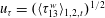
 $\mathit{Re}_{0}=u_{{\it\tau}}z_{0}/{\it\nu}$
, for ‘limiting’ values of the parameter range considered is
$\mathit{Re}_{0}=u_{{\it\tau}}z_{0}/{\it\nu}$
, for ‘limiting’ values of the parameter range considered is
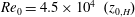 $\mathit{Re}_{0}=4.5\times 10^{4}~(z_{0,H})$
and
$\mathit{Re}_{0}=4.5\times 10^{4}~(z_{0,H})$
and
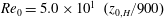 $\mathit{Re}_{0}=5.0\times 10^{1}~(z_{0,H}/900)$
, both of which satisfy the ‘fully rough’ condition,
$\mathit{Re}_{0}=5.0\times 10^{1}~(z_{0,H}/900)$
, both of which satisfy the ‘fully rough’ condition,
 $\mathit{Re}_{0}>2$
(Monin & Yaglom Reference Monin and Yaglom1971; Jimenez Reference Jimenez2004; Anderson Reference Anderson2013). To place these values in a boundary layer meteorology context,
$\mathit{Re}_{0}>2$
(Monin & Yaglom Reference Monin and Yaglom1971; Jimenez Reference Jimenez2004; Anderson Reference Anderson2013). To place these values in a boundary layer meteorology context,
 $z_{0}/{\it\delta}=10^{-3}$
corresponds to flows over urban environments while
$z_{0}/{\it\delta}=10^{-3}$
corresponds to flows over urban environments while
 $z_{0}/{\it\delta}\approx 1\times 10^{-6}$
corresponds to flows over gently undulating landscapes without any vegetation (Brutsaert Reference Brutsaert1982). We must emphasize that the cumulative effect of multiple roughness lengths on the same topography will – especially for the present cases – result in a highly perturbed mean flow that is not well characterized by
$z_{0}/{\it\delta}\approx 1\times 10^{-6}$
corresponds to flows over gently undulating landscapes without any vegetation (Brutsaert Reference Brutsaert1982). We must emphasize that the cumulative effect of multiple roughness lengths on the same topography will – especially for the present cases – result in a highly perturbed mean flow that is not well characterized by
 $z_{0,H}$
or
$z_{0,H}$
or
 $z_{0,L}$
(Bou-Zeid, Meneveau & Parlange Reference Bou-Zeid, Meneveau and Parlange2004; Bou-Zeid, Parlange & Meneveau Reference Bou-Zeid, Parlange and Meneveau2007). However, it is nonetheless worth while to see that the selected
$z_{0,L}$
(Bou-Zeid, Meneveau & Parlange Reference Bou-Zeid, Meneveau and Parlange2004; Bou-Zeid, Parlange & Meneveau Reference Bou-Zeid, Parlange and Meneveau2007). However, it is nonetheless worth while to see that the selected
 ${\it\lambda}$
values are based on realistic physical values. Since the LES code and associated averaging procedures necessary to retrieve distributions of Reynolds-stress tensor components are similar to a recent paper by the authors (Willingham et al.
Reference Willingham, Anderson, Christensen and Barros2013), we have placed details of the simulation procedures in appendix A. We note here however that
${\it\lambda}$
values are based on realistic physical values. Since the LES code and associated averaging procedures necessary to retrieve distributions of Reynolds-stress tensor components are similar to a recent paper by the authors (Willingham et al.
Reference Willingham, Anderson, Christensen and Barros2013), we have placed details of the simulation procedures in appendix A. We note here however that
 $\widetilde{\dots }$
denotes an LES grid-filtered quantity, vorticity is
$\widetilde{\dots }$
denotes an LES grid-filtered quantity, vorticity is
 $\tilde{{\it\omega}}_{i}=\{\tilde{{\it\omega}}_{1},\tilde{{\it\omega}}_{2},\tilde{{\it\omega}}_{3}\}$
, velocity is
$\tilde{{\it\omega}}_{i}=\{\tilde{{\it\omega}}_{1},\tilde{{\it\omega}}_{2},\tilde{{\it\omega}}_{3}\}$
, velocity is
 $\tilde{u} _{i}=\{\tilde{u} _{1},\tilde{u} _{2},\tilde{u} _{3}\}$
and spatial position is
$\tilde{u} _{i}=\{\tilde{u} _{1},\tilde{u} _{2},\tilde{u} _{3}\}$
and spatial position is
 $x_{i}=\{x_{1},x_{2},x_{3}\}$
, where indices
$x_{i}=\{x_{1},x_{2},x_{3}\}$
, where indices
 $i=1$
, 2 and 3 correspond to the streamwise, spanwise and vertical directions, respectively (this is shown also graphically in figure 1). Details of the experimental measurements are presented in appendix B.
$i=1$
, 2 and 3 correspond to the streamwise, spanwise and vertical directions, respectively (this is shown also graphically in figure 1). Details of the experimental measurements are presented in appendix B.
Table 1. Attributes of figure 1(b) topography for present LES cases.

We divided the present work as follows. Section 2 presents visualization of mean streamwise velocity and illustration of mean flow rotation associated with the centre of the LMP. We also present spanwise distributions of the imposed aerodynamic surface stress, which holds special importance in the underlying discussion of secondary flow generation mechanisms. This figure is contrasted against recent experimental results from Christensen and co-authors (Mejia-Alvarez et al.
Reference Mejia-Alvarez, Barros and Christensen2013; Mejia-Alvarez & Christensen Reference Mejia-Alvarez and Christensen2010, Reference Mejia-Alvarez and Christensen2013; Barros & Christensen Reference Barros and Christensen2014) for flow over the complex roughness (figure 1
a) with significant streamwise elongation and large-scale spanwise heterogeneity, and we report qualitative agreement with these experimental data. For additional details of the figure 1(a) topography, see appendix B. In § 3 we present turbulent normal and shearing stress components and
 $\mathit{tke}$
in the spanwise-wall normal plane, which demonstrates the presence of significant spatial variability due to the presence of the roughness. Section 4 focuses on studying the
$\mathit{tke}$
in the spanwise-wall normal plane, which demonstrates the presence of significant spatial variability due to the presence of the roughness. Section 4 focuses on studying the
 $\mathit{tke}$
transport equation and explaining why the mean secondary flow is necessary for preserving global energy conservation (Hinze Reference Hinze1967, Reference Hinze1973). Finally, in § 5 we use the Reynolds-stress distributions to study the production of mean streamwise vorticity and demonstrate that this quantity is predominantly produced in a region close to the roughness heterogeneity, consistent with our earlier suppositions (Willingham et al.
Reference Willingham, Anderson, Christensen and Barros2013). The findings in § 2 to § 5 demonstrate that the LMP and associated mean streamwise circulations are a realization of Prandtl’s secondary flow of the second kind. Section 6 presents a conclusion and summary of the work.
$\mathit{tke}$
transport equation and explaining why the mean secondary flow is necessary for preserving global energy conservation (Hinze Reference Hinze1967, Reference Hinze1973). Finally, in § 5 we use the Reynolds-stress distributions to study the production of mean streamwise vorticity and demonstrate that this quantity is predominantly produced in a region close to the roughness heterogeneity, consistent with our earlier suppositions (Willingham et al.
Reference Willingham, Anderson, Christensen and Barros2013). The findings in § 2 to § 5 demonstrate that the LMP and associated mean streamwise circulations are a realization of Prandtl’s secondary flow of the second kind. Section 6 presents a conclusion and summary of the work.

Figure 2. Visualization of time- and
 $x_{1}$
-averaged flow statistics for flow over
$x_{1}$
-averaged flow statistics for flow over
 ${\it\lambda}=2$
case (a,c), and from PIV results of boundary layer flow over a complex roughness reported in Barros & Christensen (Reference Barros and Christensen2014) (b,d). In (a,b), smooth contours are
${\it\lambda}=2$
case (a,c), and from PIV results of boundary layer flow over a complex roughness reported in Barros & Christensen (Reference Barros and Christensen2014) (b,d). In (a,b), smooth contours are
 $\langle \tilde{u} _{1}\rangle _{1,t}/u_{{\it\tau}}$
; and in (c,d), smooth contours are swirl strength,
$\langle \tilde{u} _{1}\rangle _{1,t}/u_{{\it\tau}}$
; and in (c,d), smooth contours are swirl strength,
 ${\it\Lambda}_{ci}$
, signed with mean streamwise vorticity (Zhou, Adrian & Balachandar Reference Zhou, Adrian and Balachandar1996; Zhou et al.
Reference Zhou, Adrian, Balachandar and Kendall1999; Adrian, Christensen & Liu Reference Adrian, Christensen and Liu2000a
; Mejia-Alvarez et al.
Reference Mejia-Alvarez, Barros and Christensen2013). In all panels, black vectors are components of spanwise and vertical velocity,
${\it\Lambda}_{ci}$
, signed with mean streamwise vorticity (Zhou, Adrian & Balachandar Reference Zhou, Adrian and Balachandar1996; Zhou et al.
Reference Zhou, Adrian, Balachandar and Kendall1999; Adrian, Christensen & Liu Reference Adrian, Christensen and Liu2000a
; Mejia-Alvarez et al.
Reference Mejia-Alvarez, Barros and Christensen2013). In all panels, black vectors are components of spanwise and vertical velocity,
 $\{\langle \tilde{u} _{2}\rangle _{1,t}/u_{{\it\tau}},\langle \tilde{u} _{3}\rangle _{1,t}/u_{{\it\tau}}\}$
. Solid vertical black lines show centre of LMP and HMP, where specific structure is labelled at top of each panel. In (a,c), dashed vertical black line denotes spanwise position of aerodynamic roughness step change for figure 1(a) topography. In (b,d), the solid black profile at bottom is low-pass-filtered spanwise roughness height,
$\{\langle \tilde{u} _{2}\rangle _{1,t}/u_{{\it\tau}},\langle \tilde{u} _{3}\rangle _{1,t}/u_{{\it\tau}}\}$
. Solid vertical black lines show centre of LMP and HMP, where specific structure is labelled at top of each panel. In (a,c), dashed vertical black line denotes spanwise position of aerodynamic roughness step change for figure 1(a) topography. In (b,d), the solid black profile at bottom is low-pass-filtered spanwise roughness height,
 ${\it\eta}$
(a,c), computed from a
${\it\eta}$
(a,c), computed from a
 ${\it\delta}$
-long streamwise average of roughness height upstream of the measurement plane as reported by Willingham et al. (Reference Willingham, Anderson, Christensen and Barros2013) and Barros & Christensen (Reference Barros and Christensen2014). The solid grey profile is spanwise gradient of
${\it\delta}$
-long streamwise average of roughness height upstream of the measurement plane as reported by Willingham et al. (Reference Willingham, Anderson, Christensen and Barros2013) and Barros & Christensen (Reference Barros and Christensen2014). The solid grey profile is spanwise gradient of
 ${\it\eta}$
, illustrating where abrupt changes in low-pass-filtered height occur. Note that all following spanwise-wall normal contours of turbulence statistics from LES and PIV experiments include these lines and profiles. Also, in this paper, a blue–yellow–red colour scheme is adopted for illustrating quantities exhibiting values all of equal sign (a,b), above), while a blue–white–red colour scheme is adopted for quantities exhibiting a mean of zero (as is the case for (c,d), above).
${\it\eta}$
, illustrating where abrupt changes in low-pass-filtered height occur. Note that all following spanwise-wall normal contours of turbulence statistics from LES and PIV experiments include these lines and profiles. Also, in this paper, a blue–yellow–red colour scheme is adopted for illustrating quantities exhibiting values all of equal sign (a,b), above), while a blue–white–red colour scheme is adopted for quantities exhibiting a mean of zero (as is the case for (c,d), above).
2. Turbulent secondary flow
Figure 2(a) illustrates time-averaged velocity components (contours, streamwise; vectors, spanwise-wall normal components) in the spanwise-wall normal plane from an LES at
 ${\it\lambda}=2$
and shows a
${\it\lambda}=2$
and shows a
 ${\it\delta}$
-scale zone of low-momentum fluid in the mean flow, centred roughly midway between the two high-roughness strips (roughness transitions denoted by vertical dashed black line). This zone constitutes a low-momentum pathway, as defined by Mejia-Alvarez & Christensen (Reference Mejia-Alvarez and Christensen2013) and Barros & Christensen (Reference Barros and Christensen2014). The reported flow heterogeneity is a time-invariant attribute and not the product of an inadequately short time-averaging period. This flow pattern occurred for all
${\it\delta}$
-scale zone of low-momentum fluid in the mean flow, centred roughly midway between the two high-roughness strips (roughness transitions denoted by vertical dashed black line). This zone constitutes a low-momentum pathway, as defined by Mejia-Alvarez & Christensen (Reference Mejia-Alvarez and Christensen2013) and Barros & Christensen (Reference Barros and Christensen2014). The reported flow heterogeneity is a time-invariant attribute and not the product of an inadequately short time-averaging period. This flow pattern occurred for all
 ${\it\lambda}$
values considered in this study (not shown for brevity; see also Willingham et al. (Reference Willingham, Anderson, Christensen and Barros2013) for additional visualization for different
${\it\lambda}$
values considered in this study (not shown for brevity; see also Willingham et al. (Reference Willingham, Anderson, Christensen and Barros2013) for additional visualization for different
 ${\it\lambda}$
and
${\it\lambda}$
and
 $L_{s}/{\it\delta}$
values). The LMP is flanked by mean flow counter-rotating vortices that converge roughly at the bottom of the LMP. More striking still is the observation that low- and high-momentum fluid occupies the region above the low and high roughness, respectively. The streamwise-aligned roll motions, illustrated by vectors of
$L_{s}/{\it\delta}$
values). The LMP is flanked by mean flow counter-rotating vortices that converge roughly at the bottom of the LMP. More striking still is the observation that low- and high-momentum fluid occupies the region above the low and high roughness, respectively. The streamwise-aligned roll motions, illustrated by vectors of
 $\{\langle \tilde{u} _{2}\rangle _{1,t}/u_{{\it\tau}},\langle \tilde{u} _{3}\rangle _{1,t}/u_{{\it\tau}}\}$
, are systematically redistributing momentum throughout the domain in response to the imposed surface drag and local non-equilibrium between production and dissipation of
$\{\langle \tilde{u} _{2}\rangle _{1,t}/u_{{\it\tau}},\langle \tilde{u} _{3}\rangle _{1,t}/u_{{\it\tau}}\}$
, are systematically redistributing momentum throughout the domain in response to the imposed surface drag and local non-equilibrium between production and dissipation of
 $\mathit{tke}$
(discussion to follow in § 4). Figure 2(c) shows contours of swirl strength,
$\mathit{tke}$
(discussion to follow in § 4). Figure 2(c) shows contours of swirl strength,
 ${\it\Lambda}_{ci}$
, which is here computed as the imaginary component of the complex eigenvalue of the two-dimensional (spanwise-wall normal) velocity gradient tensor,
${\it\Lambda}_{ci}$
, which is here computed as the imaginary component of the complex eigenvalue of the two-dimensional (spanwise-wall normal) velocity gradient tensor,
 $$\begin{eqnarray}\unicode[STIX]{x1D60B}_{23}=\left[\begin{array}{@{}cc@{}}{\displaystyle \frac{\partial \langle \tilde{u} _{2}\rangle _{1,t}}{\partial x_{2}}} & {\displaystyle \frac{\partial \langle \tilde{u} _{2}\rangle _{1,t}}{\partial x_{3}}}\\ {\displaystyle \frac{\partial \langle \tilde{u} _{3}\rangle _{1,t}}{\partial x_{2}}} & {\displaystyle \frac{\partial \langle \tilde{u} _{3}\rangle _{1,t}}{\partial x_{3}}}\end{array}\right],\end{eqnarray}$$
though here we follow Wu & Christensen (Reference Wu and Christensen2006) by assigning polarity of
 ${\it\Lambda}_{ci}$
based on the local in-plane vorticity,
${\it\Lambda}_{ci}$
based on the local in-plane vorticity,
 $\langle \tilde{{\it\omega}}\rangle _{1,t}=\partial \langle \tilde{u} _{3}\rangle _{1,t}/\partial x_{2}-\partial \langle \tilde{u} _{2}\rangle _{1,t}/\partial x_{3}$
. Thus, a signed swirl strength is obtained,
$\langle \tilde{{\it\omega}}\rangle _{1,t}=\partial \langle \tilde{u} _{3}\rangle _{1,t}/\partial x_{2}-\partial \langle \tilde{u} _{2}\rangle _{1,t}/\partial x_{3}$
. Thus, a signed swirl strength is obtained,
 ${\it\Lambda}_{ci}\rightarrow {\it\Lambda}_{ci}(\langle \tilde{{\it\omega}}\rangle _{1,t}/\Vert \langle \tilde{{\it\omega}}\rangle _{1,t}\Vert )$
, enabling one to infer that
${\it\Lambda}_{ci}\rightarrow {\it\Lambda}_{ci}(\langle \tilde{{\it\omega}}\rangle _{1,t}/\Vert \langle \tilde{{\it\omega}}\rangle _{1,t}\Vert )$
, enabling one to infer that
 ${\it\Lambda}_{ci}<0$
,
${\it\Lambda}_{ci}<0$
,
 ${\it\Lambda}_{ci}=0$
and
${\it\Lambda}_{ci}=0$
and
 ${\it\Lambda}_{ci}>0$
correspond to negative (anticlockwise) rotation, no rotation and positive (clockwise) rotation of the mean streamwise vorticity, respectively. Thus, figure 2(c) illustrates the presence of mean
${\it\Lambda}_{ci}>0$
correspond to negative (anticlockwise) rotation, no rotation and positive (clockwise) rotation of the mean streamwise vorticity, respectively. Thus, figure 2(c) illustrates the presence of mean
 ${\it\delta}$
-scale circulating cells associated with upwelling (
${\it\delta}$
-scale circulating cells associated with upwelling (
 $\langle \tilde{u} _{3}\rangle _{1,t}>0$
) and downwelling (
$\langle \tilde{u} _{3}\rangle _{1,t}>0$
) and downwelling (
 $\langle \tilde{u} _{3}\rangle _{1,t}<0$
) within the LMP and HMP, respectively.
$\langle \tilde{u} _{3}\rangle _{1,t}<0$
) within the LMP and HMP, respectively.
The LMPs and HMPs are systematically positioned above the low- and high-roughness regions, respectively (see figure 1
b), and this suggests that such a roughness configuration could be used to impart large-scale features in the flow. The figure 1(b) topography is an idealistic limiting case, which is appropriate for studying LMP and HMP physics in a controlled setting. However, figure 2(b,d) shows results from the Laboratory for Turbulence and Complex Flow at the University of Illinois at Urbana-Champaign for flow over the figure 1(a) topography (see also Barros & Christensen Reference Barros and Christensen2014). Appendix B presents a brief description of the experimental facility at which the measurements were made. The figure shows mean flow motions that are strikingly similar to those observed in the controlled LES case, though the topography considered embodies a broad range of roughness scales. Despite this topographical complexity, large-scale spanwise heterogeneity in this complex roughness is noted in the spanwise roughness profile shown beneath the experimental data in figure 2(b,d) computed by streamwise averaging the roughness profile one
 ${\it\delta}$
upstream of the measurement position and low-pass-filtered to highlight its large-scale spanwise heterogeneity (see also Barros & Christensen Reference Barros and Christensen2014). In fact, the solid grey profile beneath figure 2(b,d) shows the spanwise gradient in roughness height (
${\it\delta}$
upstream of the measurement position and low-pass-filtered to highlight its large-scale spanwise heterogeneity (see also Barros & Christensen Reference Barros and Christensen2014). In fact, the solid grey profile beneath figure 2(b,d) shows the spanwise gradient in roughness height (
 $\partial {\it\eta}/\partial x_{2}$
; grey line) computed from the spanwise roughness profile,
$\partial {\it\eta}/\partial x_{2}$
; grey line) computed from the spanwise roughness profile,
 ${\it\eta}$
. Focusing upon the mean velocity field in figure 2(b), LMP signatures are readily apparent at spanwise locations of relatively recessed roughness while HMPs reside at spanwise locations of relatively elevated roughness in these experimental results, with counter-rotating swirling motions bounding these regions. Consider the clear ‘downwelling’ (negative mean vertical velocity) at
${\it\eta}$
. Focusing upon the mean velocity field in figure 2(b), LMP signatures are readily apparent at spanwise locations of relatively recessed roughness while HMPs reside at spanwise locations of relatively elevated roughness in these experimental results, with counter-rotating swirling motions bounding these regions. Consider the clear ‘downwelling’ (negative mean vertical velocity) at
 $x_{2}/{\it\delta}\approx -1$
and
$x_{2}/{\it\delta}\approx -1$
and
 $-0.25$
; similarly we see strong ‘upwelling’ (positive mean vertical velocity) at
$-0.25$
; similarly we see strong ‘upwelling’ (positive mean vertical velocity) at
 $x_{2}/{\it\delta}\approx 0.9$
, 0.2 and
$x_{2}/{\it\delta}\approx 0.9$
, 0.2 and
 $-0.6$
. Consultation of the below streamwise-averaged complex roughness height illustrates the strong correlation of these HMPs and LMPs with relative topographic peaks and troughs, respectively, as well as spanwise locations of
$-0.6$
. Consultation of the below streamwise-averaged complex roughness height illustrates the strong correlation of these HMPs and LMPs with relative topographic peaks and troughs, respectively, as well as spanwise locations of
 $\partial {\it\eta}/\partial x_{2}\approx 0$
. The agreement is, of course, not nearly as direct as observed for the LES cases, owing to the inherent complexity of the topography. Rather, qualitative agreement between the experimental and numerical datasets motivates this study, since elucidating trends for the idealized (LES) case aids in understanding flow patterns present for the complex (experimental) case.
$\partial {\it\eta}/\partial x_{2}\approx 0$
. The agreement is, of course, not nearly as direct as observed for the LES cases, owing to the inherent complexity of the topography. Rather, qualitative agreement between the experimental and numerical datasets motivates this study, since elucidating trends for the idealized (LES) case aids in understanding flow patterns present for the complex (experimental) case.

Figure 3. Profiles of
 $x_{1}$
- and time-averaged imposed aerodynamic wall stress computed with (A 3): (a)
$x_{1}$
- and time-averaged imposed aerodynamic wall stress computed with (A 3): (a)
 $i=1$
; (b)
$i=1$
; (b)
 $i=2$
. Profiles correspond to
$i=2$
. Profiles correspond to
 ${\it\lambda}=2$
(solid black),
${\it\lambda}=2$
(solid black),
 ${\it\lambda}=10$
(dashed black),
${\it\lambda}=10$
(dashed black),
 ${\it\lambda}=25$
(solid dark grey),
${\it\lambda}=25$
(solid dark grey),
 ${\it\lambda}=100$
(dashed dark grey),
${\it\lambda}=100$
(dashed dark grey),
 ${\it\lambda}=500$
(solid light grey),
${\it\lambda}=500$
(solid light grey),
 ${\it\lambda}=900$
(dashed light grey), homogeneous
${\it\lambda}=900$
(dashed light grey), homogeneous
 $z_{0}/H=10^{-3}$
(solid black with black circles).
$z_{0}/H=10^{-3}$
(solid black with black circles).
It should also be noted that the spanwise locations of the mean flow swirling motions tend to coincide with large-scale spanwise gradients in the topography, specifically mean clockwise swirl when
 $\partial {\it\eta}/\partial x_{2}>0$
(due to local transitions in relative topographical height from recessed to elevated in the positive
$\partial {\it\eta}/\partial x_{2}>0$
(due to local transitions in relative topographical height from recessed to elevated in the positive
 $x_{2}$
direction) and mean anticlockwise swirl when
$x_{2}$
direction) and mean anticlockwise swirl when
 $\partial {\it\eta}/\partial x_{2}<0$
(due to local transitions in relative topographical height from elevated to recessed in the positive
$\partial {\it\eta}/\partial x_{2}<0$
(due to local transitions in relative topographical height from elevated to recessed in the positive
 $x_{2}$
direction). Specifically focusing on the LMP that resides near
$x_{2}$
direction). Specifically focusing on the LMP that resides near
 $x_{2}/{\it\delta}\approx 0.15$
(figure 2
b,d), it is bounded by mean anticlockwise swirl at
$x_{2}/{\it\delta}\approx 0.15$
(figure 2
b,d), it is bounded by mean anticlockwise swirl at
 $x_{2}/{\it\delta}\approx 0$
(coincident with
$x_{2}/{\it\delta}\approx 0$
(coincident with
 $\partial {\it\eta}/\partial x_{2}<0$
) and mean clockwise swirl at
$\partial {\it\eta}/\partial x_{2}<0$
) and mean clockwise swirl at
 $x_{2}/{\it\delta}\approx 0.35$
(coincident with
$x_{2}/{\it\delta}\approx 0.35$
(coincident with
 $\partial {\it\eta}/\partial x_{2}>0$
). All of these spatial characteristics are quite consistent with the patterns noted in the more controlled LES roughness cases and suggest that even subtle spanwise heterogeneity in roughness topography can generate and sustain
$\partial {\it\eta}/\partial x_{2}>0$
). All of these spatial characteristics are quite consistent with the patterns noted in the more controlled LES roughness cases and suggest that even subtle spanwise heterogeneity in roughness topography can generate and sustain
 ${\it\delta}$
-scale mean flow heterogeneities. While spanwise mirroring of the complex roughness was required in order to fill the entire span of the wind tunnel with roughness (in approximately
${\it\delta}$
-scale mean flow heterogeneities. While spanwise mirroring of the complex roughness was required in order to fill the entire span of the wind tunnel with roughness (in approximately
 $3{\it\delta}$
increments in the span; see appendix B), the spanwise field of view presented in figure 2(b,d) occurs over a unique spanwise portion of the original roughness. Thus, the flow physics presented in these figures occurs over roughness that is not impacted by the need to mirror the original topography in the spanwise direction.
$3{\it\delta}$
increments in the span; see appendix B), the spanwise field of view presented in figure 2(b,d) occurs over a unique spanwise portion of the original roughness. Thus, the flow physics presented in these figures occurs over roughness that is not impacted by the need to mirror the original topography in the spanwise direction.
We note that these secondary flow patterns are qualitatively consistent with observations of turbulent flows in ducts (as reviewed briefly in § 1). Since imposed surface stress (see appendix A) is thought to be inherently responsible for sustaining the LMP–HMP flow heterogeneity, we consider figure 3(a), which shows the stress distributions for all six LES cases described in table 1 (in addition to results of flow over a homogeneous roughness, which by conservation of momentum must be
 $\langle {\it\tau}_{13}^{w}\rangle _{1,t}/u_{{\it\tau}}^{2}=-1$
). Inclusion of the homogeneous roughness case (which is equivalent to
$\langle {\it\tau}_{13}^{w}\rangle _{1,t}/u_{{\it\tau}}^{2}=-1$
). Inclusion of the homogeneous roughness case (which is equivalent to
 ${\it\lambda}=1$
) facilitates inspection of the role of
${\it\lambda}=1$
) facilitates inspection of the role of
 ${\it\lambda}>1$
, and we observe
${\it\lambda}>1$
, and we observe
 $\langle {\it\tau}_{13}^{w}\rangle _{1,t}/u_{{\it\tau}}^{2}$
decreasing (‘bigger negative’) monotonically with increasing
$\langle {\it\tau}_{13}^{w}\rangle _{1,t}/u_{{\it\tau}}^{2}$
decreasing (‘bigger negative’) monotonically with increasing
 ${\it\lambda}$
, demonstrating that the
${\it\lambda}$
, demonstrating that the
 $z_{0,H}$
and
$z_{0,H}$
and
 $z_{0,L}$
regions of the roughness absorb progressively more and less momentum, respectively, as
$z_{0,L}$
regions of the roughness absorb progressively more and less momentum, respectively, as
 ${\it\lambda}$
increases. Since momentum conservation is preserved and the logarithmic law (A 3) serves to maintain equilibrium with the imposed pressure gradient forcing,
${\it\lambda}$
increases. Since momentum conservation is preserved and the logarithmic law (A 3) serves to maintain equilibrium with the imposed pressure gradient forcing,
 ${\it\Pi}$
, in (A 1), figure 3 illustrates a redistribution of drag with increasing
${\it\Pi}$
, in (A 1), figure 3 illustrates a redistribution of drag with increasing
 ${\it\lambda}$
. The
${\it\lambda}$
. The
 $\langle {\it\tau}_{23}^{w}\rangle _{1,t}/u_{{\it\tau}}^{2}$
profiles in figure 3(b) show deviations about zero due to the spanwise component of the mean secondary flow,
$\langle {\it\tau}_{23}^{w}\rangle _{1,t}/u_{{\it\tau}}^{2}$
profiles in figure 3(b) show deviations about zero due to the spanwise component of the mean secondary flow,
 $\tilde{u} _{2}/u_{{\it\tau}}$
. Equation (A 3) shows that surface stress imposed with the equilibrium logarithmic law,
$\tilde{u} _{2}/u_{{\it\tau}}$
. Equation (A 3) shows that surface stress imposed with the equilibrium logarithmic law,
 $\langle {\it\tau}_{i3}^{w}\rangle _{1,t}/u_{{\it\tau}}^{2}~(i=1,2)$
, is effectively set by the
$\langle {\it\tau}_{i3}^{w}\rangle _{1,t}/u_{{\it\tau}}^{2}~(i=1,2)$
, is effectively set by the
 $i$
th velocity component,
$i$
th velocity component,
 $\tilde{u} _{i}/u_{{\it\tau}}$
. Figure 2(a) showed that
$\tilde{u} _{i}/u_{{\it\tau}}$
. Figure 2(a) showed that
 $\tilde{u} _{2}/u_{{\it\tau}}$
associated with the counter-rotating vortices induces flow laterally ‘off’ the
$\tilde{u} _{2}/u_{{\it\tau}}$
associated with the counter-rotating vortices induces flow laterally ‘off’ the
 $z_{0,H}$
strips. This explains the variability (and symmetry) of the
$z_{0,H}$
strips. This explains the variability (and symmetry) of the
 $\langle {\it\tau}_{23}^{w}\rangle _{1,t}/u_{{\it\tau}}^{2}$
profiles reported in figure 3.
$\langle {\it\tau}_{23}^{w}\rangle _{1,t}/u_{{\it\tau}}^{2}$
profiles reported in figure 3.
As an aside, we note Sheng, Malkiel & Katz (Reference Sheng, Malkiel and Katz2009), who experimentally investigated the relationships between imposed surface stress and coherent turbulent morphologies present in turbulent boundary layer flow over a smooth wall. They reported that the presence of horseshoe vortices and associated quasi-streamwise vorticity due to counter-rotating hairpin legs exhibited close correlation to imposed surface stress variations. Specifically, they showed that surface stress is locally small at the hairpin origin. Adjacent (and slightly staggered in the streamwise direction) to these relative drag deficits are emergent peaks of surface stress. The local minimum in imposed surface stress beneath the hairpin vortex head is persistent and is a result of the predominant contribution made by turbulent ejections due to these structures (positive and negative vertical and streamwise velocity fluctuations, respectively). Thus, the LMRs and LMPs are flanked by counter-rotating vortices of equivalent sign (see Sheng et al. Reference Sheng, Malkiel and Katz2009 and figure 2 a,b). In addition, we have reported that imposed surface stress is lowest beneath the LMPs, which is qualitatively similar to LMRs (figure 3 a). Willingham et al. (Reference Willingham, Anderson, Christensen and Barros2013) provided discussion on the role of the spanwise stress distribution (figure 3) for the figure 1(a) roughness; it is important to study now the resultant Reynolds stresses and tke, since spanwise-wall normal heterogeneities of these quantities sustain the figure 2 secondary flow.

Figure 4. Contours of turbulent (Reynolds) stresses and turbulent kinetic energy,
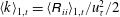 $\langle k\rangle _{1,t}=\langle \unicode[STIX]{x1D619}_{ii}\rangle _{1,t}/u_{{\it\tau}}^{2}/2$
, for (a,c,e,g,i,k,m) LES case with
$\langle k\rangle _{1,t}=\langle \unicode[STIX]{x1D619}_{ii}\rangle _{1,t}/u_{{\it\tau}}^{2}/2$
, for (a,c,e,g,i,k,m) LES case with
 ${\it\lambda}=2$
and (b,d, f,h, j,l,n) experimental case (see also Barros & Christensen Reference Barros and Christensen2014): (a,b)
${\it\lambda}=2$
and (b,d, f,h, j,l,n) experimental case (see also Barros & Christensen Reference Barros and Christensen2014): (a,b)
 $\langle \unicode[STIX]{x1D619}_{11}\rangle _{1,t}/u_{{\it\tau}}^{2}$
; (c,d)
$\langle \unicode[STIX]{x1D619}_{11}\rangle _{1,t}/u_{{\it\tau}}^{2}$
; (c,d)
 $\langle \unicode[STIX]{x1D619}_{13}\rangle _{1,t}/u_{{\it\tau}}^{2}$
; (e, f)
$\langle \unicode[STIX]{x1D619}_{13}\rangle _{1,t}/u_{{\it\tau}}^{2}$
; (e, f)
 $\langle \unicode[STIX]{x1D619}_{22}\rangle _{1,t}/u_{{\it\tau}}^{2}$
; (g,h)
$\langle \unicode[STIX]{x1D619}_{22}\rangle _{1,t}/u_{{\it\tau}}^{2}$
; (g,h)
 $\langle \unicode[STIX]{x1D619}_{23}\rangle _{1,t}/u_{{\it\tau}}^{2}$
; (i, j)
$\langle \unicode[STIX]{x1D619}_{23}\rangle _{1,t}/u_{{\it\tau}}^{2}$
; (i, j)
 $\langle \unicode[STIX]{x1D619}_{33}\rangle _{1,t}/u_{{\it\tau}}^{2}$
; (k,l)
$\langle \unicode[STIX]{x1D619}_{33}\rangle _{1,t}/u_{{\it\tau}}^{2}$
; (k,l)
 $\langle \unicode[STIX]{x1D619}_{12}\rangle _{1,t}/u_{{\it\tau}}^{2}$
; and (m,n)
$\langle \unicode[STIX]{x1D619}_{12}\rangle _{1,t}/u_{{\it\tau}}^{2}$
; and (m,n)
 $\langle k\rangle _{1,t}$
. The friction velocity is set as
$\langle k\rangle _{1,t}$
. The friction velocity is set as
 $u_{{\it\tau}}=(\langle {\it\tau}_{13}^{w}\rangle _{1,2,t})^{1/2}$
.
$u_{{\it\tau}}=(\langle {\it\tau}_{13}^{w}\rangle _{1,2,t})^{1/2}$
.
3. Turbulence statistics
Figure 4 shows the components of the Reynolds-stress tensor,
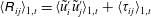 $\langle \unicode[STIX]{x1D619}_{ij}\rangle _{1,t}=\langle \tilde{u} _{i}^{\prime }\tilde{u} _{j}^{\prime }\rangle _{1,t}+\langle {\it\tau}_{ij}\rangle _{1,t}$
, for the LES topography (figure 4
a,c,e,g,i,k) and experimental topography (figure 4
b,d, f,h, j,l). The LES case corresponds to
$\langle \unicode[STIX]{x1D619}_{ij}\rangle _{1,t}=\langle \tilde{u} _{i}^{\prime }\tilde{u} _{j}^{\prime }\rangle _{1,t}+\langle {\it\tau}_{ij}\rangle _{1,t}$
, for the LES topography (figure 4
a,c,e,g,i,k) and experimental topography (figure 4
b,d, f,h, j,l). The LES case corresponds to
 ${\it\lambda}=2$
(see (A 4) for discussion of retrieving total turbulent stresses from LES statistics). It is clear from figure 4(a,c,e,g,i,k) that spatial heterogeneity exists in the turbulent stress distributions that are far different from what would otherwise be present for flow over a homogeneous roughness or a smooth wall. The normal stresses (figure 4
a,c,e) exhibit maximum values above the high-roughness strip, close to the wall. Interestingly, however, we see a wall-normal attenuation of the normal stresses to values far lower than in the adjacent LMP region (i.e. for
${\it\lambda}=2$
(see (A 4) for discussion of retrieving total turbulent stresses from LES statistics). It is clear from figure 4(a,c,e,g,i,k) that spatial heterogeneity exists in the turbulent stress distributions that are far different from what would otherwise be present for flow over a homogeneous roughness or a smooth wall. The normal stresses (figure 4
a,c,e) exhibit maximum values above the high-roughness strip, close to the wall. Interestingly, however, we see a wall-normal attenuation of the normal stresses to values far lower than in the adjacent LMP region (i.e. for
 $x_{3}/{\it\delta}\gtrsim 1/3$
). Moreover, owing to the spanwise-vertical secondary mean flow, we see elevated normal stresses within the LMP for
$x_{3}/{\it\delta}\gtrsim 1/3$
). Moreover, owing to the spanwise-vertical secondary mean flow, we see elevated normal stresses within the LMP for
 $x_{3}/{\it\delta}\gtrsim 0.3$
relative to the adjacent HMPs. Figure 4(g,i,k) shows the shearing stress components and we see important spanwise variations of these stresses. Figure 4(i) illustrates that the largest
$x_{3}/{\it\delta}\gtrsim 0.3$
relative to the adjacent HMPs. Figure 4(g,i,k) shows the shearing stress components and we see important spanwise variations of these stresses. Figure 4(i) illustrates that the largest
 $\unicode[STIX]{x1D619}_{13}$
occurs at the base of the HMP and this manifests also in figure 3(a) (largest drag on the high-roughness strip). However, we again see that within the HMP the wall-normal attenuation of
$\unicode[STIX]{x1D619}_{13}$
occurs at the base of the HMP and this manifests also in figure 3(a) (largest drag on the high-roughness strip). However, we again see that within the HMP the wall-normal attenuation of
 $\langle \unicode[STIX]{x1D619}_{13}\rangle _{1,t}/u_{{\it\tau}}^{2}$
is large and this value reaches its minimum at an elevation lower than in the adjacent LMP. The
$\langle \unicode[STIX]{x1D619}_{13}\rangle _{1,t}/u_{{\it\tau}}^{2}$
is large and this value reaches its minimum at an elevation lower than in the adjacent LMP. The
 $\langle \unicode[STIX]{x1D619}_{23}\rangle _{1,t}/u_{{\it\tau}}^{2}$
stress distribution exhibits digression from zero with the same sign as streamwise vorticity (see also figure 2
c). The limits of
$\langle \unicode[STIX]{x1D619}_{23}\rangle _{1,t}/u_{{\it\tau}}^{2}$
stress distribution exhibits digression from zero with the same sign as streamwise vorticity (see also figure 2
c). The limits of
 $\langle \unicode[STIX]{x1D619}_{23}\rangle _{1,t}/u_{{\it\tau}}^{2}$
are roughly an order of magnitude smaller than the other stress components; however, it will be shown in the following sections (§§ 4 and 5) that it is spatial gradients of these quantities that are responsible for producing the underlying mean secondary flow and mean streamwise vorticity. Finally, figure 4(k) shows the
$\langle \unicode[STIX]{x1D619}_{23}\rangle _{1,t}/u_{{\it\tau}}^{2}$
are roughly an order of magnitude smaller than the other stress components; however, it will be shown in the following sections (§§ 4 and 5) that it is spatial gradients of these quantities that are responsible for producing the underlying mean secondary flow and mean streamwise vorticity. Finally, figure 4(k) shows the
 $\langle \unicode[STIX]{x1D619}_{12}\rangle _{1,t}/u_{{\it\tau}}^{2}$
shearing stress, which we (Willingham et al.
Reference Willingham, Anderson, Christensen and Barros2013) have previously studied for its role in sustaining lateral momentum exchange in close proximity to the roughness heterogeneity. The polarity of
$\langle \unicode[STIX]{x1D619}_{12}\rangle _{1,t}/u_{{\it\tau}}^{2}$
shearing stress, which we (Willingham et al.
Reference Willingham, Anderson, Christensen and Barros2013) have previously studied for its role in sustaining lateral momentum exchange in close proximity to the roughness heterogeneity. The polarity of
 $\langle \unicode[STIX]{x1D619}_{12}\rangle _{1,t}/u_{{\it\tau}}^{2}$
is consistent with the spanwise variation of mean streamwise velocity, and illustrates the presence of vertical shearing layers present in the flow (Vermaas et al.
Reference Vermaas, Uijttewall and Hoitink2011; Willingham et al.
Reference Willingham, Anderson, Christensen and Barros2013).
$\langle \unicode[STIX]{x1D619}_{12}\rangle _{1,t}/u_{{\it\tau}}^{2}$
is consistent with the spanwise variation of mean streamwise velocity, and illustrates the presence of vertical shearing layers present in the flow (Vermaas et al.
Reference Vermaas, Uijttewall and Hoitink2011; Willingham et al.
Reference Willingham, Anderson, Christensen and Barros2013).
For effectively all
 $x_{3}$
, there are local finite values of
$x_{3}$
, there are local finite values of
 $\langle \unicode[STIX]{x1D619}_{12}\rangle _{1,t}/u_{{\it\tau}}^{2}$
that are associated with the spanwise mean (streamwise) flow gradient induced by the LMP–HMP transition (figure 2(a) also reflects this). Similar patterns exist in the Reynolds-stress components from the experimental results for flow over complex roughness (figure 4
b,d, f,h, j,l) wherein the stereo particle image velocimetry (PIV) measurements in the cross-plane allowed calculation of all six Reynolds-stress components. Moreover, this figure includes indication of the low-pass-filtered
$\langle \unicode[STIX]{x1D619}_{12}\rangle _{1,t}/u_{{\it\tau}}^{2}$
that are associated with the spanwise mean (streamwise) flow gradient induced by the LMP–HMP transition (figure 2(a) also reflects this). Similar patterns exist in the Reynolds-stress components from the experimental results for flow over complex roughness (figure 4
b,d, f,h, j,l) wherein the stereo particle image velocimetry (PIV) measurements in the cross-plane allowed calculation of all six Reynolds-stress components. Moreover, this figure includes indication of the low-pass-filtered
 ${\it\delta}$
-long streamwise-averaged complex roughness height, which serves to provide qualitative representation of imposed aerodynamic stress. It is again evident that the largest
${\it\delta}$
-long streamwise-averaged complex roughness height, which serves to provide qualitative representation of imposed aerodynamic stress. It is again evident that the largest
 $\unicode[STIX]{x1D619}_{13}$
occurs closest to the high-drag region, at the base of HMPs, while elevated stresses are also present higher in the domain within the HMPs. Incidentally, these distributions of
$\unicode[STIX]{x1D619}_{13}$
occurs closest to the high-drag region, at the base of HMPs, while elevated stresses are also present higher in the domain within the HMPs. Incidentally, these distributions of
 $\unicode[STIX]{x1D619}_{ij}$
are precisely consistent with earlier observations reported by Wang & Cheng (Reference Wang and Cheng2005), who demonstrated indeed that
$\unicode[STIX]{x1D619}_{ij}$
are precisely consistent with earlier observations reported by Wang & Cheng (Reference Wang and Cheng2005), who demonstrated indeed that
 $\unicode[STIX]{x1D619}_{13}$
exhibits its maxima and minima at the base and top of the HMP, respectively (although the HMP and LMP nomenclature had not been introduced at that time).
$\unicode[STIX]{x1D619}_{13}$
exhibits its maxima and minima at the base and top of the HMP, respectively (although the HMP and LMP nomenclature had not been introduced at that time).
The
 $\mathit{tke}$
distribution for
$\mathit{tke}$
distribution for
 ${\it\lambda}=2$
is shown in figure 4(m). The figure is consistent with the normal stress distributions shown in figure 4(a,c,e); the maximum and minimum values of
${\it\lambda}=2$
is shown in figure 4(m). The figure is consistent with the normal stress distributions shown in figure 4(a,c,e); the maximum and minimum values of
 $\mathit{tke}$
clearly occur within the HMP closest and farthest from the wall, respectively. For
$\mathit{tke}$
clearly occur within the HMP closest and farthest from the wall, respectively. For
 $x_{3}/{\it\delta}\gtrsim 0.25$
,
$x_{3}/{\it\delta}\gtrsim 0.25$
,
 $\mathit{tke}$
is larger within the LMP. This is precisely consistent with the complementary experimental
$\mathit{tke}$
is larger within the LMP. This is precisely consistent with the complementary experimental
 $\mathit{tke}$
results (figure 4
n) and is an outcome of the turbulent secondary flows that are redistributing
$\mathit{tke}$
results (figure 4
n) and is an outcome of the turbulent secondary flows that are redistributing
 $\mathit{tke}$
as a result of gradients in the Reynolds stresses. We emphasize that the figure 4 flow patterns are observed for other
$\mathit{tke}$
as a result of gradients in the Reynolds stresses. We emphasize that the figure 4 flow patterns are observed for other
 ${\it\lambda}$
values considered in the present study, but we omit them here for brevity. We specifically have selected
${\it\lambda}$
values considered in the present study, but we omit them here for brevity. We specifically have selected
 ${\it\lambda}=2$
since this corresponds to the weakest difference between the ‘low’ and ‘high’ roughness considered and yet the turbulent secondary flow patterns are clearly present and the qualitative agreement with experimental patterns is strong.
${\it\lambda}=2$
since this corresponds to the weakest difference between the ‘low’ and ‘high’ roughness considered and yet the turbulent secondary flow patterns are clearly present and the qualitative agreement with experimental patterns is strong.
4. Mechanical energy balance and secondary flow pattern
The previous sections demonstrated significant spanwise-wall normal heterogeneity in the time-averaged streamwise velocity and Reynolds stresses, and this is integral to identifying underlying production mechanisms responsible for sustaining the secondary flow. Here we advance the analysis of the problem by studying terms present in the Reynolds-averaged
 $\mathit{tke}$
transport equation. In this section we demonstrate that spatial (
$\mathit{tke}$
transport equation. In this section we demonstrate that spatial (
 $x_{2}$
–
$x_{2}$
–
 $x_{3}$
plane) variation of
$x_{3}$
plane) variation of
 $\mathit{tke}$
production by mean flow gradients beyond the wall-normal gradient present in a boundary layer sustain the secondary flow. The secondary flow and local non-equilibrium between production and dissipation are shown to necessarily induce advection of
$\mathit{tke}$
production by mean flow gradients beyond the wall-normal gradient present in a boundary layer sustain the secondary flow. The secondary flow and local non-equilibrium between production and dissipation are shown to necessarily induce advection of
 $\mathit{tke}$
. As will be seen below, the assumptions of streamwise statistical homogeneity (SSH) and stationarity remain pivotal to the analysis (see also appendix A). Our approach largely follows Hinze (Reference Hinze1967, Reference Hinze1973). The Reynolds-averaged
$\mathit{tke}$
. As will be seen below, the assumptions of streamwise statistical homogeneity (SSH) and stationarity remain pivotal to the analysis (see also appendix A). Our approach largely follows Hinze (Reference Hinze1967, Reference Hinze1973). The Reynolds-averaged
 $\mathit{tke}$
transport equation is
$\mathit{tke}$
transport equation is
 $$\begin{eqnarray}{\displaystyle \frac{\partial k}{\partial t}}+\langle u_{j}\rangle _{t}{\displaystyle \frac{\partial k}{\partial x_{j}}}={\displaystyle \frac{\partial }{\partial x_{j}}}\left[-{\displaystyle \frac{\langle pu_{j}^{\prime }\rangle _{t}}{{\it\rho}}}-{\displaystyle \frac{1}{2}}\langle u_{i}^{\prime }u_{i}^{\prime }u_{j}^{\prime }\rangle _{t}+2{\it\nu}\langle s_{ij}u_{i}^{\prime }\rangle _{t}\right]-\langle u_{i}^{\prime }u_{j}^{\prime }\rangle _{t}{\displaystyle \frac{\partial \langle u_{i}\rangle _{t}}{\partial x_{j}}}-{\it\epsilon}\end{eqnarray}$$
where
 $u_{i}^{\prime }=u_{i}-\langle u_{i}\rangle _{t}$
(i.e. fluctuations considered as deviation from time average), global dissipation of
$u_{i}^{\prime }=u_{i}-\langle u_{i}\rangle _{t}$
(i.e. fluctuations considered as deviation from time average), global dissipation of
 $k$
is
$k$
is
 ${\it\epsilon}=2{\it\nu}\langle s_{ij}s_{ij}\rangle _{1:3,t}$
(
${\it\epsilon}=2{\it\nu}\langle s_{ij}s_{ij}\rangle _{1:3,t}$
(
 $s_{ij}$
is the symmetric component of the gradient of
$s_{ij}$
is the symmetric component of the gradient of
 $u_{i}^{\prime }$
) and the second term on the left-hand side is advection of
$u_{i}^{\prime }$
) and the second term on the left-hand side is advection of
 $k$
by the mean flow. The first, second and third terms within square brackets on the right-hand side are transport of
$k$
by the mean flow. The first, second and third terms within square brackets on the right-hand side are transport of
 $k$
by pressure fluctuations, turbulent fluctuations and viscous stresses in the flow, respectively; the middle right-hand side term represents production of
$k$
by pressure fluctuations, turbulent fluctuations and viscous stresses in the flow, respectively; the middle right-hand side term represents production of
 $k$
by mean flow gradients. Owing to the high Reynolds numbers exhibited by the present flows (the LES momentum transport solution neglects the viscous stress tensor,
$k$
by mean flow gradients. Owing to the high Reynolds numbers exhibited by the present flows (the LES momentum transport solution neglects the viscous stress tensor,
 ${\it\nu}{\rm\nabla}^{2}\tilde{\boldsymbol{u}}$
, and all flow statistics are outer scaled (Pope Reference Pope2000)), we neglect the first term on the right-hand side of (4.1) (Laufer Reference Laufer1954; Hinze Reference Hinze1967; Vermaas et al.
Reference Vermaas, Uijttewall and Hoitink2011). This is supported by experimental evidence that shows that
${\it\nu}{\rm\nabla}^{2}\tilde{\boldsymbol{u}}$
, and all flow statistics are outer scaled (Pope Reference Pope2000)), we neglect the first term on the right-hand side of (4.1) (Laufer Reference Laufer1954; Hinze Reference Hinze1967; Vermaas et al.
Reference Vermaas, Uijttewall and Hoitink2011). This is supported by experimental evidence that shows that
 $(\partial /\partial x_{j})[-\langle pu_{j}^{\prime }\rangle _{t}/{\it\rho}-\langle u_{i}^{\prime }u_{i}^{\prime }u_{j}^{\prime }\rangle _{t}/2+2{\it\nu}\langle s_{ij}u_{i}^{\prime }\rangle _{t}]$
is large only in the viscous region (Hinze Reference Hinze1967; Pope Reference Pope2000), above which the equation effectively reduces to a balance between production and dissipation. We also apply the temporal and streamwise homogeneity conditions (i.e.
$(\partial /\partial x_{j})[-\langle pu_{j}^{\prime }\rangle _{t}/{\it\rho}-\langle u_{i}^{\prime }u_{i}^{\prime }u_{j}^{\prime }\rangle _{t}/2+2{\it\nu}\langle s_{ij}u_{i}^{\prime }\rangle _{t}]$
is large only in the viscous region (Hinze Reference Hinze1967; Pope Reference Pope2000), above which the equation effectively reduces to a balance between production and dissipation. We also apply the temporal and streamwise homogeneity conditions (i.e.
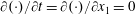 $\partial (\cdot )/\partial t=\partial (\cdot )/\partial x_{1}=0$
), thereby reducing (4.1) to
$\partial (\cdot )/\partial t=\partial (\cdot )/\partial x_{1}=0$
), thereby reducing (4.1) to
 $$\begin{eqnarray}\displaystyle \langle u_{2}\rangle _{t}{\displaystyle \frac{\partial k}{\partial x_{2}}}+\langle u_{3}\rangle _{t}{\displaystyle \frac{\partial k}{\partial x_{3}}} & {\approx} & \displaystyle -\!\left[\langle u_{2}^{\prime }u_{1}^{\prime }\rangle _{t}{\displaystyle \frac{\partial \langle u_{1}\rangle _{t}}{\partial x_{2}}}+\langle u_{3}^{\prime }u_{1}^{\prime }\rangle _{t}{\displaystyle \frac{\partial \langle u_{1}\rangle _{t}}{\partial x_{3}}}\right.\nonumber\\ \displaystyle & & \displaystyle \left.+\,\langle u_{2}^{\prime }u_{3}^{\prime }\rangle _{t}\left({\displaystyle \frac{\partial \langle u_{2}\rangle _{t}}{\partial x_{2}}}+{\displaystyle \frac{\partial \langle u_{3}\rangle _{t}}{\partial x_{2}}}\right)+(\langle (u_{2}^{\prime })^{2}\rangle _{t}-\langle (u_{3}^{\prime })^{2}\rangle _{t}){\displaystyle \frac{\partial \langle u_{2}\rangle _{t}}{\partial x_{2}}}\right]-{\it\epsilon}.\nonumber\\ \displaystyle & & \displaystyle\end{eqnarray}$$
For turbulent duct flows, Hinze (Reference Hinze1967) noted that any local non-equilibrium between production and dissipation (i.e. right-hand side of (4.2)
 $\neq 0$
) necessarily induces a local advection of
$\neq 0$
) necessarily induces a local advection of
 $\mathit{tke}$
in order to preserve conservation of energy. In the context of turbulent flows in ducts or channels, or for turbulent boundary layer flows, the above argument states that spanwise variability of
$\mathit{tke}$
in order to preserve conservation of energy. In the context of turbulent flows in ducts or channels, or for turbulent boundary layer flows, the above argument states that spanwise variability of
 $\mathit{tke}$
production close to the wall (where spatial gradients of flow quantities are largest) initializes and sustains a continual secondary flow. We can substitute the time- and streamwise-averaged LES mean flow,
$\mathit{tke}$
production close to the wall (where spatial gradients of flow quantities are largest) initializes and sustains a continual secondary flow. We can substitute the time- and streamwise-averaged LES mean flow,
 $\langle \tilde{u} _{i}\rangle _{1,t}$
, turbulent stresses,
$\langle \tilde{u} _{i}\rangle _{1,t}$
, turbulent stresses,
 $\langle \unicode[STIX]{x1D619}_{ij}\rangle _{1,t}$
, and turbulence kinetic energy,
$\langle \unicode[STIX]{x1D619}_{ij}\rangle _{1,t}$
, and turbulence kinetic energy,
 $\langle k\rangle _{1,t}$
, into (4.2) (see appendix A for discussion on retrieval of total turbulent stresses), leading to
$\langle k\rangle _{1,t}$
, into (4.2) (see appendix A for discussion on retrieval of total turbulent stresses), leading to
 $$\begin{eqnarray}\displaystyle \langle \tilde{u} _{2}\rangle _{1,t}{\displaystyle \frac{\partial \langle k\rangle _{1,t}}{\partial x_{2}}}+\langle \tilde{u} _{3}\rangle _{1,t}{\displaystyle \frac{\partial \langle k\rangle _{1,t}}{\partial x_{3}}} & {\approx} & \displaystyle -\!\left[\langle \unicode[STIX]{x1D619}_{12}\rangle _{1,t}{\displaystyle \frac{\partial \langle \tilde{u} _{1}\rangle _{1,t}}{\partial x_{2}}}+\langle \unicode[STIX]{x1D619}_{13}\rangle _{1,t}{\displaystyle \frac{\partial \langle \tilde{u} _{1}\rangle _{1,t}}{\partial x_{3}}}\right.\nonumber\\ \displaystyle & & \displaystyle \left.+\,\langle \unicode[STIX]{x1D619}_{23}\rangle _{1,t}\left({\displaystyle \frac{\partial \langle \tilde{u} _{2}\rangle _{1,t}}{\partial x_{2}}}+{\displaystyle \frac{\partial \langle \tilde{u} _{3}\rangle _{1,t}}{\partial x_{2}}}\right)\right.\nonumber\\ \displaystyle & & \displaystyle \left.+\,(\langle \unicode[STIX]{x1D619}_{22}\rangle _{1,t}-\langle \unicode[STIX]{x1D619}_{33}\rangle _{1,t}){\displaystyle \frac{\partial \langle \tilde{u} _{2}\rangle _{1,t}}{\partial x_{2}}}\right]-{\it\epsilon},\end{eqnarray}$$
where the approximation in (4.3) reflects omission of terms responsible for transport by fluctuations of pressure and velocity, and viscous stresses. From this point, we introduce the following reduced form of (4.3) for subsequent discussion,
 $$\begin{eqnarray}C_{2,k}+C_{3,k}\approx \mathscr{P}-{\it\epsilon},\end{eqnarray}$$
where
 $\mathscr{P}=\mathscr{P}_{12,k}+\mathscr{P}_{13,k}+\mathscr{P}_{23,k}+\mathscr{P}_{22,k}+\mathscr{P}_{33,k}$
represents production of
$\mathscr{P}=\mathscr{P}_{12,k}+\mathscr{P}_{13,k}+\mathscr{P}_{23,k}+\mathscr{P}_{22,k}+\mathscr{P}_{33,k}$
represents production of
 $\mathit{tke}$
associated with Reynolds-stress components denoted by subscript (i.e.
$\mathit{tke}$
associated with Reynolds-stress components denoted by subscript (i.e.
 $\mathscr{P}_{12,k}=-\langle \unicode[STIX]{x1D619}_{12}\rangle _{1,t}\partial \langle \tilde{u} _{1}\rangle _{1,t}/\partial x_{2}$
);
$\mathscr{P}_{12,k}=-\langle \unicode[STIX]{x1D619}_{12}\rangle _{1,t}\partial \langle \tilde{u} _{1}\rangle _{1,t}/\partial x_{2}$
);
 $C_{2,k}$
and
$C_{2,k}$
and
 $C_{3,k}$
denote advection of
$C_{3,k}$
denote advection of
 $\mathit{tke}$
by the secondary flow components,
$\mathit{tke}$
by the secondary flow components,
 $\langle \tilde{u} _{2}\rangle _{1,t}$
and
$\langle \tilde{u} _{2}\rangle _{1,t}$
and
 $\langle \tilde{u} _{3}\rangle _{1,t}$
, respectively. Note also that dissipation could be computed with the contraction between mean flow strain-rate tensor and subgrid-scale stress tensor,
$\langle \tilde{u} _{3}\rangle _{1,t}$
, respectively. Note also that dissipation could be computed with the contraction between mean flow strain-rate tensor and subgrid-scale stress tensor,
 ${\it\epsilon}=-{\it\tau}_{ij}\tilde{\unicode[STIX]{x1D61A}}_{ij}=-{\it\tau}_{ij}(\partial \tilde{u} _{i}/\partial x_{j}+\partial \tilde{u} _{j}/\partial x_{i})/2$
(Higgins, Parlange & Meneveau Reference Higgins, Parlange and Meneveau2004), though here we seek simply to identify regions of ‘maximum’ production of turbulence in order to infer mean flow orientations, since it is the local imbalance between production and dissipation (not the magnitude of the imbalance) that induces the secondary flow direction.
${\it\epsilon}=-{\it\tau}_{ij}\tilde{\unicode[STIX]{x1D61A}}_{ij}=-{\it\tau}_{ij}(\partial \tilde{u} _{i}/\partial x_{j}+\partial \tilde{u} _{j}/\partial x_{i})/2$
(Higgins, Parlange & Meneveau Reference Higgins, Parlange and Meneveau2004), though here we seek simply to identify regions of ‘maximum’ production of turbulence in order to infer mean flow orientations, since it is the local imbalance between production and dissipation (not the magnitude of the imbalance) that induces the secondary flow direction.


Figure 6. Contours of
 $k$
production terms in (4.3) and (4.4) from experimental results of flow over figure 1(a) complex roughness (Barros & Christensen Reference Barros and Christensen2014) where panels correspond to: (a)
$k$
production terms in (4.3) and (4.4) from experimental results of flow over figure 1(a) complex roughness (Barros & Christensen Reference Barros and Christensen2014) where panels correspond to: (a)
 $\mathscr{P}_{12,k}$
; (b)
$\mathscr{P}_{12,k}$
; (b)
 $\mathscr{P}_{23,k}$
; (c)
$\mathscr{P}_{23,k}$
; (c)
 $\mathscr{P}_{13,k}$
; (d)
$\mathscr{P}_{13,k}$
; (d)
 $\mathscr{P}_{22,k}$
; and (e)
$\mathscr{P}_{22,k}$
; and (e)
 $\mathscr{P}_{33,k}$
.
$\mathscr{P}_{33,k}$
.
Figures 5 and 6 show the individual production terms that compose
 $\mathscr{P}$
in (4.4) from the LES and experimental results, respectively. Figure 5(a,c,e,g,i) shows results for
$\mathscr{P}$
in (4.4) from the LES and experimental results, respectively. Figure 5(a,c,e,g,i) shows results for
 ${\it\lambda}=2$
(‘smallest’ value) and figure 5(b,d, f,h, j) those for
${\it\lambda}=2$
(‘smallest’ value) and figure 5(b,d, f,h, j) those for
 ${\it\lambda}=900$
(‘largest’ value). It is apparent for both the LES and experimental results that
${\it\lambda}=900$
(‘largest’ value). It is apparent for both the LES and experimental results that
 $\mathit{tke}$
production associated with the streamwise-wall normal component,
$\mathit{tke}$
production associated with the streamwise-wall normal component,
 $\mathscr{P}_{13,k}$
, greatly exceeds production via other terms. Moreover, and more importantly, we note that the elevation corresponding to
$\mathscr{P}_{13,k}$
, greatly exceeds production via other terms. Moreover, and more importantly, we note that the elevation corresponding to
 $\text{max}(\mathscr{P}_{13,k})$
varies in
$\text{max}(\mathscr{P}_{13,k})$
varies in
 $x_{2}$
. For the LES cases, the
$x_{2}$
. For the LES cases, the
 $\text{max}(\mathscr{P}_{13,k})$
value is clearly correlated with the topography, wherein the peak value occurs above the
$\text{max}(\mathscr{P}_{13,k})$
value is clearly correlated with the topography, wherein the peak value occurs above the
 $z_{0,H}$
strip, close to the wall. This is particularly clear for
$z_{0,H}$
strip, close to the wall. This is particularly clear for
 ${\it\lambda}=900$
(figure 5
f). For the experiments, the position of
${\it\lambda}=900$
(figure 5
f). For the experiments, the position of
 $\text{max}(\mathscr{P}_{13,k})$
is not as readily visible since experimental measurements of turbulence statistics are not available for
$\text{max}(\mathscr{P}_{13,k})$
is not as readily visible since experimental measurements of turbulence statistics are not available for
 $x_{3}/{\it\delta}\lesssim 0.07$
(figure 6
c). However, within the LMPs (
$x_{3}/{\it\delta}\lesssim 0.07$
(figure 6
c). However, within the LMPs (
 $x_{2}/{\it\delta}\approx 1$
, 0.2,
$x_{2}/{\it\delta}\approx 1$
, 0.2,
 $-0.6$
) there is clear elevated
$-0.6$
) there is clear elevated
 $\mathscr{P}_{13,k}$
far from the wall above the ‘low’ roughness (topographic depressions). It is also apparent that relative peaks in
$\mathscr{P}_{13,k}$
far from the wall above the ‘low’ roughness (topographic depressions). It is also apparent that relative peaks in
 $\mathscr{P}_{12,k}$
for the experimental data occur at positions adjacent to topographic peaks. (For example, consider the topographic peak at
$\mathscr{P}_{12,k}$
for the experimental data occur at positions adjacent to topographic peaks. (For example, consider the topographic peak at
 $x_{2}/{\it\delta}\approx -1$
and the adjacent
$x_{2}/{\it\delta}\approx -1$
and the adjacent
 $\mathscr{P}_{12,k}$
values at
$\mathscr{P}_{12,k}$
values at
 $x_{2}/{\it\delta}\approx -1.2$
and
$x_{2}/{\it\delta}\approx -1.2$
and
 $-0.8$
; this production is due to the presence of vertical shearing layers between adjacent HMPs/LMPs and clearly illustrates linkages between the complex roughness and processes in the above turbulence (Vermaas et al.
Reference Vermaas, Uijttewall and Hoitink2011; Willingham et al.
Reference Willingham, Anderson, Christensen and Barros2013).) Since
$-0.8$
; this production is due to the presence of vertical shearing layers between adjacent HMPs/LMPs and clearly illustrates linkages between the complex roughness and processes in the above turbulence (Vermaas et al.
Reference Vermaas, Uijttewall and Hoitink2011; Willingham et al.
Reference Willingham, Anderson, Christensen and Barros2013).) Since
 $\mathscr{P}_{13,k}$
effectively dominates the
$\mathscr{P}_{13,k}$
effectively dominates the
 $\mathit{tke}$
production (production and destruction associated with other stresses and mean flow gradients are relatively mild), we can state that
$\mathit{tke}$
production (production and destruction associated with other stresses and mean flow gradients are relatively mild), we can state that
 $\mathscr{P}\approx \mathscr{P}_{13,k}$
. Moreover, recall that production and dissipation of tke (in the LES context) are computed as the product of mean flow gradients and the total (Reynolds) stress,
$\mathscr{P}\approx \mathscr{P}_{13,k}$
. Moreover, recall that production and dissipation of tke (in the LES context) are computed as the product of mean flow gradients and the total (Reynolds) stress,
 $\unicode[STIX]{x1D619}_{ij}$
, and subgrid-scale stress,
$\unicode[STIX]{x1D619}_{ij}$
, and subgrid-scale stress,
 ${\it\tau}_{ij}$
, respectively (Higgins et al.
Reference Higgins, Parlange and Meneveau2004). Since, by definition,
${\it\tau}_{ij}$
, respectively (Higgins et al.
Reference Higgins, Parlange and Meneveau2004). Since, by definition,
 ${\it\tau}_{ij}\leqslant \unicode[STIX]{x1D619}_{ij}$
(and, in fact, far from the wall,
${\it\tau}_{ij}\leqslant \unicode[STIX]{x1D619}_{ij}$
(and, in fact, far from the wall,
 $\unicode[STIX]{x1D619}_{13}/{\it\tau}_{13}\sim \mathit{O}(10)$
(Porté-Agel, Meneveau & Parlange Reference Porté-Agel, Meneveau and Parlange2000; Bou-Zeid et al.
Reference Bou-Zeid, Meneveau and Parlange2005; Anderson & Meneveau Reference Anderson and Meneveau2011)), it is clear that production should exceed dissipation. Owing to the heterogeneity of the topography (especially in the spanwise direction), there must therefore be spanwise heterogeneity in the production–dissipation balance,
$\unicode[STIX]{x1D619}_{13}/{\it\tau}_{13}\sim \mathit{O}(10)$
(Porté-Agel, Meneveau & Parlange Reference Porté-Agel, Meneveau and Parlange2000; Bou-Zeid et al.
Reference Bou-Zeid, Meneveau and Parlange2005; Anderson & Meneveau Reference Anderson and Meneveau2011)), it is clear that production should exceed dissipation. Owing to the heterogeneity of the topography (especially in the spanwise direction), there must therefore be spanwise heterogeneity in the production–dissipation balance,
 $\mathscr{P}\neq {\it\epsilon}$
. The greatest excess of production over dissipation must be in the fluid immediately above the
$\mathscr{P}\neq {\it\epsilon}$
. The greatest excess of production over dissipation must be in the fluid immediately above the
 $z_{0,H}$
strip (that is, the most ‘turbulence-rich’ fluid, in Hinze’s parlance (Hinze Reference Hinze1973)). Similarly, consultation of figure 6(c) and the solid black profile beneath – representative height of complex roughness and therefore proxy for imposed aerodynamic stress – shows that elevated
$z_{0,H}$
strip (that is, the most ‘turbulence-rich’ fluid, in Hinze’s parlance (Hinze Reference Hinze1973)). Similarly, consultation of figure 6(c) and the solid black profile beneath – representative height of complex roughness and therefore proxy for imposed aerodynamic stress – shows that elevated
 $\mathscr{P}_{13,k}$
is clearly present above the high-drag (relatively elevated roughness) positions.
$\mathscr{P}_{13,k}$
is clearly present above the high-drag (relatively elevated roughness) positions.
Figure 7 shows the corresponding
 $\mathit{tke}$
advection terms in (4.4) for the LES (figure 7
a,b) and experimental results (figure 7
c). It is clear that the largest
$\mathit{tke}$
advection terms in (4.4) for the LES (figure 7
a,b) and experimental results (figure 7
c). It is clear that the largest
 $\mathit{tke}$
advection occurs close to the wall, owing to the strong secondary flow velocity components. We see that
$\mathit{tke}$
advection occurs close to the wall, owing to the strong secondary flow velocity components. We see that
 $C_{2,k}+C_{3,k}>0$
within the HMP, pointing to production exceeding dissipation in the HMP, or
$C_{2,k}+C_{3,k}>0$
within the HMP, pointing to production exceeding dissipation in the HMP, or
 $\mathscr{P}-{\it\epsilon}>0$
. We have determined that, within the HMP,
$\mathscr{P}-{\it\epsilon}>0$
. We have determined that, within the HMP,
 $C_{2,k}\approx 0$
. Therefore,
$C_{2,k}\approx 0$
. Therefore,
 $C_{3,k}\approx \mathscr{P}-{\it\epsilon}$
within the HMP. However, we also showed in the
$C_{3,k}\approx \mathscr{P}-{\it\epsilon}$
within the HMP. However, we also showed in the
 $\mathit{tke}$
contour (figure 4
m,n) that vertical (wall normal) gradients of
$\mathit{tke}$
contour (figure 4
m,n) that vertical (wall normal) gradients of
 $\mathit{tke}$
are negative at all spanwise positions. Thus, if
$\mathit{tke}$
are negative at all spanwise positions. Thus, if
 $\partial k/\partial x_{3}<0$
but
$\partial k/\partial x_{3}<0$
but
 $C_{3,k}\approx \mathscr{P}-{\it\epsilon}>0$
within the HMP, then the mean vertical velocity must be negative,
$C_{3,k}\approx \mathscr{P}-{\it\epsilon}>0$
within the HMP, then the mean vertical velocity must be negative,
 $\langle \tilde{u} _{3}\rangle _{1,t}<0$
, in order to realize a balance in the
$\langle \tilde{u} _{3}\rangle _{1,t}<0$
, in order to realize a balance in the
 $\mathit{tke}$
transport equation: on figure 7, we have included solid black contours of
$\mathit{tke}$
transport equation: on figure 7, we have included solid black contours of
 $\langle \tilde{u} _{3}\rangle _{1,t}\leqslant 0$
and these largely embody the HMP.
$\langle \tilde{u} _{3}\rangle _{1,t}\leqslant 0$
and these largely embody the HMP.

Figure 7. Continuous colour contours illustrate advective terms,
 $C_{2,k}+C_{3,k}$
, in (4.4) associated with transport of
$C_{2,k}+C_{3,k}$
, in (4.4) associated with transport of
 $k$
by mean secondary flow for: (a)
$k$
by mean secondary flow for: (a)
 ${\it\lambda}=2$
, (b)
${\it\lambda}=2$
, (b)
 ${\it\lambda}=900$
and (c) experimental results for flow over complex roughness (Barros & Christensen Reference Barros and Christensen2014). Solid black contours are mean vertical velocity less than zero,
${\it\lambda}=900$
and (c) experimental results for flow over complex roughness (Barros & Christensen Reference Barros and Christensen2014). Solid black contours are mean vertical velocity less than zero,
 $\langle \tilde{u} _{3}\rangle _{1,t}\leqslant 0$
.
$\langle \tilde{u} _{3}\rangle _{1,t}\leqslant 0$
.
Since the dominant production term is
 $\mathscr{P}_{13}$
, this effectively sets the secondary flow in motion and sustains it continually. In order to preserve mean flow continuity,
$\mathscr{P}_{13}$
, this effectively sets the secondary flow in motion and sustains it continually. In order to preserve mean flow continuity,
 $\partial \langle \tilde{u} _{2}\rangle _{1,t}/\partial x_{2}+\partial \langle \tilde{u} _{3}\rangle _{1,t}/\partial x_{3}=0$
(following enforcement of the streamwise homogeneity condition), the vigorous
$\partial \langle \tilde{u} _{2}\rangle _{1,t}/\partial x_{2}+\partial \langle \tilde{u} _{3}\rangle _{1,t}/\partial x_{3}=0$
(following enforcement of the streamwise homogeneity condition), the vigorous
 $\langle \tilde{u} _{3}\rangle _{1,t}\leqslant 0$
within the HMP must be balanced by a lateral outflow (spanwise velocity) close to the wall. The result of this is evident in figure 7, where we see
$\langle \tilde{u} _{3}\rangle _{1,t}\leqslant 0$
within the HMP must be balanced by a lateral outflow (spanwise velocity) close to the wall. The result of this is evident in figure 7, where we see
 $C_{2,k}+C_{3,k}<0$
for
$C_{2,k}+C_{3,k}<0$
for
 $x_{3}/{\it\delta}\lesssim 0.25$
on either side of the HMP. We have determined that, above
$x_{3}/{\it\delta}\lesssim 0.25$
on either side of the HMP. We have determined that, above
 $z_{0,L}$
(or the black profile that is an indicator of imposed drag by the complex roughness),
$z_{0,L}$
(or the black profile that is an indicator of imposed drag by the complex roughness),
 $C_{3,k}\approx 0$
, and therefore advection is exclusively via the spanwise component of the secondary flow. Since
$C_{3,k}\approx 0$
, and therefore advection is exclusively via the spanwise component of the secondary flow. Since
 $\mathit{tke}$
exhibits a spanwise heterogeneity (figure 4
m,n) in which it is higher within the HMP base, close to the wall, lateral
$\mathit{tke}$
exhibits a spanwise heterogeneity (figure 4
m,n) in which it is higher within the HMP base, close to the wall, lateral
 $\mathit{tke}$
gradients are negative (in the high- to low-drag direction) and
$\mathit{tke}$
gradients are negative (in the high- to low-drag direction) and
 $C_{2,k}$
must be negative. Again, we stress that the objective here is simply to identify driving mechanisms responsible for setting the secondary flow in motion and therefore subtracting the actual dissipation from LES and rigorously balancing equation (4.4) is not essential to the present analysis. This conceptual approach to understanding these turbulent secondary flows has been studied also by the open-channel flow community (see, for example, the recent study by Vermaas et al. (Reference Vermaas, Uijttewall and Hoitink2011)). The turbulent duct flow literature tended to focus more on the mean streamwise vorticity transport equation when identifying underlying secondary flow production mechanisms (Hoagland Reference Hoagland1960; Brundrett & Baines Reference Brundrett and Baines1964; Bradshaw Reference Bradshaw1987; Madabhushi & Vanka Reference Madabhushi and Vanka1991); in the following, we demonstrate application of this approach for the present flow configurations.
$C_{2,k}$
must be negative. Again, we stress that the objective here is simply to identify driving mechanisms responsible for setting the secondary flow in motion and therefore subtracting the actual dissipation from LES and rigorously balancing equation (4.4) is not essential to the present analysis. This conceptual approach to understanding these turbulent secondary flows has been studied also by the open-channel flow community (see, for example, the recent study by Vermaas et al. (Reference Vermaas, Uijttewall and Hoitink2011)). The turbulent duct flow literature tended to focus more on the mean streamwise vorticity transport equation when identifying underlying secondary flow production mechanisms (Hoagland Reference Hoagland1960; Brundrett & Baines Reference Brundrett and Baines1964; Bradshaw Reference Bradshaw1987; Madabhushi & Vanka Reference Madabhushi and Vanka1991); in the following, we demonstrate application of this approach for the present flow configurations.
5. Mean vorticity
Figure 8 shows spanwise-vertical contours of components of the vorticity vector for the controlled LES cases of
 ${\it\lambda}=2$
and 100, as outlined in the figure caption, while figure 9 presents the same from the experimental results of flow over the complex roughness. The presence of mean streamwise vorticity in the form of
${\it\lambda}=2$
and 100, as outlined in the figure caption, while figure 9 presents the same from the experimental results of flow over the complex roughness. The presence of mean streamwise vorticity in the form of
 ${\it\delta}$
-scale roll cells is evident for both
${\it\delta}$
-scale roll cells is evident for both
 ${\it\lambda}$
values considered (figure 8
a,b) and in the experimental results (figure 9
a). This has been to some extent outlined also in figure 2(c,d) and the accompanying discussion, where swirl strength with the sign of
${\it\lambda}$
values considered (figure 8
a,b) and in the experimental results (figure 9
a). This has been to some extent outlined also in figure 2(c,d) and the accompanying discussion, where swirl strength with the sign of
 $\langle \tilde{{\it\omega}}_{1}\rangle _{1,t}$
was used to demonstrate the presence of rotating cells. The large values of
$\langle \tilde{{\it\omega}}_{1}\rangle _{1,t}$
was used to demonstrate the presence of rotating cells. The large values of
 $\langle \tilde{{\it\omega}}_{1}\rangle _{1,t}$
close to the surface are due to the strong lateral outflow at the base of the HMPs (as was discussed in § 4) and associated large vertical gradient of
$\langle \tilde{{\it\omega}}_{1}\rangle _{1,t}$
close to the surface are due to the strong lateral outflow at the base of the HMPs (as was discussed in § 4) and associated large vertical gradient of
 $\langle \tilde{u} _{2}\rangle _{1,t}$
in this region. We see essentially the same spatial pattern of
$\langle \tilde{u} _{2}\rangle _{1,t}$
in this region. We see essentially the same spatial pattern of
 $\langle \tilde{{\it\omega}}_{1}\rangle _{1,t}$
for
$\langle \tilde{{\it\omega}}_{1}\rangle _{1,t}$
for
 ${\it\lambda}$
changing by roughly two orders of magnitude as well as in the presence of significant topographical complexity (figure 9). Figure 8(c,d) as well as figure 9(b) show mean spanwise vorticity for the LES and experimental cases, respectively, which is equivalent to the wall-normal gradient of mean streamwise velocity. From these figures, we emphasize that the largest
${\it\lambda}$
changing by roughly two orders of magnitude as well as in the presence of significant topographical complexity (figure 9). Figure 8(c,d) as well as figure 9(b) show mean spanwise vorticity for the LES and experimental cases, respectively, which is equivalent to the wall-normal gradient of mean streamwise velocity. From these figures, we emphasize that the largest
 $\langle \tilde{{\it\omega}}_{2}\rangle _{1,t}=\partial \langle \tilde{u} _{1}\rangle _{1,t}/\partial x_{3}$
occurs above
$\langle \tilde{{\it\omega}}_{2}\rangle _{1,t}=\partial \langle \tilde{u} _{1}\rangle _{1,t}/\partial x_{3}$
occurs above
 $z_{0,H}$
, at the base of the HMP (especially clear for
$z_{0,H}$
, at the base of the HMP (especially clear for
 ${\it\lambda}=100$
, figure 8
d). This figure then is consistent with previous comments on the spanwise variation of imposed wall stress (figure 3 and accompanying text) in the context of sustaining the secondary flow, since the elevated
${\it\lambda}=100$
, figure 8
d). This figure then is consistent with previous comments on the spanwise variation of imposed wall stress (figure 3 and accompanying text) in the context of sustaining the secondary flow, since the elevated
 $\partial \langle \tilde{u} _{1}\rangle _{1,t}/\partial x_{3}$
facilitates enhanced downward momentum fluxes, which are ultimately absorbed by the roughness.
$\partial \langle \tilde{u} _{1}\rangle _{1,t}/\partial x_{3}$
facilitates enhanced downward momentum fluxes, which are ultimately absorbed by the roughness.

Figure 8. Contours of mean vorticity,
 $\langle \tilde{{\bf\omega}}\rangle _{1,t}=\{\langle \tilde{{\it\omega}}_{1}\rangle _{1,t},\langle \tilde{{\it\omega}}_{2}\rangle _{1,t},\langle \tilde{{\it\omega}}_{3}\rangle _{1,t}\}$
for (a,c,e)
$\langle \tilde{{\bf\omega}}\rangle _{1,t}=\{\langle \tilde{{\it\omega}}_{1}\rangle _{1,t},\langle \tilde{{\it\omega}}_{2}\rangle _{1,t},\langle \tilde{{\it\omega}}_{3}\rangle _{1,t}\}$
for (a,c,e)
 ${\it\lambda}=2$
and (b,d, f)
${\it\lambda}=2$
and (b,d, f)
 ${\it\lambda}=100$
: (a,b)
${\it\lambda}=100$
: (a,b)
 $\langle \tilde{{\it\omega}}_{1}\rangle _{1,t}=\partial \langle \tilde{u} _{3}\rangle _{1,t}/\partial x_{2}-\partial \langle \tilde{u} _{2}\rangle _{1,t}/\partial x_{3}$
; (c,d)
$\langle \tilde{{\it\omega}}_{1}\rangle _{1,t}=\partial \langle \tilde{u} _{3}\rangle _{1,t}/\partial x_{2}-\partial \langle \tilde{u} _{2}\rangle _{1,t}/\partial x_{3}$
; (c,d)
 $\langle \tilde{{\it\omega}}_{2}\rangle _{1,t}=\partial \langle \tilde{u} _{1}\rangle _{1,t}/\partial x_{3}$
; and (e, f)
$\langle \tilde{{\it\omega}}_{2}\rangle _{1,t}=\partial \langle \tilde{u} _{1}\rangle _{1,t}/\partial x_{3}$
; and (e, f)
 $\langle \tilde{{\it\omega}}_{3}\rangle _{1,t}=-\partial \langle \tilde{u} _{1}\rangle _{1,t}/\partial x_{2}$
.
$\langle \tilde{{\it\omega}}_{3}\rangle _{1,t}=-\partial \langle \tilde{u} _{1}\rangle _{1,t}/\partial x_{2}$
.

Figure 9. Contours of mean vorticity from experimental results of flow over complex roughness (Barros & Christensen Reference Barros and Christensen2014): (a)
 $\langle \tilde{{\it\omega}}_{1}\rangle _{1,t}$
; (b)
$\langle \tilde{{\it\omega}}_{1}\rangle _{1,t}$
; (b)
 $\langle \tilde{{\it\omega}}_{2}\rangle _{1,t}$
; and (c)
$\langle \tilde{{\it\omega}}_{2}\rangle _{1,t}$
; and (c)
 $\langle \tilde{{\it\omega}}_{3}\rangle _{1,t}$
.
$\langle \tilde{{\it\omega}}_{3}\rangle _{1,t}$
.
Similarly, figure 9(b) shows elevated
 $\langle \tilde{{\it\omega}}_{2}\rangle _{1,t}$
at the base of HMPs, above regions of relatively higher imposed drag. Finally, figures 8(e, f) and 9(c) show vertical vorticity,
$\langle \tilde{{\it\omega}}_{2}\rangle _{1,t}$
at the base of HMPs, above regions of relatively higher imposed drag. Finally, figures 8(e, f) and 9(c) show vertical vorticity,
 $\langle \tilde{{\it\omega}}_{3}\rangle _{1,t}$
, which under the SSH condition illustrates the spanwise gradient of mean streamwise velocity. For the figure 1(b) roughness, Willingham et al. (Reference Willingham, Anderson, Christensen and Barros2013) have argued that the presence of the spanwise roughness heterogeneity and resultant wall stress distribution (figure 3) serve to introduce a vertically inclined mixing layer in the flow, which facilitates a lateral momentum exchange via
$\langle \tilde{{\it\omega}}_{3}\rangle _{1,t}$
, which under the SSH condition illustrates the spanwise gradient of mean streamwise velocity. For the figure 1(b) roughness, Willingham et al. (Reference Willingham, Anderson, Christensen and Barros2013) have argued that the presence of the spanwise roughness heterogeneity and resultant wall stress distribution (figure 3) serve to introduce a vertically inclined mixing layer in the flow, which facilitates a lateral momentum exchange via
 $\unicode[STIX]{x1D619}_{12}$
(figure 4
k) in a region close to the wall. This was consistent with concepts already developed for open channel flows over adjacent ‘regions’ of differing roughness developed by the hydraulic engineering community; for example see Wang & Cheng (Reference Wang and Cheng2005) and Vermaas et al. (Reference Vermaas, Uijttewall and Hoitink2011). Thus, figure 8(e, f) shows the spanwise mean flow gradient inherent to this lateral momentum exchange and, indeed, this quantity exhibits extreme values (positive and negative) in a small region precisely above the roughness heterogeneity. Similar patterns are readily apparent in the experimental results for flow over complex roughness (figure 9
c). Further, we emphasize consistency in the polarity of
$\unicode[STIX]{x1D619}_{12}$
(figure 4
k) in a region close to the wall. This was consistent with concepts already developed for open channel flows over adjacent ‘regions’ of differing roughness developed by the hydraulic engineering community; for example see Wang & Cheng (Reference Wang and Cheng2005) and Vermaas et al. (Reference Vermaas, Uijttewall and Hoitink2011). Thus, figure 8(e, f) shows the spanwise mean flow gradient inherent to this lateral momentum exchange and, indeed, this quantity exhibits extreme values (positive and negative) in a small region precisely above the roughness heterogeneity. Similar patterns are readily apparent in the experimental results for flow over complex roughness (figure 9
c). Further, we emphasize consistency in the polarity of
 $\langle \tilde{{\it\omega}}_{3}\rangle _{1,t}$
in the zone immediately above the roughness heterogeneity (
$\langle \tilde{{\it\omega}}_{3}\rangle _{1,t}$
in the zone immediately above the roughness heterogeneity (
 $x_{3}/{\it\delta}\lesssim 0.1$
): positive (negative) on the ‘left’ (‘right’) side of the
$x_{3}/{\it\delta}\lesssim 0.1$
): positive (negative) on the ‘left’ (‘right’) side of the
 $z_{0,H}$
strips, owing to spanwise decrease (increase) of
$z_{0,H}$
strips, owing to spanwise decrease (increase) of
 $\langle \tilde{u} _{1}\rangle _{1,t}$
in response to increasing (decreasing) wall stress imposed by the
$\langle \tilde{u} _{1}\rangle _{1,t}$
in response to increasing (decreasing) wall stress imposed by the
 $z_{0,H}~(z_{0,L})$
strip. Above this region (
$z_{0,H}~(z_{0,L})$
strip. Above this region (
 $x_{3}/{\it\delta}>0.1$
), the polarity of
$x_{3}/{\it\delta}>0.1$
), the polarity of
 $\langle \tilde{{\it\omega}}_{3}\rangle _{1,t}$
reverses due to the adjacent HMPs/LMPs. Similarly, consultation of the 2(b) shows positioning of the HMPs with respect to the complex roughness, and one may contrast this against the figure 9(c) contours of
$\langle \tilde{{\it\omega}}_{3}\rangle _{1,t}$
reverses due to the adjacent HMPs/LMPs. Similarly, consultation of the 2(b) shows positioning of the HMPs with respect to the complex roughness, and one may contrast this against the figure 9(c) contours of
 $\langle \tilde{{\it\omega}}_{3}\rangle _{1,t}$
. Qualitative agreement with underlying processes for the LES topographies is strong.
$\langle \tilde{{\it\omega}}_{3}\rangle _{1,t}$
. Qualitative agreement with underlying processes for the LES topographies is strong.
The mean streamwise vorticity,
 $\langle \tilde{{\it\omega}}_{1}\rangle _{t}$
, transport equation (with Reynolds stresses substituted from LES,
$\langle \tilde{{\it\omega}}_{1}\rangle _{t}$
, transport equation (with Reynolds stresses substituted from LES,
 $\unicode[STIX]{x1D619}_{ij}$
) is
$\unicode[STIX]{x1D619}_{ij}$
) is
 $$\begin{eqnarray}\displaystyle & & \displaystyle \langle \tilde{u} _{1}\rangle _{t}{\displaystyle \frac{\partial \langle \tilde{{\it\omega}}_{1}\rangle _{t}}{\partial x_{1}}}+\langle \tilde{u} _{2}\rangle _{t}{\displaystyle \frac{\partial \langle \tilde{{\it\omega}}_{1}\rangle _{t}}{\partial x_{2}}}+\langle \tilde{u} _{3}\rangle _{t}{\displaystyle \frac{\partial \langle \tilde{{\it\omega}}_{1}\rangle _{t}}{\partial x_{3}}}\nonumber\\ \displaystyle & & \displaystyle \quad ={\it\nu}\left({\displaystyle \frac{\partial ^{2}\langle \tilde{{\it\omega}}_{1}\rangle _{t}}{\partial {x_{1}}^{2}}}+{\displaystyle \frac{\partial ^{2}\langle \tilde{{\it\omega}}_{1}\rangle _{t}}{\partial {x_{2}}^{2}}}+{\displaystyle \frac{\partial ^{2}\langle \tilde{{\it\omega}}_{1}\rangle _{t}}{\partial {x_{3}}^{2}}}\right)+\langle \tilde{{\it\omega}}_{1}\rangle _{t}{\displaystyle \frac{\partial \langle \tilde{u} _{1}\rangle _{t}}{\partial x_{1}}}+\langle \tilde{{\it\omega}}_{2}\rangle _{t}{\displaystyle \frac{\partial \langle \tilde{u} _{1}\rangle _{t}}{\partial x_{2}}}\nonumber\\ \displaystyle & & \displaystyle \qquad +\,\langle \tilde{{\it\omega}}_{3}\rangle _{t}{\displaystyle \frac{\partial \langle \tilde{u} _{1}\rangle _{t}}{\partial x_{3}}}+\,{\displaystyle \frac{\partial ^{2}}{\partial x_{2}\partial x_{3}}}\left[\langle \unicode[STIX]{x1D619}_{22}\rangle _{t}-\langle \unicode[STIX]{x1D619}_{33}\rangle _{t}\right]-{\displaystyle \frac{\partial ^{2}\langle \unicode[STIX]{x1D619}_{23}\rangle _{t}}{\partial x_{2}^{2}}}+{\displaystyle \frac{\partial ^{2}\langle \unicode[STIX]{x1D619}_{23}\rangle _{t}}{\partial x_{3}^{2}}}\nonumber\\ \displaystyle & & \displaystyle \qquad +\,{\displaystyle \frac{\partial }{\partial x_{1}}}\left({\displaystyle \frac{\partial \langle \unicode[STIX]{x1D619}_{12}\rangle _{t}}{\partial x_{3}}}-{\displaystyle \frac{\partial \langle \unicode[STIX]{x1D619}_{13}\rangle _{t}}{\partial x_{2}}}\right),\end{eqnarray}$$
where the left-hand side terms represent mean flow advection of
 $\langle \tilde{{\it\omega}}_{1}\rangle _{t}$
, the first right-hand side term represents dissipation of
$\langle \tilde{{\it\omega}}_{1}\rangle _{t}$
, the first right-hand side term represents dissipation of
 $\langle \tilde{{\it\omega}}_{1}\rangle _{t}$
, the
$\langle \tilde{{\it\omega}}_{1}\rangle _{t}$
, the
 $\langle \tilde{{\bf\omega}}\rangle \boldsymbol{\cdot }\boldsymbol{{\rm\nabla}}\langle \tilde{\boldsymbol{u}}\rangle _{t}$
terms represent vortex tilting and stretching, and the final second-order derivatives are
$\langle \tilde{{\bf\omega}}\rangle \boldsymbol{\cdot }\boldsymbol{{\rm\nabla}}\langle \tilde{\boldsymbol{u}}\rangle _{t}$
terms represent vortex tilting and stretching, and the final second-order derivatives are
 $\langle \tilde{{\it\omega}}_{1}\rangle _{t}$
production by spatial gradients in the Reynolds stresses. Prandtl’s secondary flows may be of the first or second kind, where the first kind is attributed to vortex stretching and tilting while the second is attributed to anisotropy of the Reynolds stresses (Perkins Reference Perkins1970; Bradshaw Reference Bradshaw1987; Madabhushi & Vanka Reference Madabhushi and Vanka1991). Equation (5.1) can be reduced considerably by application of the streamwise homogeneity condition,
$\langle \tilde{{\it\omega}}_{1}\rangle _{t}$
production by spatial gradients in the Reynolds stresses. Prandtl’s secondary flows may be of the first or second kind, where the first kind is attributed to vortex stretching and tilting while the second is attributed to anisotropy of the Reynolds stresses (Perkins Reference Perkins1970; Bradshaw Reference Bradshaw1987; Madabhushi & Vanka Reference Madabhushi and Vanka1991). Equation (5.1) can be reduced considerably by application of the streamwise homogeneity condition,
 $\partial (\cdot )/\partial x_{1}=0$
, and neglecting viscous diffusion terms; in the absence of streamwise heterogeneity, the components of mean vorticity in the spanwise and vertical directions are
$\partial (\cdot )/\partial x_{1}=0$
, and neglecting viscous diffusion terms; in the absence of streamwise heterogeneity, the components of mean vorticity in the spanwise and vertical directions are
 $\langle \tilde{{\it\omega}}_{2}\rangle _{1,t}=\partial \langle \tilde{u} _{1}\rangle _{1,t}/\partial x_{3}$
and
$\langle \tilde{{\it\omega}}_{2}\rangle _{1,t}=\partial \langle \tilde{u} _{1}\rangle _{1,t}/\partial x_{3}$
and
 $\langle \tilde{{\it\omega}}_{3}\rangle _{t}=-\partial \langle \tilde{u} _{1}\rangle _{1,t}/\partial x_{2}$
, respectively. Thus, we immediately observe that mean flow vortex stretching is by definition zero, and the current flow is therefore Prandtl’s secondary flow of the second kind (see also spanwise-vertical distributions of the Reynolds-stress tensor components in figure 4). Equation (5.1) then reduces to
$\langle \tilde{{\it\omega}}_{3}\rangle _{t}=-\partial \langle \tilde{u} _{1}\rangle _{1,t}/\partial x_{2}$
, respectively. Thus, we immediately observe that mean flow vortex stretching is by definition zero, and the current flow is therefore Prandtl’s secondary flow of the second kind (see also spanwise-vertical distributions of the Reynolds-stress tensor components in figure 4). Equation (5.1) then reduces to
 $$\begin{eqnarray}\langle \tilde{u} _{2}\rangle _{1,t}{\displaystyle \frac{\partial \langle \tilde{{\it\omega}}_{1}\rangle _{1,t}}{\partial x_{2}}}+\langle \tilde{u} _{3}\rangle _{1,t}{\displaystyle \frac{\partial \langle \tilde{{\it\omega}}_{1}\rangle _{1,t}}{\partial x_{3}}}\approx {\displaystyle \frac{\partial ^{2}}{\partial x_{2}\partial x_{3}}}[\langle \unicode[STIX]{x1D619}_{22}\rangle _{1,t}-\langle \unicode[STIX]{x1D619}_{33}\rangle _{1,t}]-{\displaystyle \frac{\partial ^{2}\langle \unicode[STIX]{x1D619}_{23}\rangle _{1,t}}{\partial x_{2}^{2}}}+{\displaystyle \frac{\partial ^{2}\langle \unicode[STIX]{x1D619}_{23}\rangle _{1,t}}{\partial x_{3}^{2}}}.\end{eqnarray}$$
Equation (5.2) is a statement that mean streamwise vorticity is advected throughout the domain by the spanwise-vertical mean secondary flow, and this occurs via production associated with spatial gradients of components of the Reynolds stresses. For convenience only, we rewrite (5.2) as
 $$\begin{eqnarray}C_{2,\tilde{{\it\omega}}_{1}}+C_{3,\tilde{{\it\omega}}_{1}}\approx P_{N,\tilde{{\it\omega}}_{1}}+P_{\mathit{S},\tilde{{\it\omega}}_{1}},\end{eqnarray}$$
where
 $C_{2,\tilde{{\it\omega}}_{1}}$
and
$C_{2,\tilde{{\it\omega}}_{1}}$
and
 $C_{3,\tilde{{\it\omega}}_{1}}$
represent
$C_{3,\tilde{{\it\omega}}_{1}}$
represent
 $\langle \tilde{{\it\omega}}_{1}\rangle _{1,t}$
advection by the mean spanwise and vertical secondary flow components, respectively,
$\langle \tilde{{\it\omega}}_{1}\rangle _{1,t}$
advection by the mean spanwise and vertical secondary flow components, respectively,
 $P_{N,\tilde{{\it\omega}}_{1}}$
represents production due to the Reynolds normal stresses (
$P_{N,\tilde{{\it\omega}}_{1}}$
represents production due to the Reynolds normal stresses (
 $\unicode[STIX]{x1D619}_{22}$
and
$\unicode[STIX]{x1D619}_{22}$
and
 $\unicode[STIX]{x1D619}_{33}$
), and
$\unicode[STIX]{x1D619}_{33}$
), and
 $P_{N,\tilde{{\it\omega}}_{1}}$
represents production by Reynolds shear stress,
$P_{N,\tilde{{\it\omega}}_{1}}$
represents production by Reynolds shear stress,
 $\unicode[STIX]{x1D619}_{23}$
.
$\unicode[STIX]{x1D619}_{23}$
.
Figure 10 shows contours of terms responsible for production and advection of
 $\langle \tilde{{\it\omega}}_{1}\rangle _{1,t}$
in (5.3) for two
$\langle \tilde{{\it\omega}}_{1}\rangle _{1,t}$
in (5.3) for two
 ${\it\lambda}$
values that differ by roughly two orders of magnitude (
${\it\lambda}$
values that differ by roughly two orders of magnitude (
 ${\it\lambda}=25$
and
${\it\lambda}=25$
and
 ${\it\lambda}=500$
); figure 11 shows the same quantities for the experimental results of flow over complex roughness. The second-order partial derivatives of nonlinear quantities in (5.2) were evaluated with a sixth-order accurate centred-difference scheme in the LES cases. Experimental measurement of turbulence statistics has inherent noise, which would become excessively amplified during computation of second-order spatial derivatives with finite-difference schemes, thereby preventing discernment of underlying trends. Here, vorticity production terms in (5.3) are therefore based on smoothing spline-fitted representations of the Reynolds-stress components. This procedure ensures that important contributions to vorticity production by Reynolds stresses can be identified (Elsinga et al.
Reference Elsinga, Adrian, Oudheusden and Scarano2010; Tokgoz et al.
Reference Tokgoz, Elsinga, Delfos and Westerweel2012). This also aids efforts to attain a balance between production and advection terms. Madabhushi & Vanka (Reference Madabhushi and Vanka1991), who used LES to study turbulent flow in a square duct, also commented on difficulties in evaluating these terms and they reported significant disparity between advection and production at different duct sections. We report reasonable results below but we nonetheless preface the following discussion with admission that point-to-point agreement between production and dissipation could not be achieved close to the surface (for
${\it\lambda}=500$
); figure 11 shows the same quantities for the experimental results of flow over complex roughness. The second-order partial derivatives of nonlinear quantities in (5.2) were evaluated with a sixth-order accurate centred-difference scheme in the LES cases. Experimental measurement of turbulence statistics has inherent noise, which would become excessively amplified during computation of second-order spatial derivatives with finite-difference schemes, thereby preventing discernment of underlying trends. Here, vorticity production terms in (5.3) are therefore based on smoothing spline-fitted representations of the Reynolds-stress components. This procedure ensures that important contributions to vorticity production by Reynolds stresses can be identified (Elsinga et al.
Reference Elsinga, Adrian, Oudheusden and Scarano2010; Tokgoz et al.
Reference Tokgoz, Elsinga, Delfos and Westerweel2012). This also aids efforts to attain a balance between production and advection terms. Madabhushi & Vanka (Reference Madabhushi and Vanka1991), who used LES to study turbulent flow in a square duct, also commented on difficulties in evaluating these terms and they reported significant disparity between advection and production at different duct sections. We report reasonable results below but we nonetheless preface the following discussion with admission that point-to-point agreement between production and dissipation could not be achieved close to the surface (for
 $x_{3}/{\it\delta}\gtrsim 0.25$
, in the region occupied by the
$x_{3}/{\it\delta}\gtrsim 0.25$
, in the region occupied by the
 ${\it\delta}$
-scale roll cells, we observed extremely close agreement).
${\it\delta}$
-scale roll cells, we observed extremely close agreement).

Figure 10. Contours of advection and production terms associated with transport of mean streamwise vorticity (5.3),
 $\langle \tilde{{\it\omega}}_{1}\rangle _{1,t}$
, for (a,c,e,g)
$\langle \tilde{{\it\omega}}_{1}\rangle _{1,t}$
, for (a,c,e,g)
 ${\it\lambda}=25$
and (b,d, f,h)
${\it\lambda}=25$
and (b,d, f,h)
 ${\it\lambda}=500$
: (a,b) production by normal stresses,
${\it\lambda}=500$
: (a,b) production by normal stresses,
 $\langle P_{N,\tilde{{\it\omega}}_{1}}\rangle _{1,t}$
; (c,d) production by shear stresses,
$\langle P_{N,\tilde{{\it\omega}}_{1}}\rangle _{1,t}$
; (c,d) production by shear stresses,
 $\langle P_{\mathit{S},\tilde{{\it\omega}}_{1}}\rangle _{1,t}$
; (e, f) sum of production terms,
$\langle P_{\mathit{S},\tilde{{\it\omega}}_{1}}\rangle _{1,t}$
; (e, f) sum of production terms,
 $\langle P_{N,\tilde{{\it\omega}}_{2}}+P_{\mathit{S},\tilde{{\it\omega}}_{1}}\rangle _{1,t}$
; and (g,h) advection of
$\langle P_{N,\tilde{{\it\omega}}_{2}}+P_{\mathit{S},\tilde{{\it\omega}}_{1}}\rangle _{1,t}$
; and (g,h) advection of
 $\langle \tilde{{\it\omega}}_{1}\rangle _{1,t}$
by spanwise and vertical velocity,
$\langle \tilde{{\it\omega}}_{1}\rangle _{1,t}$
by spanwise and vertical velocity,
 $\langle C_{2,\tilde{{\it\omega}}_{1}}+C_{3,\tilde{{\it\omega}}_{1}}\rangle _{1,t}$
.
$\langle C_{2,\tilde{{\it\omega}}_{1}}+C_{3,\tilde{{\it\omega}}_{1}}\rangle _{1,t}$
.

Figure 11. Contours of advection and production terms associated with transport of mean streamwise vorticity (5.3),
 $\langle \tilde{{\it\omega}}_{1}\rangle _{1,t}$
, from experimental results of flow over complex roughness (Barros & Christensen Reference Barros and Christensen2014): (a) production by normal stresses,
$\langle \tilde{{\it\omega}}_{1}\rangle _{1,t}$
, from experimental results of flow over complex roughness (Barros & Christensen Reference Barros and Christensen2014): (a) production by normal stresses,
 $\langle P_{N,\tilde{{\it\omega}}_{1}}\rangle _{1,t}$
; (b) production by shear stresses,
$\langle P_{N,\tilde{{\it\omega}}_{1}}\rangle _{1,t}$
; (b) production by shear stresses,
 $\langle P_{\mathit{S},\tilde{{\it\omega}}_{1}}\rangle _{1,t}$
; (c) net production
$\langle P_{\mathit{S},\tilde{{\it\omega}}_{1}}\rangle _{1,t}$
; (c) net production
 $\langle P_{N,\tilde{{\it\omega}}_{2}}+P_{\mathit{S},\tilde{{\it\omega}}_{1}}\rangle _{1,t}$
; and (d) net advection
$\langle P_{N,\tilde{{\it\omega}}_{2}}+P_{\mathit{S},\tilde{{\it\omega}}_{1}}\rangle _{1,t}$
; and (d) net advection
 $\langle C_{2,\tilde{{\it\omega}}_{1}}+C_{3,\tilde{{\it\omega}}_{1}}\rangle _{1,t}$
.
$\langle C_{2,\tilde{{\it\omega}}_{1}}+C_{3,\tilde{{\it\omega}}_{1}}\rangle _{1,t}$
.
Figure 10(a,b) shows production by the normal stresses,
 $P_{N,\tilde{{\it\omega}}_{1}}$
, for the LES cases, and clearly we see positive (negative)
$P_{N,\tilde{{\it\omega}}_{1}}$
, for the LES cases, and clearly we see positive (negative)
 $\langle \tilde{{\it\omega}}_{1}\rangle _{1,t}$
production in the fluid above the left (right) side of the roughness heterogeneities. This is to say that spanwise and vertical normal stresses at the HMP base exhibit spatial variability such that they induce mean flow rotation,
$\langle \tilde{{\it\omega}}_{1}\rangle _{1,t}$
production in the fluid above the left (right) side of the roughness heterogeneities. This is to say that spanwise and vertical normal stresses at the HMP base exhibit spatial variability such that they induce mean flow rotation,
 $\langle \tilde{{\it\omega}}_{1}\rangle _{1,t}\neq 0$
, which is then systematically advected by the secondary flow,
$\langle \tilde{{\it\omega}}_{1}\rangle _{1,t}\neq 0$
, which is then systematically advected by the secondary flow,
 $\{\langle \tilde{u} _{2}\rangle _{1,t}/u_{{\it\tau}},\langle \tilde{u} _{3}\rangle _{1,t}/u_{{\it\tau}}\}$
, into outer regions of the domain (the interested reader is directed to figure 2 of Perkins (Reference Perkins1970) which is illuminating for conceptualizing vorticity production by Reynolds-stress variation). Similarly, production by shearing stress,
$\{\langle \tilde{u} _{2}\rangle _{1,t}/u_{{\it\tau}},\langle \tilde{u} _{3}\rangle _{1,t}/u_{{\it\tau}}\}$
, into outer regions of the domain (the interested reader is directed to figure 2 of Perkins (Reference Perkins1970) which is illuminating for conceptualizing vorticity production by Reynolds-stress variation). Similarly, production by shearing stress,
 $P_{\mathit{S},\tilde{{\it\omega}}_{1}}$
, is shown in figure 10(c,d), and we note positive (negative) mean streamwise vorticity production by virtue of underlying spatial gradients in
$P_{\mathit{S},\tilde{{\it\omega}}_{1}}$
, is shown in figure 10(c,d), and we note positive (negative) mean streamwise vorticity production by virtue of underlying spatial gradients in
 $\unicode[STIX]{x1D619}_{23}$
(see also figure 4
g). The sum of production by normal and shearing stress,
$\unicode[STIX]{x1D619}_{23}$
(see also figure 4
g). The sum of production by normal and shearing stress,
 $P_{N,\tilde{{\it\omega}}_{1}}+P_{\mathit{S},\tilde{{\it\omega}}_{1}}$
, is shown in figure 10(e, f), while the advective terms,
$P_{N,\tilde{{\it\omega}}_{1}}+P_{\mathit{S},\tilde{{\it\omega}}_{1}}$
, is shown in figure 10(e, f), while the advective terms,
 $C_{2,\tilde{{\it\omega}}_{1}}+C_{3,\tilde{{\it\omega}}_{1}}$
, are shown in figure 10(g,h). Clearly we see an agreement in sign and the terms are of the same order but different by approximately a factor of four. Nonetheless, this is encouraging since it does show that
$C_{2,\tilde{{\it\omega}}_{1}}+C_{3,\tilde{{\it\omega}}_{1}}$
, are shown in figure 10(g,h). Clearly we see an agreement in sign and the terms are of the same order but different by approximately a factor of four. Nonetheless, this is encouraging since it does show that
 $\langle \tilde{{\it\omega}}_{1}\rangle _{1,t}$
is predominantly produced in the region close to the roughness heterogeneity and this is then advected into the outer regions of the domain. We emphasize again that, although good agreement (within 10 %, for example) between advection and production was not reported in the region near the heterogeneity, for
$\langle \tilde{{\it\omega}}_{1}\rangle _{1,t}$
is predominantly produced in the region close to the roughness heterogeneity and this is then advected into the outer regions of the domain. We emphasize again that, although good agreement (within 10 %, for example) between advection and production was not reported in the region near the heterogeneity, for
 $x_{3}/{\it\delta}\gtrsim 0.25$
we did observe excellent agreement between these terms. This thus shows that Reynolds-stress anisotropy associated with the LMP and HMP sustains mean streamwise vorticity production (we note also that the streamwise-wall normal pattern of stress anisotropy was reported by Wang & Cheng (Reference Wang and Cheng2005)). Despite the inherent challenges of accurately estimating derivatives (particularly second-order partial derivatives) from experimental data, the spatial patterns noted in the controlled LES cases with respect to transport of mean vorticity are also qualitatively observed in the experimental results (figure 11), though again significant small-scale noise is apparent and prevented perfect balance between advection and production. We note also that figure 11(d) shows positive and negative advection of
$x_{3}/{\it\delta}\gtrsim 0.25$
we did observe excellent agreement between these terms. This thus shows that Reynolds-stress anisotropy associated with the LMP and HMP sustains mean streamwise vorticity production (we note also that the streamwise-wall normal pattern of stress anisotropy was reported by Wang & Cheng (Reference Wang and Cheng2005)). Despite the inherent challenges of accurately estimating derivatives (particularly second-order partial derivatives) from experimental data, the spatial patterns noted in the controlled LES cases with respect to transport of mean vorticity are also qualitatively observed in the experimental results (figure 11), though again significant small-scale noise is apparent and prevented perfect balance between advection and production. We note also that figure 11(d) shows positive and negative advection of
 $\langle \tilde{{\it\omega}}_{1}\rangle _{1,t}$
on the right and left side of an HMP base (
$\langle \tilde{{\it\omega}}_{1}\rangle _{1,t}$
on the right and left side of an HMP base (
 $x_{2}\approx -0.25$
), which is consistent with the above LES results.
$x_{2}\approx -0.25$
), which is consistent with the above LES results.
Finally, in this study, the parameter
 ${\it\lambda}$
was varied over roughly three orders of magnitude. Although the purpose of the present research was not comprehensive parametric variation (this was the topic of Willingham et al. (Reference Willingham, Anderson, Christensen and Barros2013)), it is interesting here to briefly consider the role of
${\it\lambda}$
was varied over roughly three orders of magnitude. Although the purpose of the present research was not comprehensive parametric variation (this was the topic of Willingham et al. (Reference Willingham, Anderson, Christensen and Barros2013)), it is interesting here to briefly consider the role of
 ${\it\lambda}$
in the vorticity production dynamics. Since figures 8(a,b) and 10 showed that terms associated with
${\it\lambda}$
in the vorticity production dynamics. Since figures 8(a,b) and 10 showed that terms associated with
 $\langle \tilde{{\it\omega}}_{1}\rangle _{1,t}$
production and advection varied about zero, simply comparing time- and plane-average vertical profiles (which would be denoted by
$\langle \tilde{{\it\omega}}_{1}\rangle _{1,t}$
production and advection varied about zero, simply comparing time- and plane-average vertical profiles (which would be denoted by
 $\langle \dots \rangle _{1,2,t}$
) does not reveal trends related to changing
$\langle \dots \rangle _{1,2,t}$
) does not reveal trends related to changing
 ${\it\lambda}$
. Therefore, for comparison, we plot in figure 12 vertical profiles of absolute quantities related to
${\it\lambda}$
. Therefore, for comparison, we plot in figure 12 vertical profiles of absolute quantities related to
 $\langle \tilde{{\it\omega}}_{1}\rangle _{1,t}$
. The physical insight offered by these figures is simply on the role of varying
$\langle \tilde{{\it\omega}}_{1}\rangle _{1,t}$
. The physical insight offered by these figures is simply on the role of varying
 ${\it\lambda}$
. Figure 12(a) shows that
${\it\lambda}$
. Figure 12(a) shows that
 $\langle \Vert \tilde{{\it\omega}}_{1}\Vert \rangle _{1,2,t}$
is indeed finite for all
$\langle \Vert \tilde{{\it\omega}}_{1}\Vert \rangle _{1,2,t}$
is indeed finite for all
 ${\it\lambda}$
and that its magnitude increases monotonically with increasing
${\it\lambda}$
and that its magnitude increases monotonically with increasing
 ${\it\lambda}$
. This is an entirely intuitive finding:
${\it\lambda}$
. This is an entirely intuitive finding:
 ${\it\lambda}=1$
represents a homogeneous
${\it\lambda}=1$
represents a homogeneous
 $z_{0,H}$
roughness and increasing
$z_{0,H}$
roughness and increasing
 ${\it\lambda}$
intensifies the spanwise drag variations (figure 3) and resulting Reynolds-stress spatial gradients in the flow (§§ 4 and 5 have demonstrated that the stresses are inherent to explanation of mean secondary flow direction and intensity). Similarly, figure 12(b,c) shows vertical profiles of
${\it\lambda}$
intensifies the spanwise drag variations (figure 3) and resulting Reynolds-stress spatial gradients in the flow (§§ 4 and 5 have demonstrated that the stresses are inherent to explanation of mean secondary flow direction and intensity). Similarly, figure 12(b,c) shows vertical profiles of
 $\langle \Vert C_{2,\tilde{{\it\omega}}_{1}}+C_{3,\tilde{{\it\omega}}_{1}}\Vert \rangle _{1,2,t}$
and
$\langle \Vert C_{2,\tilde{{\it\omega}}_{1}}+C_{3,\tilde{{\it\omega}}_{1}}\Vert \rangle _{1,2,t}$
and
 $\langle \Vert P_{N,\tilde{{\it\omega}}_{1}}+P_{\mathit{S},\tilde{{\it\omega}}_{1}}\Vert \rangle _{1,2,t}$
, respectively, and we see also monotonic increases in advection and production with increasing
$\langle \Vert P_{N,\tilde{{\it\omega}}_{1}}+P_{\mathit{S},\tilde{{\it\omega}}_{1}}\Vert \rangle _{1,2,t}$
, respectively, and we see also monotonic increases in advection and production with increasing
 ${\it\lambda}$
. Moreover we see that the advection and production terms merge to exhibit close agreement for
${\it\lambda}$
. Moreover we see that the advection and production terms merge to exhibit close agreement for
 $x_{3}/{\it\delta}\gtrsim 0.25$
(this is also evident upon separate inspection of versions of figure 10 with the region
$x_{3}/{\it\delta}\gtrsim 0.25$
(this is also evident upon separate inspection of versions of figure 10 with the region
 $0\leqslant x_{3}/{\it\delta}\leqslant 0.25$
truncated; we have excluded these figures for brevity).
$0\leqslant x_{3}/{\it\delta}\leqslant 0.25$
truncated; we have excluded these figures for brevity).

Figure 12. Vertical profiles of time- and plane-averaged absolute value of terms related to streamwise vorticity transport: (a) absolute
 $\langle \tilde{{\it\omega}}_{1}\rangle _{1,t}$
; (b) sum of absolute advection terms; and (c) sum of absolute production terms. Profiles correspond to
$\langle \tilde{{\it\omega}}_{1}\rangle _{1,t}$
; (b) sum of absolute advection terms; and (c) sum of absolute production terms. Profiles correspond to
 ${\it\lambda}=2$
(solid black),
${\it\lambda}=2$
(solid black),
 ${\it\lambda}=10$
(dashed black),
${\it\lambda}=10$
(dashed black),
 ${\it\lambda}=25$
(solid dark grey),
${\it\lambda}=25$
(solid dark grey),
 ${\it\lambda}=100$
(dashed dark grey),
${\it\lambda}=100$
(dashed dark grey),
 ${\it\lambda}=500$
(solid light grey) and
${\it\lambda}=500$
(solid light grey) and
 ${\it\lambda}=900$
(dashed light grey).
${\it\lambda}=900$
(dashed light grey).
6. Conclusion
Recent experimental and numerical work (Mejia-Alvarez & Christensen Reference Mejia-Alvarez and Christensen2010, Reference Mejia-Alvarez and Christensen2013; Nugroho et al. Reference Nugroho, Hutchins and Monty2013, Reference Nugroho, Monty, Hutchins and Gnanamanickam2014; Willingham et al. Reference Willingham, Anderson, Christensen and Barros2013; Barros & Christensen Reference Barros and Christensen2014) has shown that spanwise heterogeneous, streamwise-elongated roughness has a dramatic influence on dynamics of the turbulent boundary layer. Specifically, the presence of a secondary mean flow in the form of counter-rotating roll cells has been reported. In Mejia-Alvarez & Christensen (Reference Mejia-Alvarez and Christensen2013), these secondary roll cells were associated with the ‘edges’ of zones of mean low and high momentum, named low- and high-momentum pathways (LMP, HMP) by Christensen and co-authors; these experimental studies were based on a complex multiscale geometry seen in figure 1(a). In Willingham et al. (Reference Willingham, Anderson, Christensen and Barros2013) we used LES to model flow over a ‘reduced-order’ version of the complex roughness and found strong qualitative agreement with respect to the location of LMPs and HMPs. In the present study, we continued our prior work (Willingham et al. Reference Willingham, Anderson, Christensen and Barros2013; Barros & Christensen Reference Barros and Christensen2014) by studying mechanisms responsible for producing mean streamwise vorticity and associated secondary flow rotation. The present study leads us to conclude that the LMP–HMP and associated secondary flow is a realization of Prandtl’s secondary flow of the second kind. In fact, much of the present work has been inspired by earlier experimental works on turbulent flows in square and rectangular ducts (Prandtl Reference Prandtl1952; Hoagland Reference Hoagland1960; Brundrett & Baines Reference Brundrett and Baines1964; Hinze Reference Hinze1967; Perkins Reference Perkins1970; Gessner Reference Gessner1973; Hinze Reference Hinze1973; Townsend Reference Townsend1976; Bradshaw Reference Bradshaw1987; Madabhushi & Vanka Reference Madabhushi and Vanka1991), and we adopted the techniques used by these workers to analyse the present flows.
This was accomplished by studying terms in the transport equations for
 $\mathit{tke}$
and mean streamwise vorticity. We have shown that spanwise-wall normal anisotropy of the Reynolds shearing and normal stresses contributes to production of mean streamwise vorticity (Madabhushi & Vanka Reference Madabhushi and Vanka1991). Moreover, analysis of the
$\mathit{tke}$
and mean streamwise vorticity. We have shown that spanwise-wall normal anisotropy of the Reynolds shearing and normal stresses contributes to production of mean streamwise vorticity (Madabhushi & Vanka Reference Madabhushi and Vanka1991). Moreover, analysis of the
 $\mathit{tke}$
transport equation shows that local (in the spanwise-wall normal plane) imbalance between production and dissipation of
$\mathit{tke}$
transport equation shows that local (in the spanwise-wall normal plane) imbalance between production and dissipation of
 $\mathit{tke}$
necessitates advective velocities that would otherwise be zero in the case of production–dissipation equilibrium. In seeking to optimally reattain equilibrium, the advective velocities transport fluid exhibiting the lowest
$\mathit{tke}$
necessitates advective velocities that would otherwise be zero in the case of production–dissipation equilibrium. In seeking to optimally reattain equilibrium, the advective velocities transport fluid exhibiting the lowest
 $\mathit{tke}$
directly to fluid exhibiting the highest
$\mathit{tke}$
directly to fluid exhibiting the highest
 $\mathit{tke}$
(Hinze Reference Hinze1967, Reference Hinze1973). Spanwise-wall normal contours of
$\mathit{tke}$
(Hinze Reference Hinze1967, Reference Hinze1973). Spanwise-wall normal contours of
 $\mathit{tke}$
for the present topographies (figure 1) shown in figure 4(m,n) illustrate that the highest and lowest
$\mathit{tke}$
for the present topographies (figure 1) shown in figure 4(m,n) illustrate that the highest and lowest
 $\mathit{tke}$
within the domain occurs at the base and top of an HMP, thereby necessitating negative vertical velocity (‘downwelling’) within HMPs. This is precisely consistent with observations (figure 2) and with results from studying the
$\mathit{tke}$
within the domain occurs at the base and top of an HMP, thereby necessitating negative vertical velocity (‘downwelling’) within HMPs. This is precisely consistent with observations (figure 2) and with results from studying the
 $\mathit{tke}$
transport equation ((4.3) and (4.4), and figure 7). In order to preserve continuity and in the absence of streamwise flow heterogeneity (i.e.
$\mathit{tke}$
transport equation ((4.3) and (4.4), and figure 7). In order to preserve continuity and in the absence of streamwise flow heterogeneity (i.e.
 $\partial (\cdot )/\partial x_{1}\approx 0$
), the aforementioned secondary advective flow associated with the HMP must be accompanied by a spanwise component, which we observe as lateral ‘outflow’ from the base of HMPs and eventual upwelling within LMPs.
$\partial (\cdot )/\partial x_{1}\approx 0$
), the aforementioned secondary advective flow associated with the HMP must be accompanied by a spanwise component, which we observe as lateral ‘outflow’ from the base of HMPs and eventual upwelling within LMPs.
We thus conclude that the secondary flows are driven and sustained by spanwise variation in imposed aerodynamic drag from the topography. For the figure 1(b) case, figure 3 shows the resulting imposed drag, and it is clear that drag is highest and lowest at the base of HMPs and LMPs, respectively. (Equivalent statistics are not available for the experimental study, although contours of the experimental data have included profiles of the topography that provide qualitative indication of imposed drag, and from this we can draw similar conclusions for the complex roughness case.) At high Reynolds number, spanwise roughness variation leads to spanwise variation in production of turbulence due to roughness sublayer processes. This spanwise imbalance in production over dissipation induces a secondary convective velocity (downwelling within the HMP), which ultimately sets the mean secondary motion in place (via the continuity condition). We conclude with a note regarding earlier works, for example Reynolds et al. (Reference Reynolds, Hayden, Castro and Robins2007) or Fishpool, Lardeau & Leschziner (Reference Fishpool, Lardeau and Leschziner2009), in which domain-scale secondary flows are reported in channels and boundary layers. In Reynolds et al. (Reference Reynolds, Hayden, Castro and Robins2007), for example, outer-layer secondary flows are attributed to Klebanoff modes, which are amplified by rough-wall topography. Fishpool et al. (Reference Fishpool, Lardeau and Leschziner2009) report the presence of domain-scale flow heterogeneities in canonical shear flows. This presents a new question regarding the relation between the LMP and HMP arguments outlined herein, and the earlier works that show the presence of such structures with far less well-organized forcing by streamwise-elongated topography. While beyond the scope of this paper, it is a practically important consideration given the momentum transported by these secondary flows.
Acknowledgements
This work was supported by the Air Force Office of Scientific Research (Program Managers: Drs J. Schmisseur and R. Ponnappan) under grant nos FA9550-07-1-0129 (K.T.C.), FA9550-10-1-0372 (K.T.C.) and FA9550-14-1-0101 (W.A., K.T.C.). W.A. was also supported by the Air Force Office of Scientific Research, Young Investigator Program, grant no. FA9550-14-1-0394 (Program Managers: Drs J. Schmisseur and E. Montgomery). Computational resources were provided by Academic and Research Computing Services at Baylor University. W.A. thanks Ms Dina Caplinger (UT Dallas Office of Sponsored Projects) for internal administering of supporting grants. We thank the anonymous reviewers and Professor Ron Adrian for insightful comments made on this work.
Appendix A. Numerical simulations and turbulence statistics
The present LES procedure solves the three-dimensional (3D) momentum transport equations,
 $$\begin{eqnarray}\frac{\partial \tilde{u} _{i}}{\partial t}+\tilde{u} _{j}\left({\displaystyle \frac{\partial \tilde{u} _{i}}{\partial x_{j}}}+{\displaystyle \frac{\partial \tilde{u} _{j}}{\partial x_{i}}}\right)=-\frac{1}{{\it\rho}}{\displaystyle \frac{\partial \tilde{p}}{\partial x_{i}}}-\frac{\partial {\it\tau}_{ij}}{\partial x_{j}}+{\it\delta}_{i1}{\it\Pi},\end{eqnarray}$$
where
 $\widetilde{\dots }$
denotes a grid-filtered quantity,
$\widetilde{\dots }$
denotes a grid-filtered quantity,
 ${\it\tau}_{ij}$
is the subgrid-scale (SGS) stress tensor and
${\it\tau}_{ij}$
is the subgrid-scale (SGS) stress tensor and
 ${\it\Pi}=u_{{\it\tau}}^{2}/{\it\delta}=1$
is an imposed pressure-gradient forcing, where
${\it\Pi}=u_{{\it\tau}}^{2}/{\it\delta}=1$
is an imposed pressure-gradient forcing, where
 $u_{{\it\tau}}=0.45~\text{m}~\text{s}^{-1}$
is a predefined friction velocity and
$u_{{\it\tau}}=0.45~\text{m}~\text{s}^{-1}$
is a predefined friction velocity and
 ${\it\delta}=1000~\text{m}$
is a predefined boundary layer depth. This
${\it\delta}=1000~\text{m}$
is a predefined boundary layer depth. This
 $u_{{\it\tau}}{-}{\it\delta}$
combination resolves a fully rough atmospheric boundary layer with neutral stratification. The LES code is the ‘JHU-LES’ code and has been used in diverse turbulent boundary layer studies, including developments of SGS parametrization schemes (Porté-Agel et al.
Reference Porté-Agel, Meneveau and Parlange2000; Bou-Zeid et al.
Reference Bou-Zeid, Meneveau and Parlange2005), and modelling fully developed flows over complex topographies (Anderson & Meneveau Reference Anderson and Meneveau2010, Reference Anderson and Meneveau2011; Anderson et al.
Reference Anderson, Passalacqua, Porté-Agel and Meneveau2012; Anderson & Chamecki Reference Anderson and Chamecki2014), vegetative canopies (Chester, Meneveau & Parlange Reference Chester, Meneveau and Parlange2007; Graham & Meneveau Reference Graham and Meneveau2012) and distributions of wind turbines (Calaf, Meneveau & Meyers Reference Calaf, Meneveau and Meyers2010; Calaf, Parlange & Meneveau Reference Calaf, Parlange and Meneveau2011). Viscous stresses are neglected owing to the ‘fully rough’ high-Reynolds-number conditions. A solenoidal velocity field is maintained by computing the divergence of (A 1), applying the incompressible flow condition,
$u_{{\it\tau}}{-}{\it\delta}$
combination resolves a fully rough atmospheric boundary layer with neutral stratification. The LES code is the ‘JHU-LES’ code and has been used in diverse turbulent boundary layer studies, including developments of SGS parametrization schemes (Porté-Agel et al.
Reference Porté-Agel, Meneveau and Parlange2000; Bou-Zeid et al.
Reference Bou-Zeid, Meneveau and Parlange2005), and modelling fully developed flows over complex topographies (Anderson & Meneveau Reference Anderson and Meneveau2010, Reference Anderson and Meneveau2011; Anderson et al.
Reference Anderson, Passalacqua, Porté-Agel and Meneveau2012; Anderson & Chamecki Reference Anderson and Chamecki2014), vegetative canopies (Chester, Meneveau & Parlange Reference Chester, Meneveau and Parlange2007; Graham & Meneveau Reference Graham and Meneveau2012) and distributions of wind turbines (Calaf, Meneveau & Meyers Reference Calaf, Meneveau and Meyers2010; Calaf, Parlange & Meneveau Reference Calaf, Parlange and Meneveau2011). Viscous stresses are neglected owing to the ‘fully rough’ high-Reynolds-number conditions. A solenoidal velocity field is maintained by computing the divergence of (A 1), applying the incompressible flow condition,
 $\partial \tilde{u} _{i}/\partial x_{i}=0$
, and solving the resultant pressure Poisson equation with Neumann conditions at the domain top and bottom,
$\partial \tilde{u} _{i}/\partial x_{i}=0$
, and solving the resultant pressure Poisson equation with Neumann conditions at the domain top and bottom,
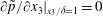 $\partial \tilde{p}/\partial x_{3}|_{x_{3}/{\it\delta}=1}=0$
and
$\partial \tilde{p}/\partial x_{3}|_{x_{3}/{\it\delta}=1}=0$
and
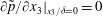 $\partial \tilde{p}/\partial x_{3}|_{x_{3}/{\it\delta}=0}=0$
, respectively. Pseudospectral discretization is used in the horizontal directions, while vertical gradients are evaluated with centred second-order finite differencing.
$\partial \tilde{p}/\partial x_{3}|_{x_{3}/{\it\delta}=0}=0$
, respectively. Pseudospectral discretization is used in the horizontal directions, while vertical gradients are evaluated with centred second-order finite differencing.
The horizontal boundary conditions on the vertical faces of the domain are periodic for all flow quantities, owing to the use of spectral methods in the horizontal directions. At the domain top boundary, the stress-free boundary condition,
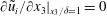 $\partial \tilde{u} _{i}/\partial x_{3}|_{x_{3}/{\it\delta}=1}=0$
for
$\partial \tilde{u} _{i}/\partial x_{3}|_{x_{3}/{\it\delta}=1}=0$
for
 $i=1,2$
, and non-penetration condition for vertical velocity,
$i=1,2$
, and non-penetration condition for vertical velocity,
 $\tilde{u} _{3}|_{x_{3}/{\it\delta}=1}=0$
, are imposed. The Adams–Bashforth time-advancement scheme is used for temporal integration of (A 1). The nonlinear advection term is dealiased in Fourier space with the
$\tilde{u} _{3}|_{x_{3}/{\it\delta}=1}=0$
, are imposed. The Adams–Bashforth time-advancement scheme is used for temporal integration of (A 1). The nonlinear advection term is dealiased in Fourier space with the
 $3/2$
rule (Orszag Reference Orszag1970); this is necessary since aliasing errors may contaminate the smallest resolved scales of the flow, compromising predictions of the SGS models. The numerical scheme is advanced forward in time until the flow field statistics (i.e. Reynolds stresses and kinetic energy) are temporally stationary. We then run the code for an additional averaging period during which turbulence statistics are retrieved. The deviatoric component of
$3/2$
rule (Orszag Reference Orszag1970); this is necessary since aliasing errors may contaminate the smallest resolved scales of the flow, compromising predictions of the SGS models. The numerical scheme is advanced forward in time until the flow field statistics (i.e. Reynolds stresses and kinetic energy) are temporally stationary. We then run the code for an additional averaging period during which turbulence statistics are retrieved. The deviatoric component of
 ${\it\tau}_{ij}$
is evaluated using the eddy viscosity modelling approach,
${\it\tau}_{ij}$
is evaluated using the eddy viscosity modelling approach,
 $$\begin{eqnarray}{\it\tau}_{ij}-{\textstyle \frac{1}{3}}{\it\delta}_{ij}{\it\tau}_{kk}=-2{\it\nu}_{t}\tilde{\unicode[STIX]{x1D61A}}_{ij},\end{eqnarray}$$
where
 ${\it\nu}_{t}=(C_{s}{\it\Delta})^{2}|\tilde{\unicode[STIX]{x1D64E}}|$
is the turbulent viscosity,
${\it\nu}_{t}=(C_{s}{\it\Delta})^{2}|\tilde{\unicode[STIX]{x1D64E}}|$
is the turbulent viscosity,
 $C_{s}$
is the Smagorinsky coefficient (Smagorinsky Reference Smagorinsky1963),
$C_{s}$
is the Smagorinsky coefficient (Smagorinsky Reference Smagorinsky1963),
 ${\it\Delta}$
is the filter size,
${\it\Delta}$
is the filter size,
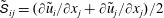 $\tilde{\unicode[STIX]{x1D61A}}_{ij}=(\partial \tilde{u} _{i}/\partial x_{j}+\partial \tilde{u} _{j}/\partial x_{j})/2$
is the resolved strain-rate tensor, and
$\tilde{\unicode[STIX]{x1D61A}}_{ij}=(\partial \tilde{u} _{i}/\partial x_{j}+\partial \tilde{u} _{j}/\partial x_{j})/2$
is the resolved strain-rate tensor, and
 $|\tilde{\unicode[STIX]{x1D64E}}|=(2\tilde{\unicode[STIX]{x1D61A}}_{ij}\tilde{\unicode[STIX]{x1D61A}}_{ij})^{1/2}$
is the magnitude of the resolved strain-rate tensor. In the present study,
$|\tilde{\unicode[STIX]{x1D64E}}|=(2\tilde{\unicode[STIX]{x1D61A}}_{ij}\tilde{\unicode[STIX]{x1D61A}}_{ij})^{1/2}$
is the magnitude of the resolved strain-rate tensor. In the present study,
 $C_{s}$
is evaluated dynamically during LES with the Lagrangian scale-dependent dynamic SGS model of Bou-Zeid et al. (Reference Bou-Zeid, Meneveau and Parlange2005). An additional boundary condition is the imposed surface stress, which occupies two of the deviatoric components of
$C_{s}$
is evaluated dynamically during LES with the Lagrangian scale-dependent dynamic SGS model of Bou-Zeid et al. (Reference Bou-Zeid, Meneveau and Parlange2005). An additional boundary condition is the imposed surface stress, which occupies two of the deviatoric components of
 ${\it\tau}_{ij}$
at
${\it\tau}_{ij}$
at
 $x_{3}/{\it\delta}=0$
,
$x_{3}/{\it\delta}=0$
,
 $$\begin{eqnarray}{\displaystyle \frac{{\it\tau}_{i3}^{w}}{{\it\rho}}}=-\left[{\displaystyle \frac{{\it\kappa}U}{\ln (x_{3}/z_{0}(x_{1},x_{2}))}}\right]^{2}{\displaystyle \frac{\overline{\widehat{\tilde{u} }}_{i}}{U}},\end{eqnarray}$$
where
 $i=1$
and 2,
$i=1$
and 2,
 ${\it\kappa}$
is the von Kármán constant,
${\it\kappa}$
is the von Kármán constant,
 $U=(\overline{\widehat{\tilde{u} }}_{1}^{2}+\overline{\widehat{\tilde{u} }}_{2}^{2})^{1/2}$
is the magnitude of the streamwise and spanwise components of the velocity vector, and the roughness length varies as
$U=(\overline{\widehat{\tilde{u} }}_{1}^{2}+\overline{\widehat{\tilde{u} }}_{2}^{2})^{1/2}$
is the magnitude of the streamwise and spanwise components of the velocity vector, and the roughness length varies as
 $z_{0}(x_{1},x_{2})=z_{0,H}$
or
$z_{0}(x_{1},x_{2})=z_{0,H}$
or
 $z_{0,L}$
, depending on spatial position,
$z_{0,L}$
, depending on spatial position,
 $\{x_{1},x_{2}\}$
, on the figure 1 topography. Here, grid-filtered (
$\{x_{1},x_{2}\}$
, on the figure 1 topography. Here, grid-filtered (
 ${\it\Delta}$
-scale low-pass-filtered), test-filtered (
${\it\Delta}$
-scale low-pass-filtered), test-filtered (
 $2{\it\Delta}$
-scale low-pass-filtered) and test–test-filtered (
$2{\it\Delta}$
-scale low-pass-filtered) and test–test-filtered (
 $4{\it\Delta}$
-scale low-pass-filtered) velocities are denoted by
$4{\it\Delta}$
-scale low-pass-filtered) velocities are denoted by
 $\tilde{u} _{i}$
,
$\tilde{u} _{i}$
,
 $\widehat{\tilde{u} }_{i}$
, and
$\widehat{\tilde{u} }_{i}$
, and
 $\overline{\widehat{\tilde{u} }}_{i}$
, respectively. After Bou-Zeid et al. (Reference Bou-Zeid, Meneveau and Parlange2005), we found that this additional smoothing of input arguments required to compute imposed surface stress helps to preserve numerical stability while using a high-fidelity SGS model. They showed that this approach is advantageous since it removes excessive velocity fluctuations that occur in the vicinity of surface heterogeneities for LES of flows over complex, abruptly varying topographies. In the present study,
$\overline{\widehat{\tilde{u} }}_{i}$
, respectively. After Bou-Zeid et al. (Reference Bou-Zeid, Meneveau and Parlange2005), we found that this additional smoothing of input arguments required to compute imposed surface stress helps to preserve numerical stability while using a high-fidelity SGS model. They showed that this approach is advantageous since it removes excessive velocity fluctuations that occur in the vicinity of surface heterogeneities for LES of flows over complex, abruptly varying topographies. In the present study,
 $x_{i}=\{x_{1},x_{2},x_{3}\}$
and
$x_{i}=\{x_{1},x_{2},x_{3}\}$
and
 $\tilde{u} _{i}=\{\tilde{u} _{1},\tilde{u} _{2},\tilde{u} _{3}\}$
, where subscripts 1, 2 and 3 correspond to the streamwise, spanwise and vertical directions, respectively (see also coordinate system on figure 1
b), and
$\tilde{u} _{i}=\{\tilde{u} _{1},\tilde{u} _{2},\tilde{u} _{3}\}$
, where subscripts 1, 2 and 3 correspond to the streamwise, spanwise and vertical directions, respectively (see also coordinate system on figure 1
b), and
 $\langle {\it\gamma}\rangle _{a}$
denotes averaging of quantity
$\langle {\it\gamma}\rangle _{a}$
denotes averaging of quantity
 ${\it\gamma}$
over dimension
${\it\gamma}$
over dimension
 $a$
. The computational mesh is discretized as
$a$
. The computational mesh is discretized as
 ${\it\Delta}_{x_{1}}=L_{x_{1}}/N_{x_{1}}$
,
${\it\Delta}_{x_{1}}=L_{x_{1}}/N_{x_{1}}$
,
 ${\it\Delta}_{x_{2}}=L_{x_{2}}/N_{x_{2}}$
and
${\it\Delta}_{x_{2}}=L_{x_{2}}/N_{x_{2}}$
and
 ${\it\Delta}_{x_{3}}=L_{x_{3}}/N_{x_{3}}$
, where
${\it\Delta}_{x_{3}}=L_{x_{3}}/N_{x_{3}}$
, where
 $L_{x_{1}}/{\it\delta}=L_{x_{2}}/{\it\delta}=2{\rm\pi}$
,
$L_{x_{1}}/{\it\delta}=L_{x_{2}}/{\it\delta}=2{\rm\pi}$
,
 $N_{x_{1}}=N_{x_{2}}=N_{x_{3}}=64$
and
$N_{x_{1}}=N_{x_{2}}=N_{x_{3}}=64$
and
 $L_{x_{3}}/{\it\delta}=1$
. As the streamwise and spanwise discretizations are equivalent, from this point the nomenclature is simplified by specifying
$L_{x_{3}}/{\it\delta}=1$
. As the streamwise and spanwise discretizations are equivalent, from this point the nomenclature is simplified by specifying
 ${\it\Delta}={\it\Delta}_{x_{1}}={\it\Delta}_{x_{2}}$
. Though the computational mesh is relatively coarse, the present study is theoretical in nature and we found that the resolution was adequate to resolve important details of the flow and allow for long time-averaging periods (Willingham et al.
Reference Willingham, Anderson, Christensen and Barros2013).
${\it\Delta}={\it\Delta}_{x_{1}}={\it\Delta}_{x_{2}}$
. Though the computational mesh is relatively coarse, the present study is theoretical in nature and we found that the resolution was adequate to resolve important details of the flow and allow for long time-averaging periods (Willingham et al.
Reference Willingham, Anderson, Christensen and Barros2013).
Spatial averaging is complicated in the present study owing to the spanwise heterogeneity associated with the LMP–HMP variation (see figure 2 for two-dimensional (2D) illustration of time-averaged 3D velocity field). Thus, the common horizontal statistical homogeneity (HSH) assumption cannot be used here (Belcher, Harman & Finnigan Reference Belcher, Harman and Finnigan2012) to compute turbulence due to resolved motions. Instead, we define the total turbulent (Reynolds) stress
 $\unicode[STIX]{x1D619}_{ij}$
as the combination of SGS and resolved components
$\unicode[STIX]{x1D619}_{ij}$
as the combination of SGS and resolved components
 $$\begin{eqnarray}\unicode[STIX]{x1D619}_{ij}={\it\tau}_{ij}+\tilde{u} _{i}^{\prime }\tilde{u} _{j}^{\prime },\end{eqnarray}$$
where a prime here denotes deviation of a flow quantity,
 ${\it\gamma}$
, from its streamwise (
${\it\gamma}$
, from its streamwise (
 $x_{1}$
) average,
$x_{1}$
) average,
 $$\begin{eqnarray}{\it\gamma}^{\prime }={\it\gamma}-\langle {\it\gamma}\rangle _{1},\end{eqnarray}$$
where averaging of (arbitrary) quantity
 ${\it\gamma}$
with respect to dimension
${\it\gamma}$
with respect to dimension
 $a$
is denoted by
$a$
is denoted by
 $\langle {\it\gamma}\rangle _{a}$
. For instances in which averaging over multiple dimensions is performed,
$\langle {\it\gamma}\rangle _{a}$
. For instances in which averaging over multiple dimensions is performed,
 $\langle {\it\gamma}\rangle _{a,c}$
, the inner- and outermost subscripts correspond to the first and last averaging operations on
$\langle {\it\gamma}\rangle _{a,c}$
, the inner- and outermost subscripts correspond to the first and last averaging operations on
 ${\it\gamma}$
, respectively. Equation (A 5) is thus based on SSH, which is the only permissible spatial averaging operation that can be used to evaluate turbulent stresses associated with resolved scales of the flow.
${\it\gamma}$
, respectively. Equation (A 5) is thus based on SSH, which is the only permissible spatial averaging operation that can be used to evaluate turbulent stresses associated with resolved scales of the flow.
Appendix B. Experimental details
The turbulent boundary layer experiments were conducted in an open-circuit, Eiffel-type, boundary layer wind tunnel. The test section of the tunnel is 6 m long, 45.7 cm tall and 91.4 cm wide, and all boundary layers were formed on a smooth boundary layer plate suspended above the bottom wall of the tunnel. This plate consists of two 3 m long and 91.4 cm wide streamwise-aligned sections smoothly joined at the streamwise centre. Zero-pressure-gradient conditions were achieved via an adjustable ceiling in the test section, and the flow was conditioned upstream of the test section with a series of screens, a honeycomb and a contraction that smoothly guided the flow into the test section. Previous studies provide a more detailed description of this facility and its flow quality (Wu & Christensen Reference Wu and Christensen2006, Reference Wu and Christensen2007, Reference Wu and Christensen2010; Mejia-Alvarez & Christensen Reference Mejia-Alvarez and Christensen2010; Mejia-Alvarez et al. Reference Mejia-Alvarez, Barros and Christensen2013; Mejia-Alvarez & Christensen Reference Mejia-Alvarez and Christensen2013; Barros & Christensen Reference Barros and Christensen2014).
The rough surface used was the same as that originally fabricated and studied by Wu & Christensen (Reference Wu and Christensen2007, Reference Wu and Christensen2010), Mejia-Alvarez & Christensen (Reference Mejia-Alvarez and Christensen2010, Reference Mejia-Alvarez and Christensen2013) and Barros & Christensen (Reference Barros and Christensen2014). This surface is a scaled version of a profilometric surface scan of a turbine blade damaged by the deposition of foreign materials (Bons et al.
Reference Bons, Taylor, McClain and Rivir2001). This topography, shown in perspective view in figure 1(b), is marked by a broad range of topographical scales occurring in a highly irregular arrangement. The average peak-to-valley roughness height of this surface is
 $k=4.25~\text{mm}$
, while the r.m.s. roughness height,
$k=4.25~\text{mm}$
, while the r.m.s. roughness height,
 $k_{rms}$
, is 1.0 mm. As described in Wu & Christensen (Reference Wu and Christensen2007, Reference Wu and Christensen2010), a 3 m long replica of this topography was achieved by mirroring it in both the streamwise and spanwise directions and fabricated with a powder deposition printer. This roughness was mounted on cast aluminium plates and placed along the downstream half of the boundary layer plate, so the boundary layers under study were allowed to initially develop over the first 3 m of the smooth boundary layer plate followed by an additional 3 m of development over the roughness. In all cases, the flow was tripped with a cylindrical rod near the upstream end of the boundary layer plate and all measurements were conducted approximately 2.3 m downstream of the leading edge of the roughness. Wu & Christensen (Reference Wu and Christensen2007) previously reported this rough-wall flow to have achieved self-similar conditions at this measurement location. Table 2 summarizes the experimental parameters of these experiments determined, in part, from the mean velocity profile assessed by ensemble and spanwise averaging the 10 000 PIV velocity fields acquired in this effort (described below).
$k_{rms}$
, is 1.0 mm. As described in Wu & Christensen (Reference Wu and Christensen2007, Reference Wu and Christensen2010), a 3 m long replica of this topography was achieved by mirroring it in both the streamwise and spanwise directions and fabricated with a powder deposition printer. This roughness was mounted on cast aluminium plates and placed along the downstream half of the boundary layer plate, so the boundary layers under study were allowed to initially develop over the first 3 m of the smooth boundary layer plate followed by an additional 3 m of development over the roughness. In all cases, the flow was tripped with a cylindrical rod near the upstream end of the boundary layer plate and all measurements were conducted approximately 2.3 m downstream of the leading edge of the roughness. Wu & Christensen (Reference Wu and Christensen2007) previously reported this rough-wall flow to have achieved self-similar conditions at this measurement location. Table 2 summarizes the experimental parameters of these experiments determined, in part, from the mean velocity profile assessed by ensemble and spanwise averaging the 10 000 PIV velocity fields acquired in this effort (described below).
Table 2. Summary of experimental parameters:
 $U_{e}$
, free-stream velocity;
$U_{e}$
, free-stream velocity;
 $\mathit{Re}_{{\it\theta}}$
, momentum thickness Reynolds number.
$\mathit{Re}_{{\it\theta}}$
, momentum thickness Reynolds number.

Figure 13 presents a schematic of the stereo PIV arrangement for the cross-plane
 $(u_{2}{-}x_{3})$
experiments. Two
$(u_{2}{-}x_{3})$
experiments. Two
 $4000~\text{pixel}\times 2750~\text{pixel}$
, 12 bit, frame-straddle charge-coupled device (CCD) cameras (TSI 11MP) equipped with 180 mm lenses operating at
$4000~\text{pixel}\times 2750~\text{pixel}$
, 12 bit, frame-straddle charge-coupled device (CCD) cameras (TSI 11MP) equipped with 180 mm lenses operating at
 $f\#\,5.6$
imaged the flow field illuminated with a
$f\#\,5.6$
imaged the flow field illuminated with a
 $190~\text{mJ}~\text{pulse}^{-1}$
, dual-cavity pulsed Nd:YAG laser (Quantel). A 1.0 mm thick laser light sheet was formed by three cylindrical lenses and directed into the tunnel’s test section in the
$190~\text{mJ}~\text{pulse}^{-1}$
, dual-cavity pulsed Nd:YAG laser (Quantel). A 1.0 mm thick laser light sheet was formed by three cylindrical lenses and directed into the tunnel’s test section in the
 $x_{2}{-}x_{3}$
plane centred at the midspan of the tunnel. The cameras viewed the
$x_{2}{-}x_{3}$
plane centred at the midspan of the tunnel. The cameras viewed the
 $u_{2}{-}x_{3}$
oriented light sheet from upstream through optical-grade glass side walls of the wind tunnel at angles of
$u_{2}{-}x_{3}$
oriented light sheet from upstream through optical-grade glass side walls of the wind tunnel at angles of
 $\pm 45^{\circ }$
from the streamwise
$\pm 45^{\circ }$
from the streamwise
 $(x_{1})$
direction. In the measurement plane, the angle between each lens and camera CCD array was adjusted to satisfy the Scheimpflug condition ensuring uniform focus across the field of view. The flow was seeded with
$(x_{1})$
direction. In the measurement plane, the angle between each lens and camera CCD array was adjusted to satisfy the Scheimpflug condition ensuring uniform focus across the field of view. The flow was seeded with
 $1~{\rm\mu}\text{m}$
olive-oil droplets generated by a Laskin nozzle, and timing of the cameras, lasers and image acquisition was controlled with a timing unit with 1 ns resolution. Calibration of the stereo imaging system was achieved using a single-plane target with dots spaced at 2.5 mm in both the horizontal and vertical directions. Images of this target were acquired by both cameras at the centre of the laser light sheet and
$1~{\rm\mu}\text{m}$
olive-oil droplets generated by a Laskin nozzle, and timing of the cameras, lasers and image acquisition was controlled with a timing unit with 1 ns resolution. Calibration of the stereo imaging system was achieved using a single-plane target with dots spaced at 2.5 mm in both the horizontal and vertical directions. Images of this target were acquired by both cameras at the centre of the laser light sheet and
 $\pm 250~{\rm\mu}\text{m}$
about the light sheet centre to generate calibration mapping functions from the two 2D image planes to the 3D space defined by the laser light sheet using a least-squares approach.
$\pm 250~{\rm\mu}\text{m}$
about the light sheet centre to generate calibration mapping functions from the two 2D image planes to the 3D space defined by the laser light sheet using a least-squares approach.

Figure 13. Schematic of the experimental arrangement in the cross-flow measurement plane.
Each three-component velocity field was derived from two 2D displacement fields generated from the time-delayed pairs of images acquired by each camera. These pairs of time-delayed images were interrogated in the Insight 3G software package using a recursive two-frame cross-correlation methodology, with a final pass utilizing
 $16^{2}~\text{pixels}$
with 50 % overlap to satisfy the Nyquist sampling criterion. Upon validation of the 2D displacement fields with a median filter and replacement of most erroneous vectors with alternative correlation peaks identified in the interrogation, the final 2D displacement fields contained, on average, only 1–2 % interpolated vectors in regions containing at least 50 % of neighbouring vectors. Each pair of 2D displacement fields was then recombined using the aforementioned mapping function to reconcile all three instantaneous velocity components on the measurement plane defined by the laser light sheet. The field of view was
$16^{2}~\text{pixels}$
with 50 % overlap to satisfy the Nyquist sampling criterion. Upon validation of the 2D displacement fields with a median filter and replacement of most erroneous vectors with alternative correlation peaks identified in the interrogation, the final 2D displacement fields contained, on average, only 1–2 % interpolated vectors in regions containing at least 50 % of neighbouring vectors. Each pair of 2D displacement fields was then recombined using the aforementioned mapping function to reconcile all three instantaneous velocity components on the measurement plane defined by the laser light sheet. The field of view was
 $1.5{\it\delta}\times 3.0{\it\delta}$
(wall normal by spanwise), resulting in a vector grid spacing of
$1.5{\it\delta}\times 3.0{\it\delta}$
(wall normal by spanwise), resulting in a vector grid spacing of
 $520~{\rm\mu}\text{m}~({\sim}30x_{2\ast };x_{2\ast }\approx 17~{\rm\mu}\text{m})$
in both spatial directions. The first grid-point in the wall-normal direction resides at
$520~{\rm\mu}\text{m}~({\sim}30x_{2\ast };x_{2\ast }\approx 17~{\rm\mu}\text{m})$
in both spatial directions. The first grid-point in the wall-normal direction resides at
 $x_{3}/{\it\delta}\simeq 0.07$
relative to the mean elevation of the roughness. A total of 10 000 statistically independent three-component instantaneous velocity fields were acquired at
$x_{3}/{\it\delta}\simeq 0.07$
relative to the mean elevation of the roughness. A total of 10 000 statistically independent three-component instantaneous velocity fields were acquired at
 $\mathit{Re}_{{\it\theta}}\simeq 14\,000$
, and these fields were considered to be statistically independent since the vector field acquisition rate of 0.5 Hz translated to a roughly 35 m (
$\mathit{Re}_{{\it\theta}}\simeq 14\,000$
, and these fields were considered to be statistically independent since the vector field acquisition rate of 0.5 Hz translated to a roughly 35 m (
 ${\sim}350{\it\delta}$
) streamwise ‘separation’ between consecutive fields at the
${\sim}350{\it\delta}$
) streamwise ‘separation’ between consecutive fields at the
 $\mathit{Re}$
studied.
$\mathit{Re}$
studied.
As detailed in Barros (Reference Barros2014), the primary sources of uncertainty in the present experimental dataset arise from the PIV analysis and statistical sampling errors. With respect to the PIV analysis, the random error associated with the subpixel estimator is approximately 5 % of the particle image diameter (2–3 pixels in the present experiments), so approximately 0.15 pixels. In addition, the possibility of peak-locking errors, due to undersampled particle images, must be considered. As outlined in Adrian & Westerweel (Reference Adrian and Westerweel2011), peak-locking uncertainties appear in experiments for which the average particle image diameter is less than 2 pixels. Given an average particle image diameter of 2–3 pixels in this experiment, peak-locking errors are considered negligible. Propagation of the random error of the subpixel estimator and the sampling uncertainty associated with only 10 000 statistically independent fields acquired through the calculated mean and turbulence statistics resulted in relative uncertainties in the mean velocity components of 0.6 % (
 $U_{1}$
) and roughly 3.8 % (
$U_{1}$
) and roughly 3.8 % (
 $U_{2}$
and
$U_{2}$
and
 $U_{3}$
), approximately 3.5 % in each Reynolds normal-stress component and 4.1 %, 8.4 % and 13.6 % in the Reynolds shear-stress components
$U_{3}$
), approximately 3.5 % in each Reynolds normal-stress component and 4.1 %, 8.4 % and 13.6 % in the Reynolds shear-stress components
 $\unicode[STIX]{x1D619}_{13}$
,
$\unicode[STIX]{x1D619}_{13}$
,
 $\unicode[STIX]{x1D619}_{12}$
and
$\unicode[STIX]{x1D619}_{12}$
and
 $\unicode[STIX]{x1D619}_{23}$
, respectively. The reader is directed to Barros (Reference Barros2014) for further details.
$\unicode[STIX]{x1D619}_{23}$
, respectively. The reader is directed to Barros (Reference Barros2014) for further details.


