


1 Introduction
Hydroelastic waves, which describe interactions between deformable ice sheets and water flows beneath, attract a growing interest due to their contribution to climate studies and ice-sheet breakup (Massom et al. Reference Massom, Scambos, Bennetts, Reid, Squire and Stammerjohn2018) and increasing human activities in polar regions. Hydroelastic waves also enjoy a wide range of engineering applications such as airfields built on floating ice, ice breaking with air-cushioned vehicles and manmade very large floating structures. The typical wavelength of hydroelastic waves varies from tens to hundreds of metres, and in consequence, these wave phenomena are easily observable and measurable. A number of field studies have been conducted at McMurdo Sound in Antarctica (Squire et al. Reference Squire, Robinson, Langhorne and Haskell1988) and at Lake Saroma in Hokkaido, Japan (Takizawa Reference Takizawa1985, Reference Takizawa1988). For a quick review, the readers are referred to Ashton (Reference Ashton1986), Squire et al. (Reference Squire, Hosking, Kerr and Langhorne1996), Părău & Dias (Reference Părău and Dias2002) and references therein.
As stated in Korobkin et al. (Reference Korobkin, Părău and Vanden-Broeck2011), a major difficulty with studying hydroelastic waves is the modelling of ice deformations. Linear Euler–Bernoulli beam theory has been intensively used in the early development of hydroelastic waves, where the pressure
 $P$
exerted by the elastic sheet due to flexing is expressed as
$P$
exerted by the elastic sheet due to flexing is expressed as
 $P=D\unicode[STIX]{x1D702}_{xxxx}$
where
$P=D\unicode[STIX]{x1D702}_{xxxx}$
where
 $D$
is the flexural rigidity,
$D$
is the flexural rigidity,
 $x$
is the direction of wave propagation and
$x$
is the direction of wave propagation and
 $\unicode[STIX]{x1D702}$
describes free-surface fluctuations. It is a very good approximation while dealing with small deformations of the elastic cover. The ice breaks due to large wave amplitude where the elastic model is no longer appropriate. By Goodman et al. (Reference Goodman, Wadhams and Squire1980), it happens when the strain in the ice is greater than some critical value that is
$\unicode[STIX]{x1D702}$
describes free-surface fluctuations. It is a very good approximation while dealing with small deformations of the elastic cover. The ice breaks due to large wave amplitude where the elastic model is no longer appropriate. By Goodman et al. (Reference Goodman, Wadhams and Squire1980), it happens when the strain in the ice is greater than some critical value that is
 $4.3\times 10^{-5}$
for sea ice and
$4.3\times 10^{-5}$
for sea ice and
 $2.14\times 10^{-4}$
for pure ice. The monograph by Squire et al. (Reference Squire, Hosking, Kerr and Langhorne1996) summarises linear theories prior to 1996. However the model becomes inaccurate while describing waves of finite amplitude. Observations of intense waves-in-ice events reported by Marko (Reference Marko2003) highlight this limitation. To compute accurately large deformations of the sheet, the nonlinear Kirchhoff–Love (KL) theory of plates was first adopted, where the pressure is in the form of
$2.14\times 10^{-4}$
for pure ice. The monograph by Squire et al. (Reference Squire, Hosking, Kerr and Langhorne1996) summarises linear theories prior to 1996. However the model becomes inaccurate while describing waves of finite amplitude. Observations of intense waves-in-ice events reported by Marko (Reference Marko2003) highlight this limitation. To compute accurately large deformations of the sheet, the nonlinear Kirchhoff–Love (KL) theory of plates was first adopted, where the pressure is in the form of
 $P=D\unicode[STIX]{x1D705}_{xx}$
(
$P=D\unicode[STIX]{x1D705}_{xx}$
(
 $\unicode[STIX]{x1D705}$
is the curvature of the surface). Based on the KL model, Forbes (Reference Forbes1986) computed steady periodic hydroelastic waves of finite amplitude by using a high-order series-expansion technique. For the moving load problem, Părău & Dias (Reference Părău and Dias2002) derived a forced nonlinear Schrödinger equation (NLS), by means of which the authors proved the existence of solitary waves for shallow to moderate water depths. More recently, Milewski et al. (Reference Milewski, Vanden-Broeck and Wang2013) numerically found dark solitary waves and depression generalised solitary waves in deep water in the full Euler equations by using a conformal mapping technique. The existence of these solutions with non-decaying oscillatory tails in the far field was due to the fact that the associated NLS at the bifurcation point is of defocussing type. As a result, free solitary waves can only exist at finite amplitude, and they are numerically found by Milewski et al. (Reference Milewski, Vanden-Broeck and Wang2011). This is in contrast with capillary–gravity solitary waves in deep water bifurcating from infinitesimal periodic waves (Wang & Milewski Reference Wang and Milewski2012). A numerical approach of truncating series was adopted by Vanden-Broeck & Părău (Reference Vanden-Broeck and Părău2011) to compute nonlinear periodic waves and elevation generalised solitary waves in finite-depth water, and infinitely many families of solutions were found.
$\unicode[STIX]{x1D705}$
is the curvature of the surface). Based on the KL model, Forbes (Reference Forbes1986) computed steady periodic hydroelastic waves of finite amplitude by using a high-order series-expansion technique. For the moving load problem, Părău & Dias (Reference Părău and Dias2002) derived a forced nonlinear Schrödinger equation (NLS), by means of which the authors proved the existence of solitary waves for shallow to moderate water depths. More recently, Milewski et al. (Reference Milewski, Vanden-Broeck and Wang2013) numerically found dark solitary waves and depression generalised solitary waves in deep water in the full Euler equations by using a conformal mapping technique. The existence of these solutions with non-decaying oscillatory tails in the far field was due to the fact that the associated NLS at the bifurcation point is of defocussing type. As a result, free solitary waves can only exist at finite amplitude, and they are numerically found by Milewski et al. (Reference Milewski, Vanden-Broeck and Wang2011). This is in contrast with capillary–gravity solitary waves in deep water bifurcating from infinitesimal periodic waves (Wang & Milewski Reference Wang and Milewski2012). A numerical approach of truncating series was adopted by Vanden-Broeck & Părău (Reference Vanden-Broeck and Părău2011) to compute nonlinear periodic waves and elevation generalised solitary waves in finite-depth water, and infinitely many families of solutions were found.
Toland (Reference Toland2007) proposed a novel model on the pressure exerted by the ice sheet based on the Cosserat theory of hyperelastic shells satisfying Kirchhoff’s hypotheses, which takes the form
 $$\begin{eqnarray}\displaystyle P=D\left(\unicode[STIX]{x1D705}_{ss}+{\textstyle \frac{1}{2}}\unicode[STIX]{x1D705}^{3}\right), & & \displaystyle\end{eqnarray}$$
where
 $s$
is the arclength parameter. This new model is consistent with conservation of elastic potential energy and has become the standard model for both theoretical and numerical analyses. Guyenne & Părău (Reference Guyenne and Părău2012) discovered depression and elevation branches of solitary waves below the minimum of the phase speed under this framework. Their results were extended by Wang et al. (Reference Wang, Vanden-Broeck and Milewski2013) to the global bifurcation in the subcritical regime. Gao & Vanden-Broeck (Reference Gao and Vanden-Broeck2014) revisited the problem and showed that elevation generalised solitary waves exist in finite depth but discrete embedded solitons featuring decaying tails were not found. Unsteady computations were performed by Guyenne & Părău (Reference Guyenne and Părău2012) in deep water and by Guyeene & Părău (Reference Guyenne and Părău2014) in shallow water using direct numerical simulations based on the truncated Dirichlet–Neumann operator. The dynamics of hydroelastic solitary waves in the full Euler equations was carried out by Gao et al. (Reference Gao, Wang and Vanden-Broeck2016) in deep water and by Gao et al. (Reference Gao, Vanden-Broeck and Wang2018) for shallow water. In addition, new asymmetric solitary waves were also discovered in this context by the same authors (Gao et al.
Reference Gao, Wang and Vanden-Broeck2016, Reference Gao, Vanden-Broeck and Wang2018). Stability of two-dimensional hydroelastic periodic waves was investigated by Trichtchenko et al. (Reference Trichtchenko, Milewski, Părău and Vanden-Broeck2019) via asymptotic analysis for modulational instability and linear spectral analysis using the Fourier–Floquet–Hill method. Besides, numerical computations were used to analyse high-frequency instabilities in addition to the modulational instability.
$s$
is the arclength parameter. This new model is consistent with conservation of elastic potential energy and has become the standard model for both theoretical and numerical analyses. Guyenne & Părău (Reference Guyenne and Părău2012) discovered depression and elevation branches of solitary waves below the minimum of the phase speed under this framework. Their results were extended by Wang et al. (Reference Wang, Vanden-Broeck and Milewski2013) to the global bifurcation in the subcritical regime. Gao & Vanden-Broeck (Reference Gao and Vanden-Broeck2014) revisited the problem and showed that elevation generalised solitary waves exist in finite depth but discrete embedded solitons featuring decaying tails were not found. Unsteady computations were performed by Guyenne & Părău (Reference Guyenne and Părău2012) in deep water and by Guyeene & Părău (Reference Guyenne and Părău2014) in shallow water using direct numerical simulations based on the truncated Dirichlet–Neumann operator. The dynamics of hydroelastic solitary waves in the full Euler equations was carried out by Gao et al. (Reference Gao, Wang and Vanden-Broeck2016) in deep water and by Gao et al. (Reference Gao, Vanden-Broeck and Wang2018) for shallow water. In addition, new asymmetric solitary waves were also discovered in this context by the same authors (Gao et al.
Reference Gao, Wang and Vanden-Broeck2016, Reference Gao, Vanden-Broeck and Wang2018). Stability of two-dimensional hydroelastic periodic waves was investigated by Trichtchenko et al. (Reference Trichtchenko, Milewski, Părău and Vanden-Broeck2019) via asymptotic analysis for modulational instability and linear spectral analysis using the Fourier–Floquet–Hill method. Besides, numerical computations were used to analyse high-frequency instabilities in addition to the modulational instability.
The aforementioned literature all bear on the irrotational flow of inviscid fluids. However, sea surface waves are frequently accompanied by underlying currents. Currents, the dominant horizontal water movements in the ocean, are normally considered to be steady in view of their large temporal and spatial scales in comparison with surface waves. But in many situations the current velocity in the vertical direction is not constant (e.g. tidal currents and wind-driven currents), and the simplest configuration is a linear shear or constant-vorticity current. Surface gravity waves propagating on linear shear currents were investigated intensively by many authors. Of note are the works of Thomas et al. (Reference Thomas, Kharif and Manna2012) who derived nonlinear Schrödinger equations (such an equation was called a vor-NLS in Thomas et al. (Reference Thomas, Kharif and Manna2012)) to investigate the modulational instability of wavetrains, Francius & Kharif (Reference Francius and Kharif2017) who conducted the stability analysis based on a linear spectral method, Guyenne (Reference Guyenne2017) who proposed a high-order spectral method using the Dirichlet–Neumann operator, Simmen & Saffman (Reference Simmen and Saffman1985), Teles Da Silve & Peregrine (Reference Teles Da Silva and Peregrine1988), Vanden-Broeck (Reference Vanden-Broeck1994) who computed steady periodic waves in the full Euler equations using hodograph transformation and the boundary integral method, Choi (Reference Choi2009) who numerically studied the Benjamin–Feir instability via a time-dependent conformal mapping technique and Riberio et al. (Reference Ribeiro, Milewski and Nachbin2017) who investigated the flow structure beneath rotational water waves. More recently Hsu et al. (Reference Hsu, Kharif, Abid and Chen2018) derived a nonlinear Schrödinger equation for surface capillary–gravity waves on water of finite depth in the presence of constant vorticity to conduct a modulational stability analysis. In the case of three-dimensional space, Milewski & Wang (Reference Milewski and Wang2013) derived a Benney–Roskes–Davey–Stewartson model which was used to compute fully localised lumps. Fully nonlinear computations of the three-dimensional solitary waves were achieved by Trichtchenko et al. (Reference Trichtchenko, Părău, Vanden-Broeck and Milewski2018).
In the context of hydroelastic waves, there is still much to explore in wave–current interactions. Peake (Reference Peake2001, Reference Peake2004) studied the interaction between a uniform current and the elastic plate, and showed that a mean flow has a significant influence on hydroelastic waves. Gao et al. (Reference Gao, Milewski and Vanden-Broeck2019) computed travelling hydroelastic solitary waves and their dynamics in the presence of a linear shear current in the limit of deep water. Bhattacharjee & Sahoo (Reference Bhattacharjee and Sahoo2009) investigated the effect of a linear shear current profile on the propagation of flexural–gravity waves in the linear shallow-water theory, and the transmission and reflection coefficients were derived by imposing conservation of energy flux and the continuity of the vertical deflection of the ice sheet. Another relevant example is the flapping of an elastic plate in a confined channel. It enjoys quite a range of engineering and biomedical applications, for example, energy harvesting devices (Balint & Lucey Reference Balint and Lucey2005; Jaiman et al.
Reference Jaiman, Parmar and Gurugubelli2014; Shoele & Mittal Reference Shoele and Mittal2016). A linear shear current in the presence of viscosity can be achieved experimentally by moving horizontally the rigid bottom with a constant speed (see figure 1
a) or by dragging the plate with a specific value of speed
 $U^{\ast }$
which equals the product of the fixed vorticity and the depth of water (so the velocity at the bottom is zero). A schematic is shown in figure 1.
$U^{\ast }$
which equals the product of the fixed vorticity and the depth of water (so the velocity at the bottom is zero). A schematic is shown in figure 1.

Figure 1. Schematic of the relevant problems.
In this work, we are concerned with hydroelastic waves on water of finite depth interacting with a linear shear current in inviscid flows. We derive a nonlinear Schrödinger equation for quasi-monochromatic wavetrains and discuss the various behaviours of the coefficient of the nonlinear term from the NLS at different parameter values. Fully nonlinear computations of solitary waves, as well as the Benjamin–Feir instability, are performed to validate the predictions of the NLS and describe behaviour beyond its applicability. The rest of the paper is structured as follows. The mathematical formulation of the problem is presented in § 2, following by the derivation of the NLS in § 3, analysis of the modulational instability in § 4 and the numerical scheme for the primitive equations in § 5. The fully nonlinear results are presented in § 6, and a conclusion is given in § 7.
2 Mathematical formulation
We consider an incompressible flow of an inviscid fluid in a two-dimensional Cartesian coordinate system, where gravity points in the negative
 $y$
direction. The velocity field is denoted
$y$
direction. The velocity field is denoted
 $(u,v)$
in the fluid region bounded below by the horizontal rigid bottom
$(u,v)$
in the fluid region bounded below by the horizontal rigid bottom
 $y=-h$
and above by the elastic sheet
$y=-h$
and above by the elastic sheet
 $y=\unicode[STIX]{x1D702}(x,t)$
. The Euler equations governing the motion of an ideal fluid body are
$y=\unicode[STIX]{x1D702}(x,t)$
. The Euler equations governing the motion of an ideal fluid body are
 $$\begin{eqnarray}\displaystyle & \displaystyle \frac{\unicode[STIX]{x2202}u}{\unicode[STIX]{x2202}x}+\frac{\unicode[STIX]{x2202}v}{\unicode[STIX]{x2202}y}=0, & \displaystyle\end{eqnarray}$$
 $$\begin{eqnarray}\displaystyle & \displaystyle \frac{\unicode[STIX]{x2202}u}{\unicode[STIX]{x2202}t}+u\frac{\unicode[STIX]{x2202}u}{\unicode[STIX]{x2202}x}+v\frac{\unicode[STIX]{x2202}u}{\unicode[STIX]{x2202}y}=-\frac{P_{x}}{\unicode[STIX]{x1D70C}}, & \displaystyle\end{eqnarray}$$
 $$\begin{eqnarray}\displaystyle & \displaystyle \frac{\unicode[STIX]{x2202}v}{\unicode[STIX]{x2202}t}+u\frac{\unicode[STIX]{x2202}v}{\unicode[STIX]{x2202}x}+v\frac{\unicode[STIX]{x2202}v}{\unicode[STIX]{x2202}y}=-\frac{P_{y}}{\unicode[STIX]{x1D70C}}-g, & \displaystyle\end{eqnarray}$$
where
 $P$
is the pressure,
$P$
is the pressure,
 $\unicode[STIX]{x1D70C}$
the density of the fluid and
$\unicode[STIX]{x1D70C}$
the density of the fluid and
 $g$
the acceleration due to gravity. The boundary conditions of the present problem are
$g$
the acceleration due to gravity. The boundary conditions of the present problem are
 $$\begin{eqnarray}\displaystyle \left.\begin{array}{@{}c@{}}\displaystyle v=\unicode[STIX]{x1D702}_{t}+u\unicode[STIX]{x1D702}_{x},\quad \text{at }y=\unicode[STIX]{x1D702}(x,t),\\ \displaystyle P-P_{atm}=D\left(\unicode[STIX]{x1D705}_{ss}+\frac{\unicode[STIX]{x1D705}^{3}}{2}\right),\quad \text{at }y=\unicode[STIX]{x1D702}(x,t),\\ \displaystyle v=0,\quad \text{at }y=-h,\end{array}\right\} & & \displaystyle\end{eqnarray}$$
where
 $D$
is the flexural rigidity of the elastic cover and
$D$
is the flexural rigidity of the elastic cover and
 $P_{atm}$
is the atmospheric pressure, assumed to be zero. Here
$P_{atm}$
is the atmospheric pressure, assumed to be zero. Here
 $\unicode[STIX]{x1D705}$
is the curvature of the deformable sheet, and
$\unicode[STIX]{x1D705}$
is the curvature of the deformable sheet, and
 $\unicode[STIX]{x1D705}_{ss}$
is its second derivative with respect to the arclength parameter
$\unicode[STIX]{x1D705}_{ss}$
is its second derivative with respect to the arclength parameter
 $s$
. The vorticity is denoted by
$s$
. The vorticity is denoted by
 $$\begin{eqnarray}\displaystyle \unicode[STIX]{x1D6FA}\,\triangleq \,\frac{\unicode[STIX]{x2202}v}{\unicode[STIX]{x2202}x}-\frac{\unicode[STIX]{x2202}u}{\unicode[STIX]{x2202}y}. & & \displaystyle\end{eqnarray}$$
The governing equation for the vorticity
 $$\begin{eqnarray}\displaystyle \unicode[STIX]{x1D6FA}_{t}+u\unicode[STIX]{x1D6FA}_{x}+v\unicode[STIX]{x1D6FA}_{y}=0, & & \displaystyle\end{eqnarray}$$
indicates that if the initial vorticity is constant everywhere in the fluid body, it remains unchanged as time evolves. By assuming a constant vorticity
 $\unicode[STIX]{x1D6FA}=\unicode[STIX]{x1D6FA}_{0}$
, it can be easily checked that
$\unicode[STIX]{x1D6FA}=\unicode[STIX]{x1D6FA}_{0}$
, it can be easily checked that
 $$\begin{eqnarray}\displaystyle (u_{0},v_{0})=(U_{0}-\unicode[STIX]{x1D6FA}_{0}y,0),\quad \text{in }-h<y<0, & & \displaystyle\end{eqnarray}$$
is a solution to the Euler equations, satisfying all boundary conditions, where
 $U_{0}$
is a constant velocity at
$U_{0}$
is a constant velocity at
 $y=0$
. For this two-dimensional problem, we assume that the velocity field is an irrotational perturbation of the linear shear current, namely,
$y=0$
. For this two-dimensional problem, we assume that the velocity field is an irrotational perturbation of the linear shear current, namely,
 $$\begin{eqnarray}\displaystyle (u,v)=(u_{0},v_{0})+\unicode[STIX]{x1D735}\unicode[STIX]{x1D719}, & & \displaystyle\end{eqnarray}$$
where
 $\unicode[STIX]{x1D719}$
is the potential function of the irrotational part (a schematic description is shown in figure 2). Substituting (2.8) into (2.1)–(2.4) yields
$\unicode[STIX]{x1D719}$
is the potential function of the irrotational part (a schematic description is shown in figure 2). Substituting (2.8) into (2.1)–(2.4) yields
 $$\begin{eqnarray}\left.\begin{array}{@{}c@{}}\displaystyle \unicode[STIX]{x1D719}_{xx}+\unicode[STIX]{x1D719}_{yy}=0,\quad \text{for }-h<y<\unicode[STIX]{x1D702}(x,t),\\ \displaystyle \unicode[STIX]{x1D719}_{y}=0,\quad \text{at }y=-h,\\ \displaystyle \unicode[STIX]{x1D702}_{t}=\unicode[STIX]{x1D719}_{y}-\unicode[STIX]{x1D702}_{x}\left(u_{0}+\unicode[STIX]{x1D719}_{x}\right),\quad \text{at }y=\unicode[STIX]{x1D702}(x,t),\\ \displaystyle \unicode[STIX]{x1D719}_{t}+u_{0}\unicode[STIX]{x1D719}_{x}+\frac{1}{2}\left|\unicode[STIX]{x1D735}\unicode[STIX]{x1D719}\right|^{2}+\unicode[STIX]{x1D6FA}_{0}\unicode[STIX]{x1D713}+g\unicode[STIX]{x1D702}+\frac{D}{\unicode[STIX]{x1D70C}}\left[\frac{1}{2}\unicode[STIX]{x1D705}^{3}+\unicode[STIX]{x1D705}_{ss}\right]=B(t),\quad \text{at }y=\unicode[STIX]{x1D702}(x,t),\end{array}\right\}\end{eqnarray}$$
where
 $\unicode[STIX]{x1D713}$
is the streamfunction of the fluid, and the harmonic conjugate of
$\unicode[STIX]{x1D713}$
is the streamfunction of the fluid, and the harmonic conjugate of
 $\unicode[STIX]{x1D719}$
as well. It is noted that the integral constant
$\unicode[STIX]{x1D719}$
as well. It is noted that the integral constant
 $B(t)$
can be absorbed by redefining the velocity potential
$B(t)$
can be absorbed by redefining the velocity potential
 $\unicode[STIX]{x1D719}$
, and we can always assume
$\unicode[STIX]{x1D719}$
, and we can always assume
 $U_{0}=0$
through a moving frame of reference.
$U_{0}=0$
through a moving frame of reference.

Figure 2. Schematic description of the present problem.
3 Normal form analysis
In this section, we sketch the derivation of the cubic nonlinear Schrödinger equation and related modulational approximations by the method of multiple scales. By taking the derivative of the last equation of (2.9) with respect to
 $x$
and making use of the Cauchy–Riemann relation to eliminate
$x$
and making use of the Cauchy–Riemann relation to eliminate
 $\unicode[STIX]{x1D713}$
, we arrive at
$\unicode[STIX]{x1D713}$
, we arrive at
 $$\begin{eqnarray}\displaystyle & & \displaystyle \unicode[STIX]{x1D719}_{tx}+\unicode[STIX]{x1D702}_{x}\unicode[STIX]{x1D719}_{ty}+\unicode[STIX]{x1D719}_{x}(\unicode[STIX]{x1D719}_{xx}+\unicode[STIX]{x1D702}_{x}\unicode[STIX]{x1D719}_{xy})+\unicode[STIX]{x1D719}_{y}(\unicode[STIX]{x1D719}_{xy}+\unicode[STIX]{x1D702}_{x}\unicode[STIX]{x1D719}_{yy})-\unicode[STIX]{x1D6FA}_{0}\unicode[STIX]{x1D702}(\unicode[STIX]{x1D719}_{xx}+\unicode[STIX]{x1D702}_{x}\unicode[STIX]{x1D719}_{xy})\nonumber\\ \displaystyle & & \displaystyle \qquad -\,\unicode[STIX]{x1D6FA}_{0}\unicode[STIX]{x1D702}_{x}\unicode[STIX]{x1D719}_{x}+\unicode[STIX]{x1D6FA}_{0}(-\unicode[STIX]{x1D719}_{y}+\unicode[STIX]{x1D702}_{x}\unicode[STIX]{x1D719}_{x})+g\unicode[STIX]{x1D702}_{x}+\frac{D}{\unicode[STIX]{x1D70C}}\left[\frac{1}{2}\unicode[STIX]{x1D705}^{3}+\unicode[STIX]{x1D705}_{ss}\right]_{x}=0.\end{eqnarray}$$
For a weakly nonlinear wavetrain, we can assume
 $\unicode[STIX]{x1D719}$
and
$\unicode[STIX]{x1D719}$
and
 $\unicode[STIX]{x1D702}$
are of order
$\unicode[STIX]{x1D702}$
are of order
 $\unicode[STIX]{x1D716}$
, where
$\unicode[STIX]{x1D716}$
, where
 $\unicode[STIX]{x1D716}$
is a positive small parameter that measures the wave slope. It follows that the velocity potential on the free surface can be expanded about
$\unicode[STIX]{x1D716}$
is a positive small parameter that measures the wave slope. It follows that the velocity potential on the free surface can be expanded about
 $y=0$
as
$y=0$
as
 $$\begin{eqnarray}\displaystyle \unicode[STIX]{x1D719}(x,\unicode[STIX]{x1D702},t)=\unicode[STIX]{x1D719}(x,0,t)+\unicode[STIX]{x1D702}\unicode[STIX]{x1D719}_{y}(x,0,t)+\frac{\unicode[STIX]{x1D702}^{2}}{2}\unicode[STIX]{x1D719}_{yy}(x,0,t)+O(\unicode[STIX]{x1D716}^{4}). & & \displaystyle\end{eqnarray}$$
Therefore expanding the kinematic and dynamic boundary conditions about
 $y=0$
yields
$y=0$
yields
 $$\begin{eqnarray}\displaystyle \unicode[STIX]{x1D702}_{t}-\unicode[STIX]{x1D719}_{y}=\unicode[STIX]{x1D702}\unicode[STIX]{x1D719}_{yy}-\unicode[STIX]{x1D702}_{x}\unicode[STIX]{x1D719}_{x}+\unicode[STIX]{x1D6FA}_{0}\unicode[STIX]{x1D702}\unicode[STIX]{x1D702}_{x}+\frac{\unicode[STIX]{x1D702}^{2}}{2}\unicode[STIX]{x1D719}_{yyy}-\unicode[STIX]{x1D702}\unicode[STIX]{x1D702}_{x}\unicode[STIX]{x1D719}_{xy}, & & \displaystyle\end{eqnarray}$$
 $$\begin{eqnarray}\displaystyle & & \displaystyle g\unicode[STIX]{x1D702}_{x}+\frac{D}{\unicode[STIX]{x1D70C}}\unicode[STIX]{x1D702}_{xxxxx}+\unicode[STIX]{x1D719}_{tx}-\unicode[STIX]{x1D6FA}_{0}\unicode[STIX]{x1D719}_{y}\nonumber\\ \displaystyle & & \displaystyle \qquad =-\unicode[STIX]{x1D702}\unicode[STIX]{x1D719}_{txy}-\unicode[STIX]{x1D702}_{x}\unicode[STIX]{x1D719}_{ty}-\unicode[STIX]{x1D719}_{x}\unicode[STIX]{x1D719}_{xx}-\unicode[STIX]{x1D719}_{y}\unicode[STIX]{x1D719}_{xy}+\unicode[STIX]{x1D6FA}_{0}\unicode[STIX]{x1D702}\unicode[STIX]{x1D719}_{xx}+\unicode[STIX]{x1D6FA}_{0}\unicode[STIX]{x1D702}\unicode[STIX]{x1D719}_{yy}-\frac{\unicode[STIX]{x1D702}^{2}}{2}\unicode[STIX]{x1D719}_{txyy}-\unicode[STIX]{x1D702}\unicode[STIX]{x1D702}_{x}\unicode[STIX]{x1D719}_{tyy}\nonumber\\ \displaystyle & & \displaystyle \qquad \quad -\,\unicode[STIX]{x1D702}\unicode[STIX]{x1D719}_{x}\unicode[STIX]{x1D719}_{xxy}-\unicode[STIX]{x1D702}_{x}\unicode[STIX]{x1D719}_{x}\unicode[STIX]{x1D719}_{xy}-\unicode[STIX]{x1D702}\unicode[STIX]{x1D719}_{y}\unicode[STIX]{x1D719}_{xyy}-\unicode[STIX]{x1D702}_{x}\unicode[STIX]{x1D719}_{y}\unicode[STIX]{x1D719}_{yy}+\unicode[STIX]{x1D6FA}_{0}\left[\unicode[STIX]{x1D702}^{2}\unicode[STIX]{x1D719}_{xxy}+\unicode[STIX]{x1D702}\unicode[STIX]{x1D702}_{x}\unicode[STIX]{x1D719}_{xy}+\frac{\unicode[STIX]{x1D702}^{2}}{2}\unicode[STIX]{x1D719}_{yyy}\right]\nonumber\\ \displaystyle & & \displaystyle \qquad \quad +\,\frac{D}{\unicode[STIX]{x1D70C}}\unicode[STIX]{x2202}_{x}\left[\frac{5}{2}\unicode[STIX]{x1D702}_{x}^{2}\unicode[STIX]{x1D702}_{xxxx}+\frac{5}{2}\unicode[STIX]{x1D702}_{xx}^{3}+10\unicode[STIX]{x1D702}_{x}\unicode[STIX]{x1D702}_{xx}\unicode[STIX]{x1D702}_{xxx}\right].\end{eqnarray}$$
Here we retain the terms valid up to the third order of
 $\unicode[STIX]{x1D716}$
which is sufficient for our purposes. We now consider the development of a fast oscillatory wavetrain whose envelope features a slowly evolving structure. To derive the governing equation of the wave envelope, we introduce ‘slow’ variables
$\unicode[STIX]{x1D716}$
which is sufficient for our purposes. We now consider the development of a fast oscillatory wavetrain whose envelope features a slowly evolving structure. To derive the governing equation of the wave envelope, we introduce ‘slow’ variables
 $X=\unicode[STIX]{x1D716}x$
,
$X=\unicode[STIX]{x1D716}x$
,
 $T=\unicode[STIX]{x1D716}t$
and
$T=\unicode[STIX]{x1D716}t$
and
 $\unicode[STIX]{x1D70F}=\unicode[STIX]{x1D716}^{2}t$
, and pick
$\unicode[STIX]{x1D70F}=\unicode[STIX]{x1D716}^{2}t$
, and pick
 $\text{e}^{\text{i}(kx-\unicode[STIX]{x1D714}t)}$
as the carrying wave. Three distinct cases will arise out of the analysis: the general case (denoted ‘non-resonant’ below) and two resonant cases: the Wilton-ripple-like resonance where the harmonic is resonant with the carrier wave and the long-wave/short-wave resonance where the mean flow induced by the carrier wave is resonant with the long-wave mode of the system.
$\text{e}^{\text{i}(kx-\unicode[STIX]{x1D714}t)}$
as the carrying wave. Three distinct cases will arise out of the analysis: the general case (denoted ‘non-resonant’ below) and two resonant cases: the Wilton-ripple-like resonance where the harmonic is resonant with the carrier wave and the long-wave/short-wave resonance where the mean flow induced by the carrier wave is resonant with the long-wave mode of the system.
3.1 Non-resonant case
The derivation of the standard NLS is well documented (Davey & Stewartson Reference Davey and Stewartson1974; Djordjevic & Redekopp Reference Djordjevic and Redekopp1977) and therefore omitted here. Some intermediate results can be found in appendix A. Substituting the ansatz
 $$\begin{eqnarray}\displaystyle & \displaystyle \unicode[STIX]{x1D702}=\unicode[STIX]{x1D716}A_{11}(X-c_{g}T,\unicode[STIX]{x1D70F})\text{e}^{\text{i}\unicode[STIX]{x1D6E9}}+\mathop{\sum }_{n=2}^{\infty }\unicode[STIX]{x1D716}^{n}\mathop{\sum }_{j=0}^{n}A_{nj}\left(X-c_{g}T,\unicode[STIX]{x1D70F}\right)\text{e}^{j\text{i}\unicode[STIX]{x1D6E9}}+\text{c.c.}, & \displaystyle\end{eqnarray}$$
 $$\begin{eqnarray}\displaystyle & \displaystyle \unicode[STIX]{x1D719}=\mathop{\sum }_{n=1}^{\infty }\unicode[STIX]{x1D716}^{n}\mathop{\sum }_{j=0}^{n}\unicode[STIX]{x1D719}_{nj}(X-c_{g}T,y,\unicode[STIX]{x1D70F})\text{e}^{j\text{i}\unicode[STIX]{x1D6E9}}+\text{c.c.}, & \displaystyle\end{eqnarray}$$
where
 $\unicode[STIX]{x1D6E9}=kx-\unicode[STIX]{x1D714}t$
and c.c. represents the complex conjugate into the kinematic and dynamic boundary conditions (3.3)–(3.4) yields at the leading order,
$\unicode[STIX]{x1D6E9}=kx-\unicode[STIX]{x1D714}t$
and c.c. represents the complex conjugate into the kinematic and dynamic boundary conditions (3.3)–(3.4) yields at the leading order,
 $$\begin{eqnarray}\displaystyle \left.\begin{array}{@{}c@{}}\displaystyle \text{i}\unicode[STIX]{x1D714}A_{11}+k\sinh (kh)\unicode[STIX]{x1D711}_{11}=0,\\ \displaystyle \text{i}\left(gk+\frac{D}{\unicode[STIX]{x1D70C}}k^{5}\right)A_{11}+[\unicode[STIX]{x1D714}k\cosh (kh)-\unicode[STIX]{x1D6FA}_{0}k\sinh (kh)]\unicode[STIX]{x1D711}_{11}=0,\end{array}\right\} & & \displaystyle\end{eqnarray}$$
where
 $\unicode[STIX]{x1D711}_{11}=\unicode[STIX]{x1D719}_{11}/\cosh (k(y+h))$
. The existence of a non-zero solution results in the dispersion relation
$\unicode[STIX]{x1D711}_{11}=\unicode[STIX]{x1D719}_{11}/\cosh (k(y+h))$
. The existence of a non-zero solution results in the dispersion relation
 $$\begin{eqnarray}\displaystyle \unicode[STIX]{x1D714}^{2}-\unicode[STIX]{x1D6FA}_{0}\tanh (kh)\unicode[STIX]{x1D714}-k\tanh (kh)\left(g+\frac{D}{\unicode[STIX]{x1D70C}}k^{4}\right)=0. & & \displaystyle\end{eqnarray}$$
At the second order, one gets
 $$\begin{eqnarray}\displaystyle (A_{11})_{T}+c_{g}(A_{11})_{X}=0, & & \displaystyle\end{eqnarray}$$
where
 $c_{g}=\unicode[STIX]{x1D714}_{k}$
is the group speed (its explicit form is presented in (A 7) in appendix A). At the cubic order, after a considerable amount of algebra, one obtains the solvability conditions that result in the equations governing the relation between the mean flow
$c_{g}=\unicode[STIX]{x1D714}_{k}$
is the group speed (its explicit form is presented in (A 7) in appendix A). At the cubic order, after a considerable amount of algebra, one obtains the solvability conditions that result in the equations governing the relation between the mean flow
 $\unicode[STIX]{x1D719}_{10}$
and the carrier wave amplitude
$\unicode[STIX]{x1D719}_{10}$
and the carrier wave amplitude
 $A_{11}$
 $$\begin{eqnarray}\displaystyle [c_{g}(c_{g}-\unicode[STIX]{x1D6FA}_{0}h)-gh]{\unicode[STIX]{x1D719}_{10}}_{X}=\left[\frac{2g\unicode[STIX]{x1D714}}{\tanh (kh)}+\frac{c_{g}\unicode[STIX]{x1D714}^{2}}{\sinh ^{2}(kh)}\right]|A_{11}|^{2}, & & \displaystyle\end{eqnarray}$$
and the equation for the modulation of the carrier wave
 $$\begin{eqnarray}\displaystyle \text{i}A_{11_{\unicode[STIX]{x1D70F}}}+\unicode[STIX]{x1D706}A_{11_{XX}}+\frac{\unicode[STIX]{x1D6FC}_{1}}{2\unicode[STIX]{x1D714}^{2}\coth (kh)-\unicode[STIX]{x1D6FA}_{0}\unicode[STIX]{x1D714}}A_{11}{\unicode[STIX]{x1D719}_{10}}_{X}+\frac{\unicode[STIX]{x1D6FC}_{2}}{2\unicode[STIX]{x1D714}^{2}\coth (kh)-\unicode[STIX]{x1D6FA}_{0}\unicode[STIX]{x1D714}}|A_{11}|^{2}A_{11}=0, & & \displaystyle \nonumber\\ \displaystyle & & \displaystyle\end{eqnarray}$$
where
 $$\begin{eqnarray}\displaystyle & \displaystyle \unicode[STIX]{x1D706}=\frac{\unicode[STIX]{x1D714}_{kk}}{2}, & \displaystyle\end{eqnarray}$$
 $$\begin{eqnarray}\displaystyle & \displaystyle \unicode[STIX]{x1D6FC}_{1}=-k\unicode[STIX]{x1D714}\left\{\frac{h\unicode[STIX]{x1D714}^{2}}{c_{g}\sinh ^{2}(kh)}+\left(1-\frac{h\unicode[STIX]{x1D6FA}_{0}}{c_{g}}\right)[2\unicode[STIX]{x1D714}\coth (kh)-\unicode[STIX]{x1D6FA}_{0}]\right\} & \displaystyle\end{eqnarray}$$
 $$\begin{eqnarray}\displaystyle \unicode[STIX]{x1D6FC}_{2} & = & \displaystyle -\frac{2k\unicode[STIX]{x1D714}^{2}}{c_{g}\tanh (kh)}\left[\frac{\unicode[STIX]{x1D714}^{2}}{\sinh ^{2}(kh)}-2\unicode[STIX]{x1D6FA}_{0}\unicode[STIX]{x1D714}\coth (kh)+\unicode[STIX]{x1D6FA}_{0}^{2}\right]\nonumber\\ \displaystyle & & \displaystyle -\,k\unicode[STIX]{x1D714}\left[\frac{\unicode[STIX]{x1D714}^{2}}{\sinh ^{2}(kh)}-2\unicode[STIX]{x1D6FA}_{0}\unicode[STIX]{x1D714}\coth (kh)+\unicode[STIX]{x1D6FA}_{0}^{2}\right]\frac{D_{1}}{D_{0}}\nonumber\\ \displaystyle & & \displaystyle +\,2k^{2}\unicode[STIX]{x1D714}[2\unicode[STIX]{x1D714}\coth (kh)-\unicode[STIX]{x1D6FA}_{0}]\cosh (2kh)\frac{D_{2}}{\text{i}D_{0}}-2k^{2}\unicode[STIX]{x1D714}^{2}\sinh (2kh)\frac{D_{2}}{\text{i}D_{0}}\nonumber\\ \displaystyle & & \displaystyle -\,4k^{2}\unicode[STIX]{x1D714}^{3}\coth (kh)+3\unicode[STIX]{x1D6FA}_{0}k^{2}\unicode[STIX]{x1D714}^{2}+\frac{5D}{\unicode[STIX]{x1D70C}}k^{7}\unicode[STIX]{x1D714}.\end{eqnarray}$$
The explicit form of
 $D_{0}$
,
$D_{0}$
,
 $D_{1}$
and
$D_{1}$
and
 $D_{2}$
can be found in appendix A. Combining (3.10) and (3.11) yields a single equation for the envelope
$D_{2}$
can be found in appendix A. Combining (3.10) and (3.11) yields a single equation for the envelope
 $A_{11}$
(for the sake of simple notations, we write
$A_{11}$
(for the sake of simple notations, we write
 $A$
at the place of
$A$
at the place of
 $A_{11}$
),
$A_{11}$
),
 $$\begin{eqnarray}\displaystyle \text{i}A_{\unicode[STIX]{x1D70F}}+\unicode[STIX]{x1D706}A_{XX}+\frac{\unicode[STIX]{x1D6FC}}{2\unicode[STIX]{x1D714}^{2}\coth (kh)-\unicode[STIX]{x1D6FA}_{0}\unicode[STIX]{x1D714}}|A|^{2}A=0, & & \displaystyle\end{eqnarray}$$
where
 $$\begin{eqnarray}\displaystyle \unicode[STIX]{x1D6FC}=\unicode[STIX]{x1D6FC}_{2}+\unicode[STIX]{x1D6FC}_{1}\left.\left[{\displaystyle \frac{2g\unicode[STIX]{x1D714}}{\tanh (kh)}}+{\displaystyle \frac{c_{g}\unicode[STIX]{x1D714}^{2}}{\sinh ^{2}(kh)}}\right]\right/[c_{g}(c_{g}-\unicode[STIX]{x1D6FA}_{0}h)-gh]. & & \displaystyle\end{eqnarray}$$
Equation (3.15) matches with Thomas et al. (Reference Thomas, Kharif and Manna2012) in the case of gravity waves with vorticity where
 $D=0$
. We call (3.15) the vor-NLS which reduces to the form in Milewski & Wang (Reference Milewski and Wang2013) in absence of the linear shear current and for a one-dimensional free surface.
$D=0$
. We call (3.15) the vor-NLS which reduces to the form in Milewski & Wang (Reference Milewski and Wang2013) in absence of the linear shear current and for a one-dimensional free surface.
3.2 Second harmonic resonance
The second harmonic resonance takes place when a wave of a specific wavenumber
 $k^{\dagger }$
propagates at the identical speed of its second harmonic, i.e.
$k^{\dagger }$
propagates at the identical speed of its second harmonic, i.e.
 $\unicode[STIX]{x1D714}(2k^{\dagger })=2\unicode[STIX]{x1D714}(k^{\dagger })$
, or equivalently
$\unicode[STIX]{x1D714}(2k^{\dagger })=2\unicode[STIX]{x1D714}(k^{\dagger })$
, or equivalently
 $$\begin{eqnarray}\displaystyle \tanh (k^{\dagger }h)\unicode[STIX]{x1D714}^{2}(k^{\dagger })-\frac{15D}{\unicode[STIX]{x1D70C}}(k^{\dagger })^{5}=0. & & \displaystyle\end{eqnarray}$$
This condition for capillary–gravity waves gives rise to the Wilton ripples (Wilton Reference Wilton1915). The coefficient
 $\unicode[STIX]{x1D6FC}$
of the nonlinear term from the vor-NLS (3.15) becomes singular due to
$\unicode[STIX]{x1D6FC}$
of the nonlinear term from the vor-NLS (3.15) becomes singular due to
 $D_{0}=0$
. A modified multi-scale analysis is required, including the harmonic mode
$D_{0}=0$
. A modified multi-scale analysis is required, including the harmonic mode
 $2$
in the leading order, and obtaining solvability conditions at quadratic order. The expansion of
$2$
in the leading order, and obtaining solvability conditions at quadratic order. The expansion of
 $\unicode[STIX]{x1D702}$
up to
$\unicode[STIX]{x1D702}$
up to
 $\unicode[STIX]{x1D716}^{2}$
is therefore
$\unicode[STIX]{x1D716}^{2}$
is therefore
 $$\begin{eqnarray}\displaystyle \unicode[STIX]{x1D702} & = & \displaystyle \unicode[STIX]{x1D716}A_{11}(X,T)\text{e}^{\text{i}\unicode[STIX]{x1D6E9}}+\unicode[STIX]{x1D716}A_{12}(X,T)\text{e}^{2\text{i}\unicode[STIX]{x1D6E9}}+\unicode[STIX]{x1D716}^{2}A_{21}(X,T)\text{e}^{\text{i}\unicode[STIX]{x1D6E9}}\nonumber\\ \displaystyle & & \displaystyle +\,\unicode[STIX]{x1D716}^{2}A_{22}(X,T)\text{e}^{2\text{i}\unicode[STIX]{x1D6E9}}+\cdots +\text{c.c.},\end{eqnarray}$$
with a corresponding expansion for
 $\unicode[STIX]{x1D719}$
. Solving the Laplace equation with the kinematic boundary condition on the bottom yields
$\unicode[STIX]{x1D719}$
. Solving the Laplace equation with the kinematic boundary condition on the bottom yields
 $$\begin{eqnarray}\displaystyle \unicode[STIX]{x1D719} & = & \displaystyle \unicode[STIX]{x1D716}\unicode[STIX]{x1D711}_{10}+\unicode[STIX]{x1D716}\unicode[STIX]{x1D711}_{11}(X,T)\cosh (k(y+h))\text{e}^{\text{i}\unicode[STIX]{x1D6E9}}+\unicode[STIX]{x1D716}\unicode[STIX]{x1D711}_{12}(X,T)\cosh (2k(y+h))\text{e}^{2\text{i}\unicode[STIX]{x1D6E9}}\nonumber\\ \displaystyle & & \displaystyle +\,\unicode[STIX]{x1D716}^{2}\unicode[STIX]{x1D711}_{20}+\unicode[STIX]{x1D716}^{2}[\unicode[STIX]{x1D711}_{21}(X,T)\cosh (k(y+h))-\text{i}(y+h)\sinh (k(y+h))]\text{e}^{\text{i}\unicode[STIX]{x1D6E9}}\nonumber\\ \displaystyle & & \displaystyle +\,\unicode[STIX]{x1D716}^{2}[\unicode[STIX]{x1D711}_{22}(X,T)\cosh (2k(y+h))-\text{i}(y+h)\sinh (2k(y+h))]\text{e}^{2\text{i}\unicode[STIX]{x1D6E9}}+\cdots +\text{c.c.}\nonumber\\ \displaystyle & & \displaystyle\end{eqnarray}$$
We perform similar calculations as presented in McGoldrick (Reference McGoldrick1970) or Jones (Reference Jones1992) by substituting the ansatz (3.18)–(3.19) into boundary conditions (3.3), (3.4) and collecting the coefficients of
 $\unicode[STIX]{x1D716}^{2}\text{e}^{\text{i}\unicode[STIX]{x1D6E9}}$
and
$\unicode[STIX]{x1D716}^{2}\text{e}^{\text{i}\unicode[STIX]{x1D6E9}}$
and
 $\unicode[STIX]{x1D716}^{2}\text{e}^{2\text{i}\unicode[STIX]{x1D6E9}}$
. At the leading order, the solvability conditions for the first harmonic and the second harmonic give two separate equations
$\unicode[STIX]{x1D716}^{2}\text{e}^{2\text{i}\unicode[STIX]{x1D6E9}}$
. At the leading order, the solvability conditions for the first harmonic and the second harmonic give two separate equations
 $$\begin{eqnarray}\displaystyle & \displaystyle \unicode[STIX]{x1D714}(k)^{2}-\unicode[STIX]{x1D6FA}_{0}\tanh (kh)\unicode[STIX]{x1D714}(k)-k\tanh (kh)\left(g+\frac{D}{\unicode[STIX]{x1D70C}}k^{4}\right)=0, & \displaystyle\end{eqnarray}$$
 $$\begin{eqnarray}\displaystyle & \displaystyle 4\unicode[STIX]{x1D714}(k)^{2}-2\unicode[STIX]{x1D6FA}_{0}\tanh (2kh)\unicode[STIX]{x1D714}(k)-2k\tanh (2kh)\left(g+\frac{16D}{\unicode[STIX]{x1D70C}}k^{4}\right)=0. & \displaystyle\end{eqnarray}$$
They are equivalent when the second harmonic resonance takes place, i.e.
 $\unicode[STIX]{x1D714}(2k)=2\unicode[STIX]{x1D714}(k)$
. At the second order, the solvability conditions for (
$\unicode[STIX]{x1D714}(2k)=2\unicode[STIX]{x1D714}(k)$
. At the second order, the solvability conditions for (
 $A_{21},\unicode[STIX]{x1D711}_{21}$
) and (
$A_{21},\unicode[STIX]{x1D711}_{21}$
) and (
 $A_{22},\unicode[STIX]{x1D711}_{22}$
) result in the second harmonic resonance equations for
$A_{22},\unicode[STIX]{x1D711}_{22}$
) result in the second harmonic resonance equations for
 $k=k^{\dagger }$
 $$\begin{eqnarray}\displaystyle & \displaystyle A_{1_{T}}+c_{g,1}A_{1_{X}}=-\text{i}kc_{1}A_{2}A_{1}^{\ast }, & \displaystyle\end{eqnarray}$$
 $$\begin{eqnarray}\displaystyle & \displaystyle A_{2_{T}}+c_{g,2}A_{2_{X}}=-\text{i}kc_{2}A_{1}^{2}, & \displaystyle\end{eqnarray}$$
where we have used
 $A_{j}$
for
$A_{j}$
for
 $A_{1j}$
for
$A_{1j}$
for
 $j=1,2$
to ease the notations, the group velocities are given by
$j=1,2$
to ease the notations, the group velocities are given by
 $c_{g,j}=\unicode[STIX]{x1D714}_{k}(jk)$
and
$c_{g,j}=\unicode[STIX]{x1D714}_{k}(jk)$
and
 $$\begin{eqnarray}\left.\begin{array}{@{}c@{}}\displaystyle c_{1}=\frac{\unicode[STIX]{x1D6FA}_{0}^{2}+[3\coth ^{2}(kh)-1]\unicode[STIX]{x1D714}^{2}-[3\coth (kh)+\tanh (kh)]\unicode[STIX]{x1D6FA}_{0}\unicode[STIX]{x1D714}}{2\unicode[STIX]{x1D714}\coth (kh)-\unicode[STIX]{x1D6FA}_{0}},\\ \displaystyle c_{2}=\frac{\unicode[STIX]{x1D6FA}_{0}^{2}+[3\coth ^{2}(kh)-1]\unicode[STIX]{x1D714}^{2}-[3\coth (kh)+\tanh (kh)]\unicode[STIX]{x1D6FA}_{0}\unicode[STIX]{x1D714}}{4\unicode[STIX]{x1D714}\coth (2kh)-\unicode[STIX]{x1D6FA}_{0}}.\end{array}\right\}\end{eqnarray}$$
The equations can be solved analytically in the unmodulated case, i.e.
 $\unicode[STIX]{x2202}_{X}=0$
. Following McGoldrick (Reference McGoldrick1970), the amplitudes are represented in polar coordinates
$\unicode[STIX]{x2202}_{X}=0$
. Following McGoldrick (Reference McGoldrick1970), the amplitudes are represented in polar coordinates
 $A_{j}=a_{j}\text{e}^{\text{i}\unicode[STIX]{x1D703}_{j}}$
where
$A_{j}=a_{j}\text{e}^{\text{i}\unicode[STIX]{x1D703}_{j}}$
where
 $a_{j}$
and
$a_{j}$
and
 $\unicode[STIX]{x1D703}_{j}$
are the real amplitudes and phases. Separating the real and imaginary parts of (3.22) and (3.23) yields a dynamical system of four ordinary differential equations for
$\unicode[STIX]{x1D703}_{j}$
are the real amplitudes and phases. Separating the real and imaginary parts of (3.22) and (3.23) yields a dynamical system of four ordinary differential equations for
 $a_{1}$
,
$a_{1}$
,
 $a_{2}$
,
$a_{2}$
,
 $\unicode[STIX]{x1D703}_{1}$
and
$\unicode[STIX]{x1D703}_{1}$
and
 $\unicode[STIX]{x1D703}_{2}$
 $$\begin{eqnarray}\left.\begin{array}{@{}c@{}}a_{1_{T}}=-kc_{1}a_{1}a_{2}\sin \unicode[STIX]{x1D703},\\ a_{2_{T}}=kc_{2}a_{1}^{2}\sin \unicode[STIX]{x1D703},\\ a_{1}\unicode[STIX]{x1D703}_{1_{T}}=-kc_{1}a_{1}a_{2}\cos \unicode[STIX]{x1D703},\\ a_{2}\unicode[STIX]{x1D703}_{2_{T}}=-kc_{2}a_{1}^{2}\cos \unicode[STIX]{x1D703},\end{array}\right\}\end{eqnarray}$$
where
 $\unicode[STIX]{x1D703}=2\unicode[STIX]{x1D703}_{1}-\unicode[STIX]{x1D703}_{2}$
is the so-called relative phase. This relative phase reduces the dimension of the problem by one. By Simmons (Reference Simmons1969), two conserved quantities can be found by making use of (3.25)
$\unicode[STIX]{x1D703}=2\unicode[STIX]{x1D703}_{1}-\unicode[STIX]{x1D703}_{2}$
is the so-called relative phase. This relative phase reduces the dimension of the problem by one. By Simmons (Reference Simmons1969), two conserved quantities can be found by making use of (3.25)
 $$\begin{eqnarray}\displaystyle & \displaystyle a_{1}^{2}+\frac{c_{1}}{c_{2}}a_{2}^{2}={\mathcal{E}}, & \displaystyle\end{eqnarray}$$
 $$\begin{eqnarray}\displaystyle & \displaystyle a_{1}a_{2}\cos \unicode[STIX]{x1D703}={\mathcal{L}}, & \displaystyle\end{eqnarray}$$
where
 ${\mathcal{E}}$
and
${\mathcal{E}}$
and
 ${\mathcal{L}}$
are two constants that depend on the initial conditions, resulting in the integrability of the system. We note that the ratio
${\mathcal{L}}$
are two constants that depend on the initial conditions, resulting in the integrability of the system. We note that the ratio
 $c_{1}/c_{2}$
is always positive and
$c_{1}/c_{2}$
is always positive and
 $c_{1}/c_{2}=2$
in the irrotational case of deep water. The dynamical system can be solved explicitly in Jacobi elliptic functions as shown in McGoldrick (Reference McGoldrick1970) (also see figure 1 from that paper for the phase portrait). All the features of the second harmonic resonance of a capillary–gravity wave are inherited in the present problem. In particular, the Wilton ripples have no variation in the relative phase. As the result is well known, we omit the details and the reader can refer to McGoldrick (Reference McGoldrick1970). To perform a modulational stability analysis, one is required to investigate the expansion at the cubic order where two counterpart equations to the vor-NLS can be obtained for
$c_{1}/c_{2}=2$
in the irrotational case of deep water. The dynamical system can be solved explicitly in Jacobi elliptic functions as shown in McGoldrick (Reference McGoldrick1970) (also see figure 1 from that paper for the phase portrait). All the features of the second harmonic resonance of a capillary–gravity wave are inherited in the present problem. In particular, the Wilton ripples have no variation in the relative phase. As the result is well known, we omit the details and the reader can refer to McGoldrick (Reference McGoldrick1970). To perform a modulational stability analysis, one is required to investigate the expansion at the cubic order where two counterpart equations to the vor-NLS can be obtained for
 $A_{1}$
and
$A_{1}$
and
 $A_{2}$
. This was done for irrotational resonant capillary–gravity waves by Jones (Reference Jones1992) where coupled NLS models were derived and used to conduct stability analysis for travelling-wave solutions. It was shown that the instability always appears provided the modulational wavenumber (
$A_{2}$
. This was done for irrotational resonant capillary–gravity waves by Jones (Reference Jones1992) where coupled NLS models were derived and used to conduct stability analysis for travelling-wave solutions. It was shown that the instability always appears provided the modulational wavenumber (
 $\unicode[STIX]{x1D6FF}$
in their notation) is sufficiently small for a given steady solution – similarly to the Benjamin–Feir instability for a single carrier wave. This claim will be examined numerically for the present problem in § 6 within the full Euler equations.
$\unicode[STIX]{x1D6FF}$
in their notation) is sufficiently small for a given steady solution – similarly to the Benjamin–Feir instability for a single carrier wave. This claim will be examined numerically for the present problem in § 6 within the full Euler equations.
3.3 Short-wave/long-wave interaction
Interactions among short waves and long waves occur in finite depth when the group speed
 $c_{g}$
of the short-wave envelope matches the phase speed of the long wave denoted by
$c_{g}$
of the short-wave envelope matches the phase speed of the long wave denoted by
 $c_{0}$
(Benney Reference Benney1977) where
$c_{0}$
(Benney Reference Benney1977) where
 $$\begin{eqnarray}c_{0}={\textstyle \frac{1}{2}}(\unicode[STIX]{x1D6FA}_{0}h+\sqrt{4gh+\unicode[STIX]{x1D6FA}_{0}^{2}h^{2}}).\end{eqnarray}$$
Under such circumstance, the coefficient
 $\unicode[STIX]{x1D6FC}$
from (3.16) becomes singular since
$\unicode[STIX]{x1D6FC}$
from (3.16) becomes singular since
 $$\begin{eqnarray}c_{g}(c_{g}-\unicode[STIX]{x1D6FA}_{0}h)=gh.\end{eqnarray}$$
McGoldrick (Reference McGoldrick1970) studied the corresponding problem for irrotational capillary–gravity waves and his arguments and analysis remain valid for the current problem. The new scalings in this case are
 $$\begin{eqnarray}\displaystyle X=\unicode[STIX]{x1D716}^{2/3}x,\quad T=\unicode[STIX]{x1D716}^{2/3}t,\quad \unicode[STIX]{x1D70F}=\unicode[STIX]{x1D716}^{4/3}t. & & \displaystyle\end{eqnarray}$$
Again we expand
 $\unicode[STIX]{x1D702}(X-c_{g}T,\unicode[STIX]{x1D70F})$
and
$\unicode[STIX]{x1D702}(X-c_{g}T,\unicode[STIX]{x1D70F})$
and
 $\unicode[STIX]{x1D719}(X-c_{g}T,y,\unicode[STIX]{x1D70F})$
 $$\begin{eqnarray}\displaystyle \unicode[STIX]{x1D719} & = & \displaystyle \unicode[STIX]{x1D716}^{2/3}\unicode[STIX]{x1D711}_{0}+\unicode[STIX]{x1D716}[\unicode[STIX]{x1D711}_{10}+\unicode[STIX]{x1D711}_{11}\cosh (k(y+h))\text{e}^{\text{i}\unicode[STIX]{x1D6E9}}]+\unicode[STIX]{x1D716}^{4/3}[\unicode[STIX]{x1D711}_{20}+\unicode[STIX]{x1D711}_{21}\cosh (k(y+h))\text{e}^{\text{i}\unicode[STIX]{x1D6E9}}]\nonumber\\ \displaystyle & & \displaystyle +\,\unicode[STIX]{x1D716}^{5/3}[\unicode[STIX]{x1D711}_{30}+\unicode[STIX]{x1D711}_{31}\cosh (k(y+h))\text{e}^{\text{i}\unicode[STIX]{x1D6E9}}-\text{i}(y+h)\sinh (k(y+h))\text{e}^{\text{i}\unicode[STIX]{x1D6E9}}\unicode[STIX]{x1D711}_{11_{X}}]\nonumber\\ \displaystyle & & \displaystyle +\,\unicode[STIX]{x1D716}^{2}\left[-\frac{(y+h)^{2}}{2}\unicode[STIX]{x1D711}_{0_{XX}}+\unicode[STIX]{x1D711}_{40}+\unicode[STIX]{x1D711}_{41}\cosh (k(y+h))\text{e}^{\text{i}\unicode[STIX]{x1D6E9}}\right.\nonumber\\ \displaystyle & & \displaystyle \left.-\,\text{i}(y+h)\sinh (k(y+h))\text{e}^{\text{i}\unicode[STIX]{x1D6E9}}\unicode[STIX]{x1D711}_{21_{X}}\right]\nonumber\\ \displaystyle & & \displaystyle +\,\unicode[STIX]{x1D716}^{7/3}\left[-\frac{(y+h)^{2}}{2}\unicode[STIX]{x1D711}_{10_{XX}}+\unicode[STIX]{x1D711}_{50}+\unicode[STIX]{x1D711}_{51}\cosh (k(y+h))\text{e}^{\text{i}\unicode[STIX]{x1D6E9}}\right.\nonumber\\ \displaystyle & & \displaystyle -\,\text{i}(y+h)\sinh (k(y+h))\text{e}^{\text{i}\unicode[STIX]{x1D6E9}}\unicode[STIX]{x1D711}_{31_{X}}\nonumber\\ \displaystyle & & \displaystyle \left.-\,\frac{(y+h)^{2}}{2}\cosh (k(y+h))\text{e}^{\text{i}\unicode[STIX]{x1D6E9}}\unicode[STIX]{x1D711}_{11_{XX}}\right]+\cdots +\text{c.c.}\end{eqnarray}$$
 $$\begin{eqnarray}\displaystyle \unicode[STIX]{x1D702} & = & \displaystyle \unicode[STIX]{x1D716}A_{11}\text{e}^{\text{i}\unicode[STIX]{x1D6E9}}+\unicode[STIX]{x1D716}^{4/3}(A_{20}+A_{21}\text{e}^{\text{i}\unicode[STIX]{x1D6E9}})+\unicode[STIX]{x1D716}^{5/3}(A_{30}+A_{31}\text{e}^{\text{i}\unicode[STIX]{x1D6E9}})\nonumber\\ \displaystyle & & \displaystyle +\,^{2}(A_{40}+A_{41}\text{e}^{\text{i}\unicode[STIX]{x1D6E9}})+\text{e}^{7/3}(A_{50}+A_{51}\text{e}^{\text{i}\unicode[STIX]{x1D6E9}})+\text{e}^{8/3}(A_{60}+A_{61}\text{e}^{\text{i}\unicode[STIX]{x1D6E9}})\cdots +\text{c.c.}\end{eqnarray}$$
The short-wave envelope is described by
 $A_{11}$
while
$A_{11}$
while
 $\unicode[STIX]{x1D711}_{0}$
is the long-wave velocity potential. Note that the nonlinearity of the elasticity only appears at
$\unicode[STIX]{x1D711}_{0}$
is the long-wave velocity potential. Note that the nonlinearity of the elasticity only appears at
 $O(\unicode[STIX]{x1D716}^{3})$
and the only flexural contribution to the analysis is from the linearised bending term
$O(\unicode[STIX]{x1D716}^{3})$
and the only flexural contribution to the analysis is from the linearised bending term
 $D\unicode[STIX]{x1D702}_{xxxx}$
. The dispersion relation (A 5) can be retrieved by the solvability conditions at the mode
$D\unicode[STIX]{x1D702}_{xxxx}$
. The dispersion relation (A 5) can be retrieved by the solvability conditions at the mode
 $\text{e}^{\text{i}\unicode[STIX]{x1D6E9}}$
from
$\text{e}^{\text{i}\unicode[STIX]{x1D6E9}}$
from
 $O(\unicode[STIX]{x1D716})$
,
$O(\unicode[STIX]{x1D716})$
,
 $O(\unicode[STIX]{x1D716}^{4/3})$
and the group speed (A 7) can be found from
$O(\unicode[STIX]{x1D716}^{4/3})$
and the group speed (A 7) can be found from
 $O(\unicode[STIX]{x1D716}^{5/3})$
and
$O(\unicode[STIX]{x1D716}^{5/3})$
and
 $O(\unicode[STIX]{x1D716}^{2})$
. The zero mode from
$O(\unicode[STIX]{x1D716}^{2})$
. The zero mode from
 $O(\unicode[STIX]{x1D716}^{2})$
reveals the resonant condition (3.29). Finally the evolution equation can be discovered by the solvability condition at the mode
$O(\unicode[STIX]{x1D716}^{2})$
reveals the resonant condition (3.29). Finally the evolution equation can be discovered by the solvability condition at the mode
 $\text{e}^{\text{i}\unicode[STIX]{x1D6E9}}$
from
$\text{e}^{\text{i}\unicode[STIX]{x1D6E9}}$
from
 $O(\unicode[STIX]{x1D716}^{7/3})$
 $$\begin{eqnarray}\displaystyle \text{i}A_{\unicode[STIX]{x1D70F}}+\unicode[STIX]{x1D706}A_{XX}=\unicode[STIX]{x1D6FF}A\unicode[STIX]{x1D711}_{0_{X}}, & & \displaystyle\end{eqnarray}$$
where
 $$\begin{eqnarray}\displaystyle & \displaystyle \unicode[STIX]{x1D706}=\frac{\unicode[STIX]{x1D714}_{kk}}{2}, & \displaystyle\end{eqnarray}$$
 $$\begin{eqnarray}\displaystyle & \displaystyle \unicode[STIX]{x1D6FF}=k\left[1+\frac{(c_{g}-\unicode[STIX]{x1D6FA}_{0}h)(\unicode[STIX]{x1D714}^{2}(\coth ^{2}(kh)-1)-2\unicode[STIX]{x1D6FA}_{0}\unicode[STIX]{x1D714}\coth (kh)+\unicode[STIX]{x1D6FA}_{0}^{2})}{g(2\unicode[STIX]{x1D714}\coth (kh)-\unicode[STIX]{x1D6FA}_{0})}\right]. & \displaystyle\end{eqnarray}$$
We have replaced
 $A_{11}$
by
$A_{11}$
by
 $A$
to simplify notation. In the irrotational case, the coefficient
$A$
to simplify notation. In the irrotational case, the coefficient
 $\unicode[STIX]{x1D6FF}$
is equivalent to that from McGoldrick (Reference McGoldrick1970) where the flexural term in
$\unicode[STIX]{x1D6FF}$
is equivalent to that from McGoldrick (Reference McGoldrick1970) where the flexural term in
 $\unicode[STIX]{x1D714}$
is replaced by a surface tension term. The kinematic boundary condition at order
$\unicode[STIX]{x1D714}$
is replaced by a surface tension term. The kinematic boundary condition at order
 $O(\unicode[STIX]{x1D716}^{8/3})$
gives
$O(\unicode[STIX]{x1D716}^{8/3})$
gives
 $$\begin{eqnarray}\displaystyle \unicode[STIX]{x1D711}_{0_{\unicode[STIX]{x1D70F}X}}=-\left[\frac{c_{g}\unicode[STIX]{x1D714}^{2}+g\unicode[STIX]{x1D714}\sinh (2kh)}{(2c_{g}-\unicode[STIX]{x1D6FA}_{0}h)\sinh ^{2}(kh)}-\frac{g\unicode[STIX]{x1D6FA}_{0}}{2c_{g}-\unicode[STIX]{x1D6FA}_{0}h}\right](|A|^{2})_{X}. & & \displaystyle\end{eqnarray}$$
We may write (3.33) in a more conventional form by letting
 $$\begin{eqnarray}\displaystyle B(X-c_{g}T,\unicode[STIX]{x1D70F})=\unicode[STIX]{x1D6FF}\unicode[STIX]{x1D711}_{0_{X}}, & & \displaystyle\end{eqnarray}$$
and then
 $$\begin{eqnarray}\displaystyle \left.\begin{array}{@{}c@{}}\text{i}A_{\unicode[STIX]{x1D70F}}+\unicode[STIX]{x1D706}A_{XX}=AB,\\ B_{\unicode[STIX]{x1D70F}}=-\unicode[STIX]{x1D6E5}(|A|^{2})_{X},\end{array}\right\} & & \displaystyle\end{eqnarray}$$
with
 $$\begin{eqnarray}\displaystyle \unicode[STIX]{x1D6E5}=\unicode[STIX]{x1D6FF}\left[\frac{c_{g}\unicode[STIX]{x1D714}^{2}+g\unicode[STIX]{x1D714}\sinh (2kh)}{(2c_{g}-\unicode[STIX]{x1D6FA}h)\sinh ^{2}(kh)}-\frac{g\unicode[STIX]{x1D6FA}}{2c_{g}-\unicode[STIX]{x1D6FA}h}\right]. & & \displaystyle\end{eqnarray}$$
When
 $\unicode[STIX]{x1D6FA}=0$
, the coefficient agrees with that found in Kawahara et al. (Reference Kawahara, Sugimoto and Kabutani1975) which corrects the coefficient in Djordjevic & Redekopp (Reference Djordjevic and Redekopp1977).
$\unicode[STIX]{x1D6FA}=0$
, the coefficient agrees with that found in Kawahara et al. (Reference Kawahara, Sugimoto and Kabutani1975) which corrects the coefficient in Djordjevic & Redekopp (Reference Djordjevic and Redekopp1977).
It is not difficult to show that
 $\unicode[STIX]{x1D6E5}$
is always positive. Then (3.38) allows travelling-wave solutions in terms of Jacobi elliptic functions as presented in Djordjevic & Redekopp (Reference Djordjevic and Redekopp1977). Following that paper, we consider a uniform wavetrain solution
$\unicode[STIX]{x1D6E5}$
is always positive. Then (3.38) allows travelling-wave solutions in terms of Jacobi elliptic functions as presented in Djordjevic & Redekopp (Reference Djordjevic and Redekopp1977). Following that paper, we consider a uniform wavetrain solution
 $(A_{0}\text{e}^{-\text{i}B_{0}\unicode[STIX]{x1D70F}},B_{0})$
. By performing a modulational perturbation of the form
$(A_{0}\text{e}^{-\text{i}B_{0}\unicode[STIX]{x1D70F}},B_{0})$
. By performing a modulational perturbation of the form
 $$\begin{eqnarray}A=(A_{0}+\tilde{a})\text{e}^{-\text{i}B_{0}\unicode[STIX]{x1D70F}},\quad B=B_{0}+\tilde{b},\end{eqnarray}$$
with
 $$\begin{eqnarray}\displaystyle & \displaystyle \tilde{a}=(a_{real}+\text{i}a_{imag})\text{e}^{\text{i}K(X-c_{g}T)}\text{e}^{\text{i}\unicode[STIX]{x1D70E}\unicode[STIX]{x1D70F}}, & \displaystyle\end{eqnarray}$$
 $$\begin{eqnarray}\displaystyle & \displaystyle \tilde{b}=b\text{e}^{\text{i}K(X-c_{g}T)}\text{e}^{\text{i}\unicode[STIX]{x1D70E}\unicode[STIX]{x1D70F}}. & \displaystyle\end{eqnarray}$$
Substituting (3.40) back into (3.38) and linearising, it is found that
 $\unicode[STIX]{x1D70E}$
must satisfy
$\unicode[STIX]{x1D70E}$
must satisfy
 $$\begin{eqnarray}f(\unicode[STIX]{x1D70E})=\unicode[STIX]{x1D70E}^{3}-\unicode[STIX]{x1D706}^{2}K^{4}\unicode[STIX]{x1D70E}+2\unicode[STIX]{x1D706}\unicode[STIX]{x0394}K^{3}A_{0}^{2}=0.\end{eqnarray}$$
Here,
 $f$
admits two stationary points
$f$
admits two stationary points
 $\unicode[STIX]{x1D70E}_{\pm }=\pm |\unicode[STIX]{x1D706}|K^{2}/\sqrt{3}$
. The sufficient and necessary condition for
$\unicode[STIX]{x1D70E}_{\pm }=\pm |\unicode[STIX]{x1D706}|K^{2}/\sqrt{3}$
. The sufficient and necessary condition for
 $\unicode[STIX]{x1D70E}$
only having real solutions and therefore stability is
$\unicode[STIX]{x1D70E}$
only having real solutions and therefore stability is
 $f(\unicode[STIX]{x1D70E}_{+})<0$
since
$f(\unicode[STIX]{x1D70E}_{+})<0$
since
 $f(\unicode[STIX]{x1D70E}_{-})$
is always positive. After simplification, we end up with the stability condition
$f(\unicode[STIX]{x1D70E}_{-})$
is always positive. After simplification, we end up with the stability condition
 $$\begin{eqnarray}K>K^{\ast }=\sqrt{3}\left(\frac{\unicode[STIX]{x1D6E5}|A|^{2}}{\unicode[STIX]{x1D706}^{2}}\right)^{1/3}.\end{eqnarray}$$
In conclusion – and similarly to the Benjamin–Feir instability – the uniform wavetrain is unstable subject to a modulational perturbation with a modulation wavenumber less than the threshold
 $K^{\ast }$
. Equivalently, there always exists a sufficiently long modulational wavelength for the appearance of instability. The theory will be examined numerically in the full Euler equations in § 6.
$K^{\ast }$
. Equivalently, there always exists a sufficiently long modulational wavelength for the appearance of instability. The theory will be examined numerically in the full Euler equations in § 6.
4 Modulational instability
In this section, we discuss how the problem’s parameters affect the modulational instability of small-amplitude periodic waves using the vor-NLS
 $$\begin{eqnarray}\displaystyle \text{i}A_{\unicode[STIX]{x1D70F}}+\unicode[STIX]{x1D706}A_{XX}+\unicode[STIX]{x1D6FE}|A|^{2}A=0, & & \displaystyle\end{eqnarray}$$
where the coefficients
 $\unicode[STIX]{x1D706}$
and
$\unicode[STIX]{x1D706}$
and
 $\unicode[STIX]{x1D6FE}$
are given in the previous section. To simplify, we non-dimensionalise the problem (2.9) by choosing
$\unicode[STIX]{x1D6FE}$
are given in the previous section. To simplify, we non-dimensionalise the problem (2.9) by choosing
 $$\begin{eqnarray}\displaystyle \left[\frac{D}{\unicode[STIX]{x1D70C}g}\right]^{1/4},\quad \left[\frac{D}{\unicode[STIX]{x1D70C}g^{5}}\right]^{1/8},\quad \left[\frac{gD^{3}}{\unicode[STIX]{x1D70C}^{3}}\right]^{1/8}, & & \displaystyle\end{eqnarray}$$
as length, time and potential scales respectively. It follows that
 $D=\unicode[STIX]{x1D70C}=g=1$
, and two parameters remain, the rescaled vorticity and depth are
$D=\unicode[STIX]{x1D70C}=g=1$
, and two parameters remain, the rescaled vorticity and depth are
 $$\begin{eqnarray}\displaystyle \unicode[STIX]{x1D6FA}_{0}^{\ast }=\left[\frac{D}{\unicode[STIX]{x1D70C}g^{5}}\right]^{1/8}\unicode[STIX]{x1D6FA}_{0},\quad h^{\ast }=\left[\frac{D}{\unicode[STIX]{x1D70C}g}\right]^{-1/4}h. & & \displaystyle\end{eqnarray}$$
We drop the asterisks in subsequent analyses for simplicity. In the dimensionless form, the dynamical boundary condition on the free surface becomes
 $$\begin{eqnarray}\displaystyle \unicode[STIX]{x1D719}_{t}+u_{0}\unicode[STIX]{x1D719}_{x}+{\textstyle \frac{1}{2}}|\unicode[STIX]{x1D735}\unicode[STIX]{x1D719}|^{2}+\unicode[STIX]{x1D6FA}_{0}\unicode[STIX]{x1D713}+\unicode[STIX]{x1D702}+[{\textstyle \frac{1}{2}}\unicode[STIX]{x1D705}^{3}+\unicode[STIX]{x1D705}_{ss}]=B(t). & & \displaystyle\end{eqnarray}$$
The other governing equations remain unchanged.
A Stokes wave solution to the vor-NLS can be written as
 $$\begin{eqnarray}\displaystyle A_{s}=A_{0}\text{e}^{\text{i}\unicode[STIX]{x1D6FE}A_{0}^{2}\unicode[STIX]{x1D70F}}. & & \displaystyle\end{eqnarray}$$
Perturbing the solution, as in Trichtchenko et al. (Reference Trichtchenko, Milewski, Părău and Vanden-Broeck2019), by a complex function
 $f$
of magnitude
$f$
of magnitude
 $\unicode[STIX]{x1D6FF}$
 $$\begin{eqnarray}\displaystyle A=[1+\unicode[STIX]{x1D6FF}f(X,\unicode[STIX]{x1D70F})]A_{s}, & & \displaystyle\end{eqnarray}$$
where
 $f$
takes the form
$f$
takes the form
 $$\begin{eqnarray}\displaystyle f(X,\unicode[STIX]{x1D70F})=d_{A}\text{e}^{\text{i}(\tilde{k}X-\tilde{\unicode[STIX]{x1D714}}\unicode[STIX]{x1D70F})}+\text{i}d_{\unicode[STIX]{x1D714}}\text{e}^{\text{i}(\tilde{k}X-\tilde{\unicode[STIX]{x1D714}}\unicode[STIX]{x1D70F})}, & & \displaystyle\end{eqnarray}$$
results in the following condition for non-trivial solutions (Craik Reference Craik1988)
 $$\begin{eqnarray}\displaystyle \tilde{\unicode[STIX]{x1D714}}^{2}=\tilde{k}^{2}(\tilde{k}^{2}\unicode[STIX]{x1D706}^{2}-2\unicode[STIX]{x1D706}\unicode[STIX]{x1D6FE}A_{0}^{2}). & & \displaystyle\end{eqnarray}$$
For
 $\tilde{k}^{2}\unicode[STIX]{x1D706}^{2}<2\unicode[STIX]{x1D706}\unicode[STIX]{x1D6FE}A_{0}^{2}$
,
$\tilde{k}^{2}\unicode[STIX]{x1D706}^{2}<2\unicode[STIX]{x1D706}\unicode[STIX]{x1D6FE}A_{0}^{2}$
,
 $\tilde{\unicode[STIX]{x1D714}}$
is complex and the Stokes wave solution is unstable. Since
$\tilde{\unicode[STIX]{x1D714}}$
is complex and the Stokes wave solution is unstable. Since
 $\tilde{k}$
is arbitrary, the condition
$\tilde{k}$
is arbitrary, the condition
 $\unicode[STIX]{x1D706}\unicode[STIX]{x1D6FE}>0$
indicates instability for sufficiently small
$\unicode[STIX]{x1D706}\unicode[STIX]{x1D6FE}>0$
indicates instability for sufficiently small
 $\tilde{k}$
, and the associated growth rate of instability reads
$\tilde{k}$
, and the associated growth rate of instability reads
 $$\begin{eqnarray}\displaystyle \unicode[STIX]{x1D707}=\sqrt{-\tilde{k}^{4}\unicode[STIX]{x1D706}^{2}+2\tilde{k}^{2}\unicode[STIX]{x1D706}\unicode[STIX]{x1D6FE}A_{0}^{2}}. & & \displaystyle\end{eqnarray}$$
The maximum growth rate
 $\unicode[STIX]{x1D707}_{max}=|\unicode[STIX]{x1D6FE}|A_{0}^{2}$
is attained when
$\unicode[STIX]{x1D707}_{max}=|\unicode[STIX]{x1D6FE}|A_{0}^{2}$
is attained when
 $$\begin{eqnarray}\displaystyle \tilde{k}=\tilde{k}_{m}=A_{0}\sqrt{\frac{\unicode[STIX]{x1D6FE}}{\unicode[STIX]{x1D706}}}. & & \displaystyle\end{eqnarray}$$
The range of unstable modulational wavenumbers is
 $$\begin{eqnarray}\displaystyle 0<\tilde{k}<\tilde{k}_{max}, & & \displaystyle\end{eqnarray}$$
where
 $\tilde{k}_{max}=A_{0}\sqrt{2\unicode[STIX]{x1D6FE}/\unicode[STIX]{x1D706}}=\sqrt{2}\tilde{k}_{m}$
. On the other hand, when
$\tilde{k}_{max}=A_{0}\sqrt{2\unicode[STIX]{x1D6FE}/\unicode[STIX]{x1D706}}=\sqrt{2}\tilde{k}_{m}$
. On the other hand, when
 $\unicode[STIX]{x1D706}\unicode[STIX]{x1D6FE}<0$
we have stability, and
$\unicode[STIX]{x1D706}\unicode[STIX]{x1D6FE}<0$
we have stability, and
 $\tilde{\unicode[STIX]{x1D714}}$
becomes real. The period of a cycle of modulation–demodulation, denoted by
$\tilde{\unicode[STIX]{x1D714}}$
becomes real. The period of a cycle of modulation–demodulation, denoted by
 $T_{m}$
, is then equal to
$T_{m}$
, is then equal to
 $2\unicode[STIX]{x03C0}/\tilde{\unicode[STIX]{x1D714}}.$
For a better illustration, we define
$2\unicode[STIX]{x03C0}/\tilde{\unicode[STIX]{x1D714}}.$
For a better illustration, we define
 $\tilde{\unicode[STIX]{x1D707}}$
as
$\tilde{\unicode[STIX]{x1D707}}$
as
 $$\begin{eqnarray}\tilde{\unicode[STIX]{x1D707}}=|\unicode[STIX]{x1D6FE}|\,\text{sgn}(\unicode[STIX]{x1D706}\unicode[STIX]{x1D6FE}).\end{eqnarray}$$
Hence
 $\tilde{\unicode[STIX]{x1D707}}$
is simply the normalised maximum growth rate for the unstable regime, while a negative
$\tilde{\unicode[STIX]{x1D707}}$
is simply the normalised maximum growth rate for the unstable regime, while a negative
 $\tilde{\unicode[STIX]{x1D707}}$
corresponds to the stable regime. Figures 3 and 4 present graphs of
$\tilde{\unicode[STIX]{x1D707}}$
corresponds to the stable regime. Figures 3 and 4 present graphs of
 $\unicode[STIX]{x1D706}$
and
$\unicode[STIX]{x1D706}$
and
 $\tilde{\unicode[STIX]{x1D707}}$
versus wavenumber
$\tilde{\unicode[STIX]{x1D707}}$
versus wavenumber
 $k$
when
$k$
when
 $\unicode[STIX]{x1D6FA}_{0}=0.1$
for
$\unicode[STIX]{x1D6FA}_{0}=0.1$
for
 $h=10$
and
$h=10$
and
 $h=500$
, respectively. Periodic waves change stability type several times due to four different reasons.
$h=500$
, respectively. Periodic waves change stability type several times due to four different reasons.

Figure 3. Graph of
 $\unicode[STIX]{x1D706}$
and
$\unicode[STIX]{x1D706}$
and
 $\tilde{\unicode[STIX]{x1D707}}$
versus
$\tilde{\unicode[STIX]{x1D707}}$
versus
 $k$
with
$k$
with
 $\unicode[STIX]{x1D6FA}_{0}=0.1$
for
$\unicode[STIX]{x1D6FA}_{0}=0.1$
for
 $h=10$
. The locations where
$h=10$
. The locations where
 $\unicode[STIX]{x1D6FE}=0$
or
$\unicode[STIX]{x1D6FE}=0$
or
 $\unicode[STIX]{x1D706}=0$
are marked as circles. The regime is modulational stable for
$\unicode[STIX]{x1D706}=0$
are marked as circles. The regime is modulational stable for
 $k\in (0,k_{1})\cup (k^{\ast },k^{\dagger })\cup (k^{\ddagger },k_{2})$
as shown in bold and unstable for
$k\in (0,k_{1})\cup (k^{\ast },k^{\dagger })\cup (k^{\ddagger },k_{2})$
as shown in bold and unstable for
 $k\in (k_{1},k^{\ast })\cup (k^{\dagger },k^{\ddagger })\cup (k_{2},\infty )$
.
$k\in (k_{1},k^{\ast })\cup (k^{\dagger },k^{\ddagger })\cup (k_{2},\infty )$
.
(i)
 $\unicode[STIX]{x1D6FE}$
swaps sign at two locations, which are marked as circles in the bottom graph of figures 3 and 4.
$\unicode[STIX]{x1D6FE}$
swaps sign at two locations, which are marked as circles in the bottom graph of figures 3 and 4.(ii)
$\unicode[STIX]{x1D706}$
changes sign at the circle point at
$k=k^{\ast }$
, where
$c_{g}$
attains its minimum, being sketched as the vertical dotted line in the top graph of figures 3 and 4. At the corresponding location in the bottom graph of the figures, a discontinuity of
$\tilde{\unicode[STIX]{x1D707}}$
is observed.(iii) Second harmonic resonance occurs at a specific wavenumber
$k=k^{\dagger }$
as previously mentioned in § 3.2, which results in
$\unicode[STIX]{x1D6FE}$
being singular because of (3.17). Therefore we observe an asymptote that is the vertical dashed line at
$k=k^{\dagger }$
in figures 3 and 4.(iv) Short-wave/long-wave resonant interaction takes place at
$k=k^{\ddagger }$
as studied in § 3.3 where the group speed of the short-wave envelope (flexural wave) matches the long-wave speed (gravity wave). The appearance of a second vertical asymptote in figure 3 is because the coefficient
$\unicode[STIX]{x1D6FE}$
of the vor-NLS becomes singular due to (3.29). Such phenomenon disappears in deep water because the stability boundary
$k=k_{2}$
and
$k=k^{\ddagger }$
coincide when
$h\rightarrow \infty$
as shown in figure 4.


Figure 4. Same as figure 3 for
 $h=500$
. The regime is modulational stable for
$h=500$
. The regime is modulational stable for
 $(k^{\ast },k^{\dagger })\cup (k_{3},k_{4})$
as shown in bold and unstable for
$(k^{\ast },k^{\dagger })\cup (k_{3},k_{4})$
as shown in bold and unstable for
 $k\in (0,k^{\ast })\cup (k^{\dagger },k_{3})\cup (k_{4},\infty )$
.
$k\in (0,k^{\ast })\cup (k^{\dagger },k_{3})\cup (k_{4},\infty )$
.
We separate the
 $k$
–
$k$
–
 $h$
modulational instability diagrams into two categories: (i) small value of depth
$h$
modulational instability diagrams into two categories: (i) small value of depth
 $h<30$
; (ii) large value of depth
$h<30$
; (ii) large value of depth
 $30<h<500$
. The border
$30<h<500$
. The border
 $h=30$
is chosen for the purpose of a good display. The result for zero vorticity is shown in figure 5, where the unstable regions are sketched in grey and the stable ones are in white. The thick black curve corresponds to the wavenumber of the minimum of the phase velocity. The envelope moves at the same speed with the carrier wave at this particular curve, hence there is a possibility of finding wavepacket solitary waves bifurcating from the minimum of the phase speed in the full Euler equations. A critical value of depth
$h=30$
is chosen for the purpose of a good display. The result for zero vorticity is shown in figure 5, where the unstable regions are sketched in grey and the stable ones are in white. The thick black curve corresponds to the wavenumber of the minimum of the phase velocity. The envelope moves at the same speed with the carrier wave at this particular curve, hence there is a possibility of finding wavepacket solitary waves bifurcating from the minimum of the phase speed in the full Euler equations. A critical value of depth
 $h_{c}\simeq 233$
can be obtained (marked as a pentagram in figure 5), where the type of the NLS changes between focussing and defocussing (see, for example, Milewski & Wang Reference Milewski and Wang2013, Gao et al.
Reference Gao, Vanden-Broeck and Wang2018). In the presence of constant vorticity, typical examples are plotted in figure 6 for small
$h_{c}\simeq 233$
can be obtained (marked as a pentagram in figure 5), where the type of the NLS changes between focussing and defocussing (see, for example, Milewski & Wang Reference Milewski and Wang2013, Gao et al.
Reference Gao, Vanden-Broeck and Wang2018). In the presence of constant vorticity, typical examples are plotted in figure 6 for small
 $h$
and in figure 7 for large
$h$
and in figure 7 for large
 $h$
. For
$h$
. For
 $h<30$
(figure 6), large wavenumbers are generally in the unstable regions but the stability characteristics are of more complicated structures for small wavenumbers. It is interesting to point out that all the thick black curves begin at the origin point in the
$h<30$
(figure 6), large wavenumbers are generally in the unstable regions but the stability characteristics are of more complicated structures for small wavenumbers. It is interesting to point out that all the thick black curves begin at the origin point in the
 $k$
–
$k$
–
 $h$
space, since
$h$
space, since
 $k=0$
always minimise the phase speed in the limit
$k=0$
always minimise the phase speed in the limit
 $h\rightarrow 0$
.
$h\rightarrow 0$
.
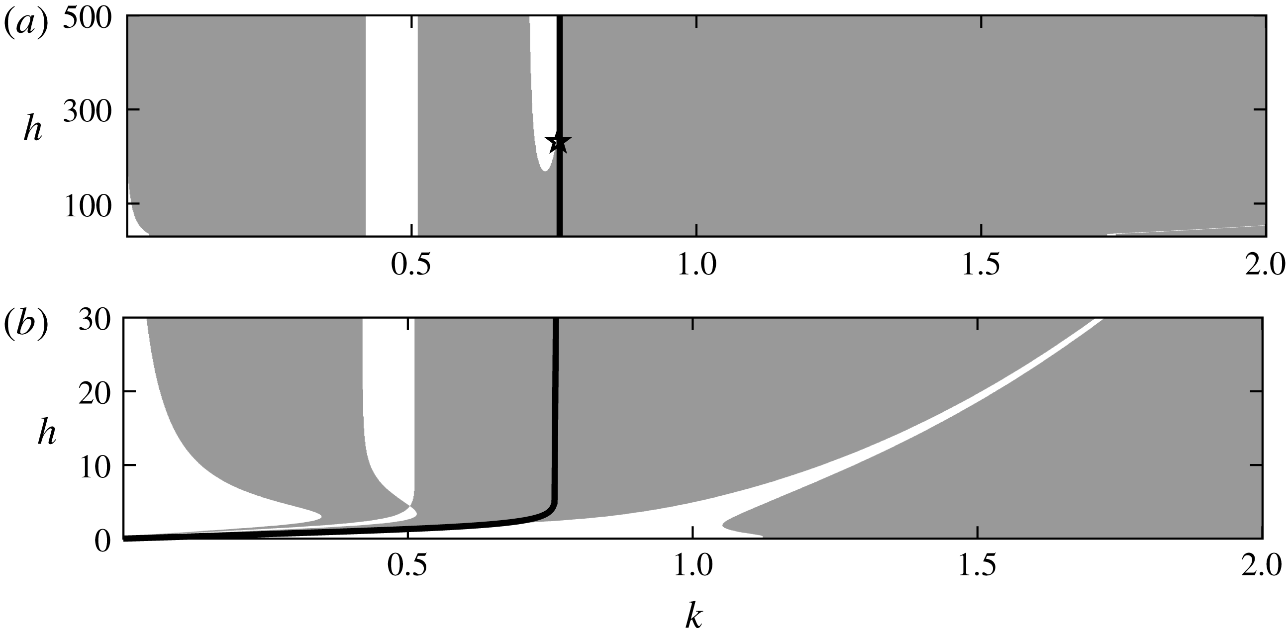
Figure 5. Modulational instability diagrams for hydroelastic waves with no vorticity for
 $30<h<500$
(a) and
$30<h<500$
(a) and
 $h<30$
(b). The stable regions are in white and the unstable are in grey. The thick black curve represents the wavenumbers corresponding to the phase speed minimum at which wavepacket solitary waves bifurcate. The pentagram with the coordinate
$h<30$
(b). The stable regions are in white and the unstable are in grey. The thick black curve represents the wavenumbers corresponding to the phase speed minimum at which wavepacket solitary waves bifurcate. The pentagram with the coordinate
 $(0.7598,233)$
on the thick black curve indicates the location of a stability exchange.
$(0.7598,233)$
on the thick black curve indicates the location of a stability exchange.
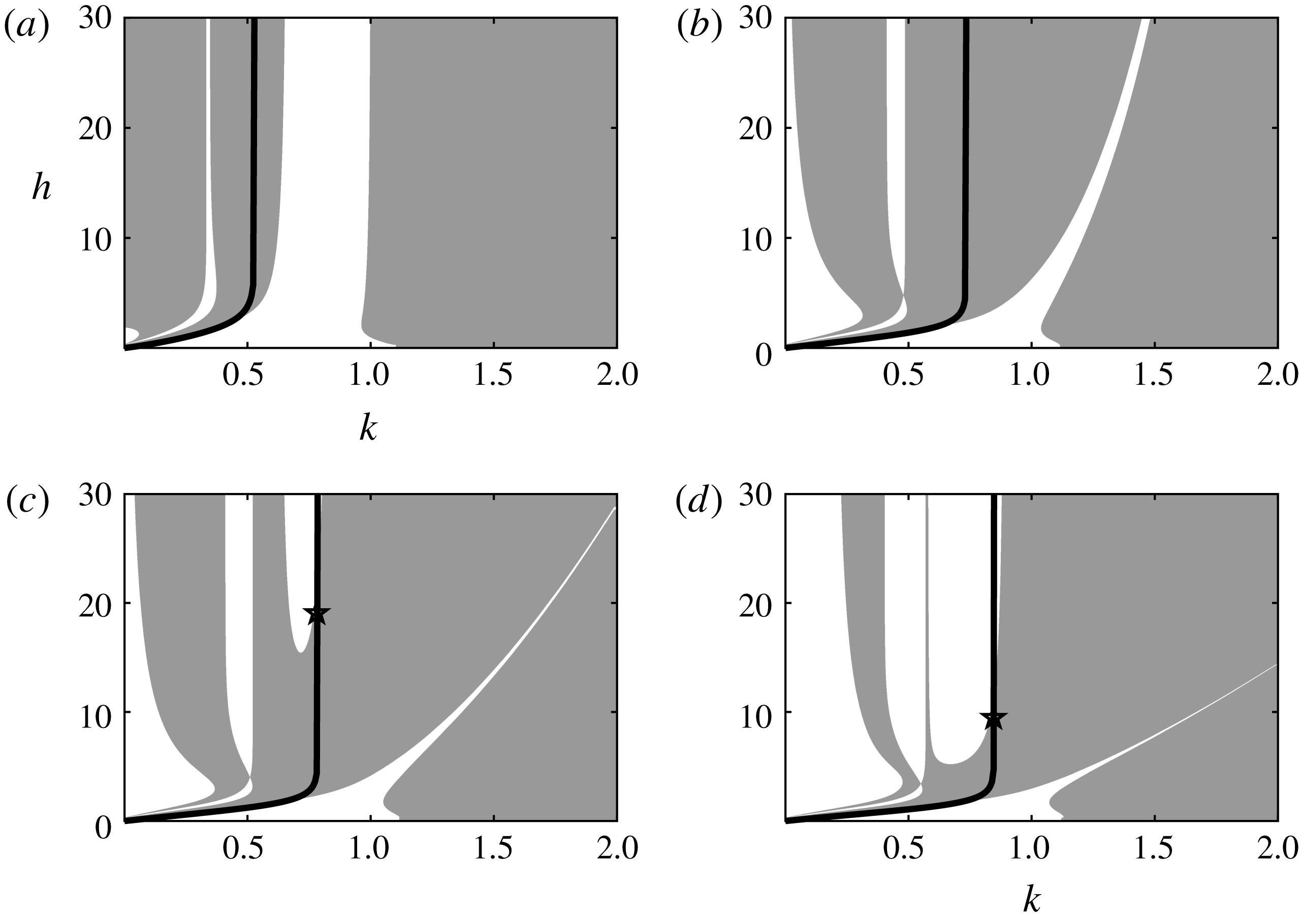
Figure 6. Modulational instability diagram for hydroelastic waves when
 $h<30$
with (a)
$h<30$
with (a)
 $\unicode[STIX]{x1D6FA}_{0}=-1$
, (b)
$\unicode[STIX]{x1D6FA}_{0}=-1$
, (b)
 $\unicode[STIX]{x1D6FA}_{0}=-0.1$
, (c)
$\unicode[STIX]{x1D6FA}_{0}=-0.1$
, (c)
 $\unicode[STIX]{x1D6FA}_{0}=0.1$
and (d)
$\unicode[STIX]{x1D6FA}_{0}=0.1$
and (d)
 $\unicode[STIX]{x1D6FA}_{0}=0.35$
. The stable regions are in white and the unstable are in grey. The thick black curves represent the wavenumbers corresponding to the phase speed minimum at which wavepacket solitary waves bifurcate. Stability exchanges take place at
$\unicode[STIX]{x1D6FA}_{0}=0.35$
. The stable regions are in white and the unstable are in grey. The thick black curves represent the wavenumbers corresponding to the phase speed minimum at which wavepacket solitary waves bifurcate. Stability exchanges take place at
 $(0.785,19.17)$
in (b) and at
$(0.785,19.17)$
in (b) and at
 $(0.8473,9.544)$
in (d).
$(0.8473,9.544)$
in (d).
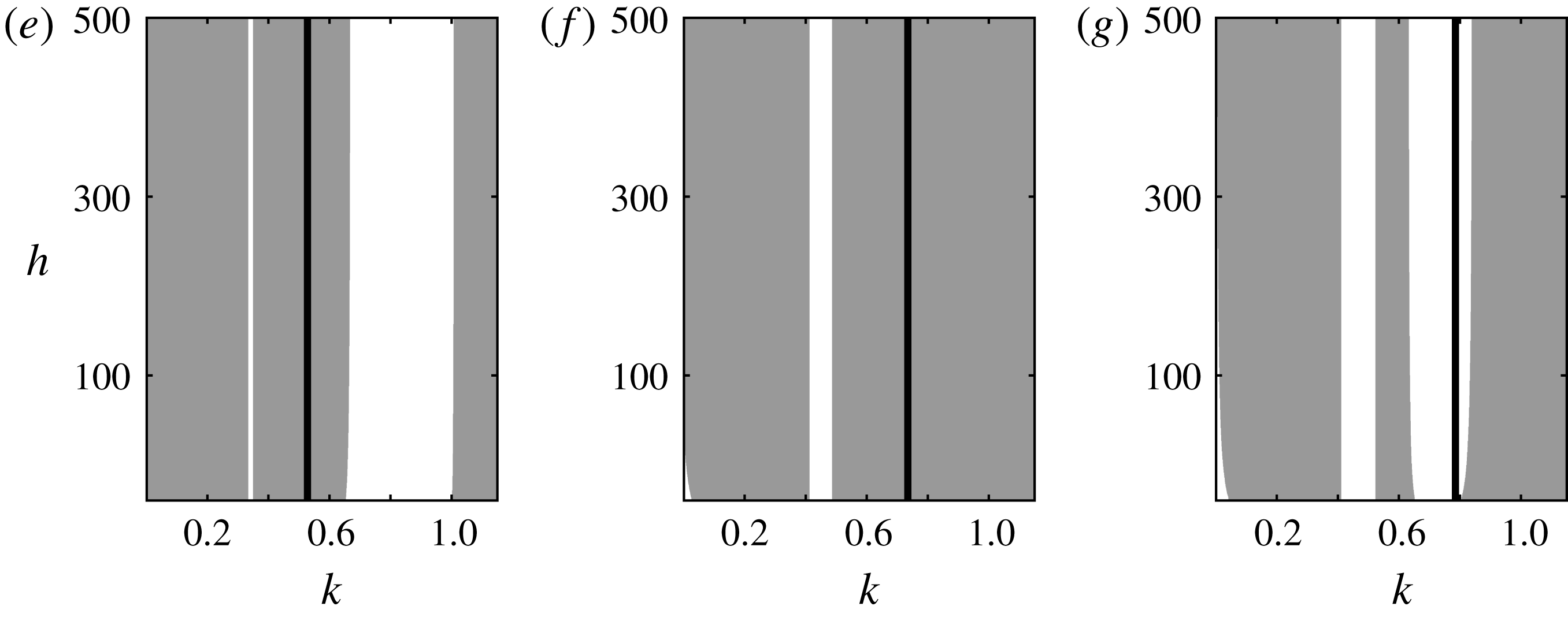
Figure 7. Modulational instability diagrams for hydroelastic waves when
 $30<h<500$
with (e)
$30<h<500$
with (e)
 $\unicode[STIX]{x1D6FA}_{0}=-1$
, (f)
$\unicode[STIX]{x1D6FA}_{0}=-1$
, (f)
 $\unicode[STIX]{x1D6FA}_{0}=-0.1$
, (g)
$\unicode[STIX]{x1D6FA}_{0}=-0.1$
, (g)
 $\unicode[STIX]{x1D6FA}_{0}=0.1$
. The stable regions are in white and the unstable are in grey. The thick black curves represent the wavenumbers corresponding to the phase speed minimum at which wavepacket solitary waves bifurcate.
$\unicode[STIX]{x1D6FA}_{0}=0.1$
. The stable regions are in white and the unstable are in grey. The thick black curves represent the wavenumbers corresponding to the phase speed minimum at which wavepacket solitary waves bifurcate.
In the subsequent sections, we perform numerical simulations in the full Euler equations (2.9) to compute wavepacket solitary waves bifurcation from the thick black curves, and classify the bifurcation mechanisms based on the vor-NLS, as well as examining the time evolution of the modulational instability of quasi-monochromatic wavetrains and the Wilton solutions where the vor-NLS becomes invalid as the second harmonic resonance takes place.
5 Numerical scheme
Numerical simulations for both steady and time-dependent solutions to the constant-vorticity Euler equations can be achieved efficiently by employing a conformal mapping method, which was pioneered for potential flow by Dyachenko et al. (Reference Dyachenko, Kuznetsov, Spectorm and Zakharov1996a
) for deep water, generalised to finite depth in Dynacenko et al. (Reference Dyachenko, Zakharov and Kuznetsov1996b
) (see also Choi & Camassa Reference Choi and Camassa1999) and adapted to constant vorticity cases in Choi (Reference Choi2009). The core idea of this numerical method is to transform the fluid domain onto a fixed simple geometry, e.g. a uniform strip of thickness
 $\bar{h}$
in the new
$\bar{h}$
in the new
 $\unicode[STIX]{x1D709}$
–
$\unicode[STIX]{x1D709}$
–
 $\unicode[STIX]{x1D701}$
plane, where the free boundary is mapped to
$\unicode[STIX]{x1D701}$
plane, where the free boundary is mapped to
 $\unicode[STIX]{x1D701}=0$
. Following Choi & Camassa (Reference Choi and Camassa1999), the difference between
$\unicode[STIX]{x1D701}=0$
. Following Choi & Camassa (Reference Choi and Camassa1999), the difference between
 $h$
and
$h$
and
 $\bar{h}$
is the mean value of the free-surface elevation in the transformed plane, namely,
$\bar{h}$
is the mean value of the free-surface elevation in the transformed plane, namely,
 $$\begin{eqnarray}\displaystyle \bar{h}(t)=h+\frac{1}{L}\int _{-L/2}^{L/2}\,\unicode[STIX]{x1D702}(\unicode[STIX]{x1D709},t)\,\text{d}\unicode[STIX]{x1D709}, & & \displaystyle\end{eqnarray}$$
where
 $L$
is the wavelength. Variables on the upper surface in the transformed plane are defined by
$L$
is the wavelength. Variables on the upper surface in the transformed plane are defined by
 $$\begin{eqnarray}X(\unicode[STIX]{x1D709},t)\triangleq x(\unicode[STIX]{x1D709},0,t),\quad Y(\unicode[STIX]{x1D709},t)\triangleq y(\unicode[STIX]{x1D709},0,t).\end{eqnarray}$$
Calculations similar to those presented in Choi (Reference Choi2009) result in the following surface Euler equations completely describing the evolution
 $$\begin{eqnarray}\displaystyle \left.\begin{array}{@{}c@{}}\displaystyle X_{\unicode[STIX]{x1D709}}=1-{\mathcal{T}}\left[Y_{\unicode[STIX]{x1D709}}\right],\quad \unicode[STIX]{x1D6F7}_{\unicode[STIX]{x1D709}}=-{\mathcal{T}}\left[\unicode[STIX]{x1D6F9}_{\unicode[STIX]{x1D709}}\right],\\ \displaystyle Y_{t}=Y_{\unicode[STIX]{x1D709}}{\mathcal{T}}\left[\frac{\unicode[STIX]{x1D6F9}_{\unicode[STIX]{x1D709}}-\unicode[STIX]{x1D6FA}_{0}YY_{\unicode[STIX]{x1D709}}}{J}\right]-X_{\unicode[STIX]{x1D709}}\left(\frac{\unicode[STIX]{x1D6F9}_{\unicode[STIX]{x1D709}}-\unicode[STIX]{x1D6FA}_{0}YY_{\unicode[STIX]{x1D709}}}{J}\right),\\ \displaystyle \unicode[STIX]{x1D6F7}_{t}=\frac{\unicode[STIX]{x1D6F9}_{\unicode[STIX]{x1D709}}^{2}-\unicode[STIX]{x1D6F7}_{\unicode[STIX]{x1D709}}^{2}}{2J}-Y-{\mathcal{M}}-\unicode[STIX]{x1D6FA}_{0}\left(\unicode[STIX]{x1D6F9}-\frac{YX_{\unicode[STIX]{x1D709}}\unicode[STIX]{x1D6F7}_{\unicode[STIX]{x1D709}}}{J}\right)+\unicode[STIX]{x1D6F7}_{\unicode[STIX]{x1D709}}{\mathcal{T}}\left[\frac{\unicode[STIX]{x1D6F9}_{\unicode[STIX]{x1D709}}-\unicode[STIX]{x1D6FA}_{0}YY_{\unicode[STIX]{x1D709}}}{J}\right],\end{array}\right\} & & \displaystyle\end{eqnarray}$$
where
 ${\mathcal{M}}$
is the pressure exerted by the elastic sheet in the transformed plane and takes the form of
${\mathcal{M}}$
is the pressure exerted by the elastic sheet in the transformed plane and takes the form of
 $$\begin{eqnarray}\displaystyle {\mathcal{M}}=\frac{1}{2}\left[\frac{\unicode[STIX]{x1D705}_{\unicode[STIX]{x1D709}\unicode[STIX]{x1D709}}}{J}+\left(\frac{\unicode[STIX]{x1D705}_{\unicode[STIX]{x1D709}}}{J}\right)_{\unicode[STIX]{x1D709}}+\unicode[STIX]{x1D705}^{3}\right]. & & \displaystyle\end{eqnarray}$$
Here,
 $J\triangleq X_{\unicode[STIX]{x1D709}}^{2}+Y_{\unicode[STIX]{x1D709}}^{2}$
is the Jacobian of the map, and the curvature
$J\triangleq X_{\unicode[STIX]{x1D709}}^{2}+Y_{\unicode[STIX]{x1D709}}^{2}$
is the Jacobian of the map, and the curvature
 $\unicode[STIX]{x1D705}$
is given by
$\unicode[STIX]{x1D705}$
is given by
 $$\begin{eqnarray}\displaystyle \unicode[STIX]{x1D705}=\frac{Y_{\unicode[STIX]{x1D709}\unicode[STIX]{x1D709}}X_{\unicode[STIX]{x1D709}}-X_{\unicode[STIX]{x1D709}\unicode[STIX]{x1D709}}Y_{\unicode[STIX]{x1D709}}}{J^{3/2}}. & & \displaystyle\end{eqnarray}$$
The pseudo-differential operator
 ${\mathcal{T}}$
is defined by
${\mathcal{T}}$
is defined by
 $$\begin{eqnarray}\displaystyle {\mathcal{T}}[f]=\frac{1}{2\bar{h}}\int f(\unicode[STIX]{x1D709}^{\prime })\coth \left[\frac{\unicode[STIX]{x03C0}}{2\bar{h}}(\unicode[STIX]{x1D709}^{\prime }-\unicode[STIX]{x1D709})\right]\,\text{d}\unicode[STIX]{x1D709}^{\prime }. & & \displaystyle\end{eqnarray}$$
In the limit of deep water (
 $\bar{h}\rightarrow \infty$
),
$\bar{h}\rightarrow \infty$
),
 ${\mathcal{T}}$
reduces to the Hilbert transform. For travelling waves translating at a constant velocity
${\mathcal{T}}$
reduces to the Hilbert transform. For travelling waves translating at a constant velocity
 $c$
, the surface Euler equations can be reduced to
$c$
, the surface Euler equations can be reduced to
 $$\begin{eqnarray}\displaystyle & \displaystyle \unicode[STIX]{x1D6F9}=cY+\frac{\unicode[STIX]{x1D6FA}_{0}}{2}Y^{2}, & \displaystyle\end{eqnarray}$$
 $$\begin{eqnarray}\displaystyle & \displaystyle \frac{1}{2J}(c+\unicode[STIX]{x1D6FA}_{0}YX_{\unicode[STIX]{x1D709}}+\unicode[STIX]{x1D6FA}_{0}{\mathcal{T}}[YY_{\unicode[STIX]{x1D709}}])^{2}+B+Y+\frac{1}{2}\left[\frac{\unicode[STIX]{x1D705}_{\unicode[STIX]{x1D709}\unicode[STIX]{x1D709}}}{J}+\left(\frac{\unicode[STIX]{x1D705}_{\unicode[STIX]{x1D709}}}{J}\right)_{\unicode[STIX]{x1D709}}+\unicode[STIX]{x1D705}^{3}\right]=0, & \displaystyle\end{eqnarray}$$
where
 $B$
is the Bernoulli constant (
$B$
is the Bernoulli constant (
 $B=-c^{2}/2$
for solitary waves). Solitary waves are approximated by long periodic waves allowing for efficient computations using the fast Fourier transform. The wave amplitude in periodic and solitary wave cases is defined by
$B=-c^{2}/2$
for solitary waves). Solitary waves are approximated by long periodic waves allowing for efficient computations using the fast Fourier transform. The wave amplitude in periodic and solitary wave cases is defined by
 $$\begin{eqnarray}\displaystyle a={\textstyle \frac{1}{2}}\left(\max _{\unicode[STIX]{x1D709}\in \mathbb{R}}\,Y-\min _{\unicode[STIX]{x1D709}\in \mathbb{R}}\,Y\right). & & \displaystyle\end{eqnarray}$$
We confine ourselves to symmetric steady travelling-wave solutions, which can be written in the form of Fourier series as
 $$\begin{eqnarray}\displaystyle Y=\mathop{\sum }_{n=-N}^{N}a_{n}\text{e}^{\text{i}2\unicode[STIX]{x03C0}n\unicode[STIX]{x1D709}/L},\quad a_{0}=0, & & \displaystyle\end{eqnarray}$$
where the coefficients
 $a_{n}=a_{-n}$
are the real unknowns to be solved by Newton’s method. We introduce
$a_{n}=a_{-n}$
are the real unknowns to be solved by Newton’s method. We introduce
 $N$
collocation points uniformly distributed along the
$N$
collocation points uniformly distributed along the
 $\unicode[STIX]{x1D709}$
-axis, which provides discrete algebraic equations by projecting (5.8) onto each element of the basis
$\unicode[STIX]{x1D709}$
-axis, which provides discrete algebraic equations by projecting (5.8) onto each element of the basis
 $\text{e}^{\text{i}2\unicode[STIX]{x03C0}n\unicode[STIX]{x1D709}/L}$
. All derivatives and pseudo-differential operators are calculated via Fourier multipliers, making the programme efficient and accurate, while the nonlinear terms are computed in real space;
$\text{e}^{\text{i}2\unicode[STIX]{x03C0}n\unicode[STIX]{x1D709}/L}$
. All derivatives and pseudo-differential operators are calculated via Fourier multipliers, making the programme efficient and accurate, while the nonlinear terms are computed in real space;
 $[-L/2,L/2]$
is the domain of computation, which is taken to be sufficiently large for solitary waves so that a further increase in
$[-L/2,L/2]$
is the domain of computation, which is taken to be sufficiently large for solitary waves so that a further increase in
 $L$
does not change the solution to numerical accuracy.
$L$
does not change the solution to numerical accuracy.
6 Numerical results
6.1 Solitary waves
In the weakly nonlinear theory, the existence of wavepacket solitary waves requires two conditions: a non-dispersive point in the dispersion relation where the group velocity
 $c_{g}$
equals the phase velocity
$c_{g}$
equals the phase velocity
 $c_{p}$
and a focussing NLS at this particular point, therefore the envelope can modulate carrier wave into a locally confined travelling solution. The general solution of bright soliton for (4.1) takes the form
$c_{p}$
and a focussing NLS at this particular point, therefore the envelope can modulate carrier wave into a locally confined travelling solution. The general solution of bright soliton for (4.1) takes the form
 $$\begin{eqnarray}\displaystyle A(X,\unicode[STIX]{x1D70F})=\sqrt{\frac{2C}{\unicode[STIX]{x1D6FE}}}\operatorname{sech}\left(\unicode[STIX]{x1D716}\sqrt{\frac{C}{\unicode[STIX]{x1D706}}}X\right)\text{e}^{\text{i}C\unicode[STIX]{x1D70F}}, & & \displaystyle\end{eqnarray}$$
where
 $C$
is a positive constant. It follows that
$C$
is a positive constant. It follows that
 $$\begin{eqnarray}\displaystyle \unicode[STIX]{x1D702}(x,t)\approx 2\unicode[STIX]{x1D716}\sqrt{\frac{2C}{\unicode[STIX]{x1D6FE}}}\operatorname{sech}\left(\unicode[STIX]{x1D716}\sqrt{\frac{C}{\unicode[STIX]{x1D706}}}\left(x-c_{g}t\right)\right)\cos \left[k\left(x-c_{p}t+\frac{\unicode[STIX]{x1D716}^{2}C}{k}t\right)+\unicode[STIX]{x1D703}_{0}\right], & & \displaystyle\end{eqnarray}$$
where
 $\unicode[STIX]{x1D703}_{0}$
is the relative phase between the carrier wave and the envelope, and the carrier and envelope speeds can be made to match exactly by perturbing the carrier wavenumber
$\unicode[STIX]{x1D703}_{0}$
is the relative phase between the carrier wave and the envelope, and the carrier and envelope speeds can be made to match exactly by perturbing the carrier wavenumber
 $k$
. The phase
$k$
. The phase
 $\unicode[STIX]{x1D703}_{0}$
, while it is a free parameter within the NLS framework, should be taken as
$\unicode[STIX]{x1D703}_{0}$
, while it is a free parameter within the NLS framework, should be taken as
 $0$
or
$0$
or
 $\unicode[STIX]{x03C0}$
(Akers & Milewski Reference Akers and Milewski2009). This is a good approximation for wavepacket solitary waves in the primitive equations and can serve as the initial guess for Newton’s method. In the absence of vorticity, the NLS for hydroelastic waves changes type at a critical value of depth
$\unicode[STIX]{x03C0}$
(Akers & Milewski Reference Akers and Milewski2009). This is a good approximation for wavepacket solitary waves in the primitive equations and can serve as the initial guess for Newton’s method. In the absence of vorticity, the NLS for hydroelastic waves changes type at a critical value of depth
 $h_{c}=233$
. More generally,
$h_{c}=233$
. More generally,
 $h_{c}$
can be presented as a function in
$h_{c}$
can be presented as a function in
 $\unicode[STIX]{x1D6FA}_{0}$
(see figure 8). If
$\unicode[STIX]{x1D6FA}_{0}$
(see figure 8). If
 $h>h_{c}$
, the NLS is defocussing otherwise focussing. Nevertheless, even in the defocussing situation, the weakly nonlinear theory does not deny the existence of wavepacket solitary waves in the fully nonlinear equations. There is a vertical asymptote near
$h>h_{c}$
, the NLS is defocussing otherwise focussing. Nevertheless, even in the defocussing situation, the weakly nonlinear theory does not deny the existence of wavepacket solitary waves in the fully nonlinear equations. There is a vertical asymptote near
 $\unicode[STIX]{x1D6FA}_{0}=-0.005$
where
$\unicode[STIX]{x1D6FA}_{0}=-0.005$
where
 $h_{c}$
tends to infinity. As shown by Milewski et al. (Reference Milewski, Vanden-Broeck and Wang2011), Guyenne & Părău (Reference Guyenne and Părău2012), Gao et al. (Reference Gao, Wang and Vanden-Broeck2016), hydroelastic solitary waves do exist in deep water at finite amplitude where the weakly nonlinear theory does not apply. In this regime, small-amplitude ‘dark’ solitary waves can also be found (Milewski et al.
Reference Milewski, Vanden-Broeck and Wang2013).
$h_{c}$
tends to infinity. As shown by Milewski et al. (Reference Milewski, Vanden-Broeck and Wang2011), Guyenne & Părău (Reference Guyenne and Părău2012), Gao et al. (Reference Gao, Wang and Vanden-Broeck2016), hydroelastic solitary waves do exist in deep water at finite amplitude where the weakly nonlinear theory does not apply. In this regime, small-amplitude ‘dark’ solitary waves can also be found (Milewski et al.
Reference Milewski, Vanden-Broeck and Wang2013).
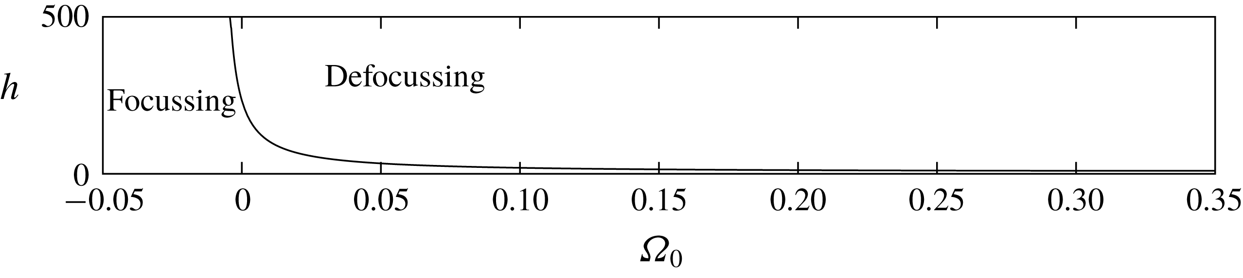
Figure 8. Curve
 $h=h_{c}$
versus
$h=h_{c}$
versus
 $\unicode[STIX]{x1D6FA}_{0}$
.
$\unicode[STIX]{x1D6FA}_{0}$
.
Table 1. The values of the coefficients in the vor-NLS, the minimum phase speeds and the associated wavenumber for different
 $\unicode[STIX]{x1D6FA}_{0}$
.
$\unicode[STIX]{x1D6FA}_{0}$
.

Positive vorticity can decrease the depth at which the vor-NLS coefficient changes sign (see figures 6
c,d and 7
g). As an example, coefficients of (4.1) for different values of
 $\unicode[STIX]{x1D6FA}_{0}$
are listed in table 1. We start with
$\unicode[STIX]{x1D6FA}_{0}$
are listed in table 1. We start with
 $h=500$
(
$h=500$
(
 ${>}h_{c}$
), the case that the associated NLS is defocussing at the minimum of the phase speed (denoted by
${>}h_{c}$
), the case that the associated NLS is defocussing at the minimum of the phase speed (denoted by
 $c_{min}$
) in the absence of vorticity. As listed in table 1, a negative vorticity may change the type of the NLS. As a result, wavepacket solitary waves may bifurcate from zero amplitude at
$c_{min}$
) in the absence of vorticity. As listed in table 1, a negative vorticity may change the type of the NLS. As a result, wavepacket solitary waves may bifurcate from zero amplitude at
 $c_{min}$
with a sufficiently large
$c_{min}$
with a sufficiently large
 $|\unicode[STIX]{x1D6FA}_{0}|$
. This feature is confirmed by our numerical results for
$|\unicode[STIX]{x1D6FA}_{0}|$
. This feature is confirmed by our numerical results for
 $\unicode[STIX]{x1D6FA}_{0}=-1$
as shown in the speed–amplitude bifurcation diagram (figure 9
a). If we assume the phase speed attains its minimum at the wavenumber
$\unicode[STIX]{x1D6FA}_{0}=-1$
as shown in the speed–amplitude bifurcation diagram (figure 9
a). If we assume the phase speed attains its minimum at the wavenumber
 $k_{c}$
, then the leading order of the NLS prediction for amplitude reads
$k_{c}$
, then the leading order of the NLS prediction for amplitude reads
 $$\begin{eqnarray}\displaystyle \Vert \unicode[STIX]{x1D702}\Vert _{\infty }\approx 2\unicode[STIX]{x1D716}\sqrt{\frac{2C}{\unicode[STIX]{x1D6FE}}}\approx (c_{min}-c)^{1/2}\sqrt{\frac{8k_{c}}{\unicode[STIX]{x1D6FE}}}. & & \displaystyle\end{eqnarray}$$
This relation is also sketched in figure 9 (dot-dashed line), which matches the nonlinear results well in the vicinity of the minimum phase speed. It is noted that the prediction for the elevation solitary waves can be improved by including a second harmonic correction term which, on the contrary, generally worsens the prediction for depression waves as explained in Wang & Milewski (Reference Wang and Milewski2012) . Numerical computations for
 $\unicode[STIX]{x1D6FA}_{0}=0.1$
are performed and presented in figure 9(
$\unicode[STIX]{x1D6FA}_{0}=0.1$
are performed and presented in figure 9(
 $b$
). This speed–amplitude diagram illustrates that the solitary waves bifurcate from non-zero amplitude. That is because the vor-NLS is of defocussing type under these parameters and hence small-amplitude wavepacket solitary waves are ruled out.
$b$
). This speed–amplitude diagram illustrates that the solitary waves bifurcate from non-zero amplitude. That is because the vor-NLS is of defocussing type under these parameters and hence small-amplitude wavepacket solitary waves are ruled out.
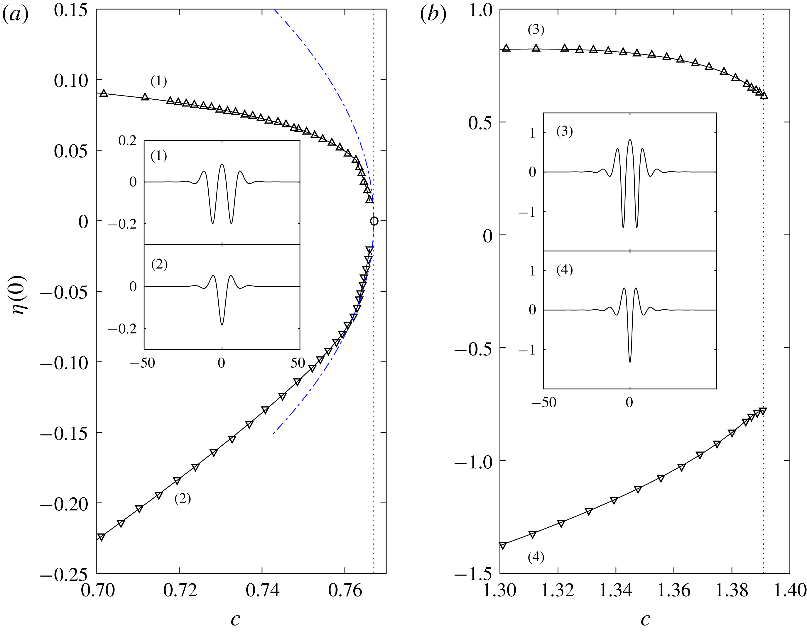
Figure 9. Local bifurcation diagrams of hydroelastic solitary waves for
 $h=500$
. The upward-pointing and downward-pointing triangles are for the elevation and depression waves respectively. The minimum phase speeds are marked as the dotted lines. (a)
$h=500$
. The upward-pointing and downward-pointing triangles are for the elevation and depression waves respectively. The minimum phase speeds are marked as the dotted lines. (a)
 $\unicode[STIX]{x1D6FA}_{0}=-1$
: the associated NLS is of focussing type when, and its leading-order prediction is sketched as the dot-dashed curve. (b)
$\unicode[STIX]{x1D6FA}_{0}=-1$
: the associated NLS is of focussing type when, and its leading-order prediction is sketched as the dot-dashed curve. (b)
 $\unicode[STIX]{x1D6FA}_{0}=0.1$
: the associated NLS is of defocussing type, and the solitary waves bifurcate at non-zero amplitude. Typical wave profiles are presented in the physical space in both panels.
$\unicode[STIX]{x1D6FA}_{0}=0.1$
: the associated NLS is of defocussing type, and the solitary waves bifurcate at non-zero amplitude. Typical wave profiles are presented in the physical space in both panels.
We then focus on the case of small depth (
 $h=10<h_{c}$
). The vor-NLS is focussing without vorticity, but a positive vorticity can change it to defocussing, as demonstrated in table 1. This is again confirmed by our numerical simulations as shown in figure 10(b), which illustrates that, near
$h=10<h_{c}$
). The vor-NLS is focussing without vorticity, but a positive vorticity can change it to defocussing, as demonstrated in table 1. This is again confirmed by our numerical simulations as shown in figure 10(b), which illustrates that, near
 $c_{min}$
, solitary waves can only exist at finite amplitude. The case for negative vorticity
$c_{min}$
, solitary waves can only exist at finite amplitude. The case for negative vorticity
 $\unicode[STIX]{x1D6FA}_{0}=-1$
(corresponding to focussing NLS) is also investigated. We present the detailed local bifurcation structure in figure 10(a) together with the leading-order NLS prediction. The agreement between the nonlinear results and the theoretical prediction is good especially for depression waves. Typical wave profiles featuring oscillatory decaying tails are also shown for both elevation and depression branches. The computations shown in figures 9 and 10 are carried out with
$\unicode[STIX]{x1D6FA}_{0}=-1$
(corresponding to focussing NLS) is also investigated. We present the detailed local bifurcation structure in figure 10(a) together with the leading-order NLS prediction. The agreement between the nonlinear results and the theoretical prediction is good especially for depression waves. Typical wave profiles featuring oscillatory decaying tails are also shown for both elevation and depression branches. The computations shown in figures 9 and 10 are carried out with
 $L=200$
and
$L=200$
and
 $N=4096$
. The maximal strains in the ice are calculated from the numerical results with dimensions by using the physical parameters of sea ice. They are at the level of
$N=4096$
. The maximal strains in the ice are calculated from the numerical results with dimensions by using the physical parameters of sea ice. They are at the level of
 $10^{-6}$
which is way below the critical value, i.e. no ice breaking can take place.
$10^{-6}$
which is way below the critical value, i.e. no ice breaking can take place.
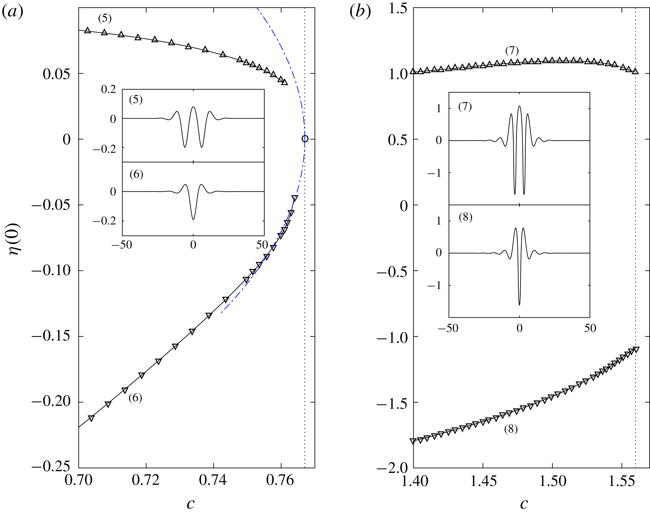
Figure 10. Local bifurcation diagrams of hydroelastic solitary waves for
 $h=10$
. The upward-pointing and downward-pointing triangles are for the elevation and depression waves respectively. The minimum phase speeds are marked as the dotted lines. (a)
$h=10$
. The upward-pointing and downward-pointing triangles are for the elevation and depression waves respectively. The minimum phase speeds are marked as the dotted lines. (a)
 $\unicode[STIX]{x1D6FA}_{0}=-1$
: the associated NLS is of focussing type, and its leading-order prediction is sketched as the dot-dashed curve. (b)
$\unicode[STIX]{x1D6FA}_{0}=-1$
: the associated NLS is of focussing type, and its leading-order prediction is sketched as the dot-dashed curve. (b)
 $\unicode[STIX]{x1D6FA}_{0}=0.35$
: the associated NLS is of defocussing type, and the solitary waves bifurcate at non-zero amplitude. Typical wave profiles are presented in the physical space in both panels.
$\unicode[STIX]{x1D6FA}_{0}=0.35$
: the associated NLS is of defocussing type, and the solitary waves bifurcate at non-zero amplitude. Typical wave profiles are presented in the physical space in both panels.
6.2 Time-dependent simulations
It is well acknowledged (also shown in § 4) that a focussing NLS predicts the modulational instability, which is also called the Benjamin–Feir (BF) instability in water waves (Benjamin & Feir Reference Benjamin and Feir1967). Choi (Reference Choi2009) investigated the BF instability for pure gravity waves propagating on a linear shear current. Based on the assumptions that the basic shear flow is
 $u_{0}+\unicode[STIX]{x1D6FA}_{0}y$
for
$u_{0}+\unicode[STIX]{x1D6FA}_{0}y$
for
 $-h<y<0$
and a wavetrain propagates at the speed
$-h<y<0$
and a wavetrain propagates at the speed
 $u_{0}$
, the author concluded that positive
$u_{0}$
, the author concluded that positive
 $\unicode[STIX]{x1D6FA}_{0}$
enhances the BF instability while the opposite is true for the negative
$\unicode[STIX]{x1D6FA}_{0}$
enhances the BF instability while the opposite is true for the negative
 $\unicode[STIX]{x1D6FA}_{0}$
. In the subsequent numerical experiments, we perform fully nonlinear simulations to examine the modulational instability for hydroelastic waves with linear shear currents. The equations (5.3) are simulated with the initial condition, as in Tanaka (Reference Tanaka1990),
$\unicode[STIX]{x1D6FA}_{0}$
. In the subsequent numerical experiments, we perform fully nonlinear simulations to examine the modulational instability for hydroelastic waves with linear shear currents. The equations (5.3) are simulated with the initial condition, as in Tanaka (Reference Tanaka1990),
 $$\begin{eqnarray}\unicode[STIX]{x1D702}(x,0)=\left[1+\unicode[STIX]{x1D6FC}\cos K\left(x-\frac{\unicode[STIX]{x1D6FD}\unicode[STIX]{x1D706}}{2\unicode[STIX]{x03C0}}\right)\right]\unicode[STIX]{x1D702}_{0}(x),\end{eqnarray}$$
where
 $\unicode[STIX]{x1D702}_{0}$
is a Stokes wave (i.e. a nonlinear solution to the Euler equations),
$\unicode[STIX]{x1D702}_{0}$
is a Stokes wave (i.e. a nonlinear solution to the Euler equations),
 $\unicode[STIX]{x1D6FD}\in [0,2\unicode[STIX]{x03C0})$
is a relative phase between the carrier and the envelope. The modulational wavenumber
$\unicode[STIX]{x1D6FD}\in [0,2\unicode[STIX]{x03C0})$
is a relative phase between the carrier and the envelope. The modulational wavenumber
 $K$
is chosen to be
$K$
is chosen to be
 $k/m$
with
$k/m$
with
 $m$
being a positive integer, i.e.
$m$
being a positive integer, i.e.
 $m$
carrier waves in one modulation. We restrict our focus to the case
$m$
carrier waves in one modulation. We restrict our focus to the case
 $h=10$
and perform experiments with different values of the vorticity
$h=10$
and perform experiments with different values of the vorticity
 $\unicode[STIX]{x1D6FA}_{0}$
.
$\unicode[STIX]{x1D6FA}_{0}$
.
6.2.1 NLS regime
The first numerical experiment is performed in the modulational stable regime by using the following parameters:
 $h=10$
,
$h=10$
,
 $\unicode[STIX]{x1D6FA}_{0}=0.35$
,
$\unicode[STIX]{x1D6FA}_{0}=0.35$
,
 $a=0.05$
,
$a=0.05$
,
 $c=1.7560$
,
$c=1.7560$
,
 $l=12$
(we denote
$l=12$
(we denote
 $l$
by the wavelength of the carrier wave
$l$
by the wavelength of the carrier wave
 $\unicode[STIX]{x1D702}_{0}$
),
$\unicode[STIX]{x1D702}_{0}$
),
 $m=16$
,
$m=16$
,
 $\unicode[STIX]{x1D6FD}=0$
,
$\unicode[STIX]{x1D6FD}=0$
,
 $\unicode[STIX]{x1D6FC}=0.1$
,
$\unicode[STIX]{x1D6FC}=0.1$
,
 $L=192$
,
$L=192$
,
 $K=2\unicode[STIX]{x03C0}/L$
,
$K=2\unicode[STIX]{x03C0}/L$
,
 $N=2048$
and
$N=2048$
and
 $\text{d}t=0.001$
. As shown in figure 11(a,d), the wave keeps travelling in a moving frame of reference without losing its sinusoidal structure. The Fourier spectrum barely changes as time evolves, therefore no modulational instability has been detected, as predicted by the vor-NLS. We have computed the time evolution of this wavetrain for many other values of
$\text{d}t=0.001$
. As shown in figure 11(a,d), the wave keeps travelling in a moving frame of reference without losing its sinusoidal structure. The Fourier spectrum barely changes as time evolves, therefore no modulational instability has been detected, as predicted by the vor-NLS. We have computed the time evolution of this wavetrain for many other values of
 $K$
and
$K$
and
 $\unicode[STIX]{x1D6FD}$
, and have obtained qualitatively similar results that confirm the modulational stability predicted by the NLS. We denote the amplification ratio by
$\unicode[STIX]{x1D6FD}$
, and have obtained qualitatively similar results that confirm the modulational stability predicted by the NLS. We denote the amplification ratio by
 $R(t)$
: the ratio of the maximum wave amplitude at time
$R(t)$
: the ratio of the maximum wave amplitude at time
 $t$
divided by
$t$
divided by
 $a$
(see Tanaka Reference Tanaka1990). As can be seen from in figure 11(c), the amplification parameter exhibits oscillatory behaviour of period approximately
$a$
(see Tanaka Reference Tanaka1990). As can be seen from in figure 11(c), the amplification parameter exhibits oscillatory behaviour of period approximately
 $6800$
(the prediction from NLS for this modulation–demodulation is
$6800$
(the prediction from NLS for this modulation–demodulation is
 $T_{m}=6558$
).
$T_{m}=6558$
).
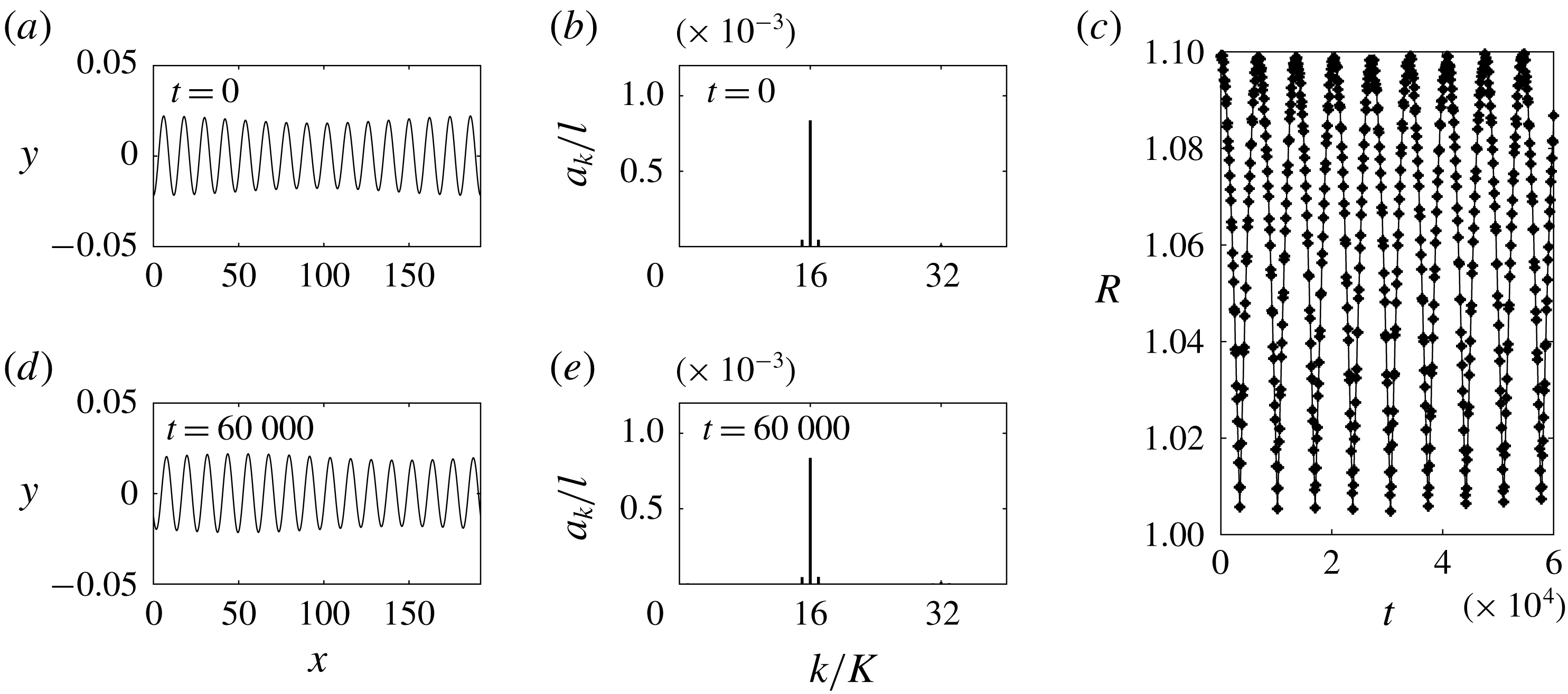
Figure 11. (a,d) Time evolution of a Stokes wave with
 $h=10$
,
$h=10$
,
 $\unicode[STIX]{x1D6FA}_{0}=0.35$
,
$\unicode[STIX]{x1D6FA}_{0}=0.35$
,
 $a=0.02$
,
$a=0.02$
,
 $c=1.7560$
,
$c=1.7560$
,
 $l=12$
,
$l=12$
,
 $L=192$
and
$L=192$
and
 $K=0.0327$
which is initially given a modulational perturbation. A frame of reference moving with the undisturbed wave is chosen. The snapshots are taken at
$K=0.0327$
which is initially given a modulational perturbation. A frame of reference moving with the undisturbed wave is chosen. The snapshots are taken at
 $t=0$
and
$t=0$
and
 $60\,000$
. (b,e) Fourier spectrum of the wave at
$60\,000$
. (b,e) Fourier spectrum of the wave at
 $t=0$
and
$t=0$
and
 $60\,000$
. (c) Graph of
$60\,000$
. (c) Graph of
 $R$
versus
$R$
versus
 $t$
.
$t$
.

Figure 12. Time evolution of a Stokes wave, which is initially given a modulational perturbation, with
 $h=10$
,
$h=10$
,
 $\unicode[STIX]{x1D6FA}_{0}=-1$
,
$\unicode[STIX]{x1D6FA}_{0}=-1$
,
 $a=0.02$
,
$a=0.02$
,
 $c=0.7694$
,
$c=0.7694$
,
 $l=10.85$
and
$l=10.85$
and
 $\unicode[STIX]{x1D6FD}=0$
for different values of modulational wavenumber. (a) Graph of
$\unicode[STIX]{x1D6FD}=0$
for different values of modulational wavenumber. (a) Graph of
 $R$
versus
$R$
versus
 $t$
for (○)
$t$
for (○)
 $K=0.0386$
(
$K=0.0386$
(
 $m=15$
), (▵)
$m=15$
), (▵)
 $K=0.0290$
(
$K=0.0290$
(
 $m=20$
), (▿)
$m=20$
), (▿)
 $K=0.0579$
(
$K=0.0579$
(
 $m=10$
) and (♢)
$m=10$
) and (♢)
 $K=0.1158$
(
$K=0.1158$
(
 $m=5$
) for
$m=5$
) for
 $0\leqslant t\leqslant 2000$
. (b) The snapshots of the wave profiles for
$0\leqslant t\leqslant 2000$
. (b) The snapshots of the wave profiles for
 $\unicode[STIX]{x1D6FD}=0$
at
$\unicode[STIX]{x1D6FD}=0$
at
 $t=2000$
in a large domain
$t=2000$
in a large domain
 $[0,651]$
. (c) The corresponding Fourier spectra of the waves at
$[0,651]$
. (c) The corresponding Fourier spectra of the waves at
 $t=2000$
.
$t=2000$
.
The second experiment is made in the unstable regime for a wave travelling at a speed close to
 $c_{min}$
with parameters
$c_{min}$
with parameters
 $h=10$
,
$h=10$
,
 $\unicode[STIX]{x1D6FA}_{0}=-1$
,
$\unicode[STIX]{x1D6FA}_{0}=-1$
,
 $a=0.02$
,
$a=0.02$
,
 $c=0.7694$
,
$c=0.7694$
,
 $l=10.85$
,
$l=10.85$
,
 $\unicode[STIX]{x1D6FC}=0.1$
,
$\unicode[STIX]{x1D6FC}=0.1$
,
 $N=2048$
and
$N=2048$
and
 $\text{d}t=0.001$
, for different values of
$\text{d}t=0.001$
, for different values of
 $K=k/m$
and
$K=k/m$
and
 $L=ml$
with
$L=ml$
with
 $m=5$
,
$m=5$
,
 $10$
,
$10$
,
 $15$
and
$15$
and
 $20$
, in which
$20$
, in which
 $m=15$
is the optimal integer for the maximal growth from (4.10). According to (4.11), the modulational instability is present for
$m=15$
is the optimal integer for the maximal growth from (4.10). According to (4.11), the modulational instability is present for
 $m\geqslant 10$
, which is confirmed by the numerical results. The curve of
$m\geqslant 10$
, which is confirmed by the numerical results. The curve of
 $R$
against
$R$
against
 $t$
is shown in figure 12(a) for shorter times
$t$
is shown in figure 12(a) for shorter times
 $0\leqslant t\leqslant 2000$
alongside the snapshots of the wave profile taken at
$0\leqslant t\leqslant 2000$
alongside the snapshots of the wave profile taken at
 $t=2000$
in (b), and their associated Fourier spectra in (c). Within this time range,
$t=2000$
in (b), and their associated Fourier spectra in (c). Within this time range,
 $R$
exhibits clear monotonic growth for unstable wavenumbers and hence one may compare the values of
$R$
exhibits clear monotonic growth for unstable wavenumbers and hence one may compare the values of
 $R$
for various modulational wavenumbers. Clearly
$R$
for various modulational wavenumbers. Clearly
 $m=15$
grows fastest, which confirms the prediction by the NLS. We continue to compute
$m=15$
grows fastest, which confirms the prediction by the NLS. We continue to compute
 $R$
over a larger time domain
$R$
over a larger time domain
 $[0,8000]$
for
$[0,8000]$
for
 $m=15$
in figure 13. A snapshot of the wave profile at maximum
$m=15$
in figure 13. A snapshot of the wave profile at maximum
 $R$
is depicted on the right of the same figure. Next, computations with various initial phases are carried out. The numerical results are presented in figure 14 where
$R$
is depicted on the right of the same figure. Next, computations with various initial phases are carried out. The numerical results are presented in figure 14 where
 $R$
is plotted against
$R$
is plotted against
 $\unicode[STIX]{x1D6FD}$
at
$\unicode[STIX]{x1D6FD}$
at
 $t=2000$
in the left and, for
$t=2000$
in the left and, for
 $m=15$
, at the maximum amplification
$m=15$
, at the maximum amplification
 $R_{max}$
on the right. The growth over this period and the maximum growth over longer periods exhibit only weak
$R_{max}$
on the right. The growth over this period and the maximum growth over longer periods exhibit only weak
 $\unicode[STIX]{x1D6FD}$
-dependency. There is evidence in the literature that reduced models (Stiassnie & Kroszynski Reference Stiassnie and Kroszynski1982) exhibit specific phase values at which there may be no initial growth in the modulationally unstable case due to a projection of the initial data onto the decaying mode only. While we have not specifically sought to reproduce that, we still see some phase dependence in the amplification
$\unicode[STIX]{x1D6FD}$
-dependency. There is evidence in the literature that reduced models (Stiassnie & Kroszynski Reference Stiassnie and Kroszynski1982) exhibit specific phase values at which there may be no initial growth in the modulationally unstable case due to a projection of the initial data onto the decaying mode only. While we have not specifically sought to reproduce that, we still see some phase dependence in the amplification
 $R(2000)$
. Consistently with Stiassnie & Kroszynski (Reference Stiassnie and Kroszynski1982) this phase dependence varies with
$R(2000)$
. Consistently with Stiassnie & Kroszynski (Reference Stiassnie and Kroszynski1982) this phase dependence varies with
 $m$
.
$m$
.
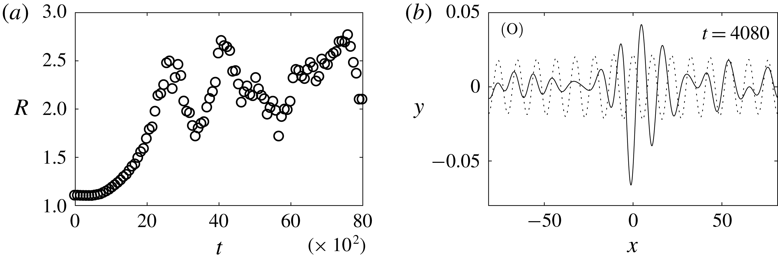
Figure 13. Same numerical experiment as in figure 12. (a) Graph of
 $R$
versus
$R$
versus
 $t$
in a large time domain
$t$
in a large time domain
 $[0,8000]$
for
$[0,8000]$
for
 $K=0.0386$
(
$K=0.0386$
(
 $m=15$
). (b) Snapshot of the associated maximum modulation taken at
$m=15$
). (b) Snapshot of the associated maximum modulation taken at
 $t=4080$
. The initial wave profile is shown by the dotted curve.
$t=4080$
. The initial wave profile is shown by the dotted curve.

Figure 14. Same numerical experiment as in figure 12 with various initial phases. (a) Graph of
 $R$
versus
$R$
versus
 $\unicode[STIX]{x1D6FD}$
at
$\unicode[STIX]{x1D6FD}$
at
 $t=2000$
for (○)
$t=2000$
for (○)
 $K=0.0386$
(
$K=0.0386$
(
 $m=15$
), (▵)
$m=15$
), (▵)
 $K=0.0290$
(
$K=0.0290$
(
 $m=20$
), (▿)
$m=20$
), (▿)
 $K=0.0579$
(
$K=0.0579$
(
 $m=10$
) and (♢)
$m=10$
) and (♢)
 $K=0.1158$
(
$K=0.1158$
(
 $m=5$
). (b) Graph of the maximum amplification
$m=5$
). (b) Graph of the maximum amplification
 $R_{max}$
versus
$R_{max}$
versus
 $\unicode[STIX]{x1D6FD}$
for
$\unicode[STIX]{x1D6FD}$
for
 $K=0.0386$
(
$K=0.0386$
(
 $m=15$
).
$m=15$
).
6.2.2 Highly nonlinear regime
In this subsection, we conduct numerical time-dependent simulations for highly nonlinear waves where the vor-NLS is no longer appropriate.
The first experiment is performed in the stable NLS regime with the same parameters from figure 11 except for a much larger amplitude
 $a=0.5$
(the associated wave speed
$a=0.5$
(the associated wave speed
 $c=2.1273$
). The snapshots and the Fourier spectrum at two different times are shown in figure 15, which indicate that large side-band modes grow in time and the envelope breaks up at some point. This phenomenon is caused by a strong modulational instability of the finite-amplitude wave.
$c=2.1273$
). The snapshots and the Fourier spectrum at two different times are shown in figure 15, which indicate that large side-band modes grow in time and the envelope breaks up at some point. This phenomenon is caused by a strong modulational instability of the finite-amplitude wave.
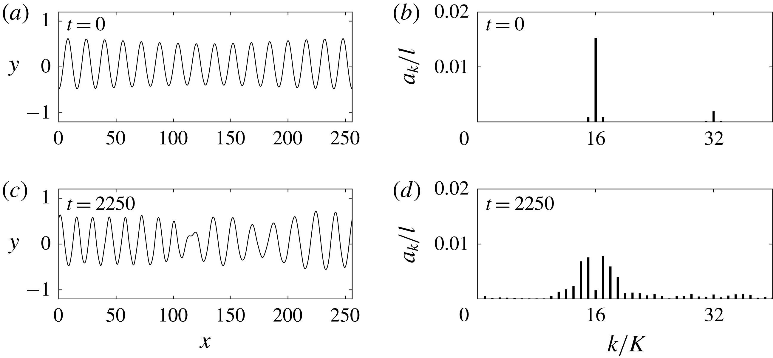
Figure 15. (a,c) Time evolution of a Stokes wave with
 $h=10$
,
$h=10$
,
 $\unicode[STIX]{x1D6FA}_{0}=0.35$
,
$\unicode[STIX]{x1D6FA}_{0}=0.35$
,
 $c=2.1273$
,
$c=2.1273$
,
 $a=0.5$
,
$a=0.5$
,
 $l=16$
,
$l=16$
,
 $L=256$
and
$L=256$
and
 $K=0.0245$
which is initially given a modulational perturbation. The snapshots are taken at
$K=0.0245$
which is initially given a modulational perturbation. The snapshots are taken at
 $t=0$
and
$t=0$
and
 $2250$
. (b,d) Fourier spectrum of the wave at
$2250$
. (b,d) Fourier spectrum of the wave at
 $t=0$
and
$t=0$
and
 $2250$
.
$2250$
.
The second experiment is conducted in the unstable NLS regime on the same carrier wave from figure 12 but with a much larger amplitude
 $a=0.2$
. We select
$a=0.2$
. We select
 $\unicode[STIX]{x1D6FD}=0$
and
$\unicode[STIX]{x1D6FD}=0$
and
 $m=15$
which is associated with the optimal value of
$m=15$
which is associated with the optimal value of
 $K$
. As can be seen from figure 16, the BF modulational instability occurs at first, but this is followed, at a later stage, by a large depression wave structure, which is greater than twice the amplitude of surrounding waves. This feature is different from the BF numerical observations for small-amplitude pure gravity waves, where a significant elevation structure is observed by Choi (Reference Choi2009). (Large water waves arising from modulational instabilities are often given as a mechanism for the generation of ‘rogue waves’ Kharif & Pelinovsky (Reference Kharif and Pelinovsky2003)). A similar computation is performed for a highly nonlinear short wave with
$K$
. As can be seen from figure 16, the BF modulational instability occurs at first, but this is followed, at a later stage, by a large depression wave structure, which is greater than twice the amplitude of surrounding waves. This feature is different from the BF numerical observations for small-amplitude pure gravity waves, where a significant elevation structure is observed by Choi (Reference Choi2009). (Large water waves arising from modulational instabilities are often given as a mechanism for the generation of ‘rogue waves’ Kharif & Pelinovsky (Reference Kharif and Pelinovsky2003)). A similar computation is performed for a highly nonlinear short wave with
 $h=10$
,
$h=10$
,
 $\unicode[STIX]{x1D6FA}_{0}=-1$
,
$\unicode[STIX]{x1D6FA}_{0}=-1$
,
 $c=5.2399$
,
$c=5.2399$
,
 $a=0.1$
,
$a=0.1$
,
 $l=2$
,
$l=2$
,
 $\unicode[STIX]{x1D6FD}=0$
and
$\unicode[STIX]{x1D6FD}=0$
and
 $K=0.1963$
as presented in figure 17. The wave forms an elevation structure at
$K=0.1963$
as presented in figure 17. The wave forms an elevation structure at
 $t=5.2$
and keeps travelling without breaking due to the presence of elasticity.
$t=5.2$
and keeps travelling without breaking due to the presence of elasticity.

Figure 16. (a,c,e) Time evolution of a Stokes wave, which is initially given a modulational perturbation, with
 $h=10$
,
$h=10$
,
 $\unicode[STIX]{x1D6FA}_{0}=-1$
,
$\unicode[STIX]{x1D6FA}_{0}=-1$
,
 $a=0.2$
,
$a=0.2$
,
 $c=0.7587$
,
$c=0.7587$
,
 $l=10.85$
,
$l=10.85$
,
 $L=162.75$
and
$L=162.75$
and
 $K=0.0386$
. The snapshots are taken at
$K=0.0386$
. The snapshots are taken at
 $t=0$
,
$t=0$
,
 $150$
and
$150$
and
 $315$
. (b,d,f) Fourier spectrum of the wave at
$315$
. (b,d,f) Fourier spectrum of the wave at
 $t=0$
,
$t=0$
,
 $150$
and
$150$
and
 $315$
.
$315$
.
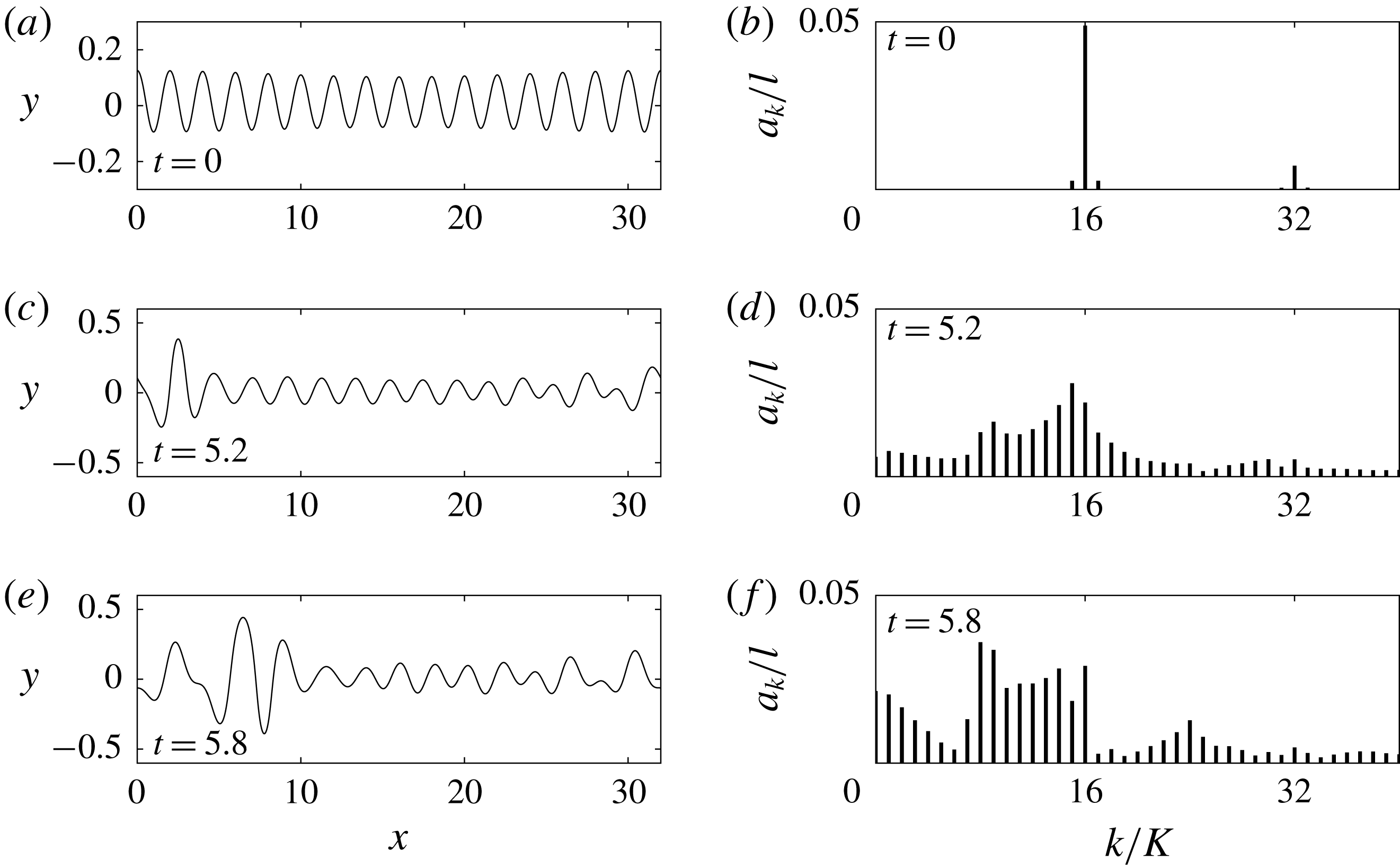
Figure 17. (a,c,e) Time evolution of a Stokes wave with
 $h=10$
,
$h=10$
,
 $\unicode[STIX]{x1D6FA}_{0}=-1$
,
$\unicode[STIX]{x1D6FA}_{0}=-1$
,
 $c=5.2399$
,
$c=5.2399$
,
 $a=0.1$
,
$a=0.1$
,
 $l=2$
,
$l=2$
,
 $\unicode[STIX]{x1D6FD}=0$
,
$\unicode[STIX]{x1D6FD}=0$
,
 $m=16,L=32$
and
$m=16,L=32$
and
 $K=0.1963$
which is initially given a modulational perturbation. The snapshots are taken at
$K=0.1963$
which is initially given a modulational perturbation. The snapshots are taken at
 $t=0$
,
$t=0$
,
 $5.2$
and
$5.2$
and
 $5.8$
. (b,d,f) Fourier spectrum of the wave at
$5.8$
. (b,d,f) Fourier spectrum of the wave at
 $t=0$
,
$t=0$
,
 $5.2$
and
$5.2$
and
 $5.8$
.
$5.8$
.
The next experiment is made in the unstable regime for a long wave
 $h=10$
,
$h=10$
,
 $\unicode[STIX]{x1D6FA}_{0}=-1$
,
$\unicode[STIX]{x1D6FA}_{0}=-1$
,
 $a=0.04$
,
$a=0.04$
,
 $c=0.9219$
,
$c=0.9219$
,
 $l=40\unicode[STIX]{x03C0}$
,
$l=40\unicode[STIX]{x03C0}$
,
 $m=16$
,
$m=16$
,
 $L=640\unicode[STIX]{x03C0}$
,
$L=640\unicode[STIX]{x03C0}$
,
 $\unicode[STIX]{x1D6FC}=0.1$
,
$\unicode[STIX]{x1D6FC}=0.1$
,
 $K=2\unicode[STIX]{x03C0}/L$
,
$K=2\unicode[STIX]{x03C0}/L$
,
 $N=2048$
and
$N=2048$
and
 $\text{d}t=0.1$
. In this gravity dominated case, the instability occurs only after a long time and leads to isolated solitary-like waves appearing as displayed in figure 18. These waves are perturbations of the gravity shallow-water solitary wave, however, due to the flexural terms one expects them to have oscillatory tails.
$\text{d}t=0.1$
. In this gravity dominated case, the instability occurs only after a long time and leads to isolated solitary-like waves appearing as displayed in figure 18. These waves are perturbations of the gravity shallow-water solitary wave, however, due to the flexural terms one expects them to have oscillatory tails.
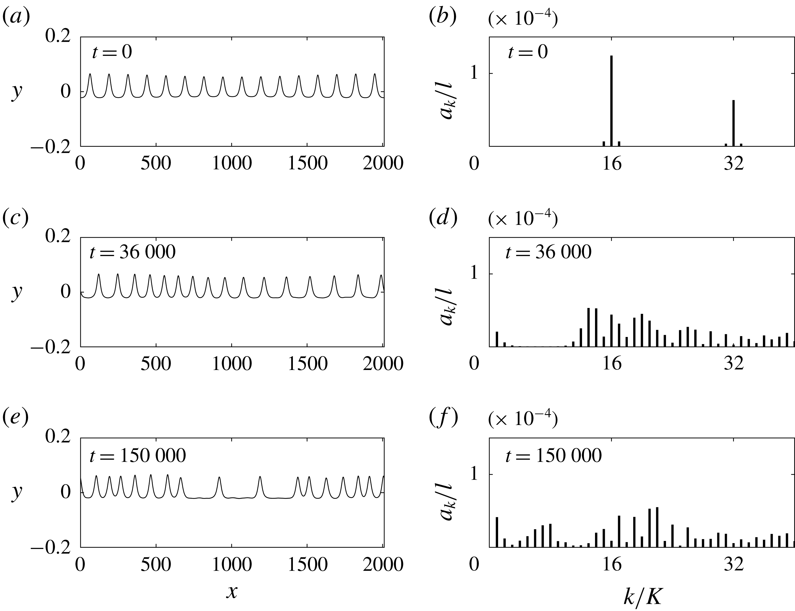
Figure 18. (a,c,e) Time evolution of a Stokes wave with
 $h=10$
,
$h=10$
,
 $\unicode[STIX]{x1D6FA}_{0}=-1$
,
$\unicode[STIX]{x1D6FA}_{0}=-1$
,
 $a=0.04$
,
$a=0.04$
,
 $c=0.9219$
,
$c=0.9219$
,
 $l=40\unicode[STIX]{x03C0}$
,
$l=40\unicode[STIX]{x03C0}$
,
 $\unicode[STIX]{x1D6FD}=0$
,
$\unicode[STIX]{x1D6FD}=0$
,
 $m=16$
,
$m=16$
,
 $L=640\unicode[STIX]{x03C0}$
and
$L=640\unicode[STIX]{x03C0}$
and
 $K=0.0031$
which is initially given a modulational perturbation. The snapshots are taken at
$K=0.0031$
which is initially given a modulational perturbation. The snapshots are taken at
 $t=0$
,
$t=0$
,
 $36\,000$
and
$36\,000$
and
 $150\,000$
. (b,d,f) Fourier spectrum of the wave at
$150\,000$
. (b,d,f) Fourier spectrum of the wave at
 $t=0$
,
$t=0$
,
 $36\,000$
and
$36\,000$
and
 $150\,000$
.
$150\,000$
.
6.2.3 Resonant cases
The numerical framework described here is also useful in examining the modulational stability of the Wilton solutions when the coefficient of the vor-NLS becomes singular due to the second harmonic resonance. We select a fully nonlinear Wilton solution with
 $a=0.018$
,
$a=0.018$
,
 $c=1.5193$
and
$c=1.5193$
and
 $l=11.7322$
for numerical computations of instability. Two experiments are conducted with the following settings
$l=11.7322$
for numerical computations of instability. Two experiments are conducted with the following settings
(i)
$\text{d}t=0.001$
,
$N=1024$
,
$\unicode[STIX]{x1D6FC}=0.1$
,
$L=8l=93.8574$
and
$K=0.0669$
,(ii)
$\text{d}t=0.001$
,
$N=2048$
,
$\unicode[STIX]{x1D6FC}=0.1$
,
$L=16l=187.7148$
and
$K=0.0335$
,


with an initial modulational perturbation (6.4) being imposed. The results are depicted respectively in figures 19(a,c) and 19(b,d). It shows that, for a given solution, the modulational stability of second harmonic resonant travelling wave depends on the value of
 $K$
as expected in standard BF instability. The precise stability condition for this case is expected to have a similar form as (3.44) and will be investigated in future work.
$K$
as expected in standard BF instability. The precise stability condition for this case is expected to have a similar form as (3.44) and will be investigated in future work.
Finally, we examine numerically the modulational stability of a uniform wavetrain when the short-wave/long-wave resonance takes place. By imposing
 $h=10$
,
$h=10$
,
 $\unicode[STIX]{x1D6FA}_{0}=0.1$
and
$\unicode[STIX]{x1D6FA}_{0}=0.1$
and
 $|A|=0.02$
in (3.44), we find the value of the threshold
$|A|=0.02$
in (3.44), we find the value of the threshold
 $K^{\ast }=0.066$
. Two numerical experiments are conducted for a Stokes wave with
$K^{\ast }=0.066$
. Two numerical experiments are conducted for a Stokes wave with
 $l=4.6124$
(
$l=4.6124$
(
 $k=k^{\ddagger }$
),
$k=k^{\ddagger }$
),
 $a=0.02$
and
$a=0.02$
and
 $c=1.5176$
. We carry out two experiments where an initial modulational perturbation (6.4) is imposed with the following parameters
$c=1.5176$
. We carry out two experiments where an initial modulational perturbation (6.4) is imposed with the following parameters
(i)
$\text{d}t=0.0002$
,
$N=2048$
,
$\unicode[STIX]{x1D6FC}=0.1$
,
$L=16l=73.7985$
and
$K=0.0851$
(
${>}K^{\ast }$
),(ii)
$\text{d}t=0.0002$
,
$N=4096$
,
$\unicode[STIX]{x1D6FC}=0.1$
,
$L=32l=147.5971$
and
$K=0.0426$
(
${<}K^{\ast }$
).


In the first example, the modulational stability predicted by the theory due to condition (3.44) is confirmed by the numerical results presented in figure 20(a,c) whilst the instability is discovered in the second one as expected. Therefore analysis from § 3.3 is verified by our numerical computations. Importantly we see the strong generation of a long-wave component in the spectrum. This case is also the subject of future investigations.

Figure 19. (a,b) Time evolution of a Wilton solution with
 $h=10$
,
$h=10$
,
 $\unicode[STIX]{x1D6FA}_{0}=0.1$
,
$\unicode[STIX]{x1D6FA}_{0}=0.1$
,
 $a=0.018$
,
$a=0.018$
,
 $c=1.5193$
,
$c=1.5193$
,
 $l=11.7322$
,
$l=11.7322$
,
 $L=93.8574$
and
$L=93.8574$
and
 $K=0.0669$
which is initially given a modulational perturbation. The snapshots are taken at
$K=0.0669$
which is initially given a modulational perturbation. The snapshots are taken at
 $t=0$
and
$t=0$
and
 $5000$
. (c,d) Fourier spectrum of the wave at
$5000$
. (c,d) Fourier spectrum of the wave at
 $t=0$
and
$t=0$
and
 $5000$
. (b,d) Same as (a,c) for the Wilton solution but with
$5000$
. (b,d) Same as (a,c) for the Wilton solution but with
 $L=187.7148$
and
$L=187.7148$
and
 $K=0.0669$
.
$K=0.0669$
.

Figure 20. (a,b) Time evolution of a uniform wavetrain with
 $h=10$
,
$h=10$
,
 $\unicode[STIX]{x1D6FA}_{0}=0.1$
,
$\unicode[STIX]{x1D6FA}_{0}=0.1$
,
 $a=0.02$
,
$a=0.02$
,
 $c=1.8432$
,
$c=1.8432$
,
 $l=4.6124$
,
$l=4.6124$
,
 $L=73.7985$
and
$L=73.7985$
and
 $K=0.0851$
which is initially given a modulational perturbation. The snapshots are taken at
$K=0.0851$
which is initially given a modulational perturbation. The snapshots are taken at
 $t=0$
and
$t=0$
and
 $2000$
. (c,d) Fourier spectrum of the wave at
$2000$
. (c,d) Fourier spectrum of the wave at
 $t=0$
and
$t=0$
and
 $2000$
. (b,d) Same as (a,c) for the wavetrain with
$2000$
. (b,d) Same as (a,c) for the wavetrain with
 $L=147.5971$
and
$L=147.5971$
and
 $K=0.0426$
.
$K=0.0426$
.
7 Discussion
In this work, we have considered the problem of hydroelastic waves on water of finite depth interacting with a linear shear current within the framework of the nonlinear Schödinger equation and its comparison to numerical solutions of the full Euler equations. The main significance of the vor-NLS in this paper is twofold: to predict the existence of wavepacket solitary waves bifurcating from the minimum of the phase speed and to identify the region of the Benjamin–Feir instability. Direct numerical simulations in the full Euler equations based on the conformal mapping technique have been performed to verify the weakly nonlinear theory and further explore the regime beyond validity of vor-NLS. It is found that the vorticity plays an important role in determining the type of the vor-NLS. However, even when small-amplitude solitary waves are not predicted by the weakly nonlinear theory (namely, the vor-NLS is of defocussing type at the phase speed minimum), we can numerically find large-amplitude solitary waves in the fully nonlinear equations. Similarly, it is shown that large-amplitude wavetrains are unstable subject to modulational perturbations even though their small-amplitude counterparts are in the Benjamin–Feir stable regime. It is also worth mentioning that, in contrast to the pure gravity case, the Benjamin–Feir instability is more complicated in hydroelastic waves. Due to the competing effects of gravity and elastic bending, the wavenumbers of carrier waves can be divided into three categories: a long-wavelength regime where gravity dominates, short-wavelength regime where the elastic effect plays the leading role and the third regime is in vicinity of the phase speed minimum where the two effects are comparable. These different regimes have very different long-time dynamics for modulated wavetrains subject to subharmonic perturbations. In addition, the modulational instabilities of second harmonic resonant and short-wave/long-wave resonant solutions were also investigated by fully nonlinear computations.
In wave–current interactions, the vertical velocity profile of the current is usually nonlinear in practice (for example, when the shear results from bottom friction or wind stress in water-wave problems). However, more general vorticity distributions can be approximated by multi-layer models with linear shear current in each layer. For instance, Milinazzo & Saffman (Reference Milinazzo and Saffman1990) computed the permanent profiles of gravity and gravity–capillary waves in deep water in the presence of a thin layer of constant vorticity mimicking the effect due to wind drift. It is of interest to generalise the asymptotic and numerical results of the present paper to the case of piecewise linear shear currents in future study. Finally we remark that internal waves can induce shear currents, which may also interact with surface ice sheets or man-made very large floating structures. Wang et al. (Reference Wang, Părău, Milewski and Vanden-Broeck2014) recently numerically computed steady internal gravity waves under a flexible elastic sheet, modelling ice cover. It is of particular interest to further study the generation mechanism and the evolution of hydroelastic waves when large-amplitude internal solitary waves propagate under the surface.
Acknowledgements
Z.W. was supported by the National Natural Science Foundation of China (no. 11772341), the Key Research Program of Frontier Sciences, CAS (no. QYZDBSSW-SYS015) and the Strategic Priority Research Program of the Chinese Academy of Sciences (no. XDB22040203). P.A.M. was supported by EPSRC under grant no. EP/N018176/1.
Appendix A
In the non-resonant case, we seek the solution in the form (3.5)–(3.6). In the subsequent analysis, we sketch the derivation of the nonlinear Schrödinger equation. One first solves the Laplace equation at each order
 $n$
and for each harmonic mode
$n$
and for each harmonic mode
 $j$
$j$
 $$\begin{eqnarray}\displaystyle (\unicode[STIX]{x1D719}_{nj})_{yy}-(jk)^{2}\unicode[STIX]{x1D719}_{nj}=P_{nj},\quad (\unicode[STIX]{x1D719}_{nj})_{y}=0\quad \text{at }y=-h, & & \displaystyle\end{eqnarray}$$
where
 $P_{nj}$
is made up of known lower-order terms. The solution to (A 1) has the form
$P_{nj}$
is made up of known lower-order terms. The solution to (A 1) has the form
 $$\begin{eqnarray}\displaystyle \unicode[STIX]{x1D719}_{nj}=\unicode[STIX]{x1D711}_{nj}(X-c_{g}T,\unicode[STIX]{x1D70F})\cosh (jk(y+h))+\unicode[STIX]{x1D719}_{nj}^{p}, & & \displaystyle\end{eqnarray}$$
where
 $\unicode[STIX]{x1D719}_{nj}^{p}$
is a particular solution arising from
$\unicode[STIX]{x1D719}_{nj}^{p}$
is a particular solution arising from
 $P_{nj}$
. Substituting this solution in the surface boundary conditions (3.3)–(3.4) yields
$P_{nj}$
. Substituting this solution in the surface boundary conditions (3.3)–(3.4) yields
 $$\begin{eqnarray}\displaystyle & \displaystyle -j\text{i}\unicode[STIX]{x1D714}A_{nj}-jk\sinh (jkh)\unicode[STIX]{x1D711}_{nj}=Q_{nj}, & \displaystyle\end{eqnarray}$$
 $$\begin{eqnarray}\displaystyle & \displaystyle j\text{i}kgA_{nj}+\frac{D}{\unicode[STIX]{x1D70C}}(j\text{i}k)^{5}A_{nj}+j^{2}\unicode[STIX]{x1D714}k\cosh (jkh)\unicode[STIX]{x1D711}_{nj}-jk\unicode[STIX]{x1D6FA}_{0}\sinh (jkh)\unicode[STIX]{x1D711}_{nj}=R_{nj}, & \displaystyle\end{eqnarray}$$
where
 $Q_{nj}$
and
$Q_{nj}$
and
 $R_{nj}$
are also lower-order terms. At the leading order, the system is homogeneous, namely
$R_{nj}$
are also lower-order terms. At the leading order, the system is homogeneous, namely
 $P_{11}=Q_{11}=R_{11}=0$
, the existence of non-trivial solution results in the dispersion relation
$P_{11}=Q_{11}=R_{11}=0$
, the existence of non-trivial solution results in the dispersion relation
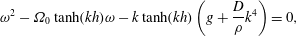 $$\begin{eqnarray}\displaystyle \unicode[STIX]{x1D714}^{2}-\unicode[STIX]{x1D6FA}_{0}\tanh (kh)\unicode[STIX]{x1D714}-k\tanh (kh)\left(g+\frac{D}{\unicode[STIX]{x1D70C}}k^{4}\right)=0, & & \displaystyle\end{eqnarray}$$
and the relation between
 $A_{11}$
and
$A_{11}$
and
 $\unicode[STIX]{x1D711}_{11}$
 $$\begin{eqnarray}\displaystyle \unicode[STIX]{x1D711}_{11}=-\frac{\text{i}\unicode[STIX]{x1D714}}{k\sinh (kh)}\,A_{11}. & & \displaystyle\end{eqnarray}$$
At the next order, we retrieve the group speed
 $c_{g}$
which is defined by
$c_{g}$
which is defined by
 $$\begin{eqnarray}\displaystyle c_{g}={\displaystyle \frac{\unicode[STIX]{x1D6FA}_{0}\unicode[STIX]{x1D714}h\operatorname{sech}^{2}(kh)+\left(g+{\displaystyle \frac{D}{\unicode[STIX]{x1D70C}}}k^{4}\right)kh\operatorname{sech}^{2}(kh)+\left(g+{\displaystyle \frac{5D}{\unicode[STIX]{x1D70C}}}k^{4}\right)\tanh (kh)}{2\unicode[STIX]{x1D714}-\unicode[STIX]{x1D6FA}_{0}\tanh (kh)}}. & & \displaystyle\end{eqnarray}$$
It is not difficult to verify that
 $c_{g}\equiv \unicode[STIX]{x1D714}_{k}$
by directly differentiating (A 5) with respect to
$c_{g}\equiv \unicode[STIX]{x1D714}_{k}$
by directly differentiating (A 5) with respect to
 $k$
. In addition, we obtain the expressions of
$k$
. In addition, we obtain the expressions of
 $A_{22}$
and
$A_{22}$
and
 $\unicode[STIX]{x1D711}_{22}$
in terms of
$\unicode[STIX]{x1D711}_{22}$
in terms of
 $A_{11}^{2}$
as
$A_{11}^{2}$
as
 $$\begin{eqnarray}\displaystyle A_{22}=\frac{D_{1}}{D_{0}}\,A_{11}^{2},\quad \unicode[STIX]{x1D711}_{22}=\frac{D_{2}}{D_{0}}\,A_{11}^{2}, & & \displaystyle\end{eqnarray}$$
where
 $$\begin{eqnarray}\displaystyle & \displaystyle D_{0}=8\text{i}k\cosh ^{2}(kh)\tanh (kh)\left[\unicode[STIX]{x1D714}^{2}\tanh (kh)-\frac{15D}{\unicode[STIX]{x1D70C}}k^{5}\right], & \displaystyle\end{eqnarray}$$
 $$\begin{eqnarray}\displaystyle & \displaystyle D_{1}=4\text{i}k^{2}\cosh ^{2}(kh)\left\{[3-\tanh ^{2}(kh)]\left[gk+\frac{D}{\unicode[STIX]{x1D70C}}k^{5}\right]+\unicode[STIX]{x1D6FA}_{0}^{2}\tanh (kh)\right\}, & \displaystyle\end{eqnarray}$$
 $$\begin{eqnarray}\displaystyle & \displaystyle D_{2}=2k\left[3\unicode[STIX]{x1D714}\coth (kh)\left(gk+\frac{11D}{\unicode[STIX]{x1D70C}}k^{5}\right)-3\unicode[STIX]{x1D714}^{3}+\unicode[STIX]{x1D6FA}_{0}^{2}\unicode[STIX]{x1D714}-\frac{15D}{\unicode[STIX]{x1D70C}}\unicode[STIX]{x1D6FA}_{0}k^{5}\right]. & \displaystyle\end{eqnarray}$$
At the third order,
 $Q_{30}=R_{30}=0$
gives the relation (3.10). Finally, a considerable amount of algebra results in the solvability condition for the mode
$Q_{30}=R_{30}=0$
gives the relation (3.10). Finally, a considerable amount of algebra results in the solvability condition for the mode
 $\text{e}^{\text{i}\unicode[STIX]{x1D6E9}}$
and we obtain the nonlinear Schrödinger equation (3.15). The explicit form of the dispersive coefficient
$\text{e}^{\text{i}\unicode[STIX]{x1D6E9}}$
and we obtain the nonlinear Schrödinger equation (3.15). The explicit form of the dispersive coefficient
 $\unicode[STIX]{x1D706}$
is
$\unicode[STIX]{x1D706}$
is
 $$\begin{eqnarray}\displaystyle \unicode[STIX]{x1D706} & = & \displaystyle {\displaystyle \frac{1}{2\unicode[STIX]{x1D714}-\unicode[STIX]{x1D6FA}_{0}\tanh (kh)}}\left[\left(g+{\displaystyle \frac{5D}{\unicode[STIX]{x1D70C}}}k^{4}+\unicode[STIX]{x1D6FA}_{0}c_{g}\right)h\operatorname{sech}^{2}(kh)\right.\nonumber\\ \displaystyle & & \displaystyle \left.-\,\left(gk+{\displaystyle \frac{D}{\unicode[STIX]{x1D70C}}}k^{5}+\unicode[STIX]{x1D6FA}_{0}\unicode[STIX]{x1D714}\right)h^{2}\operatorname{sech}^{2}(kh)\tanh (kh)+{\displaystyle \frac{10D}{\unicode[STIX]{x1D70C}}}k^{3}\tanh (kh)-c_{g}^{2}\right].\qquad\end{eqnarray}$$


