2.1. Scaling

In the reduction of the governing equations performed by Ball & Balmforth (Reference Ball and Balmforth2021), the dimensions are removed from the problem by scaling vertical and radial distances by the characteristic scales $\mathcal H$ and $\mathcal L$ , respectively. The horizontal velocity components $u$ and $v$ are scaled by ${\mathcal V}=Q/({\mathcal H}{\mathcal L})$ , and the vertical velocity $w$ by ${\mathcal H}{\mathcal V}/{\mathcal L}$ , where $Q$ is the volume flux. Time is scaled by ${\mathcal T}={\mathcal L}/{\mathcal V}$ . The stresses and pressure are scaled by the hydrostatic scale $\rho g' {\mathcal H}$ .

The Herschel–Bulkley law has three parameters: the yield stress ${\tau _{_{\textrm { Y}}}}$ , the power-law index $n$ and the consistency $K$ . This constitutive law relates the (dimensional) second invariants of the stress, $\tau$ , and deformation-rate tensor, $\dot \gamma$ , through $\tau ={{\tau _{_{\textrm { Y}}}}}+K{\dot \gamma }^n$ (Balmforth et al. Reference Balmforth, Frigaard and Ovarlez2014). The consistency $K$ and characteristic strain rate, ${\mathcal V}/{\mathcal L}$ , can be combined into a stress scale $K({\mathcal V}/{\mathcal L})^n$ which, when balanced with $\rho g' {\mathcal H}$ provides the vertical length scale

(2.1) \begin{equation} {\mathcal H} = \left (\frac {\textit{KQ}^n}{\rho g' {\mathcal L}^{2n}}\right )^{\frac {1}{n+1}} . \end{equation}

Hence

(2.2) \begin{align} {\mathcal T} = \frac {{\mathcal H}{\mathcal L}^2}{Q} = \left (\frac {K\!{\mathcal L}^2}{\rho g' Q}\right )^{\frac {1}{n+1}}. \end{align}

Two parameters remain from the scaling of the Herschel–Bulkley law: the power-law index $n$ and a Bingham number related to the dimensional yield stress ${\tau _{_{\textrm { Y}}}}$

(2.3) \begin{equation} \textit{Bi} = \frac {{{\tau _{_{\textrm { Y}}}}} {\mathcal H}^n{\mathcal L}^{2n}}{\textit{KQ}^n} = {{\tau _{_{\textrm { Y}}}}} \left (\frac {{\mathcal L}^{2}}{\rho g' K^{\frac {1}{n}} Q}\right )^{\frac {n}{n+1}} . \end{equation}

The parameters $n$ and $\textit{Bi}$ feature in our model solutions; we exploit the time scale $\mathcal T$ in our interrogation of experimental results.

The scales above can be used to gauge the importance of physical effects that are not incorporated into the model. For example, to estimate the importance of viscous drag from the bath, we note that, although the bath is deep relative to the film thickness, it remains shallower than $\mathcal L$ . The main drag therefore stems from vertical shear stresses, of order $\mu _b {\mathcal V}/{\mathcal H}_b$ , if $\mu _b$ and ${\mathcal H}_b$ are the viscosity and depth of the bath. The vertical shear stress in the film, on the other hand, is $O(\rho g' {\mathcal H}^2/{\mathcal L})$ . The importance of drag can therefore be measured by the ratio

(2.4) \begin{equation} \frac {\mu _b {\mathcal V}{\mathcal L} }{\rho g' {\mathcal H}^2 {\mathcal H}_b} \equiv \frac {\mu _b}{{\mathcal H}_b}\left [\frac {(\rho g')^{2-n}Q^{1-2n}{\mathcal L}^{6n}}{K^3}\right ]^{\frac {1}{n+1}}. \end{equation}

Estimates based on our experiments in § 3 (table 1) indicate that this ratio is $O(10^{-4})-O(10^{-2})$ . Hence, drag from the bath is not significant. That said, once the film spreads sufficiently far from the launch stage, the radius of the pedestal is not necessarily the best choice for the horizontal length scale $\mathcal L$ . Nevertheless, we observed no significant differences in the dynamics when a subset of the experiments were repeated with a bath of almost twice the depth. The omission of surface tension is a little more tricky to justify, an issue we return to later.

2.2. Model equations

In the polar coordinates $(r,\vartheta )$ , the dimensionless mathematical model combines the depth-integrated conservation of mass and momentum equations for the fluid depth $h(r,\vartheta ,t)$ and horizontal velocity $(u,v)$ , with the leading-order Herschel–Bulkley constitutive law relating the horizontal stresses $\{\tau _{\textrm { rr}},\tau _{\textrm {r}\theta },\tau _{\theta \theta }\}$ and strain rates $\{{\dot \gamma }_{\textrm { rr}},{\dot \gamma }_{\theta \theta },{\dot \gamma }_{\textrm {r}\theta }\}$ . The model equations are

(2.5) \begin{align} \frac {\partial h}{\partial t} +\frac {1}{r}\frac {\partial }{\partial r}(r hu) +\frac {1}{r}\frac {\partial }{\partial \vartheta }\left (vh\right ) = 0 , \end{align}

(2.6) \begin{align} \frac {\partial }{\partial r} \left [ {\mbox {$1\over 2$}} h^2 - h(2\tau _{\textrm { rr}}+\tau _{\theta \theta })\right ] - \frac {1}{r}\frac {\partial }{\partial \vartheta }\left (h\tau _{\textrm {r}\theta }\right ) + \frac {h}{r}(\tau _{\theta \theta }-\tau _{\textrm { rr}}) = 0 , \end{align}

(2.7) \begin{align} \frac {1}{r}\frac {\partial }{\partial \vartheta } \left [ {\mbox {$1\over 2$}} h^2 - h(2\tau _{\theta \theta }+\tau _{\textrm { rr}})\right ] - \frac {\partial }{\partial r} \left (h\tau _{\textrm {r}\theta }\right ) -\frac {2}{r}h\tau _{\textrm {r}\theta } = 0. \end{align}

(2.8) \begin{equation} \left \{ \begin{aligned} \dot \gamma &= 0,& \tau \lt \textit{Bi},\\ [\tau _{\textrm { rr}},\tau _{\theta \theta },\tau _{\textrm {r}\theta }] &= \left (\frac {\textit{Bi}}{{\dot \gamma }}+{\dot \gamma }^{n-1}\right ) \left [{\dot \gamma }_{\textrm { rr}},{\dot \gamma }_{\theta \theta },{\dot \gamma }_{\textrm {r}\theta }\right ] , & \tau \geq \textit{Bi}, \end{aligned}\right . \end{equation}

with

(2.9) \begin{equation} \left [{\dot \gamma }_{\textrm { rr}},{\dot \gamma }_{\theta \theta },{\dot \gamma }_{\textrm {r}\theta }\right ] = \left [2\frac {\partial u}{\partial r}, \frac {2}{r}\left (u+\frac {\partial v}{\partial \vartheta }\right ), \frac {1}{r}\left (\frac {\partial u}{\partial \vartheta }-v\right )+\frac {\partial v}{\partial r}\right ] , \end{equation}

where ${\dot \gamma }=\sqrt {{\dot \gamma }_{\textrm { rr}}^2+{\dot \gamma }_{\textrm {r}\theta }^2+{\dot \gamma }_{\theta \theta }^2 +{\dot \gamma }_{\textrm { rr}}{\dot \gamma }_{\theta \theta }}$ and $\tau =\sqrt {\tau _{\textrm { rr}}^2+\tau _{\textrm {r}\theta }^2+\tau _{\theta \theta }^2+\tau _{\textrm { rr}}\tau _{\theta \theta }}$ .

At the outer edge, $r=R(\vartheta ,t)$ , we impose the kinematic condition, and demand that the net normal and tangential stresses vanish

(2.10) \begin{equation} \frac {\partial R}{\partial t}+\frac {v}{R}\frac {\partial R}{\partial \vartheta }=u, \end{equation}

(2.11) \begin{equation} \frac {1}{2}h^2-h\left [\tau _{\textrm { rr}}+\tau _{\theta \theta }+\frac {R}{\sqrt {R^2+R_{\vartheta }^2}}\left (\tau _{\textrm { rr}} -2\frac {R_{\vartheta }}{R}\tau _{\textrm {r}\theta }+\frac {R_{\vartheta }^2}{R^2}\tau _{\theta \theta }\right )\right ]=0, \end{equation}

(2.12) \begin{equation} \tau _{\textrm {r}\theta }-\frac {R_{\vartheta }}{R}(\tau _{\theta \theta }-\tau _{\textrm { rr}})-\frac {R_{\vartheta }^2}{R^2}\tau _{\textrm {r}\theta }=0 . \end{equation}

Here and below we use the subscripts $(r,\vartheta )$ to denote partial derivatives, which can be distinguished by typeface from our notation $(\rm { r,\theta })$ for the tensor components.

We position the inner edge of the film slightly beyond the radius of the pedestal, at $r=1+\varepsilon$ with $\varepsilon \ll 1$ . Here, we impose the incoming flux and angular velocity

(2.13) \begin{equation} 2\pi hu=1, \quad v=0 . \end{equation}

The abrupt increase in film thickness, implied by the match to the incoming gravity current over the pedestal, can be imposed by taking $h(1+\varepsilon ,t)$ to diverge suitably for $\varepsilon \to 0$ , as we explain below.

2.3. Axisymmetric spreading solutions

From (2.6)–(2.8), axisymmetric spreading states, with

\begin{align*} h = H(r,t), \ u = U(r,t), \ v = 0, \ R = \overline {R}(t), \ [\tau _{\textrm { rr}},\tau _{\textrm {r}\theta },\tau _{\theta \theta }] = [{T_{\textrm { rr}}}(r,t),0,{T_{\theta \theta }}(r,t)] , \end{align*}

satisfy the equations

(2.14) \begin{align} H_t+\frac {1}{r}(r HU)_r &= 0 , \end{align}

(2.15) \begin{align} \left [\frac {1}{2}H^2 - H(2{T_{\textrm { rr}}}+{T_{\theta \theta }})\right ]_r + \frac {H}{r}({T_{\theta \theta }}-{T_{\textrm { rr}}}) &= 0, \end{align}

(2.16) \begin{equation} [{T_{\textrm { rr}}},{T_{\theta \theta }}] = \left (\frac {\textit{Bi}}{{\dot \Gamma }}+{\dot \Gamma }^{n-1}\right ) \left [2U_r, \frac {2U}{r}\right ] , \qquad {\dot \Gamma } = 2\sqrt { U_r^2 + \frac 1r UU_r + \frac {1}{r^2} U^2 }, \end{equation}

along with the boundary conditions

(2.17) \begin{equation} \left [\frac {1}{2}H^2-H(2{T_{\textrm { rr}}}+{T_{\theta \theta }})\right ]_{r=\overline {R}} = 0, \quad \left .2\pi HU\right |_{r\to 1}=1, \end{equation}

and

(2.18) \begin{equation} \overline {R}_t = U(\overline {R},t), \end{equation}

extending the shorthand subscript notation for partial derivatives to $t$ .

Very close to the pedestal when $r-1=O(\varepsilon )\ll 1$ , the radial derivatives become $O(\varepsilon ^{-1})$ . The main balances in (2.14)–(2.16) are then

(2.19) \begin{equation} (HU)_r\sim 0, \quad \left ({\mbox {$H^2/2$}} - 2H{T_{\textrm { rr}}} \right )_r \sim 0, \quad {T_{\textrm { rr}}} \sim 2^n |U_r|^{n}\mathrm {sgn}( U_r) \gg {T_{\theta \theta }} , \end{equation}

implying that the dynamics is controlled by the radial, power-law viscous stress. Hence,

(2.20) \begin{equation} H \sim \frac {1}{2\pi U} \quad \mathrm {and} \quad {T_{\textrm { rr}}} \sim {\frac {1}{4}H} \sim \frac {1}{8\pi U} , \end{equation}

given that $T_{\textrm { rr}}$ must decline to $O(1)$ values further from the pedestal. Consequently,

(2.21) \begin{equation} U \sim \left [\frac {(1+n)^n}{8\pi (2n)^n}(r-1)^n\right ]^{\frac {1}{n+1}} \quad \mathrm {and} \quad H \sim 4\left [4\pi \frac {(1+n)}{n}(r-1)\right ]^{-\frac {n}{n+1}} . \end{equation}

For early times, the kinematic condition in (2.17) also implies that

(2.22) \begin{equation} \overline {R} \sim 1 + \frac {t^{n+1}}{8\pi (2n)^n(n+1)} . \end{equation}

We translate the preceding results into effective boundary and initial conditions as follows: instead of dealing with diverging conditions for $r\to 1$ , we instead place the inner edge of the computation at $r=1+\varepsilon$ . Here, we fix $H(1+\varepsilon ,t)$ and $U(1+\varepsilon ,t)$ using (2.21). To commence computations, we then begin at a time $t=t_0\gt 0$ for which the outer radius is at $R(t_0)=1+2\varepsilon$ , and $U(r,t_0)$ and $H(r,t_0)$ are again given by (2.21). The initial moment $t_0$ can be determined from (2.22), given a suitable choice for $\varepsilon$ .

To advance solutions in time from this initial state, we first discretize in $t$ . Then, at each time and given the current profile of $H(r,t)$ , we solve the boundary-value problem (2.15)–(2.17) for $U(r,t)$ using Matlab’s in-built solver bvp4c. With the computed velocity field $U(r,t)$ in hand, we next employ (2.14) and (2.18) to advance the thickness $H(r,t)$ and outer edge $R(t)$ to a new time, using a Lagrangian scheme. The time step is chosen sufficiently small that mass is conserved to less than $3\, \%$ over the duration of the computation.

Figure 3. (a,b,c) Axisymmetric solutions for the values of $(n,\textit{Bi},\varepsilon )$ indicated. Shown are film profiles at equivalent outer radii, for baths with density ratios $0.83$ (panel (a)) and $\rho /\rho _b=0.54$ (panels (b,c)). The profiles of $H(r,t)$ are replotted on a loglog scale in (d) and compared with (2.21) (red dashed lines). Panel (e) shows time series of the outer radius $\overline {R}(t)$ for the three solutions, with the (red) dashed lines showing (2.22). In (d) and (e) the modified early time solution (2.23) for $\textit{Bi}=1$ is shown by the (red) dotted lines.

Sample numerical solutions for axisymmetric spreading films are presented in figure 3. Panels (a–d) present series of snapshots of the film profile and $H(r,t)$ for Newtonian, power-law and Bingham fluids; corresponding time series of the outer radius $\overline {R}(t)$ are plotted in (e). The density ratios chosen for these solutions are similar to those for (a) syrup spreading on oil ( $\rho /\rho _b=1.54/1.85=0.83$ ) and (b,c) Carbopol or Xanthan gum on oil ( $\rho /\rho _b=1/1.85=0.54$ ). The solutions mostly demonstrate a match with the expected early-time behaviour for $t\ll 1$ , and are not evolved sufficiently far to observe an entrance to the long-time self-similar states for $t\gg 1$ , catalogued in Ball & Balmforth (Reference Ball and Balmforth2021).

Note that the Bingham computation does not converge particularly closely to the early time solution in (2.21)–(2.22) for the value of $\varepsilon =10^{-6}$ chosen (see panel (d)). It turns out that, for these parameter settings, and for most of the computations with finite $\textit{Bi}$ , it is a relatively poor approximation to neglect the yield stress in (2.16) for $T_{\textrm { rr}}$ . If we instead keep this term, we recover an alternative approximation in which $U$ satisfies

(2.23) \begin{equation} \frac {2(8\pi )^{1/n} n}{n+1} U^{\frac {n+1}{n}} {}_2F_1\left (\frac {n+1}{n},\frac {1}{n};\frac {2n+1}{n};8\pi \textit{Bi} U\right ) =r-1, \end{equation}

where ${}_pF_q(a;b;c;z)$ is the generalized hypergeometric function of order $\{p,\,q\}$ . The radius $\overline {R}(t)$ then follows from inverting (2.23) and using the kinematic condition in (2.17). As shown in figure 3(d,e), this alternative approximation is superior to the asymptotic solution in (2.21)–(2.22).

In the linear stability analysis below, we use values of $\varepsilon =10^{-5}-10^{-4}$ to commence the base state solution. This choice ensures that the inner boundary condition achieves a match to a solution with a diverging incoming depth that is otherwise independent of the precise choice for $\varepsilon$ . Simultaneously, the choice ensures that radial gradients remain well resolved over the duration of the computation. Our inner boundary condition therefore avoids any need to match with a full Stokes-type solution at the edge of the pedestal, or impose a prescribed incoming flow depth $H_0$ , as in Ball & Balmforth (Reference Ball and Balmforth2021), which would introduce arbitrary parameter that we cannot calibrate. Nevertheless, our boundary condition is equivalent to prescribing the incoming fluid depth, but then taking the limit $H_0\gg 1$ , leaving a solution that nearly diverges for $r\to 1$ , but otherwise becomes independent of that parameter. Finally, having chosen $\varepsilon$ , we compute the corresponding initial moment $t_0$ using (2.22) if $\textit{Bi}=0$ . To avoid the relatively weak convergence to the small-time limit when $\textit{Bi}\gt 0$ , however, we instead use the alternative approximation in (2.23).

2.4. Stability analysis

To study non-axisymmetric perturbations to the axisymmetric base states, we set

(2.24) \begin{equation} h = H(r,t)+\hat h(r,t)e^{im\vartheta }, \quad u = U(r,t)+\hat u(r,t)e^{im\vartheta }, \end{equation}

(2.25) \begin{equation} v = \hat v(r,t)e^{im\vartheta }, \quad R = \overline {R}(t) +\hat R(t)e^{im\vartheta }, \end{equation}

where $m$ is the angular wavenumber. The linear stability equations are the same as those in Ball & Balmforth (Reference Ball and Balmforth2021) (their equations (4.3)–(4.11)) and are restated in Appendix A. At the inner boundary $r=1+\varepsilon$ , we further adopt the boundary conditions

(2.26) \begin{equation} \hat {u}=\hat {h}=\hat {v}=0 , \end{equation}

assuming that the incoming flow cannot be perturbed. Finally, we use the initial conditions

(2.27) \begin{equation} \hat {R}=\hat {R}_0, \quad \hat {h}=\hat {u}=\hat {v} =0, \quad \textrm { at}\ t=t_0. \end{equation}

2.4.1. Early times, t ≪ 1

At early times, the film forms a relatively narrow annulus where radial derivatives are amplified. Provided $m=O(1)$ , we may then follow a very similar analysis to that presented earlier, with the angular dependence not featuring to leading order. In view of the inner boundary and initial conditions, the perturbation to the radial velocity $\hat {u}$ remain small, and the dynamics becomes slaved to the motion of the outer edge. Considering the early time behaviour close to the pedestal, the perturbation to the outer radius then satisfies the leading-order kinematic condition (see Appendix (A11))

(2.28) \begin{equation} \hat {R}_t \sim U_{r}(\overline {R}) \hat {R}. \end{equation}

Combining with $\overline {R}_t=U(\overline {R})$ , we find

(2.29) \begin{equation} \hat {R}(t)\propto U(\overline {R}). \end{equation}

For $\textit{Bi}\to 0$ , we find

(2.30) \begin{equation} \hat {R}(t) = \hat {R}(t_0) \left [\frac {\overline {R}(t)-1}{\overline {R}(t_0)-1}\right ]^{\frac {n}{n+1}} = \hat {R}(t_0) \left (\frac {t}{t_0}\right )^n . \end{equation}

Although the perturbation grows with time, it does not in comparison with the axisymmetric base state: here $\hat {R}/(\overline {R}-1) \propto t^{-1}$ .

In this early-time limit, the effect of the fluid rheology is therefore felt only through the background velocity gradient, and $\hat {R}(t)$ increases fastest for Newtonian fluid ( $n=1$ ). The growth of the perturbation corresponds to the geometrical spreading effect discussed by Sayag & Worster (Reference Sayag and Worster2019b ), which here factors in the thinning of the base state at the outer edge, as well as its stretching due to axisymmetric expansion. To see any sign of the Sayag & Worster instability (at order-one azimuthal wavenumbers), we must therefore proceed to later times.

2.4.2. Later times, t = O(1)

A numerical solution to the linear stability equations for Newtonian fluid ( $n=1$ , $\textit{Bi}=0$ ) is shown in figure 4 for the mode with angular wavenumber $m=2$ . The amplitude of the perturbation to the radius first grows linearly with time as predicted by (2.30), before slowing down to approach a scaling $t^{-0.8}$ . This dependence is predicted by the analysis of long-time ( $t\gg 1$ ) self-similar solutions to the problem provided in Ball & Balmforth (Reference Ball and Balmforth2021) (their Appendix A). Despite the different boundary conditions applying for $r\to 1$ , this analysis applies here because, in the long time limit, the perturbations decay relatively quickly on proceeding inwards from the outer edge, eliminating any dependence on the conditions at the inner edge. The strengthening inward decay of the solutions can be observed in figure 4(b,c,d), and the final panel compares $\hat {u}$ and $\hat {v}$ with the corresponding self-similar solutions. Consequently, for $t\gg 1$ , the linear modes are all still expected to decay relative to the expansion of the background axisymmetric state, regardless of the value of $m$ , as explored in more detail by Ball & Balmforth (Reference Ball and Balmforth2021). Note that the solution, as with all those we present here, still lies a good way off the self-similar limit.

Figure 4. (a) Time series of the amplitude of the perturbation to the radius $\hat {R}$ scaled by its initial value, for a Newtonian film ( $n=1$ , $\textit{Bi}=0$ , $\varepsilon =10^{-4}$ ) with angular wavenumber $m=2$ . The dot-dashed line shows the prediction in (2.30) and the dashed line indicates the long-time self-similar scaling (Ball & Balmforth Reference Ball and Balmforth2021). In the inset, the amplitude is scaled by $\overline {R}-1$ , then plotted againt $\overline {R}^2-1$ . The spatial structure of the perturbations ( $\hat {u},\hat {v},\hat {h})/\hat {R}$ is shown in (b,c,d) for the times indicated in (a). In (e) the velocity perturbations are scaled by $|\hat {v}(\overline {R},t)|$ and plotted against $r/\overline {R}(t)$ ; the dashed lines show the similarity solution from Ball & Balmforth (Reference Ball and Balmforth2021).

Figure 5. (a) Time series of $|\hat {R}|/[\overline {R}-1]$ against $\overline {R}^2-1$ for a viscoplastic film ( $n=0.4$ , $\textit{Bi}=1$ , $\varepsilon ={10^{-4}}/{4}$ ) with angular wavenumbers $m=1,2,\ldots ,6$ (from green to blue, with $m=1$ shown dashed). The dotted black line shows the prediction in (2.30). Snapshots of scaled height and velocity perturbations $(\hat {h},\hat {u},\hat {v})/\hat {R}$ are shown in (b–d) for $m=2$ , at the times indicated by stars in (a).

Low-angular-wavenumber solutions for a viscoplastic film ( $n=0.4$ , $\textit{Bi}=1$ ) are shown in figure 5. Unlike the Newtonian case, the mode amplitudes now begin to grow relative to the base state at large times, as found in Ball & Balmforth (Reference Ball and Balmforth2021). For the modes shown, with $m=1-6$ , growth begins when the base state has reached dimensional radii of almost $3{\mathcal L}$ . Eventually, provided the solutions all reach the self-similar plastic plate explored in Ball & Balmforth (Reference Ball and Balmforth2021), the growth of the modes is expected to become exponential, with a rate that increases with $m$ . For the experimentally relevant times plotted in figure 5 ( $\overline {R}^2-1\lt 10$ ), however, the modes have yet to reach this limit and are growing comparably to one another, except for the $m=1$ mode which upturns more slowly. The spatial structure of the modes for $m=2$ is relatively simple (figure 5(b,c,d)); more spatial oscillations appear at smaller radii with higher $m$ (cf. Sayag & Worster (Reference Sayag and Worster2019b ); Ball & Balmforth (Reference Ball and Balmforth2021)).

The effect of increasing $\textit{Bi}$ whilst holding $m$ and $n$ fixed is illustrated in figure 6. For the small-time approximation in (2.23), the base state solution remains dependent on $\textit{Bi}$ . As a result, when the initial radius, $\overline {R}(t_0)=1+2\varepsilon$ , is translated to an initial time $t=t_0$ using (2.23), it implies that linear stability computations with different $\textit{Bi}$ are initiated at different times for a fixed $\varepsilon$ . To flatten the landscape for an unbiased comparison, some scaling of the linear stability computations is therefore needed. In view of (2.29), we adopt the scaling factor

(2.31) \begin{equation} \lambda (\textit{Bi})=\frac {U(\overline {R}(t_0(\textit{Bi})))}{[U(\overline {R}(t_0(\textit{Bi})))]_{\textit{Bi}=1}}, \end{equation}

which suppresses the differences in the perturbation $\hat {R}$ introduced by changing the time of initialization, and assures a common limit for $t\to 0$ . In figure 6, we show radius perturbations scaled by $\lambda (\textit{Bi})$ . At early times, the radius perturbation decays, with a rate that increases with yield stress. But for the largest times shown in the figure, the base state expands sooner towards the final, yield-stress-dominated, self-similar state for higher $\textit{Bi}$ (cf. figure 11 of Ball & Balmforth (Reference Ball and Balmforth2021)). As a consequence, the relatively strong instability in the self-similar state appears earlier. The two effects counter one another somewhat, leading to solutions that depend relatively mildly on Bingham number in figure 6. Indeed, for experimentally relevant times (corresponding to mean areas $\overline {R}^2-1\lt 10$ or so), figure 6 suggests that instability is weak and largely independent of $\textit{Bi}$ .

Figure 6. Time series of $\lambda (\textit{Bi})|\hat {R}|/[\overline {R}-1]$ against $\overline {R}^2-1$ for a viscoplastic film with varying $\textit{Bi} = 1, 2,3,4,5,6$ (from blue to red), with $m=2$ , $n=0.4$ and $\varepsilon ={10^{-4}}/{4}$ . The dashed black lines shows the prediction in (2.29) for $\textit{Bi}=2$ and 6; the dotted black line shows the prediction in (2.30) for $\textit{Bi}=0$ .

Results for a power-law fluid film ( $n=0.12$ and $\textit{Bi}=0$ ) are shown in figure 7. As in the Newtonian case, the modes initially grow as expected by (2.30), decaying relative to the base state flow. The spatial structure of the modes is similar to that seen for the viscoplastic film in figure 5. At early times, modes with higher-wavenumber decay slightly faster, a trend that eventually reverses. The most conspicuous feature seen in figure 7(a) is the onset of oscillatory growth for $m\gt 1$ at the final times, a feature noted previously in Ball & Balmforth (Reference Ball and Balmforth2021). This leads to a node in the mode amplitude $|\hat {R}|$ , visible as the sharp negative spike in the logarithmic plot in figure 7(a). The non-zero frequency suggests that patterns form pulsating standing waves or rotate in angle in the manner of a travelling wave, depending on initial conditions. Oscillatory growth also arises for finite $\textit{Bi}$ ; the solutions for larger values of $m$ in figure 5(a) are on the brink of such behaviour, which accounts for the downturn in the amplitude for the mode with highest $m$ at the right end of the plot.

Figure 7. (a) Time series of $|\hat {R}|/[\overline {R}-1]$ against $\overline {R}^2-1$ for a power-law film ( $n=0.12$ , $\textit{Bi}=0$ , $\varepsilon = {10^{-4}}/{4}$ ) with angular wavenumbers $m=1,2,\ldots ,6$ (from green to blue, with $m=1$ shown dashed). The dotted black line shows the prediction in (2.30). Snapshots of scaled height and velocity perturbations $(\hat {h}, \hat {u},\hat {v})/\hat {R}$ are shown in (b–d) for $m=2$ , at the times indicated in (a).

3.1. Set-up

To complement theory, we conducted a series of experiments in which a complex fluid was floated out on top of a bath of denser viscous fluid, as illustrated in figure 2. For the complex fluid we used aqueous suspensions of either Carbopol, with concentration 0.2 % (Ultrez 21, neutralized with sodium hydroxide), or Xanthan gum, with concentration 0.6 %. Fits to the flow curves of these fluids, as measured in a Kinexus Malvern rheometer (employing roughened parallel plates and a controlled decreasing shear-rate ramp) are shown in figure 8. Parameter values and relevant dimensionless groups are presented in table 1. Note that the fastest radial speeds in the experiments are of order a few millimetres per second, over radial scales of a few centimetres, implying strain rates of $0.1\,$ $\rm s^{-1}$ or less. Viscoelastic relaxation times for Carbopol and Xanthan gum are commonly quoted to be a second or less. Therefore, Weissenberg numbers are expected to be relatively small, suggesting that fluid viscoelasticity is not relevant.

Figure 8. Flow curves for the two complex fluids used in the experiments. In these decreasing shear-rate ramps, there are ten samples per decade of shear rate, and a 60 s wait time at each $\dot \gamma$ to reach steady state. The points show the rheometer measurements, the lines indicate the fits in table 1.

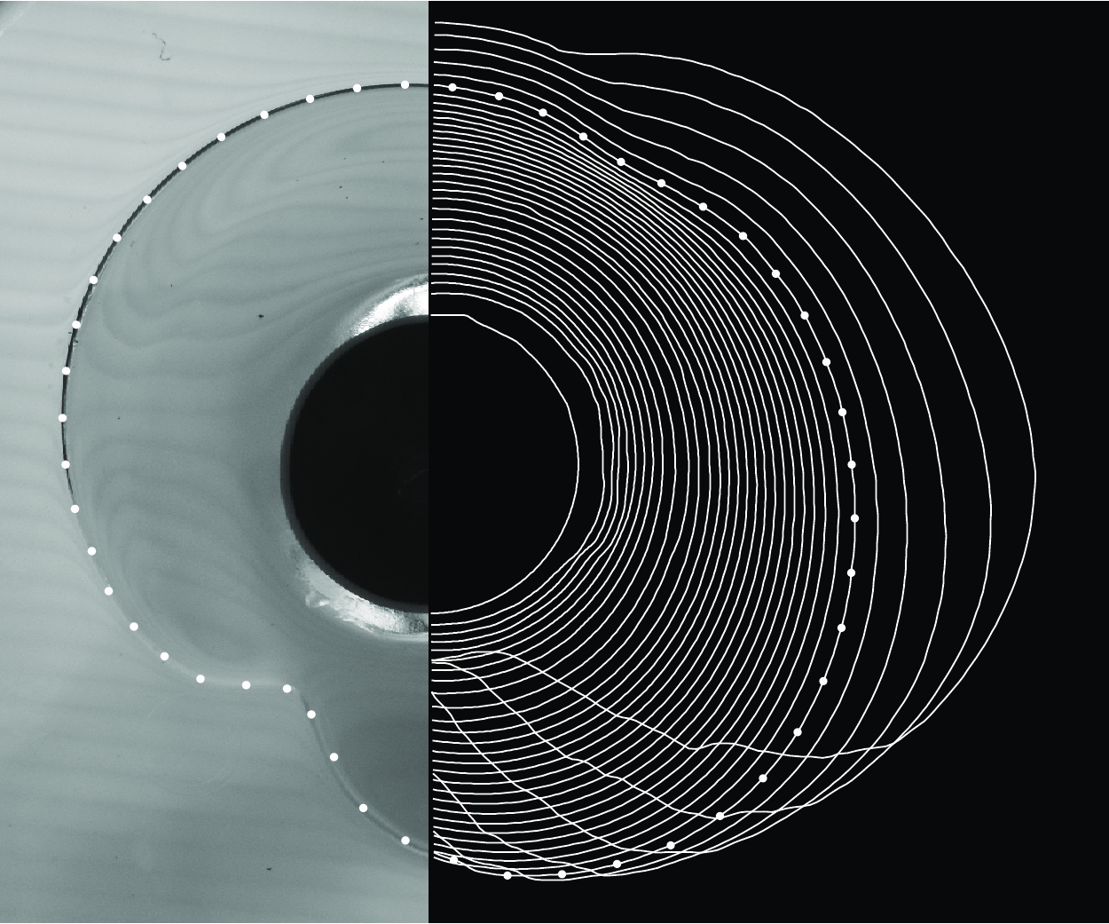
Figure 9. (a)–(c) Photographs from below and (d) extracted outlines of the fluid edge for an experiment with Carbopol pumped above an oil bath of depth $10.5\,$ mm with flux $20\,$ ml/min. The reconstruction of the edge outline from the photograph is also indicated in (c) as a green dashed line, as is the outer edge of the pedestal (green solid line). Three other tests for the same experimental conditions are shown in (e). In (d), the outlines are 5 s apart; in (e), the interval is 10 s. These outlines are coloured by time, from green to blue. The pedestal (shown in black in (a–c) and shaded grey in (d,e)) has a radius of $1.7\,$ cm.

The bath was filled up to the top with a perfluoropolyether oil (Galden HT 270, Lesker Cor.). A pedestal with a height equal to the depth of the bath ${\mathcal H}_b$ was placed in the centre of the bath to act as a launch stage for the complex fluid, which was emplaced from a tube connected to a syringe pump delivering constant flux $Q$ . Once the film of complex fluid spread out over the bath, any displaced oil flowed over the brim to help maintain the level of the bath. Images taken of the film from below were processed to extract the outer edge (see figure 9). A second camera positioned at the level of the bath was used to record side images of the floating film and to look for any changes in the depth of the surrounding oil. No such changes in depth were observed, and capillary effects along the outer brim of the bath did not appear to be significant.

3.2. First observations

The observed phenomenology of experiments with Carbopol is illustrated in figure 9, which presents three successive images (taken from above) of the expanding floating film in one of the experiments. Also displayed are reconstructed outlines of the outer edge for this particular test, and for three other repetitions of it. After pumping commenced, the fluid deposited on the pedestal spreads out, eventually reaching the edge of the pedestal and coming into contact with the oil. The film then floated out above the bath, initially in a roughly axisymmetrical manner, modulo any imperfections associated with a non-axisymmetric contact with the oil at the edge of the pedestal (figure 9 a,b). At later times, however, the film significantly lost axisymmetry as one or two ‘clefts’ appeared at the outer edge (figure 9 c). These defects grew, diverting fluid sideways, with their roots retreating backwards and often rotating around the pedestal (figure 9 d). As illustrated in figure 10, this phenomenology spanned the entire range of experiments with Carbopol performed with varying flux.

In repetitions of the tests with the same experimental parameter settings, the clefts appeared at differing angular positions (see figure 9 e). Similarly, in figure 10 the clefts have no preferred angular orientation. Thus, there appear to be no angular bias in the tests due to an imperfect experimental set-up. That said, however, the angular position at which a cleft formed did, on occasion, appear to be correlated with the location where the complex fluid film first flowed out from the pedestal, as can be seen by careful inspection of the early contours in figures 9 and 11.

Figure 10. Outlines of the fluid edge for experiments with Carbopol (from above, coloured by time, from green to blue) for tests with increasing flux (proceeding from left to right with $Q=1.25$ , $2.5$ , 5, 10, 40, 60, 80, 120 ml/min). The intervals between these outlines varies between experiment.

The dynamics was similar in tests with Xanthan gum, as illustrated in figure 11. For this material, however, the clefts responsible for prompting non-axisymmetric patterns were much more rounded and developed after a longer time. The degree of asymmetry in the final patterns was also less pronounced.

Figure 11. Outlines of the fluid edge for experiments with Xanthan gum for the fluxes indicated. The outlines are 10 s apart and coloured by time, from green to blue.

Images taken from the side of the experiment for films of both Carbopol and Xanthan gum are illustrated in figure 12. The thinning of the film as it descends off the pedestal is clear, as is the much flatter floating film that then forms (cf. figure 3). At the outer edge of the film, the fluids are visibly rounded off, and probably thickened, by surface tension. Such features, coupled with the perspective of the camera, make thicknesses hard to estimate. Nevertheless, both images suggest that the film is several millimetres thick, given that submergences of a factor of two or so are expected from the density differences. Such depths are larger than our estimates for the characteristic height scale $\mathcal H$ in the theoretical model, as quoted in table 1. That said, the dimensionless film depths achieved in model solutions suggest that actual depths can be larger than $\mathcal H$ by factors of order unity (see figure 3). More awkward is the rounding of the film profile at the outer edge, which suggests a prominent effect of surface tension. Indeed, we estimate capillary lengths to be between $1-3\,\textrm { mm}$ (see table 1). We discuss this issue further in § 4.

Figure 12. Side images of floating films of Carbopol and Xanthan gum, showing the profiles above the rim of the bath. The arrows indicate the edges of the pedestal with radius ${\mathcal L}=1.7\,\textrm { cm}$ , as apparent from images taken before the arrival of the complex fluid.

3.3. Analysis

If there is no yield stress, our dimensional analysis in § 2.1 indicates that we arrive at an axisymmetric problem that is free of any parameters, but for the power-law exponent $n$ , when horizontal length are scaled by the radius of the pedestal $\mathcal L$ and time by the scale $\mathcal T$ defined in (2.2). Thus, with this scaling of lengths and time, data for axisymmetric films of Xanthan gum with different fluxes should collapse. Conversely, corresponding Carbopol data should remain dependent on the dimensionless yield-stress parameter, the Bingham number $\textit{Bi}$ in (2.3).

Although the experimental films do not remain axisymmetrical, we follow in this vein and seek to collapse the experimental data by plotting the scaled area of the films footprint above the bath, $A(t)/A(0)$ , against $t=\tilde {t}/{\mathcal T}$ ( $\tilde {t}$ being dimensional time). The area $A(t)$ is calculated from integrating the outlines of the fluid edge obtained from image analysis, as shown in figures 9, 10 and 11. We take $A(0)$ to be the area of the pedestal as seen in the outlines, and $t=0$ to be the time of the last image before we observe the fluid to fall off the pedestal.

Figure 13 presents the results for suites of experiments with both Carbopol and Xanthan gum. Also included are plots of $\pi \overline {R}^2$ for axisymmetric solutions to the thin-film model for $(n,\textit{Bi})=(0.12,0)$ (for comparison with Xanthan gum data), and varying Bingham number with $n=0.4$ (to compare with Carbopol; see table 1).

Figure 13. Plots of the area of the footprint of the film, as observed from above and scaled by the area of the pedestal for tests with (a) Carbopol and (b) Xanthan gum. The stars indicate suites of experiments with varying flux (colour from red to blue indicating increasing $Q$ ), the lines show theoretical results for $n=0.4$ and $\textit{Bi}=1,2,\ldots ,6$ in (a), and $n=0.12$ (solid), and $n=1$ (dashed) in (b) (plus $\textit{Bi}=0$ ). The inset in (b) shows the unscaled data; the fluxes are $Q=2.5$ , 5, 10 and 20 ml/min. For (a), $Q=1.25$ , $2.5$ , 5, 10, 20, 40, 60, 80, 120 and 160 ml/min.

The scaling of the Xanthan gum tests convincingly collapses the data. For Carbopol, there is a noticable difference at higher values of the Bingham number. This may arise because the experimental films are not that shallow, especially above the pedestal, and fluid may be piling up there. Qualitatively at least, the trend with $\textit{Bi}$ is reproduced by the model.

More quantitative details of the development of non-axisymmetry are shown in figure 14. In (a), the four tests with Carbopol and flux $Q=20\,$ ml/min from figure 9 are plotted, showing the angular maximum and minimum. Each are scaled with the mean radius, $\langle R \rangle (t)$ to remove the effect of film expansion. As can be seen from this figure, the onset of non-axisymmetry, or equivalently the appearance of a cleft along the outer edge, can be observed as an abrupt decrease in $R_{min}/\langle R \rangle$ . However, the moment at which this happens varies significantly between the tests, which probably arises from non-axisymmetric perturbations when the film first detaches from the pedestal, which are difficult to control. In figure 14(b), we plot the entire suite of tests with Carbopol and varying flux. There is a clear trend with $Q$ revealed by the plot: films with smaller fluxes (higher $\textit{Bi}$ ) become non-axisymmetric for smaller scaled areas. This correlation with flux can also be seen through careful inspection of the outlines in figure 11.

Figure 14. (a) Times series of the minimum and maximum, $R_{min}(t)$ and $R_{max}(t)$ , of the radius $R(\theta ,t)$ over angle plotted against scaled area, for four Carbopol experiments at flux $Q=20\,$ ml/min. The angular variation and extrema are normalized by the mean radius $\langle R \rangle (t)$ . In (b) data for the full suite of Carbopol tests with varying flux (coloured by $Q$ increasing from red to blue) are shown.

Corresponding results for Xanthan gum are shown in figure 15. Again, there is some suggestion that the development of the clefts and non-axisymmetry occur later for higher fluxes. This is inconsistent with the theoretical model, where the only non-dimensional parameter is the power-law exponent, implying that the data for different fluxes should collapse (as for the average radius in figure 13). One possible explanation for this discrepancy is that the Xanthan gum has a small yield stress. Indeed, yield stresses of $O(1)$ Pa are not ruled out by the rheometry in figure 8. However, such yield stresses imply Bingham numbers of $O(10^{-1})$ , which are relatively small. Alternatively, the residual dependence on flux may result from the manner in which non-axisymmetric instability is initialized when the Xanthan gum descends off the pedestal, which we cannot control. This initialization creates an initial perturbation shown by the difference between $R_{min}$ and $R_{max}$ at $t=0$ in figure 15 (and figure 14 for Carbopol). Despite this, those perturbations appear to largely subside before instability truly sets in at later times.

Figure 15. Times series of minimum and maximum, $R_{min}(t)$ and $R_{max}(t)$ , of the radius $R(\theta ,t)$ over angle plotted against scaled area, for Xanthan gum experiments with varying flux (coloured by $Q$ increasing from red to blue). The angular variation and extrema are normalized by the mean radius $\langle R \rangle (t)$ .