


1 Introduction
Rain-generated turbulence has been both acknowledged as a cause of enhanced air–water gas exchange (Ho et al. Reference Ho, Asher, Bliven, Schlosser and Gordan2000, Reference Ho, Zappa, McGillis, Bliven, Ward, Dacey, Schlosser and Hendricks2004, Reference Ho, Veron, Harrison, Bliven, Scott and McGillis2007; Takagaki & Komori Reference Takagaki and Komori2007; Zappa et al. Reference Zappa, Ho, McGillis, Banner, Dacey, Bliven, Ma and Nystuen2009; Harrison et al. Reference Harrison, Veron, Ho, Reid, Orton and McGillis2012; Holthuijsen, Powell & Pietrzak Reference Holthuijsen, Powell and Pietrzak2012) and proposed as a mechanism responsible for the damping of surface waves in rainy conditions (Manton Reference Manton1973; Tsimplis & Thorpe Reference Tsimplis and Thorpe1989; Le Méhauté & Khangaonkar Reference Le Méhauté and Khangaonkar1990; Nystuen Reference Nystuen1990; Poon, Tang & Wu Reference Poon, Tang and Wu1992; Tsimplis Reference Tsimplis1992; Yang, Tang & Wu Reference Yang, Tang and Wu1997; Braun, Gade & Lange Reference Braun, Gade and Lange2002; Peirson et al. Reference Peirson, Beya, Banner, Peral and Azarmsa2013; Veron & Mieussens Reference Veron and Mieussens2016). This dual nature has significant implications for both our understanding of global air–sea gas exchanges and remote sea surface satellite measurements. In addition, Caldwell & Elliott (Reference Caldwell and Elliott1971) showed that the rain-induced surface stress could be comparable to that of the wind, at least at low wind speeds. In examining the effects of the rain-induced stress on the wavy surface, Le Méhauté & Khangaonkar (Reference Le Méhauté and Khangaonkar1990) and recently Veron & Mieussens (Reference Veron and Mieussens2016) demonstrated that wave damping can also result from rainfall. Building on the work of Caldwell & Elliott (Reference Caldwell and Elliott1971), Harrison et al. (Reference Harrison, Veron, Ho, Reid, Orton and McGillis2012) followed a similar approach to that of Manton (Reference Manton1973), Houk & Green (Reference Houk and Green1976), Nystuen (Reference Nystuen1990), Craeye (Reference Craeye1998), accounted for cavities and ring waves and estimated that the turbulent kinetic energy dissipation rates under natural rain conditions should be similar to intense surf zone or breaking-wave-type conditions. Yet, the number of quantitative experimental studies investigating rain-generated turbulence is extremely limited and at odds with theoretical estimates.
Of course, there is a large body of work from which to draw from, dealing with single drop impacts on quiescent shallow or deep liquid pools. These studies largely focus on the dynamics of the impact crater and the vortex ring which is generally thought of as the source of turbulence (Chapman & Critchlow Reference Chapman and Critchlow1967; Rodriguez & Mesler Reference Rodriguez and Mesler1988; Rein Reference Rein1993; Peck & Sigurdson Reference Peck and Sigurdson1994; Cresswell & Morton Reference Cresswell and Morton1995; Shankar & Kumar Reference Shankar and Kumar1995; Rein Reference Rein1996; Dooley et al. Reference Dooley, Warncke, Gharib and Tryggvason1997; Morton, Rudman & Liow Reference Morton, Rudman and Liow2000; Liow Reference Liow2001; Cole Reference Cole2007; Santini, Fest-Santini & Cossali Reference Santini, Fest-Santini and Cossali2013; Takagaki & Komori Reference Takagaki and Komori2014; Ray, Biswas & Sharma Reference Ray, Biswas and Sharma2015). See the comprehensive reviews by Prosperetti & Oguz (Reference Prosperetti and Oguz1993) or Yarin (Reference Yarin2006) for example. The reviewers also cover other phenomena such as bouncing, cavity formation and jet and splash at impact. However, an overwhelming fraction of these works examine the physics of a single water drop falling on a quiescent, flat liquid surface, and at relatively low impact velocities (generally limited by the size of the fall distance in laboratory facilities). But natural rainfall involves near-simultaneous multiple impacts from a distribution of drop sizes falling at terminal velocity on a liquid surface that is generally departing substantially from flat and quiescent. In fact, whether vortex rings are even formed under impact conditions typical of natural rainfall is still debated.
To date, our physical understanding of this complex problem is therefore limited. Apart from the early work of Katsaros & Buettner (Reference Katsaros and Buettner1969), recent efforts start with Lange, Graaf & Gade (Reference Lange, Graaf and Gade2000) who completed a set of particle image velocimetry (PIV) measurements beneath both single rain drops and multi-drop rainfall impacting a flat surface. They were able to evaluate the size of the eddies in the rain-induced mixed layer,
 $O(1)~\text{cm}$
, and the near-surface velocity fluctuations,
$O(1)~\text{cm}$
, and the near-surface velocity fluctuations,
 $O(1)~\text{cm}~\text{s}^{-1}$
, but they did not systematically evaluate the effect of rain rate on rain-generated turbulence. Zappa et al. (Reference Zappa, Ho, McGillis, Banner, Dacey, Bliven, Ma and Nystuen2009) measured the turbulent kinetic energy dissipation rate beneath rain falling on a wavy, saltwater surface using a pulse-to-pulse coherent acoustic Doppler profiler. While the authors demonstrated that rain-induced turbulence enhances air–sea gas transfer rates, they did not provide any further details because of the limited scope of the experimental study (only 4 rain experiments). Beya, Peirson & Banner (Reference Beya, Peirson, Banner, Komori, McGillis and Kurose2011) completed a series of freshwater laboratory experiments to measure rain-generated turbulence using an acoustic Doppler velocimeter in a wind–wave tank. Peirson et al. (Reference Peirson, Beya, Banner, Peral and Azarmsa2013) greatly extended the analysis of Beya et al. (Reference Beya, Peirson, Banner, Komori, McGillis and Kurose2011) and presented their results in the context of the surface wave damping. Both Beya et al. (Reference Beya, Peirson, Banner, Komori, McGillis and Kurose2011) and Peirson et al. (Reference Peirson, Beya, Banner, Peral and Azarmsa2013) determined that there was no significant rain rate influence on turbulence intensity; the measured turbulent velocity fluctuations were an order of magnitude smaller than those reported by Zappa et al. (Reference Zappa, Ho, McGillis, Banner, Dacey, Bliven, Ma and Nystuen2009), and half the magnitude reported by Lange et al. (Reference Lange, Graaf and Gade2000). In addition, the turbulent kinetic energy dissipation,
$O(1)~\text{cm}~\text{s}^{-1}$
, but they did not systematically evaluate the effect of rain rate on rain-generated turbulence. Zappa et al. (Reference Zappa, Ho, McGillis, Banner, Dacey, Bliven, Ma and Nystuen2009) measured the turbulent kinetic energy dissipation rate beneath rain falling on a wavy, saltwater surface using a pulse-to-pulse coherent acoustic Doppler profiler. While the authors demonstrated that rain-induced turbulence enhances air–sea gas transfer rates, they did not provide any further details because of the limited scope of the experimental study (only 4 rain experiments). Beya, Peirson & Banner (Reference Beya, Peirson, Banner, Komori, McGillis and Kurose2011) completed a series of freshwater laboratory experiments to measure rain-generated turbulence using an acoustic Doppler velocimeter in a wind–wave tank. Peirson et al. (Reference Peirson, Beya, Banner, Peral and Azarmsa2013) greatly extended the analysis of Beya et al. (Reference Beya, Peirson, Banner, Komori, McGillis and Kurose2011) and presented their results in the context of the surface wave damping. Both Beya et al. (Reference Beya, Peirson, Banner, Komori, McGillis and Kurose2011) and Peirson et al. (Reference Peirson, Beya, Banner, Peral and Azarmsa2013) determined that there was no significant rain rate influence on turbulence intensity; the measured turbulent velocity fluctuations were an order of magnitude smaller than those reported by Zappa et al. (Reference Zappa, Ho, McGillis, Banner, Dacey, Bliven, Ma and Nystuen2009), and half the magnitude reported by Lange et al. (Reference Lange, Graaf and Gade2000). In addition, the turbulent kinetic energy dissipation,
 $\unicode[STIX]{x1D700}$
, that they measured was only 0.2 % of the available kinetic energy from the impinging rain. In contrast, Harrison et al. (Reference Harrison, Veron, Ho, Reid, Orton and McGillis2012) found that at low wind speeds, rain significantly enhances the turbulent kinetic energy dissipation near the surface with
$\unicode[STIX]{x1D700}$
, that they measured was only 0.2 % of the available kinetic energy from the impinging rain. In contrast, Harrison et al. (Reference Harrison, Veron, Ho, Reid, Orton and McGillis2012) found that at low wind speeds, rain significantly enhances the turbulent kinetic energy dissipation near the surface with
 $\unicode[STIX]{x1D700}$
increasing with rain rate. In summary, there has been significant disparity among studies of the turbulent kinetic energy dissipation under rain (Zappa et al.
Reference Zappa, Ho, McGillis, Banner, Dacey, Bliven, Ma and Nystuen2009; Beya et al.
Reference Beya, Peirson, Banner, Komori, McGillis and Kurose2011; Harrison et al.
Reference Harrison, Veron, Ho, Reid, Orton and McGillis2012). Some studies used higher-resolution techniques but examined only a limited number of cases (Lange et al.
Reference Lange, Graaf and Gade2000; Zappa et al.
Reference Zappa, Ho, McGillis, Banner, Dacey, Bliven, Ma and Nystuen2009), while the others used lower-resolution techniques but examined a more extensive set of environmental conditions (Beya et al.
Reference Beya, Peirson, Banner, Komori, McGillis and Kurose2011; Harrison et al.
Reference Harrison, Veron, Ho, Reid, Orton and McGillis2012).
$\unicode[STIX]{x1D700}$
increasing with rain rate. In summary, there has been significant disparity among studies of the turbulent kinetic energy dissipation under rain (Zappa et al.
Reference Zappa, Ho, McGillis, Banner, Dacey, Bliven, Ma and Nystuen2009; Beya et al.
Reference Beya, Peirson, Banner, Komori, McGillis and Kurose2011; Harrison et al.
Reference Harrison, Veron, Ho, Reid, Orton and McGillis2012). Some studies used higher-resolution techniques but examined only a limited number of cases (Lange et al.
Reference Lange, Graaf and Gade2000; Zappa et al.
Reference Zappa, Ho, McGillis, Banner, Dacey, Bliven, Ma and Nystuen2009), while the others used lower-resolution techniques but examined a more extensive set of environmental conditions (Beya et al.
Reference Beya, Peirson, Banner, Komori, McGillis and Kurose2011; Harrison et al.
Reference Harrison, Veron, Ho, Reid, Orton and McGillis2012).
In this paper, we present particle image velocimetry measurements of the turbulence generated by rainfall. For these experiments, rain is generated using mono-disperse freshwater droplets falling at near-terminal velocity on a body of artificial seawater initially at rest. The following sections are organized as follow: § 2 presents the experimental set-up and methods and § 3 presents experimental results. Finally, we offer a discussion in § 4 followed by brief conclusions in § 5.
2 Experimental set-up and methods
2.1 Facility
The experiments were conducted in a Plexiglas wind–wave flume at the Air–Sea Interaction Laboratory (ASIL) of the University of Delaware. Note however that the experiments reported in the paper were performed without wind. The flume is 0.48 m wide, 0.60 m high and 7.32 m long, with a 7.06 m long working section. The still water level in the flume was maintained at 0.4 m. The water temperature during the experimental campaign averaged
 $T_{b}=18.5\pm 0.8\,^{\circ }\text{C}$
. An artificial energy absorbing beach was installed at the ends of the flume to dissipate wave energy and eliminate wave reflections. For these experiments, artificial seawater with a bulk salinity of
$T_{b}=18.5\pm 0.8\,^{\circ }\text{C}$
. An artificial energy absorbing beach was installed at the ends of the flume to dissipate wave energy and eliminate wave reflections. For these experiments, artificial seawater with a bulk salinity of
 $S_{b}=37.45\pm 0.15~\text{psu}$
was produced in the flume with the addition of a synthetic sea–salt mixture (Instant Ocean). Bulk flume salinity was measured with a hand held temperature–conductivity–salinity probe (YSI model 63-FT).
$S_{b}=37.45\pm 0.15~\text{psu}$
was produced in the flume with the addition of a synthetic sea–salt mixture (Instant Ocean). Bulk flume salinity was measured with a hand held temperature–conductivity–salinity probe (YSI model 63-FT).
2.2 Rain generation
Rainfall was generated with a rain simulator suspended far above the flume which provided a 4.98 m drop fall height. The rain simulator, constructed from an shallow aluminium reservoir and perforated polyvinyl chloride (PVC) board bottom, had an area of
 $0.38~\text{m}\times 0.86~\text{m}$
. The bottom was randomly covered with 750, 23 gauge needles (Fine-Ject) which provided rain over an actual surface area,
$0.38~\text{m}\times 0.86~\text{m}$
. The bottom was randomly covered with 750, 23 gauge needles (Fine-Ject) which provided rain over an actual surface area,
 $A_{R}$
, of
$A_{R}$
, of
 $0.48~\text{m}\times 0.92~\text{m}$
in the flume (see figure 1). The average rain rates were measured by quantifying the water level change within the flume during an experiment. The water level change was then converted to a local rain rate using the ratio of the rain area,
$0.48~\text{m}\times 0.92~\text{m}$
in the flume (see figure 1). The average rain rates were measured by quantifying the water level change within the flume during an experiment. The water level change was then converted to a local rain rate using the ratio of the rain area,
 $A_{R}$
, to the total surface area of the flume,
$A_{R}$
, to the total surface area of the flume,
 $A_{T}$
which was
$A_{T}$
which was
 $A_{R}/A_{T}=0.126$
for these experiments. Our preliminary tests and the results therein indicate that rain rates, when generated with such a set-up (set of hypodermic needles) are repeatable to within
$A_{R}/A_{T}=0.126$
for these experiments. Our preliminary tests and the results therein indicate that rain rates, when generated with such a set-up (set of hypodermic needles) are repeatable to within
 $\pm \approx 10~\text{mm}~\text{h}^{-1}$
. This led us to focus here on heavy rain rates of
$\pm \approx 10~\text{mm}~\text{h}^{-1}$
. This led us to focus here on heavy rain rates of
 $40~\text{mm}~\text{h}^{-1}$
and higher. Here, we present results obtained for three different local rain rates
$40~\text{mm}~\text{h}^{-1}$
and higher. Here, we present results obtained for three different local rain rates
 $R$
, of
$R$
, of
 $40\pm 9.5$
,
$40\pm 9.5$
,
 $100\pm 9.7$
and
$100\pm 9.7$
and
 $190\pm 9.9~\text{mm}~\text{h}^{-1}$
. This also means that, practically, low rain rates are very difficult to generate with a steady rate intensity. In fact, previous laboratory studies of rainfall–wave-turbulence interactions have also utilized heavy rainfall. For example, Tsimplis & Thorpe (Reference Tsimplis and Thorpe1989) report on rain rates of
$190\pm 9.9~\text{mm}~\text{h}^{-1}$
. This also means that, practically, low rain rates are very difficult to generate with a steady rate intensity. In fact, previous laboratory studies of rainfall–wave-turbulence interactions have also utilized heavy rainfall. For example, Tsimplis & Thorpe (Reference Tsimplis and Thorpe1989) report on rain rates of
 $600~\text{mm}~\text{h}^{-1}$
and Tsimplis (Reference Tsimplis1992) show results from experiments with rain rates in the range
$600~\text{mm}~\text{h}^{-1}$
and Tsimplis (Reference Tsimplis1992) show results from experiments with rain rates in the range
 $210{-}430~\text{mm}~\text{h}^{-1}$
. Poon et al. (Reference Poon, Tang and Wu1992) performed experiments with rain rates of
$210{-}430~\text{mm}~\text{h}^{-1}$
. Poon et al. (Reference Poon, Tang and Wu1992) performed experiments with rain rates of
 $35{-}100~\text{mm}~\text{h}^{-1}$
, and the recent experiments of Peirson et al. (Reference Peirson, Beya, Banner, Peral and Azarmsa2013) show results with rain rates of
$35{-}100~\text{mm}~\text{h}^{-1}$
, and the recent experiments of Peirson et al. (Reference Peirson, Beya, Banner, Peral and Azarmsa2013) show results with rain rates of
 $40{-}170~\text{mm}~\text{h}^{-1}$
. Our experiments fall within the range of previous attempts. The rain rates presented in this paper were also checked against mass flux estimates using fall velocities and concentrations of drops, which were determined by examining images taken with a high speed digital camera (Phantom 5.1; camera 3, figure 1). The images were located at
$40{-}170~\text{mm}~\text{h}^{-1}$
. Our experiments fall within the range of previous attempts. The rain rates presented in this paper were also checked against mass flux estimates using fall velocities and concentrations of drops, which were determined by examining images taken with a high speed digital camera (Phantom 5.1; camera 3, figure 1). The images were located at
 $x=3.94~\text{m}$
and had a size of
$x=3.94~\text{m}$
and had a size of
 $6.28~\text{cm}\times 6.28~\text{cm}$
and a pixel resolution of
$6.28~\text{cm}\times 6.28~\text{cm}$
and a pixel resolution of
 $61.3~\unicode[STIX]{x03BC}\text{m}~\text{pixel}^{-1}$
. The field of view was illuminated with a
$61.3~\unicode[STIX]{x03BC}\text{m}~\text{pixel}^{-1}$
. The field of view was illuminated with a
 $20~\text{cm}\times 10~\text{cm}$
continuous LED backlight. A four second video record was acquired per rain experiment at a frame rate of 1000 Hz after all other imaging had been acquired. From these images, drop concentration, rain drop radius,
$20~\text{cm}\times 10~\text{cm}$
continuous LED backlight. A four second video record was acquired per rain experiment at a frame rate of 1000 Hz after all other imaging had been acquired. From these images, drop concentration, rain drop radius,
 $r$
, and the drop impact velocity,
$r$
, and the drop impact velocity,
 $\boldsymbol{v}_{I}$
, were measured. We found that
$\boldsymbol{v}_{I}$
, were measured. We found that
 $r=1.31\pm 0.05~\text{mm}$
and
$r=1.31\pm 0.05~\text{mm}$
and
 $|\boldsymbol{v}_{I}|=6.98\pm 0.11~\text{m}~\text{s}^{-1}$
, corresponding to approximately 92 % of terminal velocity.
$|\boldsymbol{v}_{I}|=6.98\pm 0.11~\text{m}~\text{s}^{-1}$
, corresponding to approximately 92 % of terminal velocity.

Figure 1. A diagram of the flume experimental section and the instrumentation set-up. Imaging techniques are represented with each camera’s numbered field of view: cameras 1 and 2 are used for the PIV and LIF techniques, imager 3 is the rain properties camera (RPC) and camera 4 is the laser wave-height gauge (LWG) and the laser slope gauge (LSG) positions sensor has a field of view shown as number 5. A fast response temperature,
 $T$
, and conductivity,
$T$
, and conductivity,
 $\unicode[STIX]{x1D70E}$
, sensor was profiled vertically downwind of the imaging area. For convenience, distances are given from the end of the flume.
$\unicode[STIX]{x1D70E}$
, sensor was profiled vertically downwind of the imaging area. For convenience, distances are given from the end of the flume.
2.3 Instrumentation
The main instruments and techniques used for this series of experiments are described in detail below and include particle image velocimetry and laser-induced fluorescence (LIF) used to measure two-dimensional velocity and water density fields, respectively. A laser wave-height gauge (LWG) measured single point surface elevation, and a laser slope gauge (LSG) was used to obtain single point surface slope measurements. A high speed camera (dubbed Rain Property Camera, RPC) was used to estimate rainfall drop size and impact velocity. Finally, a fast response temperature and conductivity profiler was used to acquire repeated fine scale profiles of water temperature and salinity. The instrument set-up is shown in figure 1.
2.3.1 Combined particle image velocimetry and laser-induced fluorescence
In these experiments, we used two 4-Mpix monochrome cameras (Jai RM4200 12-bit,
 $2048~\text{pixel}\times 2048~\text{pixel}$
) for both LIF and PIV. The cameras were placed outside of the flume looking through the side wall and imaging the fields of view labelled 1 and 2 in figure 1. The cameras were set to acquire image pairs at 7.25 Hz with a field of view (FOV) of
$2048~\text{pixel}\times 2048~\text{pixel}$
) for both LIF and PIV. The cameras were placed outside of the flume looking through the side wall and imaging the fields of view labelled 1 and 2 in figure 1. The cameras were set to acquire image pairs at 7.25 Hz with a field of view (FOV) of
 $10.93~\text{cm}\times 10.93~\text{cm}$
. Illumination was provided by a dual YAG laser (
$10.93~\text{cm}\times 10.93~\text{cm}$
. Illumination was provided by a dual YAG laser (
 $120~\text{mJ}~\text{pulse}^{-1}$
). The laser was set to generate two consecutive flashes separated by 23 ms, and forming a light sheet which passed through the Plexiglass bottom of the tank and illuminated a vertical section of the water aligned with the centreline of the flume such that along-channel horizontal,
$120~\text{mJ}~\text{pulse}^{-1}$
). The laser was set to generate two consecutive flashes separated by 23 ms, and forming a light sheet which passed through the Plexiglass bottom of the tank and illuminated a vertical section of the water aligned with the centreline of the flume such that along-channel horizontal,
 $u_{1}$
, and vertical,
$u_{1}$
, and vertical,
 $u_{3}$
, water velocity components of the velocity vector
$u_{3}$
, water velocity components of the velocity vector
 $\boldsymbol{u}$
were retrieved using PIV. The flow was seeded with Rhodamine-B Polymethyl methacrylate spherical particles (microParticles GmbH, PMMA-RhB) with a radius
$\boldsymbol{u}$
were retrieved using PIV. The flow was seeded with Rhodamine-B Polymethyl methacrylate spherical particles (microParticles GmbH, PMMA-RhB) with a radius
 $r_{p}=10{-}25~\unicode[STIX]{x03BC}\text{m}$
and a density
$r_{p}=10{-}25~\unicode[STIX]{x03BC}\text{m}$
and a density
 $\unicode[STIX]{x1D70C}_{p}=1.19~\text{g}~\text{cm}^{-3}$
. These fluorescent particles are excited at 532 nm by the dual YAG laser and emit at 620 nm. Using a high pass optical filter (Kentek ACR-KTP) placed on the camera lenses, we were able to prevent high intensity laser light reflections focused by rain drops and/or rain formed cavities from damaging the cameras. The optical filter fully eliminated all 532 nm light and maximized the light transmittance of the particles.
$\unicode[STIX]{x1D70C}_{p}=1.19~\text{g}~\text{cm}^{-3}$
. These fluorescent particles are excited at 532 nm by the dual YAG laser and emit at 620 nm. Using a high pass optical filter (Kentek ACR-KTP) placed on the camera lenses, we were able to prevent high intensity laser light reflections focused by rain drops and/or rain formed cavities from damaging the cameras. The optical filter fully eliminated all 532 nm light and maximized the light transmittance of the particles.
Prior to using the PIV cross-correlation algorithm on each image pair, a few preprocessing steps were necessary. First, the background intensity of each raw image was calculated using a two-dimensional median filter with a
 $25\times 25$
window size. The background intensity was then subtracted from the raw image in order to remove the LIF signal (to be discussed in the next section). The adjusted image thus contained only the fluorescent particles (figure 2
b). Then, for the images acquired which include the water surface (FOV1), a surface detection algorithm was used to locate the surface in both images of each image pair. Only the fraction of the water that could be identified in both images was considered. The depth referenced to the still water level is denoted with the letter
$25\times 25$
window size. The background intensity was then subtracted from the raw image in order to remove the LIF signal (to be discussed in the next section). The adjusted image thus contained only the fluorescent particles (figure 2
b). Then, for the images acquired which include the water surface (FOV1), a surface detection algorithm was used to locate the surface in both images of each image pair. Only the fraction of the water that could be identified in both images was considered. The depth referenced to the still water level is denoted with the letter
 $z$
in the remainder of the paper.
$z$
in the remainder of the paper.

Figure 2. (a) A raw image acquired with camera 1 showing high rain conditions. Intensity and filtering allows for the separation of images containing PIV particles (b) and LIF (c). (d) Shows an example PIV velocity output interpolated to the final grid (for clarity, only
 $1/3$
of the vectors in each direction are shown).
$1/3$
of the vectors in each direction are shown).
The PIV cross-correlation algorithm was then applied to the preprocessed images to calculate the
 $u_{1}$
and
$u_{1}$
and
 $u_{3}$
velocity fields. The algorithm used for this study includes 5 consecutive passes of the processing scheme where an increasingly smaller PIV interrogation subwindow was used at each pass. With this approach, each pass refines the estimates of particle displacements. This multi-level scheme allows for a larger dynamic range of particle displacements within a full image. Adjacent subwindows are subject to a 50 % linear overlap. At the final pass (smallest subwindow), a correlation cutoff is used to eliminate all velocity estimates with low correlation values. This final calculation is performed on a
$u_{3}$
velocity fields. The algorithm used for this study includes 5 consecutive passes of the processing scheme where an increasingly smaller PIV interrogation subwindow was used at each pass. With this approach, each pass refines the estimates of particle displacements. This multi-level scheme allows for a larger dynamic range of particle displacements within a full image. Adjacent subwindows are subject to a 50 % linear overlap. At the final pass (smallest subwindow), a correlation cutoff is used to eliminate all velocity estimates with low correlation values. This final calculation is performed on a
 $16~\text{pixel}\times 16~\text{pixel}$
grid which yields a velocity measurement every
$16~\text{pixel}\times 16~\text{pixel}$
grid which yields a velocity measurement every
 $427~\unicode[STIX]{x03BC}\text{m}\times 427~\unicode[STIX]{x03BC}\text{m}$
. The cross correlation results were then interpolated using a
$427~\unicode[STIX]{x03BC}\text{m}\times 427~\unicode[STIX]{x03BC}\text{m}$
. The cross correlation results were then interpolated using a
 $3\times 3$
spline function to obtain subpixel estimates. We conservatively consider 0.1 pixel accuracy which gives the noise floor of the PIV system (i.e. the lowest measurable velocity) at approximately
$3\times 3$
spline function to obtain subpixel estimates. We conservatively consider 0.1 pixel accuracy which gives the noise floor of the PIV system (i.e. the lowest measurable velocity) at approximately
 $2\times 10^{-4}~\text{m}~\text{s}^{-1}$
. The two FOVs 1 and 2 overlapped by 128 pixels and were merged prior to PIV processing resulting in a (combined) velocity field of 505 (vertical)
$2\times 10^{-4}~\text{m}~\text{s}^{-1}$
. The two FOVs 1 and 2 overlapped by 128 pixels and were merged prior to PIV processing resulting in a (combined) velocity field of 505 (vertical)
 $\times$
255 (horizontal) velocity vectors.
$\times$
255 (horizontal) velocity vectors.
One complicating factor and important limitation in this study is the gap between the time scale associated with the rain-generated turbulence and that of the surface displacement during the generation and collapse of craters and cavities generated by falling rain drops (Prosperetti & Oguz Reference Prosperetti and Oguz1997). Here, and because the time interval between two consecutive PIV images,
 $\unicode[STIX]{x0394}t$
, was optimized for the subsurface velocity measurements (
$\unicode[STIX]{x0394}t$
, was optimized for the subsurface velocity measurements (
 $\unicode[STIX]{x0394}t=23~\text{ms}$
), our imaging system does not time resolve the growth and collapse of rain-induced cavities. To do so, a high speed system such as that used by Cole (Reference Cole2007) or Santini et al. (Reference Santini, Fest-Santini and Cossali2013) would have been necessary. Further, our system has a spatial resolution of order
$\unicode[STIX]{x0394}t=23~\text{ms}$
), our imaging system does not time resolve the growth and collapse of rain-induced cavities. To do so, a high speed system such as that used by Cole (Reference Cole2007) or Santini et al. (Reference Santini, Fest-Santini and Cossali2013) would have been necessary. Further, our system has a spatial resolution of order
 $O(500)~\unicode[STIX]{x03BC}\text{m}$
. Yet, small and intense vortices of sizes of
$O(500)~\unicode[STIX]{x03BC}\text{m}$
. Yet, small and intense vortices of sizes of
 $O(1)~\text{mm}$
and less have been previously observed (Santini et al.
Reference Santini, Fest-Santini and Cossali2013), at least in single drop impacts on flat, quiescent fluids. Morton et al. (Reference Morton, Rudman and Liow2000) and recently Ray et al. (Reference Ray, Biswas and Sharma2015) showed, in numerical simulations, the existence of small vortex rings confined near the interface. San Lee et al. (Reference San Lee, Park, Lee, Weon, Fezzaa and Je2015) observed the presence of yet smaller toroidal vortices at the edge of the impact crater. In all cases, these vortices did not penetrate the water column substantially below the depth of the cavity. While these results were obtained for impact velocities much smaller than those presented in this paper, if small turbulent structures associated with the spatially and temporally intermittent drop impacts from the rainfall were to exist in our experiments, they would evade detection. Accordingly, we note the limitation of the PIV system and consider that our measurements of the subsurface turbulence levels are likely underestimated at depths shallower than the cavity radius
$O(1)~\text{mm}$
and less have been previously observed (Santini et al.
Reference Santini, Fest-Santini and Cossali2013), at least in single drop impacts on flat, quiescent fluids. Morton et al. (Reference Morton, Rudman and Liow2000) and recently Ray et al. (Reference Ray, Biswas and Sharma2015) showed, in numerical simulations, the existence of small vortex rings confined near the interface. San Lee et al. (Reference San Lee, Park, Lee, Weon, Fezzaa and Je2015) observed the presence of yet smaller toroidal vortices at the edge of the impact crater. In all cases, these vortices did not penetrate the water column substantially below the depth of the cavity. While these results were obtained for impact velocities much smaller than those presented in this paper, if small turbulent structures associated with the spatially and temporally intermittent drop impacts from the rainfall were to exist in our experiments, they would evade detection. Accordingly, we note the limitation of the PIV system and consider that our measurements of the subsurface turbulence levels are likely underestimated at depths shallower than the cavity radius
 $r_{c}$
. Therefore, in the remainder of the paper, velocity measurements above
$r_{c}$
. Therefore, in the remainder of the paper, velocity measurements above
 $r_{c}$
are shown in light grey to caution the reader that the measurements shown are likely to represent a lower bound on the actual values. For the data presented here, the radius of the impact crater is estimated to be between
$r_{c}$
are shown in light grey to caution the reader that the measurements shown are likely to represent a lower bound on the actual values. For the data presented here, the radius of the impact crater is estimated to be between
 $r_{c}=0.92~\text{cm}$
and
$r_{c}=0.92~\text{cm}$
and
 $r_{c}=1.08~\text{cm}$
(Macklin & Metaxas Reference Macklin and Metaxas1976; Pumphrey & Elmore Reference Pumphrey and Elmore1990; Prosperetti & Oguz Reference Prosperetti and Oguz1993; Liow Reference Liow2001). To be conservative, in the remainder of the paper, we consider
$r_{c}=1.08~\text{cm}$
(Macklin & Metaxas Reference Macklin and Metaxas1976; Pumphrey & Elmore Reference Pumphrey and Elmore1990; Prosperetti & Oguz Reference Prosperetti and Oguz1993; Liow Reference Liow2001). To be conservative, in the remainder of the paper, we consider
 $r_{c}=1.08~\text{cm}.$
Single images were used to obtain both LIF measurements and PIV measurements by simply subtracting the images containing only PIV particles (figure 2) from the raw images (a technique similar to that used by Pawlak & Armi Reference Pawlak and Armi1998). This was possible because simple processing of the raw images allowed extraction of the particles from the background intensity, and because there was a significant difference between the LIF-related intensities (
 ${\approx}100{-}600$
) and the peak particle intensities (
${\approx}100{-}600$
) and the peak particle intensities (
 ${\approx}2000$
). Here, laser-induced fluorescence was used to obtain density field by measuring the fluorescence of Rhodamine-6G dye (peak emission at 566 nm), which was added to the flume and rain water at different concentrations.
${\approx}2000$
). Here, laser-induced fluorescence was used to obtain density field by measuring the fluorescence of Rhodamine-6G dye (peak emission at 566 nm), which was added to the flume and rain water at different concentrations.
A trace amount of Rhodamine-6G was initially added to the flume water to obtain a low background concentration (
 $C_{dye,0}=5\times 10^{-5}~\text{g}~\text{L}^{-1}$
) to be used for the laser wave-height gauge (see next section). The concentration of Rhodamine-6G in the rainwater,
$C_{dye,0}=5\times 10^{-5}~\text{g}~\text{L}^{-1}$
) to be used for the laser wave-height gauge (see next section). The concentration of Rhodamine-6G in the rainwater,
 $C_{dye,r}=5\times 10^{-4}~\text{g}~\text{L}^{-1}$
was chosen to be in the linear range of the luminescence–concentration relation (Lemoine, Wolff & Lebouche Reference Lemoine, Wolff and Lebouche1996). This was verified experimentally with a luminescence–concentration calibration of the two imagers used here for the LIF. Thus, in a LIF image, the intensity,
$C_{dye,r}=5\times 10^{-4}~\text{g}~\text{L}^{-1}$
was chosen to be in the linear range of the luminescence–concentration relation (Lemoine, Wolff & Lebouche Reference Lemoine, Wolff and Lebouche1996). This was verified experimentally with a luminescence–concentration calibration of the two imagers used here for the LIF. Thus, in a LIF image, the intensity,
 $I_{dye}$
, and a concentration,
$I_{dye}$
, and a concentration,
 $C_{dye}$
had a monotonic linear relationship (calibrated for each pixel). Since high dye concentration is added to the rainwater for the present study, a low concentration
$C_{dye}$
had a monotonic linear relationship (calibrated for each pixel). Since high dye concentration is added to the rainwater for the present study, a low concentration
 $C_{dye}$
represents the high density seawater particle and a high
$C_{dye}$
represents the high density seawater particle and a high
 $C_{dye}$
represents the low density (fresh) rainwater. At the start of each experiment, both the rainwater and flume water were well mixed. Background concentration images, 100 image pairs each, were recorded prior to the start of each experiment to determine the initial
$C_{dye}$
represents the low density (fresh) rainwater. At the start of each experiment, both the rainwater and flume water were well mixed. Background concentration images, 100 image pairs each, were recorded prior to the start of each experiment to determine the initial
 $I_{dye,0}$
and thus the initial
$I_{dye,0}$
and thus the initial
 $C_{dye}$
. After the start of the rain, a higher intensity region developed near the air–water interface and penetrated the water column as the rainwater mixed. The LIF intensity images were then converted to dye concentration yielding a direct estimate of the salinity
$C_{dye}$
. After the start of the rain, a higher intensity region developed near the air–water interface and penetrated the water column as the rainwater mixed. The LIF intensity images were then converted to dye concentration yielding a direct estimate of the salinity
 $S$
.
$S$
.
Since the intent behind the estimates of the fluid density
 $\unicode[STIX]{x1D70C}$
from LIF is to calculate the buoyancy eddy flux,
$\unicode[STIX]{x1D70C}$
from LIF is to calculate the buoyancy eddy flux,
 $\langle \unicode[STIX]{x1D70C}^{\prime }u_{3}^{\prime }\rangle$
, using the PIV velocity measurements, the intensity values were then averaged down to the same grid as the velocity measurement. Here, the brackets,
$\langle \unicode[STIX]{x1D70C}^{\prime }u_{3}^{\prime }\rangle$
, using the PIV velocity measurements, the intensity values were then averaged down to the same grid as the velocity measurement. Here, the brackets,
 $\langle \,\rangle$
, indicate a spatial average in the horizontal
$\langle \,\rangle$
, indicate a spatial average in the horizontal
 $x$
-direction, and
$x$
-direction, and
 $\unicode[STIX]{x1D70C}^{\prime }$
and
$\unicode[STIX]{x1D70C}^{\prime }$
and
 $u_{3}^{\prime }$
are the fluctuating components of the density field and vertical velocity respectively. The LIF images from camera 1 and 2 were then merged (like the PIV velocity fields) to produce
$u_{3}^{\prime }$
are the fluctuating components of the density field and vertical velocity respectively. The LIF images from camera 1 and 2 were then merged (like the PIV velocity fields) to produce
 $505\times 255$
salinity (and later density) estimates. The fluid density
$505\times 255$
salinity (and later density) estimates. The fluid density
 $\unicode[STIX]{x1D70C}$
was then calculated from the equation of state (Gill Reference Gill1982) using
$\unicode[STIX]{x1D70C}$
was then calculated from the equation of state (Gill Reference Gill1982) using
 $S$
and the average temperature of the bulk flow,
$S$
and the average temperature of the bulk flow,
 $T_{b}$
, measured using the hand held temperature–conductivity sensor. Three
$T_{b}$
, measured using the hand held temperature–conductivity sensor. Three
 $\unicode[STIX]{x1D70C}^{\prime }$
example fields at different times are shown for a rain rate of
$\unicode[STIX]{x1D70C}^{\prime }$
example fields at different times are shown for a rain rate of
 $R=190~\text{mm}~\text{h}^{-1}$
in figure 3.
$R=190~\text{mm}~\text{h}^{-1}$
in figure 3.

Figure 3. Three density fluctuation fields
 $\unicode[STIX]{x1D70C}^{\prime }(x,z)$
, for times
$\unicode[STIX]{x1D70C}^{\prime }(x,z)$
, for times
 $t=82.9$
, 289.8 and 496.7 s (a–c) after the start of rain with
$t=82.9$
, 289.8 and 496.7 s (a–c) after the start of rain with
 $R=190~\text{mm}~\text{h}^{-1}$
. The image pair combined surface,
$R=190~\text{mm}~\text{h}^{-1}$
. The image pair combined surface,
 $\unicode[STIX]{x1D702}^{\ast }(x)$
, is shown with a solid black line. Data gaps exist below
$\unicode[STIX]{x1D702}^{\ast }(x)$
, is shown with a solid black line. Data gaps exist below
 $\unicode[STIX]{x1D702}^{\ast }(x)$
because the cameras were not calibrated above the mean water level.
$\unicode[STIX]{x1D702}^{\ast }(x)$
because the cameras were not calibrated above the mean water level.
2.3.2 Temperature and conductivity measurements
A MicroScale Conductivity and Temperature Instrument (MSCTI; Precision Measurement Engineering, Inc., Model 125) was mounted on the tip of a 62 cm, U-shaped stainless-steel shaft. The MSCTI is composed of a FP07 fast temperature sensor with a response time of 7 ms, and a fast conductivity sensor with a response time of 1.3 ms. The U-shaped shaft was mounted on a computer-controlled linear actuator at
 $x=4.40~\text{m}$
(figure 1), where
$x=4.40~\text{m}$
(figure 1), where
 $x=0$
is the edge of the tank. The sensor was raised from a starting depth of
$x=0$
is the edge of the tank. The sensor was raised from a starting depth of
 $-22~\text{cm}$
until it passed through the air–water interface. The actuator’s velocity was computer controlled such that data were acquired when the linear actuator was moving at an upward velocity of
$-22~\text{cm}$
until it passed through the air–water interface. The actuator’s velocity was computer controlled such that data were acquired when the linear actuator was moving at an upward velocity of
 $20~\text{cm}~\text{s}^{-1}$
. Each profile consisted of a 0.25 s ramp-up time to achieve the
$20~\text{cm}~\text{s}^{-1}$
. Each profile consisted of a 0.25 s ramp-up time to achieve the
 $20~\text{cm}~\text{s}^{-1}$
speed, a 1.10 s plateau time as the sensor moved through the water column and the surface, then a 0.25 s ramp-down time. The sensor was then immediately returned to its submerged position at depth where it waited for the next profile to be triggered. This procedure allowed for simultaneous profiles of the temperature
$20~\text{cm}~\text{s}^{-1}$
speed, a 1.10 s plateau time as the sensor moved through the water column and the surface, then a 0.25 s ramp-down time. The sensor was then immediately returned to its submerged position at depth where it waited for the next profile to be triggered. This procedure allowed for simultaneous profiles of the temperature
 $T$
and conductivity
$T$
and conductivity
 $\unicode[STIX]{x1D70E}$
to be acquired once every 6 s with a total of 100 profiles during a 10 min experimental run. The analog voltage signals corresponding to
$\unicode[STIX]{x1D70E}$
to be acquired once every 6 s with a total of 100 profiles during a 10 min experimental run. The analog voltage signals corresponding to
 $T$
and
$T$
and
 $\unicode[STIX]{x1D70E}$
were sampled on a 16 bit A/D board at 4 kHz. The linear actuator’s velocity feedback signal was sampled on another 16 bit A/D board at 100 kHz; this signal was used to calculate the instantaneous velocity and position of the sensor for each recorded measurement of the
$\unicode[STIX]{x1D70E}$
were sampled on a 16 bit A/D board at 4 kHz. The linear actuator’s velocity feedback signal was sampled on another 16 bit A/D board at 100 kHz; this signal was used to calculate the instantaneous velocity and position of the sensor for each recorded measurement of the
 $T{-}\unicode[STIX]{x1D70E}$
profile. The depth with respect to the instantaneous surface,
$T{-}\unicode[STIX]{x1D70E}$
profile. The depth with respect to the instantaneous surface,
 $z_{\unicode[STIX]{x1D702}}$
, was retrieved for each profile using the calculated instantaneous velocity profile of the sensor and the time at which the sensor intersected the air–water interface (determined using the
$z_{\unicode[STIX]{x1D702}}$
, was retrieved for each profile using the calculated instantaneous velocity profile of the sensor and the time at which the sensor intersected the air–water interface (determined using the
 $\unicode[STIX]{x1D70E}$
signal) (Ward Reference Ward2006). The conductivity sensor was calibrated before every experiment using a portable temperature–conductivity–salinity probe placed at the same position as the
$\unicode[STIX]{x1D70E}$
signal) (Ward Reference Ward2006). The conductivity sensor was calibrated before every experiment using a portable temperature–conductivity–salinity probe placed at the same position as the
 $T{-}\unicode[STIX]{x1D70E}$
probe. The YSI’s water temperature and salinity were also logged.
$T{-}\unicode[STIX]{x1D70E}$
probe. The YSI’s water temperature and salinity were also logged.
In addition two thermistors (RBR TR-1050) were used to monitor air and water temperature and to check for consistency between the YSI unit and the
 $T{-}\unicode[STIX]{x1D70E}$
sensor calibration. One was placed at
$T{-}\unicode[STIX]{x1D70E}$
sensor calibration. One was placed at
 $x=5.65~\text{m}$
and a constant water depth of 0.375 m. The second was placed at
$x=5.65~\text{m}$
and a constant water depth of 0.375 m. The second was placed at
 $x=6.83~\text{m}$
and a height 8 cm above the still water level. The two thermistors were sampled at 0.167 Hz.
$x=6.83~\text{m}$
and a height 8 cm above the still water level. The two thermistors were sampled at 0.167 Hz.
Salinity profiles,
 $S$
, were then calculated using the equations for practical salinity where
$S$
, were then calculated using the equations for practical salinity where
 $S=S(\unicode[STIX]{x1D70E},T,0)$
(Fofonoff & Millard Reference Fofonoff and Millard1983). Lastly, density profile
$S=S(\unicode[STIX]{x1D70E},T,0)$
(Fofonoff & Millard Reference Fofonoff and Millard1983). Lastly, density profile
 $\unicode[STIX]{x1D70C}$
were determined using the equations of state with
$\unicode[STIX]{x1D70C}$
were determined using the equations of state with
 $S$
and
$S$
and
 $T$
(Gill Reference Gill1982). Time series of
$T$
(Gill Reference Gill1982). Time series of
 $T$
,
$T$
,
 $S$
and
$S$
and
 $\unicode[STIX]{x1D70C}$
profiles obtained for
$\unicode[STIX]{x1D70C}$
profiles obtained for
 $R=40~\text{mm}~\text{h}^{-1}$
are shown in figure 4. With the rain, a significant near-surface freshening is observed. Also, we observe a very small temperature increase near the surface. This increase in temperature is dynamically insignificant and believed to be caused by the pump that bring rainwater to the rain module. Overall, these
$R=40~\text{mm}~\text{h}^{-1}$
are shown in figure 4. With the rain, a significant near-surface freshening is observed. Also, we observe a very small temperature increase near the surface. This increase in temperature is dynamically insignificant and believed to be caused by the pump that bring rainwater to the rain module. Overall, these
 $S$
and
$S$
and
 $T$
correspond to a near-surface density reduction.
$T$
correspond to a near-surface density reduction.

Figure 4. Profiles obtained with the
 $T{-}\unicode[STIX]{x1D70E}$
varying with time for
$T{-}\unicode[STIX]{x1D70E}$
varying with time for
 $R=40~\text{mm}~\text{h}^{-1}$
showing (a) the temperature,
$R=40~\text{mm}~\text{h}^{-1}$
showing (a) the temperature,
 $T$
, (b) the salinity,
$T$
, (b) the salinity,
 $S$
, and (c) the density,
$S$
, and (c) the density,
 $\unicode[STIX]{x1D70C}$
, (computed using both the
$\unicode[STIX]{x1D70C}$
, (computed using both the
 $T$
and conductivity,
$T$
and conductivity,
 $\unicode[STIX]{x1D70E}$
, signals). The profiles are plotted up to the instantaneous surface
$\unicode[STIX]{x1D70E}$
, signals). The profiles are plotted up to the instantaneous surface
 $z_{\unicode[STIX]{x1D702}}$
. The solid and dashed white lines indicate the time when rain starts and when a constant rain rate is achieved, respectively.
$z_{\unicode[STIX]{x1D702}}$
. The solid and dashed white lines indicate the time when rain starts and when a constant rain rate is achieved, respectively.
2.3.3 Laser wave-height and wave-slope measurements
A laser wave-height gauge (Liu & Lin Reference Liu and Lin1982) was used to measure time series of the height of the water surface,
 $\unicode[STIX]{x1D702}(t)$
, directly beneath the rain area at
$\unicode[STIX]{x1D702}(t)$
, directly beneath the rain area at
 $x=3.87~\text{m}$
(camera 4, figure 1). A 500 mW argon-ion laser was mounted beneath the flume with the beam directed upward, perpendicular to the water surface (in the centreline of the flume, i.e. the same cross-channel distance as the PIV laser sheet). The small amount of Rhodamine-6G added to the flume for LIF was also activated by the LWG laser. The LWG included a 2 Mpix CCD camera (Jai CV-M2CL – 10bit) which viewed the intersection of the laser beam and the water surface. The camera recorded image sizes of
$x=3.87~\text{m}$
(camera 4, figure 1). A 500 mW argon-ion laser was mounted beneath the flume with the beam directed upward, perpendicular to the water surface (in the centreline of the flume, i.e. the same cross-channel distance as the PIV laser sheet). The small amount of Rhodamine-6G added to the flume for LIF was also activated by the LWG laser. The LWG included a 2 Mpix CCD camera (Jai CV-M2CL – 10bit) which viewed the intersection of the laser beam and the water surface. The camera recorded image sizes of
 $6.28~\text{cm}\times 0.20~\text{cm}$
with
$6.28~\text{cm}\times 0.20~\text{cm}$
with
 $1600~\text{pixel}\times 50~\text{pixel}$
at frame rates of 101.5 Hz. The LWG was equipped with a filter (Kentek ACR-BB2) tuned to the emission wavelength of the fluorescent dye. The filter provided limited light exposure above the water surface and a strong light signal from the laser beneath the water surface in the recorded 10 bit images. The LWG image resolution was
$1600~\text{pixel}\times 50~\text{pixel}$
at frame rates of 101.5 Hz. The LWG was equipped with a filter (Kentek ACR-BB2) tuned to the emission wavelength of the fluorescent dye. The filter provided limited light exposure above the water surface and a strong light signal from the laser beneath the water surface in the recorded 10 bit images. The LWG image resolution was
 $39.25~\unicode[STIX]{x03BC}\text{m}~\text{pixel}^{-1}$
.
$39.25~\unicode[STIX]{x03BC}\text{m}~\text{pixel}^{-1}$
.
A laser slope gauge was used to measure time series of the slope of the water surface in the along-channel direction at a single fixed location in the flume. The LSG is a refractive instrument where the laser beam (originating beneath the water surface similarly to that of the LWG) is refracted at the water surface and imaged on a translucent imaging screen above the surface. A position sensor (Noah, Model PDQDT) was mounted 37.5 cm above the screen and imaged the laser beam’s position onto a photo diode. The measurement location and laser beam were at
 $x=5.01~\text{m}$
. The instrument was calibrated to determine the relationship between laser position and surface slope.
$x=5.01~\text{m}$
. The instrument was calibrated to determine the relationship between laser position and surface slope.
2.4 Experimental procedure
On each day the rain experiments were conducted, a maximum of 3 rain experiments could be completed in the following order: high rain, medium rain and low rain. This experiment order was governed by the procedure necessary to make the rain rates as repeatable as possible. The rain simulator required a minimum of 120 min to dry between runs, and an air compressor was used three times during that period to flush the needles. In order to repeat the high rain rate, the rain simulator was required to dry overnight.
In the morning of each test day, the wind was blown in the flume with the surface skimmer in place for 20 min to remove any surface contaminant and remaining floating fluorescent particles from the previous day’s experiments. Afterward, the skimmer was removed from the flume to eliminate any flow disturbances and the water level was readjusted to its starting value of 40 cm. The cameras were also turned on to allow them to warm up and stabilize in background pixel intensity.
Before each experiment, the
 $T{-}\unicode[STIX]{x1D70E}$
sensor was calibrated. This was followed by the acquisition of the background concentration images for LIF which consisted of a set of 100 image pairs on cameras 1 and 2, and 72 single LWG images with camera 4. More fluorescent particles were added at the imaging site if necessary. The acquisition systems, PIV laser, LWG laser and trigger control and analog sampling computer were then armed and simultaneously triggered. This marked the beginning of a 10 min long experiment and the start of data acquisition. The rain pump was started manually approximately 20 s after the image acquisition begins. The start of the pump initiated the rainfall and is noted
$T{-}\unicode[STIX]{x1D70E}$
sensor was calibrated. This was followed by the acquisition of the background concentration images for LIF which consisted of a set of 100 image pairs on cameras 1 and 2, and 72 single LWG images with camera 4. More fluorescent particles were added at the imaging site if necessary. The acquisition systems, PIV laser, LWG laser and trigger control and analog sampling computer were then armed and simultaneously triggered. This marked the beginning of a 10 min long experiment and the start of data acquisition. The rain pump was started manually approximately 20 s after the image acquisition begins. The start of the pump initiated the rainfall and is noted
 $t=0$
. Data acquired before the pump is started also provide still water level and as well as density and velocity background states. After 10 min of continuous PIV, LIF, LWG, LSG and
$t=0$
. Data acquired before the pump is started also provide still water level and as well as density and velocity background states. After 10 min of continuous PIV, LIF, LWG, LSG and
 $T{-}\unicode[STIX]{x1D70E}$
data acquisition, the RPC and LED backlight were turned on, and a 4 s video of the falling rain drops was acquired with the trigger control/analog sampling computer. Lastly, the water level in the flume was checked and the rain pump was shut off.
$T{-}\unicode[STIX]{x1D70E}$
data acquisition, the RPC and LED backlight were turned on, and a 4 s video of the falling rain drops was acquired with the trigger control/analog sampling computer. Lastly, the water level in the flume was checked and the rain pump was shut off.
During the
 ${\approx}$
2.5-h period following each rain experiment the rain simulator was thoroughly dried with an air compressor, the flume was re-levelled to 40 cm, and the data were exported to storage raid arrays. The salinity was also readjusted in the flume during this period and the flume water was remixed using a pond aerator and the wind fan.
${\approx}$
2.5-h period following each rain experiment the rain simulator was thoroughly dried with an air compressor, the flume was re-levelled to 40 cm, and the data were exported to storage raid arrays. The salinity was also readjusted in the flume during this period and the flume water was remixed using a pond aerator and the wind fan.
Rain rates were changed by varying the constant head height above the needles within the rain simulator, and measured directly beneath the simulator. Rainwater was stored in a large reservoir within the laboratory and was used to supply the rain simulator; an overflow system maintained a constant head in the simulator with the excess water returned to these reservoirs. The water level inside the flume was allowed to rise from its initial 0.4 m starting height during the course of each experiment. The maximum water level increase observed during a single 10 min experiment (at the highest rain rate conditions) was 4 mm.
Each 10 min experiment, as well as the resulting data sets, can be subdivided into 3 segments:
-
(i) a period of no rain (lasting for approximately 20 s between the start of the data acquisition and the start of the rain pump);
-
(ii) a transitional period with the rain rate increasing towards a constant rain rate
 $R$
(until
$t\approx 40~\text{s}$
at the lower rain rate and until
$t\approx 120~\text{s}$
at the highest rain rate);
$R$
(until
$t\approx 40~\text{s}$
at the lower rain rate and until
$t\approx 120~\text{s}$
at the highest rain rate); -
(iii) and a time during which
$R$
is constant (for
$t\gtrapprox 40~\text{s}$
at the lower rain rate and for
$t\gtrapprox 120~\text{s}$
at the highest rain rate, and lasting at least 400 s).


3 Results
The results presented here are for experiments where rain impacted a water surface initially at rest. Therefore, the fluctuating components of the velocity components are fully attributed to the generation of (rain-induced) surface waves and turbulence by rain. The nomenclature utilized in the rest of this paper is as follows: the horizontally averaged quantities
 $q$
are denoted with
$q$
are denoted with
 $\langle q\rangle$
and fluctuating quantities (defined as the deviation from the horizontal spatial mean) are denoted with a prime (
$\langle q\rangle$
and fluctuating quantities (defined as the deviation from the horizontal spatial mean) are denoted with a prime (
 $q^{\prime }$
). The use of horizontal averages of the PIV and LIF data sets produces depth- and time-dependent time series of the relevant quantities; these can further be integrated in depth or averaged in time. Accordingly, time averaged quantities are denoted with an overbar (
$q^{\prime }$
). The use of horizontal averages of the PIV and LIF data sets produces depth- and time-dependent time series of the relevant quantities; these can further be integrated in depth or averaged in time. Accordingly, time averaged quantities are denoted with an overbar (
 $\overline{q}$
), and spatial averages in both horizontal and vertical directions are denoted with square brackets
$\overline{q}$
), and spatial averages in both horizontal and vertical directions are denoted with square brackets
 $[q]$
. Reference values of temperature, salinity and density for the bulk flow are denoted as
$[q]$
. Reference values of temperature, salinity and density for the bulk flow are denoted as
 $T_{b}=18.5\pm 0.8\,^{\circ }\text{C}$
,
$T_{b}=18.5\pm 0.8\,^{\circ }\text{C}$
,
 $S_{b}=37~\text{psu}$
and
$S_{b}=37~\text{psu}$
and
 $\unicode[STIX]{x1D70C}_{b}=1026.7~\text{kg}~\text{m}^{-3}$
, respectively. In general, data products related to velocity are plotted against
$\unicode[STIX]{x1D70C}_{b}=1026.7~\text{kg}~\text{m}^{-3}$
, respectively. In general, data products related to velocity are plotted against
 $z$
, the height referenced to the still water surface. In addition a surface following
$z$
, the height referenced to the still water surface. In addition a surface following
 $z_{\unicode[STIX]{x1D702}}$
where
$z_{\unicode[STIX]{x1D702}}$
where
 $z_{\unicode[STIX]{x1D702}}=0$
is the instantaneous water surface height
$z_{\unicode[STIX]{x1D702}}=0$
is the instantaneous water surface height
 $\unicode[STIX]{x1D702}(t)$
is used for measurements completed with the
$\unicode[STIX]{x1D702}(t)$
is used for measurements completed with the
 $T{-}\unicode[STIX]{x1D70E}$
sensor.
$T{-}\unicode[STIX]{x1D70E}$
sensor.
3.1 Qualitative flow visualization
As described above, LIF intensity images are converted to dye concentration measurements, then salinity in order to estimate the fluid density and density variations induced by the rain. Here, we briefly present results from a qualitative flow visualization experiment which was completed with a rain dye concentration outside of the linear range with the intent of easily visualizing the effects of rain falling on saltwater. While qualitative, these flow visualization results near the air–water interface provide useful insight and descriptions of the evolution of the rain-induced mixed layer.

Figure 5. Six images acquired with PIV/LIF camera 1 are shown to visualize the evolution of the rain-induced mixed layer. Rain is falling the initially still saltwater surface with
 $R=40~\text{mm}~\text{h}^{-1}$
.
$R=40~\text{mm}~\text{h}^{-1}$
.
Figure 5 shows the evolution of rain falling on an initially still saltwater surface at times
 $t=0$
, 3, 6, 11, 17 and 100 s after the start of the rain, and for a rain rate of
$t=0$
, 3, 6, 11, 17 and 100 s after the start of the rain, and for a rain rate of
 $R=40~\text{mm}~\text{h}^{-1}$
. At
$R=40~\text{mm}~\text{h}^{-1}$
. At
 $t=0~\text{s}$
, before the time when a constant rain rate was achieved, the rain-induced mixed layer is only
$t=0~\text{s}$
, before the time when a constant rain rate was achieved, the rain-induced mixed layer is only
 $O(5{-}10)~\text{mm}$
deep and visualized with a weak fluorescence signal. However, the rain-induced mixed layer is observed to double in depth (
$O(5{-}10)~\text{mm}$
deep and visualized with a weak fluorescence signal. However, the rain-induced mixed layer is observed to double in depth (
 $O(1{-}2)~\text{cm}$
) only 2.76 s later. It should be noted that fluorescence is not linearly related to concentration or salinity here. At following times, the
$O(1{-}2)~\text{cm}$
) only 2.76 s later. It should be noted that fluorescence is not linearly related to concentration or salinity here. At following times, the
 $O(2)~\text{cm}$
rain-induced mixed layer is observed to progressively brighten (decrease in salinity) while not significantly increasing in depth. There is also an increase in the number of turbulent structures observed within the layer during this period. Some weak fluorescence is observed beneath the fresh mixed layer in the form of small vortices at these times; these vortices are associated with individual rain drops that occasionally penetrate through the mixed layer into the bulk of the fluid and rise back up slowly under buoyancy effects; see the vortex ring penetrating down to
$O(2)~\text{cm}$
rain-induced mixed layer is observed to progressively brighten (decrease in salinity) while not significantly increasing in depth. There is also an increase in the number of turbulent structures observed within the layer during this period. Some weak fluorescence is observed beneath the fresh mixed layer in the form of small vortices at these times; these vortices are associated with individual rain drops that occasionally penetrate through the mixed layer into the bulk of the fluid and rise back up slowly under buoyancy effects; see the vortex ring penetrating down to
 $z=-6~\text{cm}$
at
$z=-6~\text{cm}$
at
 $t=100$
for example. At later times, the rain-induced mixed layer remains of the order of
$t=100$
for example. At later times, the rain-induced mixed layer remains of the order of
 $O(2.5)~\text{cm}$
. This is consistent with the data of figure 4.
$O(2.5)~\text{cm}$
. This is consistent with the data of figure 4.
When spatially averaged in the
 $x$
-direction the images provide a clear view of the deepening rain-induced mixed layer (not shown here). This flow visualization confirms that the penetration depth
$x$
-direction the images provide a clear view of the deepening rain-induced mixed layer (not shown here). This flow visualization confirms that the penetration depth
 $h_{r}$
, of the fresh rainwater is initially diffusive with
$h_{r}$
, of the fresh rainwater is initially diffusive with
 $h_{r}\propto \sqrt{\unicode[STIX]{x1D708}_{e}t}$
. Here, for the 20 s period following significant rain injection, we estimate
$h_{r}\propto \sqrt{\unicode[STIX]{x1D708}_{e}t}$
. Here, for the 20 s period following significant rain injection, we estimate
 $\unicode[STIX]{x1D708}_{e}\approx 6\times 10^{-5}~\text{m}^{2}~\text{s}^{-1}$
which is approximately 5 times larger than the results of Poon et al. (Reference Poon, Tang and Wu1992), twice as large as that of Tsimplis & Thorpe (Reference Tsimplis and Thorpe1989) and Tsimplis (Reference Tsimplis1992), and a factor 7 higher than the estimate of Peirson et al. (Reference Peirson, Beya, Banner, Peral and Azarmsa2013); all cited previous estimates determined eddy diffusivity from the rain-induced damping of surface waves. (Peirson et al. (Reference Peirson, Beya, Banner, Peral and Azarmsa2013) noted an inconsistency between the graphs and values reported in Tsimplis (Reference Tsimplis1992). They re-calculated
$\unicode[STIX]{x1D708}_{e}\approx 6\times 10^{-5}~\text{m}^{2}~\text{s}^{-1}$
which is approximately 5 times larger than the results of Poon et al. (Reference Poon, Tang and Wu1992), twice as large as that of Tsimplis & Thorpe (Reference Tsimplis and Thorpe1989) and Tsimplis (Reference Tsimplis1992), and a factor 7 higher than the estimate of Peirson et al. (Reference Peirson, Beya, Banner, Peral and Azarmsa2013); all cited previous estimates determined eddy diffusivity from the rain-induced damping of surface waves. (Peirson et al. (Reference Peirson, Beya, Banner, Peral and Azarmsa2013) noted an inconsistency between the graphs and values reported in Tsimplis (Reference Tsimplis1992). They re-calculated
 $\unicode[STIX]{x1D708}_{e}$
from the data of Tsimplis (Reference Tsimplis1992) and found
$\unicode[STIX]{x1D708}_{e}$
from the data of Tsimplis (Reference Tsimplis1992) and found
 $\unicode[STIX]{x1D708}_{e}=0.34\times 10^{-5}\pm 0.02\times 10^{-5}~\text{m}^{2}~\text{s}^{-1}$
.) After this initial phase of intense turbulent diffusion, buoyancy forces appear to significantly limit the effectiveness of the turbulent mixing, and the deepening rate of the rain-induced mixed layer is then linear with time and consistent with rain-induced mass flux. The mixing at greater depths (
$\unicode[STIX]{x1D708}_{e}=0.34\times 10^{-5}\pm 0.02\times 10^{-5}~\text{m}^{2}~\text{s}^{-1}$
.) After this initial phase of intense turbulent diffusion, buoyancy forces appear to significantly limit the effectiveness of the turbulent mixing, and the deepening rate of the rain-induced mixed layer is then linear with time and consistent with rain-induced mass flux. The mixing at greater depths (
 $-4$
to
$-4$
to
 $-7~\text{cm}$
) is also found to be intermittent, associated with occasional individual rain drops that penetrate past the well mixed fresh rainwater layer which remains of order
$-7~\text{cm}$
) is also found to be intermittent, associated with occasional individual rain drops that penetrate past the well mixed fresh rainwater layer which remains of order
 $O(2.5)~\text{cm}$
as in figures 4 and 5.
$O(2.5)~\text{cm}$
as in figures 4 and 5.
3.2 Rain buoyancy effects

Figure 6. The normalized, instantaneous fluctuating density,
 $\unicode[STIX]{x1D70C}^{\prime }\unicode[STIX]{x1D70C}_{b}^{-1}$
, is shown for rain falling on a saltwater surface and for
$\unicode[STIX]{x1D70C}^{\prime }\unicode[STIX]{x1D70C}_{b}^{-1}$
, is shown for rain falling on a saltwater surface and for
 $R$
of (a)
$R$
of (a)
 $40~\text{mm}~\text{h}^{-1}$
, (b)
$40~\text{mm}~\text{h}^{-1}$
, (b)
 $100~\text{mm}~\text{h}^{-1}$
and (c)
$100~\text{mm}~\text{h}^{-1}$
and (c)
 $190~\text{mm}~\text{h}^{-1}$
. Here,
$190~\text{mm}~\text{h}^{-1}$
. Here,
 $\unicode[STIX]{x1D70C}^{\prime }\unicode[STIX]{x1D70C}_{b}^{-1}$
was measured with the profiled
$\unicode[STIX]{x1D70C}^{\prime }\unicode[STIX]{x1D70C}_{b}^{-1}$
was measured with the profiled
 $T{-}\unicode[STIX]{x1D70E}$
sensor. The solid white line indicates the start of rainfall while the dashed white line indicates a constant rain rate
$T{-}\unicode[STIX]{x1D70E}$
sensor. The solid white line indicates the start of rainfall while the dashed white line indicates a constant rain rate
 $R$
has been achieved.
$R$
has been achieved.
In addition to this reduction in the rate of deepening, the development of a rain-induced mixed layer after the onset of rain shows by a decrease in density near the surface. Figure 6 shows time series of normalized, instantaneous fluctuating density,
 $\unicode[STIX]{x1D70C}^{\prime }\unicode[STIX]{x1D70C}_{b}^{-1}$
, profiles for
$\unicode[STIX]{x1D70C}^{\prime }\unicode[STIX]{x1D70C}_{b}^{-1}$
, profiles for
 $R$
of 40, 100 and
$R$
of 40, 100 and
 $190~\text{mm}~\text{h}^{-1}$
falling on the saltwater surface measured with the
$190~\text{mm}~\text{h}^{-1}$
falling on the saltwater surface measured with the
 $T{-}\unicode[STIX]{x1D70E}$
sensor. Here the fluctuating density,
$T{-}\unicode[STIX]{x1D70E}$
sensor. Here the fluctuating density,
 $\unicode[STIX]{x1D70C}^{\prime }$
, has been defined as the deviation of the instantaneous salinity
$\unicode[STIX]{x1D70C}^{\prime }$
, has been defined as the deviation of the instantaneous salinity
 $\unicode[STIX]{x1D70C}$
from its initial value,
$\unicode[STIX]{x1D70C}$
from its initial value,
 $\unicode[STIX]{x1D70C}_{b}$
. At a
$\unicode[STIX]{x1D70C}_{b}$
. At a
 $R$
of
$R$
of
 $40~\text{mm}~\text{h}^{-1}$
,
$40~\text{mm}~\text{h}^{-1}$
,
 $\unicode[STIX]{x1D70C}^{\prime }\unicode[STIX]{x1D70C}_{b}^{-1}$
is observed to decrease in time corresponding to the freshening of the top
$\unicode[STIX]{x1D70C}^{\prime }\unicode[STIX]{x1D70C}_{b}^{-1}$
is observed to decrease in time corresponding to the freshening of the top
 $2{-}3~\text{cm}$
of the water column by rain. Similarly,
$2{-}3~\text{cm}$
of the water column by rain. Similarly,
 $\unicode[STIX]{x1D70C}^{\prime }\unicode[STIX]{x1D70C}_{b}^{-1}$
is observed to decrease with increasing
$\unicode[STIX]{x1D70C}^{\prime }\unicode[STIX]{x1D70C}_{b}^{-1}$
is observed to decrease with increasing
 $R$
with minimum values of
$R$
with minimum values of
 ${\approx}-0.8\times 10^{-3}$
,
${\approx}-0.8\times 10^{-3}$
,
 $-1.5\times 10^{-3}$
and
$-1.5\times 10^{-3}$
and
 $-2\times 10^{-3}$
for
$-2\times 10^{-3}$
for
 $R$
of 40, 100 and
$R$
of 40, 100 and
 $190~\text{mm}~\text{h}^{-1}$
, respectively. A significant decrease in
$190~\text{mm}~\text{h}^{-1}$
, respectively. A significant decrease in
 $\unicode[STIX]{x1D70C}^{\prime }\unicode[STIX]{x1D70C}_{b}^{-1}$
is also observed at times of 425 s and 350 s for
$\unicode[STIX]{x1D70C}^{\prime }\unicode[STIX]{x1D70C}_{b}^{-1}$
is also observed at times of 425 s and 350 s for
 $R$
of 100 and
$R$
of 100 and
 $190~\text{mm}~\text{h}^{-1}$
, respectively. This decrease corresponds to a deepening of the freshwater lens as well. The rain-induced mixed layer depth for a
$190~\text{mm}~\text{h}^{-1}$
, respectively. This decrease corresponds to a deepening of the freshwater lens as well. The rain-induced mixed layer depth for a
 $R$
of
$R$
of
 $190~\text{mm}~\text{h}^{-1}$
is found to be thinner than that of the two lower
$190~\text{mm}~\text{h}^{-1}$
is found to be thinner than that of the two lower
 $R$
. We note here that the fluctuations of density are principally controlled by the fluctuations of salinity. This is because of the large difference in density (salinity) between fresh rainwater and (salty) bulk water and the similar temperature for rain and bulk water. In the field, the temperature of rain drops is expected to be near the wet-bulb temperature, likely to be a few degrees colder than the ocean. This expected temperature difference has a negligible effect on the density compared to that of the salinity difference.
$R$
. We note here that the fluctuations of density are principally controlled by the fluctuations of salinity. This is because of the large difference in density (salinity) between fresh rainwater and (salty) bulk water and the similar temperature for rain and bulk water. In the field, the temperature of rain drops is expected to be near the wet-bulb temperature, likely to be a few degrees colder than the ocean. This expected temperature difference has a negligible effect on the density compared to that of the salinity difference.
Figure 7 shows the time averaged profiles of normalized root-mean-square (r.m.s.) fluctuating density measurements
 $\overline{(\unicode[STIX]{x1D70C}^{\prime })^{2}}^{1/2}\unicode[STIX]{x1D70C}_{b}^{-1}$
for
$\overline{(\unicode[STIX]{x1D70C}^{\prime })^{2}}^{1/2}\unicode[STIX]{x1D70C}_{b}^{-1}$
for
 $180\leqslant t<300~\text{s}$
shown as a function of the normalized depth
$180\leqslant t<300~\text{s}$
shown as a function of the normalized depth
 $z_{\unicode[STIX]{x1D702}}/r$
. It shows that the rain induces variations in the near surface density fields of order
$z_{\unicode[STIX]{x1D702}}/r$
. It shows that the rain induces variations in the near surface density fields of order
 $O(10^{-3})\unicode[STIX]{x1D70C}_{b}$
. The r.m.s. density increases albeit weakly with rain rate, and decreases exponentially with depth.
$O(10^{-3})\unicode[STIX]{x1D70C}_{b}$
. The r.m.s. density increases albeit weakly with rain rate, and decreases exponentially with depth.

Figure 7. The normalized r.m.s. fluctuating density measured with the
 $T{-}\unicode[STIX]{x1D70E}$
sensor,
$T{-}\unicode[STIX]{x1D70E}$
sensor,
 $\overline{(\unicode[STIX]{x1D70C}^{\prime })^{2}}^{1/2}\unicode[STIX]{x1D70C}_{b}^{-1}$
, for
$\overline{(\unicode[STIX]{x1D70C}^{\prime })^{2}}^{1/2}\unicode[STIX]{x1D70C}_{b}^{-1}$
, for
 $180\leqslant t<300~\text{s}$
where
$180\leqslant t<300~\text{s}$
where
 $t=0$
is the start of the rain. The bulk salinity is
$t=0$
is the start of the rain. The bulk salinity is
 $S_{b}=37~\text{psu}$
. Depth is normalized by the drop radius
$S_{b}=37~\text{psu}$
. Depth is normalized by the drop radius
 $r$
.
$r$
.
3.3 Rain-generated turbulence
The velocity fields
 $\boldsymbol{u}$
measured with PIV were separated into their mean components,
$\boldsymbol{u}$
measured with PIV were separated into their mean components,
 $\boldsymbol{U}=\langle \boldsymbol{u}\rangle$
, and their fluctuating components,
$\boldsymbol{U}=\langle \boldsymbol{u}\rangle$
, and their fluctuating components,
 $\boldsymbol{u}^{\prime }$
, by averaging each velocity field in space (horizontally) at time
$\boldsymbol{u}^{\prime }$
, by averaging each velocity field in space (horizontally) at time
 $t$
. Thus, the mean kinetic energy density,
$t$
. Thus, the mean kinetic energy density,
 $KE$
, is defined as
$KE$
, is defined as
 $$\begin{eqnarray}\displaystyle KE & = & \displaystyle {\textstyle \frac{1}{2}}\langle (U_{i}+u_{i}^{\prime })^{2}\rangle \nonumber\\ \displaystyle & = & \displaystyle {\textstyle \frac{1}{2}}(U_{i}^{2}+\langle u_{i}^{\prime 2}\rangle )\nonumber\\ \displaystyle & = & \displaystyle KE_{m}+KE_{t},\end{eqnarray}$$
where
 $KE_{m}$
and
$KE_{m}$
and
 $KE_{t}$
are the kinetic energy density of the mean and turbulent flows, respectively. Here,
$KE_{t}$
are the kinetic energy density of the mean and turbulent flows, respectively. Here,
 $i\in \{1,3\}$
are the only two measured components of the velocity. But in this case where there is no wind, the flow is horizontally isotropic and homogeneous (axisymmetric about
$i\in \{1,3\}$
are the only two measured components of the velocity. But in this case where there is no wind, the flow is horizontally isotropic and homogeneous (axisymmetric about
 $z$
), and the two horizontal directions
$z$
), and the two horizontal directions
 $i=1$
and
$i=1$
and
 $i=2$
are equivalent. Also, there is no mean horizontal velocity in these experiments where no wind is present and rain falls vertically;
$i=2$
are equivalent. Also, there is no mean horizontal velocity in these experiments where no wind is present and rain falls vertically;
 $U_{1}=U_{2}=0$
. Further, the mean vertical velocity is solely due to the mass flux from the rain, i.e. the rain rate. With
$U_{1}=U_{2}=0$
. Further, the mean vertical velocity is solely due to the mass flux from the rain, i.e. the rain rate. With
 $U_{3}=R$
of the order
$U_{3}=R$
of the order
 $O(100)~\text{mm}~\text{h}^{-1}$
, the kinetic energy associated with this mean vertical flow is considered negligible, and
$O(100)~\text{mm}~\text{h}^{-1}$
, the kinetic energy associated with this mean vertical flow is considered negligible, and
 $KE_{m}\approx 0$
.
$KE_{m}\approx 0$
.

Figure 8. Time series of the mean turbulent kinetic energy profiles,
 $KE_{t}$
, are shown for
$KE_{t}$
, are shown for
 $R$
of (a)
$R$
of (a)
 $40~\text{mm}~\text{h}^{-1}$
, (b)
$40~\text{mm}~\text{h}^{-1}$
, (b)
 $100~\text{mm}~\text{h}^{-1}$
and (c)
$100~\text{mm}~\text{h}^{-1}$
and (c)
 $190~\text{mm}~\text{h}^{-1}$
. The solid black line indicates the start of rainfall while the dashed black line indicates a constant rain rate
$190~\text{mm}~\text{h}^{-1}$
. The solid black line indicates the start of rainfall while the dashed black line indicates a constant rain rate
 $R$
has been achieved. The bulk salinity is (
$R$
has been achieved. The bulk salinity is (
 $S_{b}=37.45\pm 0.15~\text{psu}$
).
$S_{b}=37.45\pm 0.15~\text{psu}$
).
Figure 8 shows the time series of
 $KE_{t}$
for
$KE_{t}$
for
 $R$
of 40, 100 and
$R$
of 40, 100 and
 $190~\text{mm}~\text{h}^{-1}$
where we have assumed
$190~\text{mm}~\text{h}^{-1}$
where we have assumed
 $\langle u_{2}^{\prime 2}\rangle =\langle u_{1}^{\prime 2}\rangle$
. Rainfall is observed to generate a significant amount of
$\langle u_{2}^{\prime 2}\rangle =\langle u_{1}^{\prime 2}\rangle$
. Rainfall is observed to generate a significant amount of
 $KE_{t}$
in the top 5 cm of the water column, with an order of magnitude difference between the top
$KE_{t}$
in the top 5 cm of the water column, with an order of magnitude difference between the top
 $1{-}2~\text{cm}\;(O(10^{-4})~\text{m}^{2}~\text{s}^{-2})$
and the lower
$1{-}2~\text{cm}\;(O(10^{-4})~\text{m}^{2}~\text{s}^{-2})$
and the lower
 $2{-}5~\text{cm}\;(O(10^{-5})~\text{m}^{2}~\text{s}^{-2})$
. At
$2{-}5~\text{cm}\;(O(10^{-5})~\text{m}^{2}~\text{s}^{-2})$
. At
 $R$
of 40 and
$R$
of 40 and
 $100~\text{mm}~\text{h}^{-1}$
the energy from occasional rain drops is observed to penetrate past the rain-induced mixed layer, to depths of approximately 10–15 cm. At an
$100~\text{mm}~\text{h}^{-1}$
the energy from occasional rain drops is observed to penetrate past the rain-induced mixed layer, to depths of approximately 10–15 cm. At an
 $R=190~\text{mm}~\text{h}^{-1}$
, there are fewer individual rain drops observed penetrating past the rain-induced mixed layer and a relatively shallower layer of rain-induced
$R=190~\text{mm}~\text{h}^{-1}$
, there are fewer individual rain drops observed penetrating past the rain-induced mixed layer and a relatively shallower layer of rain-induced
 $KE_{t}$
forms.
$KE_{t}$
forms.
It is also useful to look at the vertical and horizontal directions separately. Figure 9, shows profiles of the r.m.s. turbulent velocities,
 $\overline{\langle u_{1}^{\prime 2}\rangle }^{1/2}$
and
$\overline{\langle u_{1}^{\prime 2}\rangle }^{1/2}$
and
 $\overline{\langle u_{3}^{\prime 2}\rangle }^{1/2}$
, averaged for
$\overline{\langle u_{3}^{\prime 2}\rangle }^{1/2}$
, averaged for
 $180\leqslant t<300~\text{s}$
for the three rain rates studied. We also show results of Braun (Reference Braun2003) and Beya et al. (Reference Beya, Peirson, Banner, Komori, McGillis and Kurose2011). Our data agree well with those of Braun (Reference Braun2003)
$180\leqslant t<300~\text{s}$
for the three rain rates studied. We also show results of Braun (Reference Braun2003) and Beya et al. (Reference Beya, Peirson, Banner, Komori, McGillis and Kurose2011). Our data agree well with those of Braun (Reference Braun2003)
 $R=216~\text{mm}~\text{h}^{-1}$
(dashed line) and are approximately a factor 2 larger than those of Beya et al. (Reference Beya, Peirson, Banner, Komori, McGillis and Kurose2011). All data sets show similar depth behaviour as well as a similar lack of dependence of the turbulence levels on the rain rate at depths larger than the crater size. Beya et al. (Reference Beya, Peirson, Banner, Komori, McGillis and Kurose2011) note a
$R=216~\text{mm}~\text{h}^{-1}$
(dashed line) and are approximately a factor 2 larger than those of Beya et al. (Reference Beya, Peirson, Banner, Komori, McGillis and Kurose2011). All data sets show similar depth behaviour as well as a similar lack of dependence of the turbulence levels on the rain rate at depths larger than the crater size. Beya et al. (Reference Beya, Peirson, Banner, Komori, McGillis and Kurose2011) note a
 $z^{-2.4}$
dependence for their data but based on their graph, we believe this to be a typographical error and the correct value is likely
$z^{-2.4}$
dependence for their data but based on their graph, we believe this to be a typographical error and the correct value is likely
 $z^{-1.4}$
. We find that the turbulent intensity of decays as
$z^{-1.4}$
. We find that the turbulent intensity of decays as
 $z^{-3/2}$
for
$z^{-3/2}$
for
 $z>r_{c}$
. We also note here that the measurements of both Braun (Reference Braun2003) and Beya et al. (Reference Beya, Peirson, Banner, Komori, McGillis and Kurose2011) closest to the surface were at depths 2–3 cm.
$z>r_{c}$
. We also note here that the measurements of both Braun (Reference Braun2003) and Beya et al. (Reference Beya, Peirson, Banner, Komori, McGillis and Kurose2011) closest to the surface were at depths 2–3 cm.

Figure 9. Time averaged r.m.s. fluctuating velocity components, (a)
 $\overline{\langle u_{1}^{\prime 2}\rangle }^{1/2}$
and (b)
$\overline{\langle u_{1}^{\prime 2}\rangle }^{1/2}$
and (b)
 $\overline{\langle u_{3}^{\prime 2}\rangle }^{1/2}$
for
$\overline{\langle u_{3}^{\prime 2}\rangle }^{1/2}$
for
 $180\leqslant t<300~\text{s}$
where
$180\leqslant t<300~\text{s}$
where
 $t=0$
is the start of the rain. Above the depth of the cavity
$t=0$
is the start of the rain. Above the depth of the cavity
 $r_{c}$
the data obtained with PIV do not resolve the rapid motion and the velocity associated with the cavity formation and collapse. These data are likely underestimated and therefore presented here in light grey (see § 2.3.1). Also the solid red upward and blue downward triangles show the data of Beya et al. (Reference Beya, Peirson, Banner, Komori, McGillis and Kurose2011) for
$r_{c}$
the data obtained with PIV do not resolve the rapid motion and the velocity associated with the cavity formation and collapse. These data are likely underestimated and therefore presented here in light grey (see § 2.3.1). Also the solid red upward and blue downward triangles show the data of Beya et al. (Reference Beya, Peirson, Banner, Komori, McGillis and Kurose2011) for
 $R=141~\text{mm}~\text{h}^{-1}$
and
$R=141~\text{mm}~\text{h}^{-1}$
and
 $R=108~\text{mm}~\text{h}^{-1}$
respectively. The solid and dashed lines show the PIV data of Braun (Reference Braun2003) for
$R=108~\text{mm}~\text{h}^{-1}$
respectively. The solid and dashed lines show the PIV data of Braun (Reference Braun2003) for
 $R=8~\text{mm}~\text{h}^{-1}$
and
$R=8~\text{mm}~\text{h}^{-1}$
and
 $R=216~\text{mm}~\text{h}^{-1}$
respectively. Solid symbols at the top of the graphs show r.m.s. velocity estimates obtained from direct measurements of the surface displacements,
$R=216~\text{mm}~\text{h}^{-1}$
respectively. Solid symbols at the top of the graphs show r.m.s. velocity estimates obtained from direct measurements of the surface displacements,
 $U_{w}$
and
$U_{w}$
and
 $U_{R}$
, a velocity scale derived from the total kinetic energy from the rain. The grey curve show the expected r.m.s. orbital velocities from the ring waves.
$U_{R}$
, a velocity scale derived from the total kinetic energy from the rain. The grey curve show the expected r.m.s. orbital velocities from the ring waves.
At a given depth,
 $\overline{\langle u_{3}^{\prime 2}\rangle }^{1/2}\sim \overline{\langle u_{1}^{\prime 2}\rangle }^{1/2}$
suggesting local near-isotropy despite the density stratification provided by the rain. This is also in agreement with the assessment of Peirson et al. (Reference Peirson, Beya, Banner, Peral and Azarmsa2013); but we note here that the data of Peirson et al. (Reference Peirson, Beya, Banner, Peral and Azarmsa2013) (Beya et al.
Reference Beya, Peirson, Banner, Komori, McGillis and Kurose2011) and Braun (Reference Braun2003) were obtained for freshwater. From figure 9 we deduce that the resulting turbulent kinetic energy profiles are largely independent of the rain rate and decay approximately as
$\overline{\langle u_{3}^{\prime 2}\rangle }^{1/2}\sim \overline{\langle u_{1}^{\prime 2}\rangle }^{1/2}$
suggesting local near-isotropy despite the density stratification provided by the rain. This is also in agreement with the assessment of Peirson et al. (Reference Peirson, Beya, Banner, Peral and Azarmsa2013); but we note here that the data of Peirson et al. (Reference Peirson, Beya, Banner, Peral and Azarmsa2013) (Beya et al.
Reference Beya, Peirson, Banner, Komori, McGillis and Kurose2011) and Braun (Reference Braun2003) were obtained for freshwater. From figure 9 we deduce that the resulting turbulent kinetic energy profiles are largely independent of the rain rate and decay approximately as
 $z^{-3}$
at depth below
$z^{-3}$
at depth below
 $r_{c}$
. Finally, figure 9 shows two additional velocity scales. The first one,
$r_{c}$
. Finally, figure 9 shows two additional velocity scales. The first one,
 $U_{w}$
, is an estimate of the r.m.s. surface velocities due to the surface ring waves; it is calculated by integrating, for frequencies between 1 Hz and 8 Hz, the surface height spectra (multiplied by the frequency) obtained from the laser wave-height gauge placed directly under the rainfall. We note that the surface displacement spectra (not shown here) exhibit a peak in spectral energy between 3–6 Hz consistent with the measurements of Bliven, Sobieski & Craeye (Reference Bliven, Sobieski and Craeye1997) and Lemaire et al. (Reference Lemaire, Bliven, Craeye and Sobieski2002). The LSG measurements also confirm these results. These estimates of the surface velocity from the surface height wave spectra are shown with the solid symbols at the top of the graphs and are also consistent with the measurements of Bliven et al. (Reference Bliven, Sobieski and Craeye1997) and Lemaire et al. (Reference Lemaire, Bliven, Craeye and Sobieski2002). Also, the grey area under
$U_{w}$
, is an estimate of the r.m.s. surface velocities due to the surface ring waves; it is calculated by integrating, for frequencies between 1 Hz and 8 Hz, the surface height spectra (multiplied by the frequency) obtained from the laser wave-height gauge placed directly under the rainfall. We note that the surface displacement spectra (not shown here) exhibit a peak in spectral energy between 3–6 Hz consistent with the measurements of Bliven, Sobieski & Craeye (Reference Bliven, Sobieski and Craeye1997) and Lemaire et al. (Reference Lemaire, Bliven, Craeye and Sobieski2002). The LSG measurements also confirm these results. These estimates of the surface velocity from the surface height wave spectra are shown with the solid symbols at the top of the graphs and are also consistent with the measurements of Bliven et al. (Reference Bliven, Sobieski and Craeye1997) and Lemaire et al. (Reference Lemaire, Bliven, Craeye and Sobieski2002). Also, the grey area under
 $U_{w}$
on figure 9 shows the expected range of r.m.s. subsurface orbital velocities attributed to the surface ring waves. At the depth of the cavities,
$U_{w}$
on figure 9 shows the expected range of r.m.s. subsurface orbital velocities attributed to the surface ring waves. At the depth of the cavities,
 $z=r_{c}$
, waves may contribute up to 80 % of the fluctuating velocity; this quickly drops to less than 20 % for
$z=r_{c}$
, waves may contribute up to 80 % of the fluctuating velocity; this quickly drops to less than 20 % for
 $z$
below
$z$
below
 $3r_{c}$
. Further, since there is no wind or mechanical waves in these experiments, the subsurface motion, even that coherent with the surface displacement, finds its source of energy from the rainfall. Finally, we also show
$3r_{c}$
. Further, since there is no wind or mechanical waves in these experiments, the subsurface motion, even that coherent with the surface displacement, finds its source of energy from the rainfall. Finally, we also show
 $U_{R}=(|\boldsymbol{v}_{I}|^{2}R)^{1/3}$
, a rain-induced velocity scale obtained from the rain kinetic energy flux. (Here, with a mono-dispersed rain drop distribution, the kinetic energy flux from the rain becomes linearly proportional to the rain rate and
$U_{R}=(|\boldsymbol{v}_{I}|^{2}R)^{1/3}$
, a rain-induced velocity scale obtained from the rain kinetic energy flux. (Here, with a mono-dispersed rain drop distribution, the kinetic energy flux from the rain becomes linearly proportional to the rain rate and
 $KEF_{r}=(\unicode[STIX]{x1D70C}_{r}|\boldsymbol{v}_{I}|^{2}R)/2$
with
$KEF_{r}=(\unicode[STIX]{x1D70C}_{r}|\boldsymbol{v}_{I}|^{2}R)/2$
with
 $\unicode[STIX]{x1D70C}_{r}$
the density of rainwater.)
$\unicode[STIX]{x1D70C}_{r}$
the density of rainwater.)
 $U_{R}$
is significantly larger than the measured subsurface turbulent velocities, indicating that subsurface measured velocities do not scale well with total available kinetic energy from the rain. In turn, this indicates that a substantial amount of the kinetic energy contained in the rainfall is either dissipated in a very thin layer above our shallowest measurement, and/or spent on other phenomena such as the formation of cavities, which is not time resolved here, stalks/jets and secondary drops, surface ring waves or other presently unresolved phenomena.
$U_{R}$
is significantly larger than the measured subsurface turbulent velocities, indicating that subsurface measured velocities do not scale well with total available kinetic energy from the rain. In turn, this indicates that a substantial amount of the kinetic energy contained in the rainfall is either dissipated in a very thin layer above our shallowest measurement, and/or spent on other phenomena such as the formation of cavities, which is not time resolved here, stalks/jets and secondary drops, surface ring waves or other presently unresolved phenomena.
4 Discussion
4.1 Turbulent kinetic energy, dissipation and buoyancy flux
Here, we examine in further detail the rain-induced turbulent kinetic energy. To do so, we average the profiles of
 $\overline{KE_{t}}$
for depth
$\overline{KE_{t}}$
for depth
 $r_{c}<z\leqslant 15~\text{cm}$
. Figure 10 thus shows the averages of
$r_{c}<z\leqslant 15~\text{cm}$
. Figure 10 thus shows the averages of
 $KE_{t}$
in space (both horizontal and vertical directions – denoted by the brackets) and time, and shows that
$KE_{t}$
in space (both horizontal and vertical directions – denoted by the brackets) and time, and shows that
 $\overline{[KE_{t}]}$
increases between
$\overline{[KE_{t}]}$
increases between
 $R=40$
and
$R=40$
and
 $100~\text{mm}~\text{h}^{-1}$
but decreases between
$100~\text{mm}~\text{h}^{-1}$
but decreases between
 $R=100$
and
$R=100$
and
 $190~\text{mm}~\text{h}^{-1}$
.
$190~\text{mm}~\text{h}^{-1}$
.

Figure 10. Average turbulent kinetic
 $\overline{[KE_{t}]}$
as a function of rain rate.
$\overline{[KE_{t}]}$
as a function of rain rate.
In order to examine this effect in further detail, we examine the processes by which turbulent kinetic energy (TKE) is produced, transported and dissipated. The mean TKE equation is:
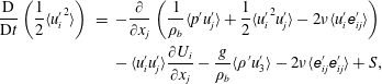 $$\begin{eqnarray}\displaystyle \frac{\text{D}}{\text{D}t}\left(\frac{1}{2}\langle {u_{i}^{\prime }}^{2}\rangle \right) & = & \displaystyle -\frac{\unicode[STIX]{x2202}}{\unicode[STIX]{x2202}x_{j}}\left(\frac{1}{\unicode[STIX]{x1D70C}_{b}}\langle p^{\prime }u_{j}^{\prime }\rangle +\frac{1}{2}\langle {u_{i}^{\prime }}^{2}u_{j}^{\prime }\rangle -2\unicode[STIX]{x1D708}\langle u_{i}^{\prime }\unicode[STIX]{x1D626}_{ij}^{\prime }\rangle \right)\nonumber\\ \displaystyle & & \displaystyle -\,\langle u_{i}^{\prime }u_{j}^{\prime }\rangle \frac{\unicode[STIX]{x2202}U_{i}}{\unicode[STIX]{x2202}x_{j}}-\frac{g}{\unicode[STIX]{x1D70C}_{b}}\langle \unicode[STIX]{x1D70C}^{\prime }u_{3}^{\prime }\rangle -2\unicode[STIX]{x1D708}\langle \unicode[STIX]{x1D626}_{ij}^{\prime }\unicode[STIX]{x1D626}_{ij}^{\prime }\rangle +S,\end{eqnarray}$$
where
 $g$
is gravity,
$g$
is gravity,
 $\unicode[STIX]{x1D708}$
is the kinematic viscosity of water,
$\unicode[STIX]{x1D708}$
is the kinematic viscosity of water,
 $\text{D}/\text{D}t\equiv \unicode[STIX]{x2202}/\unicode[STIX]{x2202}t+U_{j}(\unicode[STIX]{x2202}/\unicode[STIX]{x2202}x_{j})$
and the turbulent strain tensor,
$\text{D}/\text{D}t\equiv \unicode[STIX]{x2202}/\unicode[STIX]{x2202}t+U_{j}(\unicode[STIX]{x2202}/\unicode[STIX]{x2202}x_{j})$
and the turbulent strain tensor,
 $\unicode[STIX]{x1D626}_{ij}^{\prime }$
, is:
$\unicode[STIX]{x1D626}_{ij}^{\prime }$
, is:
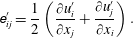 $$\begin{eqnarray}\unicode[STIX]{x1D626}_{ij}^{\prime }=\frac{1}{2}\left(\frac{\unicode[STIX]{x2202}u_{i}^{\prime }}{\unicode[STIX]{x2202}x_{j}}+\frac{\unicode[STIX]{x2202}u_{j}^{\prime }}{\unicode[STIX]{x2202}x_{i}}\right).\end{eqnarray}$$
The left-hand side of (4.1) is the total rate of change of mean TKE. The first three terms on the right-hand side of the equation are spatial transport of mean TKE. The fourth term is shear production of mean TKE. The fifth term is the buoyancy production or destruction of mean TKE from the density fluctuations. The sixth term is the viscous dissipation of mean TKE and
 $S$
is a source term that is attributed to the rainfall. Here, since the rain is falling on an initially quiescent water body and in the absence of wind, there is no mean flow (i.e.
$S$
is a source term that is attributed to the rainfall. Here, since the rain is falling on an initially quiescent water body and in the absence of wind, there is no mean flow (i.e.
 $U_{i}=0$
), and we expect the advection, and shear production, of turbulence to be negligible. Also, since the flow is axisymmetric, only the vertical transport of TKE might play a role but the near isotropy shown in figure 9 suggests that this term is small. Thus, apart from the source term
$U_{i}=0$
), and we expect the advection, and shear production, of turbulence to be negligible. Also, since the flow is axisymmetric, only the vertical transport of TKE might play a role but the near isotropy shown in figure 9 suggests that this term is small. Thus, apart from the source term
 $S$
, the terms remaining are the viscous dissipation:
$S$
, the terms remaining are the viscous dissipation:
 $$\begin{eqnarray}\unicode[STIX]{x1D700}=-2\unicode[STIX]{x1D708}\langle \unicode[STIX]{x1D626}_{ij}^{\prime }\unicode[STIX]{x1D626}_{ij}^{\prime }\rangle ,\end{eqnarray}$$
and the mean turbulent buoyancy flux term,
 $B_{t}$
, is:
$B_{t}$
, is:
 $$\begin{eqnarray}B_{t}=-\frac{g}{\unicode[STIX]{x1D70C}_{b}}\langle \unicode[STIX]{x1D70C}^{\prime }u_{3}^{\prime }\rangle .\end{eqnarray}$$
To estimate a volumetric dissipation rate, we have used the axisymmetric properties of the flow (Xu & Chen Reference Xu and Chen2013) and parametrized the terms in (4.3) not directly measured by our two-dimensional PIV system.
Figure 11(a) shows
 $\overline{\unicode[STIX]{x1D700}}$
, the time averaged profiles of
$\overline{\unicode[STIX]{x1D700}}$
, the time averaged profiles of
 $\unicode[STIX]{x1D700}$
for
$\unicode[STIX]{x1D700}$
for
 $180\leqslant t<300~\text{s}$
. Below
$180\leqslant t<300~\text{s}$
. Below
 $r_{c}$
, the profiles decrease monotonically and show that the levels of dissipation are weakly dependent on rain rates. It is important to note here that dissipation measurements using (4.3) and PIV data generally underestimate the dissipation because of the limited spatial resolution of the data. For example, given the spatial resolution of our measurements, we suppose that we can resolve approximately 30 %–70 % of
$r_{c}$
, the profiles decrease monotonically and show that the levels of dissipation are weakly dependent on rain rates. It is important to note here that dissipation measurements using (4.3) and PIV data generally underestimate the dissipation because of the limited spatial resolution of the data. For example, given the spatial resolution of our measurements, we suppose that we can resolve approximately 30 %–70 % of
 $\unicode[STIX]{x1D700}$
if the actual dissipation rate were
$\unicode[STIX]{x1D700}$
if the actual dissipation rate were
 $O(10^{-4}){-}O(10^{-5})$
(Lavoie et al.
Reference Lavoie, Avallone, De Gregorio, Romano and Antonia2007; de Jong et al.
Reference de Jong, Cao, Woodward, Salazar, Collins and Meng2008; Xu & Chen Reference Xu and Chen2013). In fact, we can estimate that our measurements capture fluid motions down to the Kolmogorov scale
$O(10^{-4}){-}O(10^{-5})$
(Lavoie et al.
Reference Lavoie, Avallone, De Gregorio, Romano and Antonia2007; de Jong et al.
Reference de Jong, Cao, Woodward, Salazar, Collins and Meng2008; Xu & Chen Reference Xu and Chen2013). In fact, we can estimate that our measurements capture fluid motions down to the Kolmogorov scale
 $\unicode[STIX]{x1D702}_{K}=(\unicode[STIX]{x1D708}^{3}\unicode[STIX]{x1D700}^{-1})^{1/4}$
for dissipation rates
$\unicode[STIX]{x1D702}_{K}=(\unicode[STIX]{x1D708}^{3}\unicode[STIX]{x1D700}^{-1})^{1/4}$
for dissipation rates
 $\unicode[STIX]{x1D700}\lessapprox 3\times 10^{-5}$
. At the other end of the eddy size spectrum, the largest eddies in the flow are expected to scale with the cavity radius
$\unicode[STIX]{x1D700}\lessapprox 3\times 10^{-5}$
. At the other end of the eddy size spectrum, the largest eddies in the flow are expected to scale with the cavity radius
 $r_{c}$
which is much smaller than our PIV field of view. Thus, for
$r_{c}$
which is much smaller than our PIV field of view. Thus, for
 $\unicode[STIX]{x1D700}\lessapprox 3\times 10^{-5}$
, our PIV measurements resolve all scales of the fluid motion from the largest anticipated eddy sizes, of order
$\unicode[STIX]{x1D700}\lessapprox 3\times 10^{-5}$
, our PIV measurements resolve all scales of the fluid motion from the largest anticipated eddy sizes, of order
 $O(r_{c})$
, and down to the Kolmogorov scale. Therefore, direct estimates of the dissipation using (4.3) provide accurate measures of the dissipation rates up to
$O(r_{c})$
, and down to the Kolmogorov scale. Therefore, direct estimates of the dissipation using (4.3) provide accurate measures of the dissipation rates up to
 $O(10^{-5})$
. In turn, this also means that the scales at which energy in generated and that at which it is dissipated are physically close, meaning that no well-developed inertial subrange can be expected in the turbulent spectrum and that dissipation cannot be evaluated using the inertial subrange. This is discussed by Peirson et al. (Reference Peirson, Beya, Banner, Peral and Azarmsa2013).
$O(10^{-5})$
. In turn, this also means that the scales at which energy in generated and that at which it is dissipated are physically close, meaning that no well-developed inertial subrange can be expected in the turbulent spectrum and that dissipation cannot be evaluated using the inertial subrange. This is discussed by Peirson et al. (Reference Peirson, Beya, Banner, Peral and Azarmsa2013).

Figure 11. Time averages of (a) the mean turbulent kinetic energy dissipation
 $\overline{\unicode[STIX]{x1D700}}$
and (b) the turbulent buoyancy flux
$\overline{\unicode[STIX]{x1D700}}$
and (b) the turbulent buoyancy flux
 $\overline{B_{t}}$
for
$\overline{B_{t}}$
for
 $180\leqslant t<300~\text{s}$
. Turbulent kinetic energy is produced (respectively destroyed) by buoyancy where
$180\leqslant t<300~\text{s}$
. Turbulent kinetic energy is produced (respectively destroyed) by buoyancy where
 $\overline{B_{t}}>0$
(respectively
$\overline{B_{t}}>0$
(respectively
 $\overline{B_{t}}<0$
). Above the depth of the cavity
$\overline{B_{t}}<0$
). Above the depth of the cavity
 $r_{c}$
the data obtained with PIV do not resolve the rapid motion and the velocity associated with the cavity formation and collapse. These data are likely underestimated and therefore presented here in light grey (see § 2.3.1). The faded symbol in (a) are excluded from the depth average shown in figure 12.
$r_{c}$
the data obtained with PIV do not resolve the rapid motion and the velocity associated with the cavity formation and collapse. These data are likely underestimated and therefore presented here in light grey (see § 2.3.1). The faded symbol in (a) are excluded from the depth average shown in figure 12.
Figure 11(b) shows
 $\overline{B_{t}}$
, the time averaged profiles of
$\overline{B_{t}}$
, the time averaged profiles of
 $B_{t}$
for
$B_{t}$
for
 $180\leqslant t<300~\text{s}$
. Here
$180\leqslant t<300~\text{s}$
. Here
 $B_{t}$
was computed using the
$B_{t}$
was computed using the
 $\unicode[STIX]{x1D70C}^{\prime }$
fields derived from the LIF. Because of laser light reflections from the surface and the associated focusing and defocusing caused by the surface disturbances (i.e. the ring waves caused by the rain and the surface cavities), the LIF was considered to be potentially contaminated in the near-surface region. Careful manual inspection of the LIF images revealed that the near-surface region where LIF could be contaminated is approximately as deep as twice the laser light sheet thickness. Consequently, the profiles of
$\unicode[STIX]{x1D70C}^{\prime }$
fields derived from the LIF. Because of laser light reflections from the surface and the associated focusing and defocusing caused by the surface disturbances (i.e. the ring waves caused by the rain and the surface cavities), the LIF was considered to be potentially contaminated in the near-surface region. Careful manual inspection of the LIF images revealed that the near-surface region where LIF could be contaminated is approximately as deep as twice the laser light sheet thickness. Consequently, the profiles of
 $\overline{B_{t}}$
shown in figure 11(b) only extend up to
$\overline{B_{t}}$
shown in figure 11(b) only extend up to
 $z=6~\text{mm}$
. For the purpose of the estimates presented here, this is not debilitating because, as mentioned above, our velocity measurements above
$z=6~\text{mm}$
. For the purpose of the estimates presented here, this is not debilitating because, as mentioned above, our velocity measurements above
 $r_{c}$
are likely underestimated. The profiles of
$r_{c}$
are likely underestimated. The profiles of
 $\overline{B_{t}}$
are predominantly positive for
$\overline{B_{t}}$
are predominantly positive for
 $R$
of 40 and
$R$
of 40 and
 $100~\text{mm}~\text{h}^{-1}$
indicating that there is buoyant production of turbulent kinetic energy. Conversely, the profile of
$100~\text{mm}~\text{h}^{-1}$
indicating that there is buoyant production of turbulent kinetic energy. Conversely, the profile of
 $\overline{B_{t}}$
is negative for
$\overline{B_{t}}$
is negative for
 $R$
of
$R$
of
 $190~\text{mm}~\text{h}^{-1}$
indicating that there is destruction of turbulent kinetic energy.
$190~\text{mm}~\text{h}^{-1}$
indicating that there is destruction of turbulent kinetic energy.
When averaged both in time and space (from
 $z=-15~\text{cm}$
to
$z=-15~\text{cm}$
to
 $z=r_{c}~\text{mm}$
), the mean turbulent energy dissipation
$z=r_{c}~\text{mm}$
), the mean turbulent energy dissipation
 $\overline{[\unicode[STIX]{x1D700}]}$
increases with rain rate between
$\overline{[\unicode[STIX]{x1D700}]}$
increases with rain rate between
 $R=40~\text{mm}~\text{h}^{-1}$
and
$R=40~\text{mm}~\text{h}^{-1}$
and
 $R=100~\text{mm}~\text{h}^{-1}$
but decreases substantially for
$R=100~\text{mm}~\text{h}^{-1}$
but decreases substantially for
 $R=190~\text{mm}~\text{h}^{-1}$
, similarly to
$R=190~\text{mm}~\text{h}^{-1}$
, similarly to
 $\overline{KE_{t}}$
shown on figure 10. Meanwhile, the mean turbulent buoyancy flux decreases with rain rate until it becomes negative for
$\overline{KE_{t}}$
shown on figure 10. Meanwhile, the mean turbulent buoyancy flux decreases with rain rate until it becomes negative for
 $R=190~\text{mm}~\text{h}^{-1}$
(figure 12). This regime change from buoyant production to buoyant destruction of turbulent kinetic energy at high rain rates may explain the reduction of turbulent kinetic energy shown in figure 10 and the decrease in dissipation (figure 12) at the highest rain rate. However, reliable density measurements and
$R=190~\text{mm}~\text{h}^{-1}$
(figure 12). This regime change from buoyant production to buoyant destruction of turbulent kinetic energy at high rain rates may explain the reduction of turbulent kinetic energy shown in figure 10 and the decrease in dissipation (figure 12) at the highest rain rate. However, reliable density measurements and
 $\overline{B_{t}}$
estimate are unavailable close to the interface (approximately within
$\overline{B_{t}}$
estimate are unavailable close to the interface (approximately within
 $r_{c}$
of the interface). At this point, the data suggest that the buoyancy induced by the mass flux from the rain eventually overrides the mixing efficiency of the turbulent kinetic energy flux from the rain, but the limited amount of data presented here dictates caution in making definitive deductions.
$r_{c}$
of the interface). At this point, the data suggest that the buoyancy induced by the mass flux from the rain eventually overrides the mixing efficiency of the turbulent kinetic energy flux from the rain, but the limited amount of data presented here dictates caution in making definitive deductions.

Figure 12. (a) Average turbulent kinetic energy dissipation
 $\overline{[\unicode[STIX]{x1D700}]}$
, and (b) average turbulent buoyancy production
$\overline{[\unicode[STIX]{x1D700}]}$
, and (b) average turbulent buoyancy production
 $\overline{[B_{t}]}$
.
$\overline{[B_{t}]}$
.
4.2 Kinetic energy flux from the rain
One remaining question has to do with the difference between the available energy from the rainfall and that measured in the subsurface turbulence as shown in (figure 9). Indeed, the kinetic energy from the rain fluxed through the surface is
 $KEF_{r}=(\unicode[STIX]{x1D70C}_{r}|\boldsymbol{v}_{I}|^{2}R)/2$
. With
$KEF_{r}=(\unicode[STIX]{x1D70C}_{r}|\boldsymbol{v}_{I}|^{2}R)/2$
. With
 $R$
ranging from 40 to
$R$
ranging from 40 to
 $190~\text{mm}~\text{h}^{-1}$
,
$190~\text{mm}~\text{h}^{-1}$
,
 $KEF_{r}$
is of the order of
$KEF_{r}$
is of the order of
 $2.7\times 10^{-1}$
, to
$2.7\times 10^{-1}$
, to
 $12.8\times 10^{-1}~\text{kg}~\text{s}^{-3}$
. Liow (Reference Liow2001) estimated that approximately 30 % of the kinetic energy available from the drops were lost to the generation of the impact crater. Assuming that the remaining kinetic energy is dissipated by the turbulence in a layer of depth
$12.8\times 10^{-1}~\text{kg}~\text{s}^{-3}$
. Liow (Reference Liow2001) estimated that approximately 30 % of the kinetic energy available from the drops were lost to the generation of the impact crater. Assuming that the remaining kinetic energy is dissipated by the turbulence in a layer of depth
 $h_{r}$
(Manton Reference Manton1973; Houk & Green Reference Houk and Green1976; Nystuen Reference Nystuen1990; Craeye Reference Craeye1998), (see Harrison et al.
Reference Harrison, Veron, Ho, Reid, Orton and McGillis2012), we can anticipate dissipation rates
$h_{r}$
(Manton Reference Manton1973; Houk & Green Reference Houk and Green1976; Nystuen Reference Nystuen1990; Craeye Reference Craeye1998), (see Harrison et al.
Reference Harrison, Veron, Ho, Reid, Orton and McGillis2012), we can anticipate dissipation rates
 $D_{\unicode[STIX]{x1D700},r}\approx 0.7(KEF_{r}/\unicode[STIX]{x1D70C}_{b}h_{r})$
of the order of
$D_{\unicode[STIX]{x1D700},r}\approx 0.7(KEF_{r}/\unicode[STIX]{x1D70C}_{b}h_{r})$
of the order of
 $1.7\times 10^{-2}$
, to
$1.7\times 10^{-2}$
, to
 $8.1\times 10^{-2}~\text{m}^{2}~\text{s}^{-3}$
if
$8.1\times 10^{-2}~\text{m}^{2}~\text{s}^{-3}$
if
 $h_{r}\approx r_{c}\approx 10^{-2}~\text{m}$
, or
$h_{r}\approx r_{c}\approx 10^{-2}~\text{m}$
, or
 $1.8\times 10^{-3}$
, to
$1.8\times 10^{-3}$
, to
 $8.8\times 10^{-3}~\text{m}^{2}~\text{s}^{-3}$
if
$8.8\times 10^{-3}~\text{m}^{2}~\text{s}^{-3}$
if
 $h_{r}$
is
$h_{r}$
is
 $O(10^{-1})~\text{m}$
(Green & Houk Reference Green and Houk1979; Braun Reference Braun2003; Beya et al.
Reference Beya, Peirson, Banner, Komori, McGillis and Kurose2011; Harrison et al.
Reference Harrison, Veron, Ho, Reid, Orton and McGillis2012; Peirson et al.
Reference Peirson, Beya, Banner, Peral and Azarmsa2013). But looking at the data of figures 11 and 12, at depth
$O(10^{-1})~\text{m}$
(Green & Houk Reference Green and Houk1979; Braun Reference Braun2003; Beya et al.
Reference Beya, Peirson, Banner, Komori, McGillis and Kurose2011; Harrison et al.
Reference Harrison, Veron, Ho, Reid, Orton and McGillis2012; Peirson et al.
Reference Peirson, Beya, Banner, Peral and Azarmsa2013). But looking at the data of figures 11 and 12, at depth
 $z\approx r_{c}$
,
$z\approx r_{c}$
,
 $\overline{\unicode[STIX]{x1D700}}$
is
$\overline{\unicode[STIX]{x1D700}}$
is
 $O(10^{-5})~\text{m}^{2}~\text{s}^{-3}$
(figure 11). Alternatively, when integrated over depth of
$O(10^{-5})~\text{m}^{2}~\text{s}^{-3}$
(figure 11). Alternatively, when integrated over depth of
 $O(10^{-1})~\text{m}$
,
$O(10^{-1})~\text{m}$
,
 $\overline{[\unicode[STIX]{x1D700}]}$
is
$\overline{[\unicode[STIX]{x1D700}]}$
is
 $O(10^{-6})~\text{m}^{2}~\text{s}^{-3}$
(figure 12). In either case, the measured dissipation rates are approximately 0.1 %–0.3 % of that estimated from the kinetic energy flux available from the rainfall. This is in agreement with the results of Beya et al. (Reference Beya, Peirson, Banner, Komori, McGillis and Kurose2011) who found, by estimating the dissipation from inertial scaling, that dissipation accounted for 0.2 % of the rainfall energy. The results of Beya et al. (Reference Beya, Peirson, Banner, Komori, McGillis and Kurose2011) and that presented here suggest that the bulk of the kinetic energy from rainfall is dissipated at shallow depth not resolved here or transferred to other phenomena. In fact, based on further analysis of the data set of Beya et al. (Reference Beya, Peirson, Banner, Komori, McGillis and Kurose2011), Peirson et al. (Reference Peirson, Beya, Banner, Peral and Azarmsa2013) had indeed concluded that ‘significant dissipation occurs in the vicinity of the open water surface’.
$O(10^{-6})~\text{m}^{2}~\text{s}^{-3}$
(figure 12). In either case, the measured dissipation rates are approximately 0.1 %–0.3 % of that estimated from the kinetic energy flux available from the rainfall. This is in agreement with the results of Beya et al. (Reference Beya, Peirson, Banner, Komori, McGillis and Kurose2011) who found, by estimating the dissipation from inertial scaling, that dissipation accounted for 0.2 % of the rainfall energy. The results of Beya et al. (Reference Beya, Peirson, Banner, Komori, McGillis and Kurose2011) and that presented here suggest that the bulk of the kinetic energy from rainfall is dissipated at shallow depth not resolved here or transferred to other phenomena. In fact, based on further analysis of the data set of Beya et al. (Reference Beya, Peirson, Banner, Komori, McGillis and Kurose2011), Peirson et al. (Reference Peirson, Beya, Banner, Peral and Azarmsa2013) had indeed concluded that ‘significant dissipation occurs in the vicinity of the open water surface’.
To explore suite of phenomena occurring during rain impact, we turn to the large body of detailed work on single drop impacts on liquid pools. As noted in the introduction, since the pioneering work of Worthington & Cole (Reference Worthington and Cole1897), Worthington (Reference Worthington1908) on the impact dynamics on deep liquid films, there has been a large amount of work on single drop impacts on liquid and solid surfaces, most of it motivated by industrial application such as cooling and surface coating (see Yarin Reference Yarin2006). The dynamics of the impact includes bouncing, coalescence, generation of crater, crowns splash, jet splash and bubble entrainment (e.g. Jayaratne & Mason Reference Jayaratne and Mason1964; Chapman & Critchlow Reference Chapman and Critchlow1967; Ching, Golay & Johnson Reference Ching, Golay and Johnson1984; Rodriguez & Mesler Reference Rodriguez and Mesler1988; Cai Reference Cai1989; Rein Reference Rein1993; Peck & Sigurdson Reference Peck and Sigurdson1994; Cresswell & Morton Reference Cresswell and Morton1995; Shankar & Kumar Reference Shankar and Kumar1995; Rein Reference Rein1996; Dooley et al.
Reference Dooley, Warncke, Gharib and Tryggvason1997; Morton et al.
Reference Morton, Rudman and Liow2000; Liow Reference Liow2001; Fedorchenko & Wang Reference Fedorchenko and Wang2004; Vander Wal, Berger & Mozes Reference Vander Wal, Berger and Mozes2006; Cole Reference Cole2007; Ray, Biswas & Sharma Reference Ray, Biswas and Sharma2010; Takagaki & Komori Reference Takagaki and Komori2014; Ray et al.
Reference Ray, Biswas and Sharma2015; San Lee et al.
Reference San Lee, Park, Lee, Weon, Fezzaa and Je2015). All the impact-related phenomena are reasonably well parametrized using the impact Weber number (
 $We=\unicode[STIX]{x1D70C}_{r}|\boldsymbol{v}_{I}|^{2}2r/\unicode[STIX]{x1D6E4}$
), and Froude number (
$We=\unicode[STIX]{x1D70C}_{r}|\boldsymbol{v}_{I}|^{2}2r/\unicode[STIX]{x1D6E4}$
), and Froude number (
 $Fr=|\boldsymbol{v}_{I}|^{2}/(2gr)$
), with
$Fr=|\boldsymbol{v}_{I}|^{2}/(2gr)$
), with
 $\unicode[STIX]{x1D6E4}$
the surface tension. While the data of Engel (Reference Engel1966) and Liow (Reference Liow2001) suggest that approximately 30 % of the kinetic energy available from the drops was lost to the generation of the impact crater, the data of Cai (Reference Cai1989) and Pumphrey & Crum (Reference Pumphrey and Crum1990) suggest that up to 90 % of the rain kinetic energy could be spent on the generation of the crater. Rein (Reference Rein1996) also noted that the vortex ring shed by a single drop impact contained about 5 % of the impact energy, but he noted that less energy is contained in the vortex ring when the impact dynamics leads to the formation of craters. His results, as well as that of Cai (Reference Cai1989) and Pumphrey & Crum (Reference Pumphrey and Crum1990) were obtained for significantly lower impact Froude numbers that those of the experiments presented here.
$\unicode[STIX]{x1D6E4}$
the surface tension. While the data of Engel (Reference Engel1966) and Liow (Reference Liow2001) suggest that approximately 30 % of the kinetic energy available from the drops was lost to the generation of the impact crater, the data of Cai (Reference Cai1989) and Pumphrey & Crum (Reference Pumphrey and Crum1990) suggest that up to 90 % of the rain kinetic energy could be spent on the generation of the crater. Rein (Reference Rein1996) also noted that the vortex ring shed by a single drop impact contained about 5 % of the impact energy, but he noted that less energy is contained in the vortex ring when the impact dynamics leads to the formation of craters. His results, as well as that of Cai (Reference Cai1989) and Pumphrey & Crum (Reference Pumphrey and Crum1990) were obtained for significantly lower impact Froude numbers that those of the experiments presented here.
The vortex rings associated with drop impacts, which are beautifully depicted in the paper of Peck & Sigurdson (Reference Peck and Sigurdson1994), are believed to be associated with the generation of vorticity as the drop coalesces with the receiving liquid. But coalescence, and thus vortex ring formation occurs at
 $We<O(50{-}100)$
, below the so-called regular bubble entrainment regime (Oguz & Prosperetti Reference Oguz and Prosperetti1990). Here, and for large drops in natural rainfall, the impacts are in the splashing regime where few, if any, vortex rings are expected. This is consistent with our results which overall show only occasional clear vortex ring penetration in the fluid. See figure 8 where we can clearly count
$We<O(50{-}100)$
, below the so-called regular bubble entrainment regime (Oguz & Prosperetti Reference Oguz and Prosperetti1990). Here, and for large drops in natural rainfall, the impacts are in the splashing regime where few, if any, vortex rings are expected. This is consistent with our results which overall show only occasional clear vortex ring penetration in the fluid. See figure 8 where we can clearly count
 $O(10)$
high TKE event associated with the penetration of individual vortices, whereas we expect, based on rain rates,
$O(10)$
high TKE event associated with the penetration of individual vortices, whereas we expect, based on rain rates,
 $O(100)$
rain drop impacts in the PIV field of view.
$O(100)$
rain drop impacts in the PIV field of view.
At
 $We\approx O(300)$
, Morton et al. (Reference Morton, Rudman and Liow2000) showed, in numerical simulations, that vortex rings can still be generated. In very recent numerical work Ray et al. (Reference Ray, Biswas and Sharma2015) show similar results with vortex rings up to
$We\approx O(300)$
, Morton et al. (Reference Morton, Rudman and Liow2000) showed, in numerical simulations, that vortex rings can still be generated. In very recent numerical work Ray et al. (Reference Ray, Biswas and Sharma2015) show similar results with vortex rings up to
 $We\approx O(300)$
. This was recently confirmed by San Lee et al. (Reference San Lee, Park, Lee, Weon, Fezzaa and Je2015) who indeed showed experimentally the existence of that small vortices generated for
$We\approx O(300)$
. This was recently confirmed by San Lee et al. (Reference San Lee, Park, Lee, Weon, Fezzaa and Je2015) who indeed showed experimentally the existence of that small vortices generated for
 $We>64$
. In all cases, these vortices occurred at sub-millimetre scales and were trapped near the surface. Takagaki & Komori (Reference Takagaki and Komori2014) also observed vortices which they dubbed ‘water column vortices’ that occurred after a high
$We>64$
. In all cases, these vortices occurred at sub-millimetre scales and were trapped near the surface. Takagaki & Komori (Reference Takagaki and Komori2014) also observed vortices which they dubbed ‘water column vortices’ that occurred after a high
 $Fr$
impact but were actually generated by the coalescence (or collapse) of the stalk.
$Fr$
impact but were actually generated by the coalescence (or collapse) of the stalk.

Figure 13.
 $Fr$
–
$Fr$
–
 $We$
parameter space graph showing different drop impact regimes. The approximate regimes for coalescing, floating and bouncing drops are separated with grey dashed lines. The black dash lines
$We$
parameter space graph showing different drop impact regimes. The approximate regimes for coalescing, floating and bouncing drops are separated with grey dashed lines. The black dash lines
 $Fr^{1/4}$
and
$Fr^{1/4}$
and
 $Fr^{1/5}$
show regimes where bubble entrainment is observed. The solid black line shows rainfall terminal velocity along with the drop radius (black) and the impact velocity
$Fr^{1/5}$
show regimes where bubble entrainment is observed. The solid black line shows rainfall terminal velocity along with the drop radius (black) and the impact velocity
 $|\boldsymbol{v}_{I}|$
(grey in parenthesis). The solid black circle shows
$|\boldsymbol{v}_{I}|$
(grey in parenthesis). The solid black circle shows
 $Fr$
and
$Fr$
and
 $We$
for these experiments. (Adapted from Liow Reference Liow2001).
$We$
for these experiments. (Adapted from Liow Reference Liow2001).
We note again that the overwhelming majority of previous work was done with single drop impact on flat and quiescent interfaces and without buoyancy effects. Under natural rainfall, a drop impacts an already disturbed surface where the subsurface flow is already turbulent. It is doubtful that stable, long-lived vortex rings form under these conditions. Again, this is corroborated by the less-than-expected number of intense vortices visible in figure 8. It is also likely that the surface geometry substantially modifies the impact dynamics (see below). Furthermore, most the work cited above was also performed at modest
 $Fr$
and
$Fr$
and
 $We$
.
$We$
.
In other words, there are very little data available for impacts representative of natural rainfall at terminal velocity which systematically falls in the large Froude number regime. For perspective, figure 13 shows the
 $Fr$
–
$Fr$
–
 $We$
parameter space diagram adapted from Liow (Reference Liow2001) and highlights some of the available data. Natural rainfall conditions are infrequently studied, if at all. For example, the recent data set of Peirson et al. (Reference Peirson, Beya, Banner, Peral and Azarmsa2013) on the effect of rain-generated turbulence on surface waves and wave damping, falls short of impact Froude numbers from natural rainfall. This is in part due to the difficulty associated with achieving terminal fall velocities in a confined laboratory space. We note here that Engel (Reference Engel1966) achieved hyper-terminal velocity in the laboratory by having water drop fall in tubes where air pressure, and thus drag, was significantly reduced. The results of Engel (Reference Engel1966) are not included in figure 13. We also note that taking the results of Cai (Reference Cai1989) and Pumphrey & Crum (Reference Pumphrey and Crum1990) and estimating
$We$
parameter space diagram adapted from Liow (Reference Liow2001) and highlights some of the available data. Natural rainfall conditions are infrequently studied, if at all. For example, the recent data set of Peirson et al. (Reference Peirson, Beya, Banner, Peral and Azarmsa2013) on the effect of rain-generated turbulence on surface waves and wave damping, falls short of impact Froude numbers from natural rainfall. This is in part due to the difficulty associated with achieving terminal fall velocities in a confined laboratory space. We note here that Engel (Reference Engel1966) achieved hyper-terminal velocity in the laboratory by having water drop fall in tubes where air pressure, and thus drag, was significantly reduced. The results of Engel (Reference Engel1966) are not included in figure 13. We also note that taking the results of Cai (Reference Cai1989) and Pumphrey & Crum (Reference Pumphrey and Crum1990) and estimating
 $D_{\unicode[STIX]{x1D700},r}$
assuming that 90 % (instead of 30 %) of the rain kinetic energy is spent on the generation of the crater, leads to
$D_{\unicode[STIX]{x1D700},r}$
assuming that 90 % (instead of 30 %) of the rain kinetic energy is spent on the generation of the crater, leads to
 $D_{\unicode[STIX]{x1D700},r}$
being approximately
$D_{\unicode[STIX]{x1D700},r}$
being approximately
 $O(100)$
times larger than the measured dissipation rates. The difference with the estimate of Beya et al. (Reference Beya, Peirson, Banner, Komori, McGillis and Kurose2011) is an order of magnitude larger (because they did not account for the energy lost to the crater formation) but the inference that the bulk of the kinetic energy from rainfall is dissipated by mechanisms at scaled not yet resolved, remains. We suggest that surface trapped, sub-millimetre scale vortices recently observed by (San Lee et al.
Reference San Lee, Park, Lee, Weon, Fezzaa and Je2015) and un-resolved in our experiments, may serve to dissipate a substantial fraction of the impact kinetic energy. It is also likely that the dynamics involved in the crown and splash formation, both of which involve scales where capillary forces cannot be neglected, may serve to dissipate significant amount of energy.
$O(100)$
times larger than the measured dissipation rates. The difference with the estimate of Beya et al. (Reference Beya, Peirson, Banner, Komori, McGillis and Kurose2011) is an order of magnitude larger (because they did not account for the energy lost to the crater formation) but the inference that the bulk of the kinetic energy from rainfall is dissipated by mechanisms at scaled not yet resolved, remains. We suggest that surface trapped, sub-millimetre scale vortices recently observed by (San Lee et al.
Reference San Lee, Park, Lee, Weon, Fezzaa and Je2015) and un-resolved in our experiments, may serve to dissipate a substantial fraction of the impact kinetic energy. It is also likely that the dynamics involved in the crown and splash formation, both of which involve scales where capillary forces cannot be neglected, may serve to dissipate significant amount of energy.
4.3 Turbulent length scales
In a further attempt to better understand the discrepancy outlined above, we estimate, assuming isotropic turbulence (Lesieur Reference Lesieur2008), the Taylor microscale,
 $\unicode[STIX]{x1D706}_{T}$
, derived from the velocity correlation:
$\unicode[STIX]{x1D706}_{T}$
, derived from the velocity correlation:
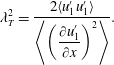 $$\begin{eqnarray}\unicode[STIX]{x1D706}_{T}^{2}=\frac{2\langle u_{1}^{\prime }u_{1}^{\prime }\rangle }{\left\langle \left({\displaystyle \frac{\unicode[STIX]{x2202}u_{1}^{\prime }}{\unicode[STIX]{x2202}x}}\right)^{2}\right\rangle }.\end{eqnarray}$$
Figure 14 shows the average Taylor microscale
 $\overline{\unicode[STIX]{x1D706}_{T}}$
, averaged for times
$\overline{\unicode[STIX]{x1D706}_{T}}$
, averaged for times
 $180\leqslant t<300~\text{s}$
, and normalized by the crater depth
$180\leqslant t<300~\text{s}$
, and normalized by the crater depth
 $r_{c}$
. It is plotted as a function depth, also normalized by the crater depth. Figure 14 shows that the
$r_{c}$
. It is plotted as a function depth, also normalized by the crater depth. Figure 14 shows that the
 $\overline{\unicode[STIX]{x1D706}_{T}}$
scales with the crater depth and decays as
$\overline{\unicode[STIX]{x1D706}_{T}}$
scales with the crater depth and decays as
 $z^{-2/3}$
for
$z^{-2/3}$
for
 $z\geqslant 2r_{c}$
. These results are largely independent of rain rates. Since there is no wind and no wind waves present in the experimental cases presented here, it is indeed expected that the largest scales in the turbulence compare with the largest scales generated by the drop impact process, i.e. the scale of the impact crater and eventual vortex ring. However, the reader is reminded that the estimates of the Taylor microscale rely on assumptions of isotropy and a Kolmogorov-type spectrum, which may not be the case here where stratification is present and with a turbulent a regime for which an inertial subrange may not be well developed (see above and discussion in Peirson et al.
Reference Peirson, Beya, Banner, Peral and Azarmsa2013). Therefore, in this paper, we consider values of the Taylor microscale and quantities derived from it as useful ‘order of magnitude only’ estimations. For example, we further estimate the dissipation using:
$z\geqslant 2r_{c}$
. These results are largely independent of rain rates. Since there is no wind and no wind waves present in the experimental cases presented here, it is indeed expected that the largest scales in the turbulence compare with the largest scales generated by the drop impact process, i.e. the scale of the impact crater and eventual vortex ring. However, the reader is reminded that the estimates of the Taylor microscale rely on assumptions of isotropy and a Kolmogorov-type spectrum, which may not be the case here where stratification is present and with a turbulent a regime for which an inertial subrange may not be well developed (see above and discussion in Peirson et al.
Reference Peirson, Beya, Banner, Peral and Azarmsa2013). Therefore, in this paper, we consider values of the Taylor microscale and quantities derived from it as useful ‘order of magnitude only’ estimations. For example, we further estimate the dissipation using:
 $$\begin{eqnarray}\unicode[STIX]{x1D700}_{\unicode[STIX]{x1D706}_{T}}=15\unicode[STIX]{x1D708}\frac{\overline{\langle u_{1}^{\prime 2}\rangle }}{\unicode[STIX]{x1D706}_{T}^{2}}.\end{eqnarray}$$
From the data of figures 9 and 14, we thus estimate that
 $\unicode[STIX]{x1D700}_{\unicode[STIX]{x1D706}_{T}}$
is of order
$\unicode[STIX]{x1D700}_{\unicode[STIX]{x1D706}_{T}}$
is of order
 $15\unicode[STIX]{x1D708}(O(10^{-4})/O(10^{-4}))\approx 1.5\times 10^{-5}~\text{m}^{2}~\text{s}^{-3}$
for
$15\unicode[STIX]{x1D708}(O(10^{-4})/O(10^{-4}))\approx 1.5\times 10^{-5}~\text{m}^{2}~\text{s}^{-3}$
for
 $z\approx r_{c}$
. This is consistent with the results shown on figure 11 where
$z\approx r_{c}$
. This is consistent with the results shown on figure 11 where
 $\overline{\unicode[STIX]{x1D700}}\approx 2\times 10^{-5}~\text{m}^{2}~\text{s}^{-3}$
. At larger depth, our data suggest that
$\overline{\unicode[STIX]{x1D700}}\approx 2\times 10^{-5}~\text{m}^{2}~\text{s}^{-3}$
. At larger depth, our data suggest that
 $\overline{\langle u_{1}^{\prime 2}\rangle }\propto z^{-3}$
and
$\overline{\langle u_{1}^{\prime 2}\rangle }\propto z^{-3}$
and
 $\unicode[STIX]{x1D706}_{T}^{2}\propto z^{-4/3}$
suggesting that
$\unicode[STIX]{x1D706}_{T}^{2}\propto z^{-4/3}$
suggesting that
 $\unicode[STIX]{x1D700}_{\unicode[STIX]{x1D706}_{T}}\propto z^{-5/3}$
. For reference, we have plotted the
$\unicode[STIX]{x1D700}_{\unicode[STIX]{x1D706}_{T}}\propto z^{-5/3}$
. For reference, we have plotted the
 $z^{-5/3}$
dependence on figure 11.
$z^{-5/3}$
dependence on figure 11.

Figure 14. Average Taylor microscale profiles
 $\overline{\unicode[STIX]{x1D706}_{T}}$
as a function of rain rate. Above the depth of the cavity
$\overline{\unicode[STIX]{x1D706}_{T}}$
as a function of rain rate. Above the depth of the cavity
 $r_{c}$
the data obtained with PIV do not resolve the rapid motion and the velocity associated with the cavity formation and collapse. These data are likely underestimated and therefore presented here in light grey (see § 2.3.1).
$r_{c}$
the data obtained with PIV do not resolve the rapid motion and the velocity associated with the cavity formation and collapse. These data are likely underestimated and therefore presented here in light grey (see § 2.3.1).
4.4 Eddy viscosity
Several investigations of the damping of surface waves by rainfall have estimated the eddy viscosity,
 $\unicode[STIX]{x1D708}_{e}$
, near the surface (Tsimplis & Thorpe Reference Tsimplis and Thorpe1989; Poon et al.
Reference Poon, Tang and Wu1992; Tsimplis Reference Tsimplis1992; Braun Reference Braun2003; Harrison Reference Harrison2012; Peirson et al.
Reference Peirson, Beya, Banner, Peral and Azarmsa2013). These estimates utilized the changes in wave-height spectra as the waves propagate through a rain patch. However, Harrison (Reference Harrison2012) concluded that this method systematically underestimates
$\unicode[STIX]{x1D708}_{e}$
, near the surface (Tsimplis & Thorpe Reference Tsimplis and Thorpe1989; Poon et al.
Reference Poon, Tang and Wu1992; Tsimplis Reference Tsimplis1992; Braun Reference Braun2003; Harrison Reference Harrison2012; Peirson et al.
Reference Peirson, Beya, Banner, Peral and Azarmsa2013). These estimates utilized the changes in wave-height spectra as the waves propagate through a rain patch. However, Harrison (Reference Harrison2012) concluded that this method systematically underestimates
 $\unicode[STIX]{x1D708}_{e}$
because of the competing effects of rain-induced high-frequency wave generation and rain-induced wave damping. These competing effects render estimates of the functional form of
$\unicode[STIX]{x1D708}_{e}$
because of the competing effects of rain-induced high-frequency wave generation and rain-induced wave damping. These competing effects render estimates of the functional form of
 $\unicode[STIX]{x1D708}_{e}(z)$
difficult. Here, keeping in mind the limitations outlined above, we use the Taylor microscale once more and estimate the eddy viscosity using:
$\unicode[STIX]{x1D708}_{e}(z)$
difficult. Here, keeping in mind the limitations outlined above, we use the Taylor microscale once more and estimate the eddy viscosity using:
 $$\begin{eqnarray}\unicode[STIX]{x1D708}_{e}=\unicode[STIX]{x1D706}_{T}\overline{\langle u_{1}^{\prime 2}\rangle }^{1/2}.\end{eqnarray}$$
We find that
 $\unicode[STIX]{x1D708}_{e}$
is of
$\unicode[STIX]{x1D708}_{e}$
is of
 $O(10^{-4})~\text{m}^{2}~\text{s}^{-1}$
for
$O(10^{-4})~\text{m}^{2}~\text{s}^{-1}$
for
 $z\approx r_{c}$
and decreases to approximately
$z\approx r_{c}$
and decreases to approximately
 $3\times 10^{-5}~\text{m}^{2}~\text{s}^{-1}$
for
$3\times 10^{-5}~\text{m}^{2}~\text{s}^{-1}$
for
 $z\approx 10~\text{cm}$
. This is consistent with the diffusive estimate obtained from the flow visualization presented in § 3.1. We note here that estimating
$z\approx 10~\text{cm}$
. This is consistent with the diffusive estimate obtained from the flow visualization presented in § 3.1. We note here that estimating
 $\unicode[STIX]{x1D708}_{e}$
from the damping of the surface wave essentially integrates
$\unicode[STIX]{x1D708}_{e}$
from the damping of the surface wave essentially integrates
 $\unicode[STIX]{x1D708}_{e}(z)$
down to depth comparable with the surface wave wavelength. Measuring
$\unicode[STIX]{x1D708}_{e}(z)$
down to depth comparable with the surface wave wavelength. Measuring
 $\unicode[STIX]{x1D708}_{e}(z)$
for depth of order
$\unicode[STIX]{x1D708}_{e}(z)$
for depth of order
 $O(1)~\text{cm}$
would require the use of cm scale surface waves for which viscous damping becomes substantial. At these small scales, rain impact crater radii also approach the surface wave wavelength making experiments challenging if not questionable. This ‘depth integration’ is another reason why estimates of
$O(1)~\text{cm}$
would require the use of cm scale surface waves for which viscous damping becomes substantial. At these small scales, rain impact crater radii also approach the surface wave wavelength making experiments challenging if not questionable. This ‘depth integration’ is another reason why estimates of
 $\unicode[STIX]{x1D708}_{e}$
made from the damping of surface waves are likely to be an underestimate of what might be expected very close to the interface. Here, depth integrated eddy viscosities
$\unicode[STIX]{x1D708}_{e}$
made from the damping of surface waves are likely to be an underestimate of what might be expected very close to the interface. Here, depth integrated eddy viscosities
 $\overline{[\unicode[STIX]{x1D708}_{e}]}$
are found to be of order
$\overline{[\unicode[STIX]{x1D708}_{e}]}$
are found to be of order
 $8\times 10^{-5}~\text{m}^{2}~\text{s}^{-1}$
, i.e. larger (as expected) than the value
$8\times 10^{-5}~\text{m}^{2}~\text{s}^{-1}$
, i.e. larger (as expected) than the value
 $0.86\times 10^{-5}~\text{m}^{2}~\text{s}^{-1}$
reported by Peirson et al. (Reference Peirson, Beya, Banner, Peral and Azarmsa2013) but of the same order of magnitude as the results of Tsimplis & Thorpe (Reference Tsimplis and Thorpe1989), Poon et al. (Reference Poon, Tang and Wu1992), Tsimplis (Reference Tsimplis1992) and Braun (Reference Braun2003). We also expect the profile
$0.86\times 10^{-5}~\text{m}^{2}~\text{s}^{-1}$
reported by Peirson et al. (Reference Peirson, Beya, Banner, Peral and Azarmsa2013) but of the same order of magnitude as the results of Tsimplis & Thorpe (Reference Tsimplis and Thorpe1989), Poon et al. (Reference Poon, Tang and Wu1992), Tsimplis (Reference Tsimplis1992) and Braun (Reference Braun2003). We also expect the profile
 $\unicode[STIX]{x1D708}_{e}(z)$
to depend on buoyancy. Thus wave damping experiments and estimates of
$\unicode[STIX]{x1D708}_{e}(z)$
to depend on buoyancy. Thus wave damping experiments and estimates of
 $\unicode[STIX]{x1D708}_{e}$
are expected to yield different results in fresh or seawater, as observed by Harrison (Reference Harrison2012). Overall, the range of eddy diffusivity values previously reported span at least an order of magnitude. At this point, the usefulness of such parametrization to examine rain-induced turbulence and its effect might be limited. Further investigations into the details of rain-generated turbulence are needed.
$\unicode[STIX]{x1D708}_{e}$
are expected to yield different results in fresh or seawater, as observed by Harrison (Reference Harrison2012). Overall, the range of eddy diffusivity values previously reported span at least an order of magnitude. At this point, the usefulness of such parametrization to examine rain-induced turbulence and its effect might be limited. Further investigations into the details of rain-generated turbulence are needed.
4.5 Saturation of surface disturbance
In an attempt to explain the insensitivity of both the rain attenuation rates and the subsurface fluctuating velocity to the rain rate, Peirson et al. (Reference Peirson, Beya, Banner, Peral and Azarmsa2013) compared the surface renewal time scale calculated by Craeye (Reference Craeye1998) with time scales associated with drop impingement (Fedorchenko & Wang Reference Fedorchenko and Wang2004) and ring waves (Le Méhauté Reference Le Méhauté1988). They suggested that above rain rates of approximately
 $30~\text{mm}~\text{h}^{-1}$
, the surface becomes saturated such that ‘increasing the rainfall rate may merely increase the frequency of ricocheting or spallation motions with negligible increase in deeply penetrating vertical droplet motions’.
$30~\text{mm}~\text{h}^{-1}$
, the surface becomes saturated such that ‘increasing the rainfall rate may merely increase the frequency of ricocheting or spallation motions with negligible increase in deeply penetrating vertical droplet motions’.
This is an interesting proposition and we suggest here that the range at which this saturated regime appears can be formerly estimated. Indeed, the drop size distribution
 $n(r)$
(see distribution proposed by Marshall & Palmer (Reference Marshall and Palmer1948) for example) gives the number of rain drop (per cubic metre of air, per radius increment). Then
$n(r)$
(see distribution proposed by Marshall & Palmer (Reference Marshall and Palmer1948) for example) gives the number of rain drop (per cubic metre of air, per radius increment). Then
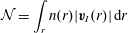 $$\begin{eqnarray}{\mathcal{N}}=\int _{r}n(r)|\boldsymbol{v}_{I}(r)|\,\text{d}r\end{eqnarray}$$
is the number flux of drop impacts (i.e. the number of impacts on the surface, per square metre per second). If we assume that each drop impact disturbs the surface for a duration
 $\hat{t}$
and over an area of radius
$\hat{t}$
and over an area of radius
 $\hat{r}$
, then the fraction of the interface disturbed by rainfall at any time is given by:
$\hat{r}$
, then the fraction of the interface disturbed by rainfall at any time is given by:
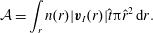 $$\begin{eqnarray}{\mathcal{A}}=\int _{r}n(r)|\boldsymbol{v}_{I}(r)|\hat{t}\unicode[STIX]{x03C0}\hat{r}^{2}\,\text{d}r.\end{eqnarray}$$
Thus, when
 ${\mathcal{A}}$
approaches unity, statistically, a drop is likely to fall at a location on the surface that is still disturbed under the effect of a previous impact.
${\mathcal{A}}$
approaches unity, statistically, a drop is likely to fall at a location on the surface that is still disturbed under the effect of a previous impact.
We can then estimate the rain rate at which
 ${\mathcal{A}}=1$
by simply choosing appropriate length scale
${\mathcal{A}}=1$
by simply choosing appropriate length scale
 $\hat{r}$
, and time scale
$\hat{r}$
, and time scale
 $\hat{t}$
. As an initial scaling attempt, we propose that the surface disturbed by a drop impact is propositional to the crater size
$\hat{t}$
. As an initial scaling attempt, we propose that the surface disturbed by a drop impact is propositional to the crater size
 $\hat{r}=\unicode[STIX]{x1D6FC}r_{c}$
, with
$\hat{r}=\unicode[STIX]{x1D6FC}r_{c}$
, with
 $\unicode[STIX]{x1D6FC}$
of order
$\unicode[STIX]{x1D6FC}$
of order
 $O(1{-}10)$
for example. Similarly, we suggest that the duration of the disturbance
$O(1{-}10)$
for example. Similarly, we suggest that the duration of the disturbance
 $\hat{t}$
, scales with the formation time of the crater
$\hat{t}$
, scales with the formation time of the crater
 $t_{c}=0.4(r_{c}/r)^{5/2}(r/|\boldsymbol{v}_{I}(r)|)$
(Liow Reference Liow2001), so that
$t_{c}=0.4(r_{c}/r)^{5/2}(r/|\boldsymbol{v}_{I}(r)|)$
(Liow Reference Liow2001), so that
 $\hat{t}=\unicode[STIX]{x1D6FD}t_{c}$
with
$\hat{t}=\unicode[STIX]{x1D6FD}t_{c}$
with
 $\unicode[STIX]{x1D6FD}$
also of order
$\unicode[STIX]{x1D6FD}$
also of order
 $O(1{-}10)$
. Taking the rain drop distribution of Marshall & Palmer (Reference Marshall and Palmer1948), and reasonable values of
$O(1{-}10)$
. Taking the rain drop distribution of Marshall & Palmer (Reference Marshall and Palmer1948), and reasonable values of
 $\unicode[STIX]{x1D6FC}=4$
and
$\unicode[STIX]{x1D6FC}=4$
and
 $\unicode[STIX]{x1D6FD}=5$
leads to a saturation regime starting at rain rates
$\unicode[STIX]{x1D6FD}=5$
leads to a saturation regime starting at rain rates
 $R\approx 35~\text{mm}~\text{h}^{-1}$
which is remarkably close to the estimate of Peirson et al. (Reference Peirson, Beya, Banner, Peral and Azarmsa2013). Evidently, with this simple scaling,
$R\approx 35~\text{mm}~\text{h}^{-1}$
which is remarkably close to the estimate of Peirson et al. (Reference Peirson, Beya, Banner, Peral and Azarmsa2013). Evidently, with this simple scaling,
 ${\mathcal{A}}\propto \unicode[STIX]{x1D6FC}^{2}\unicode[STIX]{x1D6FD}$
so robust estimates of
${\mathcal{A}}\propto \unicode[STIX]{x1D6FC}^{2}\unicode[STIX]{x1D6FD}$
so robust estimates of
 $\hat{r}$
and
$\hat{r}$
and
 $\hat{t}$
are necessary in order to narrow down the range of rain rates at which the surface may approach a saturated state. This saturation effect would also be exacerbated by the shift in
$\hat{t}$
are necessary in order to narrow down the range of rain rates at which the surface may approach a saturated state. This saturation effect would also be exacerbated by the shift in
 $n(r)$
to larger rain drops (larger
$n(r)$
to larger rain drops (larger
 $We$
at impact) with increasing rain rates. Therefore, increasing rain rates would increase the number of the rain drops in the splash regime and reduce the number of rain drops leading to the generation of vortex rings.
$We$
at impact) with increasing rain rates. Therefore, increasing rain rates would increase the number of the rain drops in the splash regime and reduce the number of rain drops leading to the generation of vortex rings.
5 Conclusions
Rain-generated subsurface turbulence was successfully measured under several rain rate conditions with freshwater rain drops falling on a seawater surface. Rainfall was artificially generated using mono-disperse drops of radii
 $r=1.31\pm 0.05~\text{mm}$
falling at a near-terminal velocity
$r=1.31\pm 0.05~\text{mm}$
falling at a near-terminal velocity
 $|\boldsymbol{v}_{I}|=6.98\pm 0.11~\text{m}~\text{s}^{-1}$
. Rate rates of
$|\boldsymbol{v}_{I}|=6.98\pm 0.11~\text{m}~\text{s}^{-1}$
. Rate rates of
 $40~\text{mm}~\text{h}^{-1}{-}190~\text{mm}~\text{h}^{-1}$
were generated. It was found that rainfall generates turbulent velocity fluctuations of the order of
$40~\text{mm}~\text{h}^{-1}{-}190~\text{mm}~\text{h}^{-1}$
were generated. It was found that rainfall generates turbulent velocity fluctuations of the order of
 $O(0.01)~\text{m}~\text{s}^{-1}$
near the interface. At greater depth the velocity fluctuations decay rapidly and are consistent with the previous measurements of Braun (Reference Braun2003) and Beya et al. (Reference Beya, Peirson, Banner, Komori, McGillis and Kurose2011). We note here that the work of Beya et al. (Reference Beya, Peirson, Banner, Komori, McGillis and Kurose2011) and Peirson et al. (Reference Peirson, Beya, Banner, Peral and Azarmsa2013), one of a few systematic study of rain-induced turbulence was limited to freshwater. Similarly to previous studies, we find that the rain-induced turbulent velocity fluctuations suggest near isotropy and are independent of the rain rate
$O(0.01)~\text{m}~\text{s}^{-1}$
near the interface. At greater depth the velocity fluctuations decay rapidly and are consistent with the previous measurements of Braun (Reference Braun2003) and Beya et al. (Reference Beya, Peirson, Banner, Komori, McGillis and Kurose2011). We note here that the work of Beya et al. (Reference Beya, Peirson, Banner, Komori, McGillis and Kurose2011) and Peirson et al. (Reference Peirson, Beya, Banner, Peral and Azarmsa2013), one of a few systematic study of rain-induced turbulence was limited to freshwater. Similarly to previous studies, we find that the rain-induced turbulent velocity fluctuations suggest near isotropy and are independent of the rain rate
 $R$
, even in the case presented here where the receiving water body is seawater and the rain is freshwater.
$R$
, even in the case presented here where the receiving water body is seawater and the rain is freshwater.
Both the turbulent kinetic energy
 $KE_{t}$
and the turbulent kinetic energy dissipation were found to increase between rain rates of 40 and
$KE_{t}$
and the turbulent kinetic energy dissipation were found to increase between rain rates of 40 and
 $100~\text{mm}~\text{h}^{-1}$
and decrease between
$100~\text{mm}~\text{h}^{-1}$
and decrease between
 $R$
of 100 and
$R$
of 100 and
 $190~\text{mm}~\text{h}^{-1}$
. Measurements of the buoyancy flux showed buoyant turbulent production at
$190~\text{mm}~\text{h}^{-1}$
. Measurements of the buoyancy flux showed buoyant turbulent production at
 $R$
of 40 and
$R$
of 40 and
 $100~\text{mm}~\text{h}^{-1}$
and buoyant turbulent destruction at a
$100~\text{mm}~\text{h}^{-1}$
and buoyant turbulent destruction at a
 $R$
of
$R$
of
 $190~\text{mm}~\text{h}^{-1}$
. These observed reduction of turbulent kinetic energy and dissipation at a
$190~\text{mm}~\text{h}^{-1}$
. These observed reduction of turbulent kinetic energy and dissipation at a
 $R$
of
$R$
of
 $190~\text{mm}~\text{h}^{-1}$
are believed to be due to buoyancy effects and the development of a stable freshwater lens at the surface.
$190~\text{mm}~\text{h}^{-1}$
are believed to be due to buoyancy effects and the development of a stable freshwater lens at the surface.
Estimates of the Taylor microscale revealed near-surface mixing scales of
 $O(r_{c})$
in agreement with the turbulent length scales result of
$O(r_{c})$
in agreement with the turbulent length scales result of
 $O(5r)$
of Prosperetti & Oguz (Reference Prosperetti and Oguz1993). Rain-generated near-surface eddy viscosity
$O(5r)$
of Prosperetti & Oguz (Reference Prosperetti and Oguz1993). Rain-generated near-surface eddy viscosity
 $\unicode[STIX]{x1D708}_{e}$
was determined to be
$\unicode[STIX]{x1D708}_{e}$
was determined to be
 $O(10^{-4})~\text{m}^{2}~\text{s}^{-1}$
at depth
$O(10^{-4})~\text{m}^{2}~\text{s}^{-1}$
at depth
 $z\approx r_{c}$
, and deduced to decay exponentially with depth. This near-surface value is significantly larger than those previously reported and measured using the damping of surface wave height (Tsimplis & Thorpe Reference Tsimplis and Thorpe1989; Poon et al.
Reference Poon, Tang and Wu1992; Peirson et al.
Reference Peirson, Beya, Banner, Peral and Azarmsa2013). This is expected since the wave damping technique is essentially a depth integrated measurement. When depth integrating our estimates of
$z\approx r_{c}$
, and deduced to decay exponentially with depth. This near-surface value is significantly larger than those previously reported and measured using the damping of surface wave height (Tsimplis & Thorpe Reference Tsimplis and Thorpe1989; Poon et al.
Reference Poon, Tang and Wu1992; Peirson et al.
Reference Peirson, Beya, Banner, Peral and Azarmsa2013). This is expected since the wave damping technique is essentially a depth integrated measurement. When depth integrating our estimates of
 $\unicode[STIX]{x1D708}_{e}(z)$
, order of magnitude agreement between our estimate and previously reported values is recovered.
$\unicode[STIX]{x1D708}_{e}(z)$
, order of magnitude agreement between our estimate and previously reported values is recovered.
Finally, we find that approximately 0.1 %–0.3 % of the kinetic energy supplied by rainfall is dissipated in the form of (measured) subsurface turbulence. This is in contrast with simple scaling arguments (Manton Reference Manton1973; Houk & Green Reference Houk and Green1976; Nystuen Reference Nystuen1990; Craeye Reference Craeye1998; Harrison et al. Reference Harrison, Veron, Ho, Reid, Orton and McGillis2012) but in agreement with the measurements of Beya et al. (Reference Beya, Peirson, Banner, Komori, McGillis and Kurose2011) and Peirson et al. (Reference Peirson, Beya, Banner, Peral and Azarmsa2013). This implies that substantial dissipation is occurring very close to the interface at depth and through phenomena at scales not resolved in the experiments presented here.
In addition, it is possible, as suggested by Peirson et al. (Reference Peirson, Beya, Banner, Peral and Azarmsa2013), that the mechanics of drop impacts on the surface are considerably different from our current understanding (largely based on single drop impacts on flat and quiescent surfaces) when the rain rates are such that the surface is significantly agitated. Peirson et al. (Reference Peirson, Beya, Banner, Peral and Azarmsa2013) estimated that a ‘saturated’ regime is likely to occur starting at rain rates of approximately
 $R=30~\text{mm}~\text{h}^{-1}$
. Our estimate concurs. If this is the case, all measurements presented here are within this regime. Clearly, additional measurements, perhaps over ranges of rain rates encompassing
$R=30~\text{mm}~\text{h}^{-1}$
. Our estimate concurs. If this is the case, all measurements presented here are within this regime. Clearly, additional measurements, perhaps over ranges of rain rates encompassing
 $R\leqslant 30~\text{mm}~\text{h}^{-1}$
, as well as additional theoretical studies are still needed.
$R\leqslant 30~\text{mm}~\text{h}^{-1}$
, as well as additional theoretical studies are still needed.
Acknowledgements
This work was supported by US National Science Foundation grant OCE 06-48171 and by the Investments for the future Programme IdEx Bordeaux CPU (ANR-10-IDEX-03-02). We wish to thank three anonymous reviewers whose comments and suggestions helped improve the manuscript considerably.


