


1. Introduction
Buoyancy-driven flows appear in many applications, from atmospheric science to thermal management of power electronics. Natural convection flows in enclosures are of particular interest and can be subdivided into enclosures heated from the bottom and enclosures heated from the side boundaries. The enclosure set-up is ubiquitous in many engineering systems such as insulation and ventilation of buildings (Ganguli, Pandit & Joshi Reference Ganguli, Pandit and Joshi2009; Yang, Pilet & Ordonez Reference Yang, Pilet and Ordonez2018), heat exchangers (Kays & Alexander Reference Kays and Alexander1998; Yang & Ordonez Reference Yang and Ordonez2019), thermal management of electronic devices and nuclear reactors (Azzoune et al. Reference Azzoune, Mammou, Boulheouchat, Zidi, Mokeddem, Belaid, Salah, Meftah and Boumedien2010) and the design of thermal storage tanks and solar thermal collectors (Buchberg, Catton & Edwards Reference Buchberg, Catton and Edwards1976).
In their most basic canonical forms, the above-mentioned systems can be represented as a rectangular enclosure with sidewall heating, also known as a differentially heated cavity (DHC) problem. Although the problem is simple in definition, its associated flow and thermal physics are complex. This is perhaps why this problem is frequently selected as a model problem. Moreover, due to the complex interaction of the core and boundary layers (Ostrach Reference Ostrach1972; Bejan Reference Bejan2013), the DHC is considered a fundamental problem for studying flow-induced heat transfer. DHCs have been studied previously, starting with the pioneering work of Batchelor (Reference Batchelor1954), and the seminal works of De Vahl Davis (Reference De Vahl Davis1983), which produced benchmark solutions for the numerical studies to come. Later, higher Rayleigh numbers and the transition to turbulent flow were investigated with computational models (Le Quéré Reference Le Quéré1991; Wan, Patnaik & Wei Reference Wan, Patnaik and Wei2001).
Le Quéré (Reference Le Quéré1990) showed that a steady-state flow solution can be obtained below a critical Rayleigh number ( $Ra_c$), defined later in (2.4). However, beyond this critical point, the system undergoes the transition to time-dependent flow and eventually becomes turbulent. Specifically for air-filled cavities with aspect ratios ranging from 1 to 10, there has been much progress identifying the critical bifurcation points and stability of the system through the works of Christon, Gresho & Sutton (Reference Christon, Gresho and Sutton2002), Paolucci & Chenoweth (Reference Paolucci and Chenoweth1989) and Xin & Le Quéré (Reference Xin and Le Quéré2006) to name a few. Xin & Le Quéré (Reference Xin and Le Quéré2006) studied instability mechanisms at small aspect ratios (less than 3) with adiabatic horizontal walls, small aspect ratios with conducting horizontal walls and large aspect ratios (larger than 3) independent of horizontal wall conditions. For small aspect ratios and adiabatic horizontal wall conditions, the instability was attributed to the ‘hydraulic jump’ at the corners downstream of the vertical boundary layers. The instability in small aspect ratio cavities with conducting horizontal walls was associated with the instability in the horizontal boundary layers, and for the large aspect ratios, the instability was observed as a travelling wave disturbance in the vertical boundary layers. In this paper, we only focus on enclosures with adiabatic horizontal top and bottom walls.
The boundary conditions of these problems can also trigger different paths of transition to turbulence and, consequently, modify the system's heat transfer. Such effects have been studied extensively in the related problem of Rayleigh–Bénard convection. The possibility of controlling the flow in Rayleigh–Bénard convection by perturbation of the thermal boundary conditions has been explored by Howle (Reference Howle1997). Abourida, Hasnaoui & Douamna (Reference Abourida, Hasnaoui and Douamna1999) showed that the system's overall heat transfer could be enhanced or reduced by proper choices of the time-variable heating modes at the top and bottom boundaries. Other studies have modified the Rayleigh–Bénard cells in a horizontal fluid layer with heating from the top and bottom using spatially sinusoidal boundary conditions (Asgarian, Hossain & Floryan Reference Asgarian, Hossain and Floryan2016; Floryan, Shadman & Hossain Reference Floryan, Shadman and Hossain2018), wherein a higher heat transfer rate is observed for specific phase differences between the top and bottom boundary conditions. Similarly, for vertical enclosures with differentially heated sidewalls, the flow and thermal performance have been modified mechanically by vibrating boundaries or with the inclusion of rigid and flexible fins (Yucel & Turkoglu Reference Yucel and Turkoglu1998; Xu Reference Xu2006; Lappa Reference Lappa2016).
Thermal disturbances of the boundaries can induce significant changes to the systems’ flow and heat transfer. It is shown that there exist special resonance conditions in a DHC with fluctuating boundary conditions (Lage & Bejan Reference Lage and Bejan1993; Kwak, Kuwahara & Hyun Reference Kwak, Kuwahara and Hyun1998), where the heat transfer can be enhanced as a result of dynamic thermal disturbance on the boundary conditions near the DHC's inherent natural frequency. Kwak & Hyun (Reference Kwak and Hyun1996) imposed a time-varying temperature on an isothermal wall and observed that the highest overall heat transfer is achieved at the resonant frequency by varying the amplitude and frequency of the thermal boundary condition. Experimentally, Penot, Skurtys & Saury (Reference Penot, Skurtys and Saury2010) also studied the effect of a time-dependent disturbance at the resonant frequency of the cavity. Although an enhancement in heat transfer was expected, a 10 % reduction was observed. This was attributed to the disturbance mechanism, a protruding tube at the wall, which obstructed the flow. Turan, Poole & Chakraborty (Reference Turan, Poole and Chakraborty2012) studied the effects of constant wall temperature and constant heat flux boundary conditions and found the heat transfer monotonically increases with the aspect ratio until a certain asymptotic value. In contrast, the maximum heat transfer occurs at a particular aspect ratio with the constant temperature boundary conditions. Recent studies by Chorin, Moreau & Saury (Reference Chorin, Moreau and Saury2018) and Thiers, Gers & Skurtys (Reference Thiers, Gers and Skurtys2020) explored the use of a localized thermal disturbance on a vertical wall to trigger time-dependent flow with unsteady disturbances in an otherwise stable system to enhance the heat transfer.
By and large, the boundary conditions play a major role in the heat transfer and flow dynamics of DHCs. Although the system's heat transfer is expected to be optimal when the boundaries are held at a constant temperature, this condition is hardly possible in practice and if it could be achieved, it would be energetically expensive. More often, boundary heating or cooling is achieved through an external flow. However, to the best of our knowledge, there is no reported research on the effect of conjugate heat transfer boundary conditions on vertical enclosures. The configurations discussed here are similar to those typically employed in heat exchangers, particularly parallel and counterflow channel and shell-tube heat exchangers. It has been shown that the counterflow configuration leads to more effective heat transfer when compared with a parallel-flow configuration (Kakac, Liu & Pramuanjaroenkij Reference Kakac, Liu and Pramuanjaroenkij2002; Shah & Sekulic Reference Shah and Sekulic2003; Çengel et al. Reference Çengel, Turner, Cimbala and Kanoglu2008). However, it is still unknown how the heating or cooling of cavity boundaries with the external flow affects an enclosure's natural convection and its overall heat transfer. In the present investigation, we explore this aspect and study the effect of forced convection heating/cooling of the boundaries of a DHC on thermal performance and flow stability. Building on previous research on constant temperature boundaries, the basis for a ‘unifying’ theory of the heat transfer in these systems is extended here to derive appropriate scaling laws for heat transfer and instability mechanisms. We highlight the differences in the heat transfer with different configurations of externally heated/cooled vertical wall boundary conditions and connect these changes to the dominant flow dynamics caused by the boundary conditions. The instability mechanisms are investigated and an analytical model based on the boundary-layer solution will be proposed to predict the thermal performance of the conjugate boundary conditions. The analytical model then identifies the scaling laws governing heat transfer.
The rest of the paper is structured as follows: the problem is defined, along with a description of the models and numerical implementation, in § 2. In § 3, we compare the current model with results available in the literature and discuss the effect of the conjugate boundary conditions for different aspect ratios, Rayleigh numbers and external flow configurations. This section also discusses the effects of the conjugate boundary conditions on the time-dependent flow structures via modal analysis. Finally, we summarize our findings and discuss potential future directions in the last section.
2. Problem definition
Here, a two-dimensional vertical rectangular cavity with adiabatic top and bottom walls, and differentially heated vertical sidewalls is considered as shown in figure 1. The aspect ratio ( $AR$) is defined as the ratio of height (
 $H$) to width (
 $L$),
$L$),  $AR=H/L$. Gravity is along the
  $-y$ axis and the vertical walls are exposed to external forced convection. External heating/cooling with free-stream temperatures
  $T_H$ and
  $T_C$, and free-stream velocities
  $V_L$ and
  $V_R$ are imposed on the left and right walls, respectively. The velocity and direction of the external forced convection are explored by varying the Reynolds number,
  $Re=VH{\nu }^{-1}$ (where
  $\nu$ is the kinematic viscosity of the fluid), and flow direction on either side of the DHC. The specific external flow configurations studied here are defined by flow direction at the left and right walls. Additionally, the cases of isothermal boundary conditions are included for comparison.

Figure 1. Schematic of a two-dimensional vertical enclosure differentially heated by external flows.
The system consists of an internal flow region governed by the buoyancy-driven circulation inside the enclosure and an external flow region governed by the wall-bounded external flow. Internal and external flow models are formulated independently and coupled at the vertical wall interface; thus, we call the external flow a conjugate boundary condition (CBC) for the DHC. The internal flow region is governed by the incompressible Navier–Stokes equations of continuity, momentum and energy with the Boussinesq approximation. With the use of the characteristic buoyancy velocity  $U_b=\sqrt {g\beta \Delta TH}$, and temperature difference of
  $\Delta T=T_H-T_C$ (non-dimensional temperature is defined as
  $\theta =({T-\frac {1}{2}(T_H+T_C)})/{\Delta T})$, the non-dimensional forms of the governing equations are given as,
 $$\begin{gather} \boldsymbol{\nabla}\boldsymbol{\cdot}{\boldsymbol{u}} = 0, \end{gather}$$
 $$\begin{gather}\frac{\partial\boldsymbol{u}}{\partial t} + \boldsymbol{u}\boldsymbol{\cdot}\boldsymbol{\nabla}\boldsymbol{u}={-}\boldsymbol{\nabla} p+\sqrt{\frac{Pr}{Ra}}\nabla^{2}\boldsymbol{u} +\theta \boldsymbol{e}_{\boldsymbol{y}} , \end{gather}$$
 $$\begin{gather}\frac{\partial\theta}{\partial t} + \boldsymbol{u}\boldsymbol{\cdot}\boldsymbol{\nabla}\theta= \frac{1}{\sqrt{PrRa}}\nabla^{2}\theta, \end{gather}$$
where  $\boldsymbol {u}$ is the velocity vector,
  $p$ is the dynamic pressure and
  $\boldsymbol {e}_{\boldsymbol {y}}$ unit vector along the
  $y$ axis. We consider a constant Prandtl number of
  $Pr=\nu /\alpha =1.0$, and the above system is then solely governed by the Rayleigh number (
 $Ra$) defined as
 \begin{equation} Ra=\frac{g\beta\Delta TH^3}{\nu\alpha}, \end{equation}
where  $\nu$ is the kinematic diffusivity,
  $\alpha$ is the thermal diffusivity,
  $g$ is gravity and
  $\beta$ is the fluid's thermal expansion coefficient. We model the external flow as boundary-layer flow with arbitrary wall heating, albeit with different normalization quantities. The details behind the governing equations of the external flow are discussed in more detail in § 2.2.
2.1. Numerical implementation
The internal flow is modelled by discretizing equations (2.1)–(2.3) on a cell-centred, collocated (non-staggered) Cartesian grid. The variables  $u_i$,
  $p$ and
  $\theta$ are all defined at the cell centres. The face-centre velocities (
 $U_i$) are also computed. The discretized equations are integrated in time using a fractional-step method where an intermediate velocity
  $u^*$ is first obtained iteratively using a line-successive over relation scheme. This is followed by a pressure correction step, and finally, the pressure and intermediate velocities are updated. A Crank–Nicolson scheme is used for the diffusion and advection terms. The resulting discretized momentum equation (using Einstein notation) is
 $$\begin{gather} \frac{u^{*}_i-u^n_i}{\Delta t}=\frac{1}{2}(H^{n+1}_i+H^n_i)+\frac{1}{2}(D^{n+1}_i+D^n_i)+{\theta }^n \tilde{\delta}_{i2}, \end{gather}$$
 $$\begin{gather}{H}_i={-}\frac{\delta (U_ju_i)}{\delta x_j} ,\quad {{D}}_i=\frac{Pr}{\sqrt{Ra}}\frac{\delta^2 u_i}{\delta x_j \delta x_j}, \end{gather}$$
where  ${{H}}_i$ is the
  $i{\rm th}$ component of the advection terms, and
  $\tilde{\delta}_{i2}$ is the Kronecker delta, and
  $u_i$ interpolated to the cell wall by averaging the adjacent cells;
  ${{D}}_i$ represents the
  $i{\rm th}$ component of the diffusion term, and
  ${\delta }/{\delta x_j}$ represents a second-order central-difference scheme with respect to the coordinate
  $x_j$. Similar to a staggered grid approach, only the cell-face velocities are used to calculated the volume flux from each cell. The following averaging procedure is used:
 \begin{gather} \tilde{u}_i=u^{*}_{i}+\Delta t\,\frac{\delta p^n}{\delta x_i} , \end{gather}
 \begin{gather} \left.\begin{gathered} \tilde{U}_1 =\gamma_W\,\tilde{u}_{1P}+(1-\gamma_W)\,\tilde{u}_{1W}, \\ \tilde{U}_2 =\gamma_S\,\tilde{u}_{2P}+(1-\gamma_S)\,\tilde{u}_{2S}, \end{gathered}\right\} \end{gather}
 \begin{gather} U^{*}_{i}=\tilde{U}_i+\Delta t\,\frac{\delta p^n}{\delta x_i} , \end{gather}
where the subscripts  $P,W,S$ denote the centre cell as well as the west and south cells, respectively. Also,
  $\gamma _W,\gamma _S$ are linear interpolation weights (for uniform grids
  $\gamma _i=1/2$) for the corresponding cells, and
  $\Delta t$ is the time step which is made certain to satisfy the Courant–Friedrichs–Lewy (CFL) condition at each iteration. This averaging procedure eliminates the odd–even decoupling that usually occurs with non-staggered methods and suppresses spurious modes in the pressure field (Zang, Street & Koseff Reference Zang, Street and Koseff1994; Ye et al. Reference Ye, Mittal, Udaykumar and Shyy1999). This interpolation technique for collocated grids was first pioneered by Rhie & Chow (Reference Rhie and Chow1983) and has since been extended and modified to overcome certain setbacks in the original formulation. Here, the interpolation of the cell-centred velocity to the cell face disregards the fourth-order derivative term of the pressure field.
The second step in the fractional-step method requires solving the pressure correction equation
 \begin{equation} \frac{u_i^{n+1}-u_i^*}{\Delta t}={-}\frac{\delta p'}{\delta x_i}. \end{equation}
 The continuity equation is used here to make sure the final velocity  $u_i^{n+1}$ is divergence free. This gives rise to the following Poisson equation:
 \begin{equation} \frac{\delta}{\delta x_i}\frac{\delta p'}{\delta x_i} = \frac{1}{\Delta t}\frac{\delta U^*_i}{\delta x_i}. \end{equation}
This, along with a Neumann boundary condition imposed at all boundaries, is solved implicitly using a bi-conjugate gradient method with stabilization. The solution of this correction step is then used to update the pressure and velocity as
 \begin{equation} \left.\begin{gathered} p^{n+1} = p^n+p',\\ u^{n+1}_i =u^{*}_{i}-\Delta t\,\frac{\delta p'}{\delta x_i}, \\ U^{n+1}_i =U^{*}_{i}-\Delta t\,\frac{\delta p'}{\delta x_i}. \end{gathered}\right\} \end{equation}
The energy equation is discretized similarly, resulting in
 \begin{gather} \frac{\theta^{n+1}-\theta^n}{\Delta t}=\frac{1}{2}(\tilde{H}^{n+1}+\tilde{H}^n)+\frac{1}{2}(\tilde{D}^{n+1}+\tilde{D}^n), \end{gather}
 \begin{gather} \tilde{H}={-}\frac{\delta (U_j\theta)}{\delta x_j} ,\quad \tilde{D}=\frac{1}{\sqrt{PrRa}}\frac{\delta }{\delta x_j}\frac{\delta \theta }{\delta x_j}. \end{gather}
This discretization technique was first introduced by Zang et al. (Reference Zang, Street and Koseff1994) and has subsequently been shown to be an accurate method for incompressible flows. The methodology employed here has been validated extensively, reproducing both analytical solution of the Navier–Stokes equations and experimentally measured flow fields (Zang et al. Reference Zang, Street and Koseff1994; Ye et al. Reference Ye, Mittal, Udaykumar and Shyy1999; Marella et al. Reference Marella, Krishnan, Liu and Udaykumar2005; Kim et al. Reference Kim, Lee, Ha and Yoon2008; Shoele & Mittal Reference Shoele and Mittal2014; Ojo & Shoele Reference Ojo and Shoele2021; Rips, Shoele & Mittal Reference Rips, Shoele and Mittal2020). The method has also been used for simulation of turbulent flows (Salvetti et al. Reference Salvetti, Zang, Street and Banerjee1997; Yuan, Street & Ferziger Reference Yuan, Street and Ferziger1999; Armenio & Sarkar Reference Armenio and Sarkar2002). The resulting discretized energy equation is solved using an alternating-direction implicit method imposing homogeneous Neumann boundary conditions at the top and bottom walls. The vertical wall boundary conditions are set as a CBC, quantifying the heat transfer from the external flows. This type of boundary condition is explained in the next section.
2.2. Conjugate boundary conditions
The external flow is represented with an analytical kernel. A kernel,  $\mathcal {G}$, is constructed to model the temperature distribution in the external flow and therefore reduces the external flow problem into a Fredholm equation of the first kind for the flux on the boundary
 \begin{equation} \tilde{\theta }\left(\boldsymbol{s},t\right)=\int_S\int_0^t\,{\mathcal{G}\left(\boldsymbol{s}-\boldsymbol{\xi },t-\tau \right)\,\tilde{q}\left(\boldsymbol{\xi },\tau \right){\rm d}\tau\,{\rm d}\boldsymbol{\xi }}, \end{equation}
where S is the surface described by the intrinsic coordinates  $\boldsymbol {s}=(s_1,s_2)$,
  $\tilde {q}$ is the heat flux distribution on the surface
  $S$ in the general three-dimensional configuration, where
  $\tilde{\boldsymbol{q}}=\tilde{q}\boldsymbol{n}$, and
  $\tilde {\theta }$ is the interface temperature between the internal and external flows.
To form the kernel, we consider the external flow as flow over a flat plate with free-stream flow velocity  $V$, and a point source heat flux
  $q\boldsymbol {\cdot } \delta (\boldsymbol {s}-\boldsymbol {\xi })$, where
  $\delta$ is the delta function. The heat from the point source is advected downstream, and diffuses in all directions. Although the focus of this study is on a two-dimensional enclosure, and therefore the external solution can be reduced to a single dimension along the vertical wall, the following formulation is presented in its general form for a two-dimensional plate and a three-dimensional enclosure. With a change in reference frame the point source is considered as a moving source and the fluid to be a quiescent medium. Thus, the system can be solved as pure conduction with a moving heat source, similar to the technique employed by Ortega & Ramanathan (Reference Ortega and Ramanathan2003). The heat kernel
  $\mathcal {K}_{{diff}}$ is the fundamental solution to the heat diffusion equation and can be written as
 \begin{equation} \mathcal{K}_{{diff}}=\frac{1}{8\rho c\sqrt{{\rm \pi} \alpha t}}\exp\left [-\frac{(s_1-\xi_1)^2+(s_2-\xi_2)^2}{4\alpha t}\right], \end{equation}
where  $(\xi _1,\xi _2)$ is the in-plane coordinate of the point source,
  $\alpha$ and
  $c$ are the thermal diffusivity and specific heat of the fluid, respectively. We consider a moving source with heat flux rate of
  $q$ moving a distance
  $V(t-t')$ between time
  $t$ and
  $t'$ with
  $V$ being the free-stream velocity to modify (2.16) and calculate the temporal changes of temperature distribution on the plate
 \begin{align} T(\boldsymbol{s},t)=\int_S{\int^t_0\frac{q(\boldsymbol{\xi}) \,{\rm d}t'}{8\rho c[{\rm \pi}\alpha (t-t')]^{1/2}}\exp\left[-\frac{\left(s_1-\xi_1-V(t-t')\right)^2+(s_2-\xi_2)^2}{4\alpha(t-t')}\right] {\rm d}\boldsymbol{\xi}}. \end{align}
The convective time scale of the external flow is assumed to be much faster than the time scale of the internal flow due to natural convection and therefore, only the steady-state part of (2.17) is kept. Furthermore, the formulation is rewritten for rectangular patches of size  $\Delta s_1\times \Delta s_2$ to facilitate coupling with the Cartesian grid of § 2.2 and to form the non-dimensional relation between the boundary temperature (
 $\tilde {\theta })$ and non-dimensional heat flux
  $Q$ as
 \begin{align}
\tilde{\theta}(\boldsymbol{s})&=\int_S\frac{Q(\boldsymbol{\xi})}{2\sqrt{2}\,RePr}\int^{\infty
}_0\left(\mathrm{erf}\frac{Y+A}{\sqrt{2u}}-\mathrm{erf}\frac{Y-A}{\sqrt{2u}}\right)\nonumber\\
&\quad \times \left(\mathrm{erf}\frac{X+B-u}{\sqrt{2u}}-\mathrm{erf}\frac{X-B-u}{\sqrt{2u}}\right)
\frac{{\rm d}u}{\sqrt{u}}\,{\rm d}\boldsymbol{\xi},
\end{align}
\begin{align}
\tilde{\theta}(\boldsymbol{s})&=\int_S\frac{Q(\boldsymbol{\xi})}{2\sqrt{2}\,RePr}\int^{\infty
}_0\left(\mathrm{erf}\frac{Y+A}{\sqrt{2u}}-\mathrm{erf}\frac{Y-A}{\sqrt{2u}}\right)\nonumber\\
&\quad \times \left(\mathrm{erf}\frac{X+B-u}{\sqrt{2u}}-\mathrm{erf}\frac{X-B-u}{\sqrt{2u}}\right)
\frac{{\rm d}u}{\sqrt{u}}\,{\rm d}\boldsymbol{\xi},
\end{align}
where  $X=Us_1{/(2RePr)}$,
  $Y=Us_2/(2RePr)$,
  $B=U\Delta s_1/(2RePr)$ and
  $A=U\Delta s_2/ (2RePr)$. Equation (2.18) is employed to construct the analytical kernel for the calculation of the surface temperature for any arbitrary surface heat flux distribution. The method can be further extended to account for time-dependent flow conditions. Figure 2 shows the comparison of the thermal boundary layer solution using the present method and the well-known von-Kármán–Polhausen integral method (Bejan Reference Bejan2013). The von-Kármán–Polhausen integral method solution uses assumed velocity and temperature profiles to integrate the momentum and energy equation across the boundary layer. As shown in figure 2, the temperature along the wall for a uniform heat flux is demonstrated for three different Reynolds numbers. The solutions are almost identical to the integral method for all cases tested.

Figure 2. Surface temperature solution for a flat plate with constant heat flux. Comparison between the proposed kernel solution and the similarity solution by Bejan (Reference Bejan2013).
2.3. Boundary-layer approximation
Gill (Reference Gill1966) proposed a theory known as the boundary-layer regime for differentially heated vertical enclosures. The theory provides an analytical solution to the DHC problem under certain conditions. The most important condition to form the analytical solution is the existence of two distinct flow regimes: (i) boundary-layer flow near the vertical sidewalls; and (ii) a recirculating core.
For a distinct core region to exist, the length of the enclosure ( $L$) must be large compared with the boundary layers (
 $\delta$), i.e.
  $L\gg \delta$. By scaling analysis, the following expression for
  $\delta$ can be derived:
 \begin{equation} \delta \sim H \left(\frac{Pr}{Ra}\right)^{1/4}, \end{equation}
which can be used to form the condition for the existence of a distinct core region as
 \begin{equation} \frac{L}{\delta }=AR^{{-}1}\left(\frac{Ra}{Pr}\right)^{1/4}\gg 1. \end{equation}
 In the boundary-layer region, the steady-state dimensionless governing equations for high  $Ra$ flows are given as
 $$\begin{gather} \frac{1}{Pr}\left({{u}}\frac{\partial {v}}{\partial x}+{v}\frac{\partial {v}}{\partial y}\right)=\frac{{\partial}^{{2}}{v}}{\partial x^{{2}}}+\theta, \end{gather}$$
 $$\begin{gather} {{u}}\frac{\partial \theta }{\partial x}+{{v}}\frac{\partial \theta }{\partial y}=\frac{{\partial }^{{2}}\theta }{\partial x^{{2}}}, \end{gather}$$
and subjected to the boundary conditions
 $$\begin{gather} u=v=0,\quad \theta ={\theta }_w\quad at\ x=0, \end{gather}$$
 $$\begin{gather}u\to u_0\left(y\right),\quad v\to 0,\quad \theta \to {\theta }_0\left(y\right)\quad as\ x\to \infty, \end{gather}$$
where  $u_0$ and
  $\theta _0$ are unknown flow and temperature in the core. Following Gill (Reference Gill1966), the Oseen-linearization technique is employed here to replace the
  $u$ and
  ${\partial \theta }/{\partial y}$ factors in (2.21) and (2.22) with their average values of
  $u_A$ and
  $\theta '_A$, thereby removing all nonlinearities. Although the presented analysis is formulated for large
  $Pr$ flows, it has been noted that it still valid for
  $Pr=O(1)$ (Gill Reference Gill1966; Bejan Reference Bejan1979, Reference Bejan2013). The combination of the resulting linear equations forms a fourth-order ordinary differential equation of,
 \begin{equation} \frac{\partial ^4v}{\partial x^4}+u_A\frac{\partial \theta}{\partial x}+\theta'_A=0. \end{equation}
The solution of which, in its general form, is
 \begin{equation} v=\sum^4_{n=1}a_n\left(y\right)\exp [-{\lambda }_n\left(y\right)x]. \end{equation}
Here,  $\lambda _n(y)$ are the four roots of
  $\lambda ^3(\lambda +u_A)+\theta '_{A}=0.$ The solution is valid for the entire boundary layer and when the boundary conditions (2.23) and (2.24) are applied, a general solution for velocity and temperature can be obtained as
 $$\begin{gather} v=\frac{{\theta }_w-{\theta }_0}{{\lambda }^2_2-{\lambda }^2_1}(-{\rm e}^{-{\lambda }_2x}+{\rm e}^{-{\lambda }_1x}), \end{gather}$$
 $$\begin{gather}\theta =\frac{{\theta }_w-{\theta }_0}{{\lambda }^2_2-{\lambda }^2_1}({\lambda }^2_2{\rm e}^{-{\lambda }_2x}-{\lambda }^2_1{\rm e}^{-{\lambda }_1x}). \end{gather}$$
 The boundary-layer equations governing the left and right sides of the enclosure are formed similarly. The centrosymmetric property of the problem is exploited to write the odd and even parts of the equations providing the necessary set of governing equations for the left and right sides of the enclosure. The Kármán–Polhausen integral method is used to relate the values of  $u_A,\theta '_A,u_0$ and
  $\theta '_0$ through the even and odd parts of the mass and heat conservation integrals (Appendix A). Finally, to close the model, the boundary condition (2.23) at the wall is used to relate
  ${\partial \theta }/{\partial n}$ and
  $\theta _w$ as
 \begin{equation} \theta_w(y) =\int_0^H \mathcal{G}\left(y-\zeta \right)\left.\frac{\partial \theta(y,x)}{\partial x}\right|_{{wall}} {\rm d}\zeta, \end{equation}
where the kernel  $\mathcal {G}$ is equal to the delta function if the boundary condition is isothermal, otherwise it is defined in § 2.2 in the case of CBCs. The model can be used to derive the Nusselt number (
 $Nu$) defined as
 \begin{equation} Nu=\frac{L}{H}\int^{AR}_{0}{{\left.\frac{{\rm d}\theta}{{\rm d} x}\right|}_{x=0}{{\rm d} y}}. \end{equation}
 It can be shown that (2.30), with the profiles defined in (2.27) and (2.28), leads to the following  $Nu$ in the large
  $Ra$ limit
 \begin{equation} Nu=0.364\frac{L}{H}Ra^{1/4}. \end{equation}
 The power-law scaling of  $Nu\sim Ra^{1/4}$ has been debated, but it is generally accepted that the exponent is in the range
  $1/3-1/4$ (Ng et al. Reference Ng, Ooi, Lohse and Chung2015).
3. Results and discussion
Here, the direct numerical simulations of the differentially heated cavities coupled with the external flow CBCs are presented. Specifically, the parameters explored are aspect ratios  $AR=2,4,6,8$, the internal Rayleigh numbers
  $Ra={10}^7,{10}^8$,
  $2\times {10}^8$ and the external Reynolds numbers
  $Re={10}^3,5\times {10}^3$,
  ${10}^4$. All simulations are performed on a uniform grid.
Through the grid convergence study, it is found that  ${\textrm {d} x}={\textrm {d} y}=0.004$ is sufficient to accurately calculate the wall Nusselt number. Previous studies have shown that the important unsteady flow structures are not always confined to the near-wall region but can also be propagated through the entire domain (Xin & Le Quéré Reference Xin and Le Quéré2006). Therefore, the mesh is kept uniformly refined throughout the entire domain to accurately capture all relevant flow structures and instabilities, as well as to avoid any grid-dependent artificial diffusion from that may dissipate these modes. The convergence study is performed to determine the time step,
  $\Delta t$. The time step is dependent on
  $Ra$ and defined such that it satisfies the CFL condition at each time iteration. We note that a time step of
  $O(10^{-4})$ is smaller than needed for stability reasons but was chosen to capture the coupling with the CBC accurately. The steady-state condition is associated with the situation in which the short-window (
 $50$ s) time-averaged Nusselt number changes less than 0.1 %.
3.1. DHC with isothermal boundary conditions
The response of a system with isothermal boundary conditions is discussed first. We then compare the system's thermal performance with the isothermal boundary condition and different CBC configurations.
3.1.1. Temperature and flow fields
The time-average streamlines and isotherms for all aspect ratios and  $Ra$ are shown in figure 3 for statistically steady-state/converged systems. The flow field of all cases consists of boundary-layer flow, identified by the vertical layers of thermally stratified flow near the vertical sidewalls and a distinct circulating core region. The smaller aspect ratio cases, such as
  $AR=2,4$, exhibit a separation region at the top and bottom horizontal walls, becoming more pronounced as
  $Ra$ increases. This is driven by the thermal plume generated in the near-wall region due to higher local
  $Ra$. The impingement creates the backflow and results in separation at the top and bottom of the enclosures. The small
  $AR$ cases also exhibit nearly horizontal isotherms in the core region. On the other hand, the large
  $AR$ cases have very different flow and temperature fields with no flow separation at the top or bottom of the enclosure. While still exhibiting a vertical stratification, the isotherms are no longer horizontal in the core region. In all cases, except for
  $AR=8$ and
  $Ra={10}^7$, a clear coherent core flow is formed. For
  $AR=8$ and
  $Ra={10}^7$, the boundary layers from both sides of the enclosure grow close enough together to obscure a distinct core region.

Figure 3. Streamlines (left of pair) and temperature contours (right of pair) for enclosures with isothermal boundary conditions. Each row corresponds to a specific aspect ratio (a)  $AR=1$, (b)
  $AR=2$, (c)
  $AR=4$, (d)
  $AR=6$, (e)
  $AR=8$. (
 $\textrm {i} - Ra=10^7$,
  $\textrm {ii} - Ra=10^8$,
  $\textrm {iii} - Ra=2\times 10^8$).
From the constraint given by (2.20), the ratio  ${L}/{\delta }$, for the enclosure with
  $AR=8$ and
  $Ra={10}^7$, is of
  $O(1)$, explaining the nearly indiscernible core region. For all aspect ratios and
  $Ra=2\times {10}^8,$ the streamlines lack symmetry from the top to bottom halves because the flow is non-stationary and exhibits time-dependent behaviour. However, for large
  $AR$, it is not obvious that the flow is no longer stationary for
 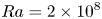 $Ra={2\times 10}^8$. This will be more evident in the following sections.
3.1.2. Thermal performance
The thermal performance is characterized by the average Nusselt number defined in (2.30). Different correlations have been proposed for  $Nu$ of tall enclosures following Gill's work (Ganguli et al. Reference Ganguli, Pandit and Joshi2009). Among them, Bejan (Reference Bejan1979) proposed the following correlation for tall enclosures:
 \begin{equation} Nu=C_B{\left[\frac{Ra}{Pr\,AR}\right]}^{0.25} \int_{-g_{e}}^{g_{e}}{\frac{{\left(1-g\right)}^6{\left(1+g\right)}^2(7-g^2)}{(1+g^2){(1+3g^2)}^{14/3}}\,{\rm d}g}, \end{equation}
where  $C_B$ and
  $g_e$ are functions of
  $({H}/{L})Ra^{1/7}_L$ (Bejan Reference Bejan1979). Here,
  $Ra_L=({L}/{H})^3/Ra={g\beta \Delta TL^3}/{\nu \alpha }$ is the Rayleigh number defined based on the width
  $L$, instead of the height
  $H$ as the characteristic length scale. While it is generally agreed that
  $Nu\sim Ra^{1/4}$, multiple studies have proposed slight modifications to this relation based on their observations. For example, another widely used correlation proposed by El Sherbiny et al. (Reference El Sherbiny, Raithby and Hollands1982) is
 \begin{equation} Nu=\max\left(Nu_1,Nu_2,Nu_3\right), \end{equation}
where  $Nu_1,Nu_2$, and
  $Nu_3$ are calculated from
 \begin{equation} \left.\begin{gathered}
Nu_1=0.0605Ra^{1/3}_L,\quad
Nu_2={\left[1+{\left[\frac{0.104Ra^{0.293}_L}{1+{\left(\dfrac{6310}{Ra_L}\right)}^{1.36}}\right]}^3\right]}^{1/3},\\
Nu_3=0.242{\left(\frac{Ra_L}{AR}\right)}^{0.272}.
\end{gathered}\right\}\end{equation}
\begin{equation} \left.\begin{gathered}
Nu_1=0.0605Ra^{1/3}_L,\quad
Nu_2={\left[1+{\left[\frac{0.104Ra^{0.293}_L}{1+{\left(\dfrac{6310}{Ra_L}\right)}^{1.36}}\right]}^3\right]}^{1/3},\\
Nu_3=0.242{\left(\frac{Ra_L}{AR}\right)}^{0.272}.
\end{gathered}\right\}\end{equation}
Figure 4 shows a comparison of  $Nu$ calculated by (2.31) (dotted lines), Bejan's equation (3.1) (dashed lines) and Elsherbiny's equation (3.2) (solid lines) along with the values from the present study (symbols). Bejan's correlation has been shown to over-predict the Nusselt number (Turan et al. Reference Turan, Poole and Chakraborty2012). Elsherbiny's correlation was proposed for
  $AR>5$, and it produces satisfactory results in that range. However, it also over-predicts the
  $Nu$ for smaller aspect ratio enclosures. Correlation (2.31) is based on the boundary-layer model discussed in § 2.3. The temperature solution (2.28) is based on an exponentially decreasing profile approaching the core temperature
  $T_0$, and therefore, the Nusselt number directly depends on the temperature difference of the wall and core,
  $\Delta T ={T}_H-{T }_0$, instead of the temperature difference of the enclosure walls,
  $\Delta T ={T}_H-{T}_C$, as it is usually defined for DHCs. The variation of
  ${T}_0$ with respect to
  $y$ is disposed of by taking the centreline (
 $y={H}/{2})$ or mean value
  ${T}_0={{\frac {1}{2}}}({T}_H+{T}_C)$. Therefore, we define
  $Ra$ based on
  $\Delta T ={T}_H-{{\frac {1}{2}}}({T}_H+{T}_C)$ noting that this temperature difference also appears in the Gill's so-called centrosymmetric property of differentially heated enclosures (Gill Reference Gill1966). In doing so, (2.31) gives a much better
  $Nu$ prediction (see figure 4 dotted curve), the present results (symbols) are in nearly perfect agreement with this correlation. At the end, this translates into a factor of
  $1/2$ in the
  $Ra$ and a factor of
  $(0.5)^{0.25}=0.8409$ in the calculation of
  $Nu$.
$Nu$.

Figure 4. Comparison of the average Nusselt number calculated by the direct numerical simulations (symbols) with the correlations given in the literature (Gill Reference Gill1966; Bejan Reference Bejan1979; El Sherbiny, Raithby & Hollands Reference El Sherbiny, Raithby and Hollands1982).
3.1.3. Time dependency and instability modes
As discussed in § 3.1.1, periodic time-dependent flow is observed for several cases. Time-dependent flow has been reported to exist only if  $Ra$ exceeds a critical value (
 $Ra_c$), which depends on
  $AR$ (Paolucci & Chenoweth Reference Paolucci and Chenoweth1989; Christon et al. Reference Christon, Gresho and Sutton2002; Xin & Le Quéré Reference Xin and Le Quéré2006). Specifically for
  $AR=2,4,6,8$, the critical Rayleigh number at which time-dependent flow emerges is
  $Ra_c=1.59\times {10}^8$,
  $1.03\times {10}^8$,
  $1.11\times {10}^8$ and
  $1.57\times {10}^8$ respectively, as reported by Xin & Le Quéré (Reference Xin and Le Quéré2006). Here, only
  $Ra=2\times {10}^8$ cases are above the critical value for all
  $AR$ values, and this is why only these cases exhibit time-dependent behaviour. This is further illustrated in figure 5 by plotting the time variations of
  $Nu/\overline {Nu}$ for
  $Ra=2\times {10}^8$ cases, where
  $\overline {Nu}$ denotes the time-averaged quantity of
  $Nu$. While consistent oscillatory behaviour is observed for these set-ups, the magnitude and frequency are different. The low
  $AR$ enclosures exhibit low-frequency oscillation compared with the high
  $AR$ enclosures due to the instability mechanism. We will discuss this effect later, along with the different instability modes. The magnitude of the oscillations shown in figure 5 increase as
  $Ra$ increases beyond
  $Ra_c$. When
  $AR=4$, the oscillation amplitude of
  $Ra=2\times 10^8$ is approximately twice
  $Ra_c$, while there is only
  $25\,\%$ increase compared with
  $Ra_c$ for
  $AR=2$. The higher amplitude fluctuations is observed for
  $AR=4$ enclosure.

Figure 5. Wall-average Nusselt number time dependence for  $Ra=2\times 10^8$.
The characteristic mode associated with the transition to time-dependent flow is of special interest and has also been reported by Xin & Le Quéré (Reference Xin and Le Quéré2006) wherein the modes are obtained from the linear stability analysis. From our direct numerical simulation results, extraction of the relevant modes is possible via modal decomposition techniques (Taira et al. Reference Taira, Brunton, Dawson, Rowley, Colonius, McKeon, Schmidt, Gordeyev, Theofilis and Ukeiley2017; Ramos et al. Reference Ramos, do Nascimento, Darze, Faccini and Giraldi2019; Vijayshankar et al. Reference Vijayshankar, Nabi, Chakrabarty, Grover and Benosman2020). The well-known dynamic mode decomposition (DMD) pioneered by Schmid (Reference Schmid2010) is used here to gain insight into the characteristic modes of the flow.
The flow data are represented by the matrix  $\boldsymbol{\mathsf{M}}=[{\boldsymbol{m}}(t_1)\ {\boldsymbol{m}}(t_2)\ \cdots {\boldsymbol{m}}(t_n)]$, where
  ${\boldsymbol{m}}(t_i)$ is the snapshot of the flow velocity and temperature at time
  $t_i$. DMD finds the best transition matrix
  ${\boldsymbol{\mathsf{A}}}$ such that
 \begin{equation} \boldsymbol{\mathsf{M}}_{2:n}=\boldsymbol{\mathsf{A}}\boldsymbol{\mathsf{M}}_{1:n-1}. \end{equation}
DMD modes and the associated frequencies are calculated using the singular value decomposition of the data matrix as follows Schmid (Reference Schmid2010)
 \begin{equation} \boldsymbol{\mathsf{M}}_{1:n-1}=\boldsymbol{\mathsf{U}}\,\boldsymbol{\Sigma}\,\boldsymbol{\mathsf{V}}^T. \end{equation}
 Defining  $\tilde {\boldsymbol{\mathsf{A}}}=\boldsymbol{\mathsf{U}}^T\,\boldsymbol{\mathsf{M}}_{2:n}\,(\boldsymbol{\mathsf{V}} \boldsymbol{\Sigma}^{-1})$, the eigenvalues
  $\mu _j$ and eigenvectors
  ${\boldsymbol{\phi} }_j$ of
  $\tilde {\boldsymbol{\mathsf{A}}}$ can be found and used to calculate
 \begin{equation} {\lambda }_j=\frac{1}{\Delta t}\log(\mu_j),\quad f_j=\frac{\mathrm{ang}\left({\lambda}_j\right)}{2{\rm \pi}}, \end{equation}
where  $\mathrm {ang}({\lambda }_j)$ is the phase angle of the complex eigenvalue
  ${\lambda }_j$, and
  $\Delta t=t_{i+1}-t_i$ is the time difference between data snapshots.
For buoyancy-driven flows, the coupled dynamics between the temperature and velocity field is critical, and therefore, the data vector is defined to preserve this coupling. Moreover, the decomposition in DMD must be accompanied by a choice of inner product and the corresponding norm or pseudo-energy function. The temperature and velocities are both used to form the observed data vector,  $\boldsymbol {m}={\{\gamma \theta,u,v\}}^\textrm {T}$. The scaling factor
  $\gamma =\langle uu+vv\rangle /\langle \theta \theta \rangle$ is adopted to make the dissimilar quantities of temperature and velocity consistent and energies comparable (Lumley & Poje Reference Lumley and Poje1997; Hasan & Sanghi Reference Hasan and Sanghi2007; Puragliesi & Leriche Reference Puragliesi and Leriche2012). The number of snapshots used to calculate modes depends on the period of oscillation of the
  $Nu$ for each case. At least 10 complete periods of the
  $Nu$ oscillation are included in the data matrix
  $\boldsymbol{\mathsf{M}}$. The time between snapshots is
  $\Delta t=0.5$ which corresponds to a sampling frequency of
  $2$. This is much larger than the highest anticipated the
  $Nu$ variation frequency of
  $0.1$. The number of snapshots used to calculate the modes was varied from 80 to 300. As long as at least one complete period of the
  $Nu$ oscillations was included, the results were similar within
  $1\,\%$ accuracy.
The dynamic modes associated with the time-dependent behaviour are shown in figure 6 for  $AR=1,2,4,6,8$. Two distinct modes can be identified: those observed only in the small
  $AR$ cases and the mode observed only in the large
  $AR$ cases. A similar observation has been made previously by Xin & Le Quéré (Reference Xin and Le Quéré2006) in which they found two types of modes: the first mode was observed in enclosures with the small aspect ratios
  $AR<3$ (henceforth referred to as
  ${\boldsymbol{\phi} }_s$) and the other was observed for the large
  $AR\ge 4$ (henceforth referred to as
  ${\boldsymbol{\phi} }_l$). They associated the first mode,
  ${\boldsymbol{\phi} }_s$ with angled internal waves encompassing the entire enclosure (similar to what is shown for
  $AR=1$ in figure 6). This mode is generated by the separation at the end of the vertical boundary layers where the flow impinges the top and bottom horizontal walls. However, there has not been a consensus about what physical mechanism causes instability. They described the second mode as a travelling wave mode confined to the boundary layer (similar to
  $AR=8$ in figure 6).

Figure 6. Time-dependent DMD modes for all aspect ratios and  $Ra=2\times 10^8$. Only
  $Ra=2\times 10^8$ exhibits time-dependent modes.
In this study, we also observed the two modes reported by the stability analysis of Xin & Le Quéré (Reference Xin and Le Quéré2006). However, it is  ${\boldsymbol{\phi} }_s$ and not
  ${\boldsymbol{\phi} }_l$ that is present in
  $AR=4$, different from the Xin and Le Quere's prediction. We note that the modes reported by them were for systems at the critical Rayleigh number,
  $Ra_c$, and our system is in the supercritical range (
 $Ra=2\times {10}^8>Ra_c=1.03\times {10}^8$). The streamlines for this case (figure 3) clearly show a separation region that is associated with
  ${\boldsymbol{\phi} }_s$. The frequency of this mode is
  $f=0.032$, the same as the frequency of the
  $Nu$ time history shown in figure 4. We are confident that
  ${\boldsymbol{\phi} }_s$ is the time-dependent mode for our system. The large
  $AR$ cases clearly show a travelling wave disturbance consisting of alternating positive and negative temperature fluctuation regions near the cavity walls. This mode travels in the clockwise direction and is similar to the unstable modes reported in the literature for the current configuration (Christon et al. Reference Christon, Gresho and Sutton2002; Xin & Le Quéré Reference Xin and Le Quéré2006). Like the small aspect ratio cases, the frequency associated with these modes matches the fluctuation frequency of
  $Nu$, with
  $f=0.43$ and
  $0.21$ for
  $AR=6$ and
  $8$ respectively.
3.2. DHC with CBCs
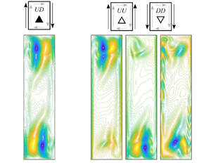
The configuration of the CBC can take four different conditions as shown and labelled in figure 7. The arrows on either side of the square represent the external flow direction, while the gravity always acts along the  $-y$ axis. Each configuration will be referred to by the first letter of external flow directions, e.g. UD corresponds to Up on the left and Down on the right (third configuration in figure 7). The effects of
  $AR$, and
  $Ra$ are studied for the same values as the previous section.

Figure 7. Configurations of the CBC and associated labels based on the direction of the external flow.
3.2.1. Effects on Nusselt number
The heat transfer of the system depends on the internal flow, characterized by  $Ra$, and the external flow, characterized by
  $Re$. The heat transfer at the wall can be treated as a lumped element system to explain the effects of the internal and external flows on the heat transfer and is written as
  $Q=\Delta T_w/R$. Here,
  $\Delta T_w$ is the temperature difference across the wall, and
  $R$ is the thermal resistance between the external and internal flow. Assuming zero thermal resistance from the wall (thin membrane), the total thermal resistance
  $R$ is a series of resistances due to the external boundary layer,
  $R_{ex}\sim k^{-1}Re^{-0.5}$, and internal boundary layer,
  $R_{in}\sim k^{-1}Ra^{-0.25}$ (Shu & Pop Reference Shu and Pop1999). This suggests that the ratio of thermal resistances
  $\varOmega =R_{in}/R_{ex}=Re^{0.5}Ra^{-0.25}$ can be employed to describe how the normalized Nusselt number changes as plotted in figure 8. The ratio
  $\varOmega$ can also be viewed as the ratio of the boundary-layer thickness of the external flow to the boundary-layer thickness of the internal flow. Therefore, a higher ratio represents a thinner external boundary layer relative to the internal flow. The symbols in figure 8 are based on what has been defined in figure 7. In figure 8 the isothermal boundary condition limit (dotted line) of the normalized Nusselt number is approached as the ratio
  $\varOmega$ increases for all configurations of CBC. We can see that, for lower
  $\varOmega$, the difference in
  $Nu$ between the different configurations is more significant. As
  $\varOmega$ increases, this difference between the configurations decreases as all configurations approach the isothermal limit. Specifically, for the case of
  $AR=4$, the isothermal boundary limit (- -) is not monotonically approached like the other cases.

Figure 8. Comparison of the normalized Nusselt number with respect to the ratio of the internal and external boundary-layers thickness ( $\varOmega ={Re}^{0.5}/Ra^{0.25}$) between the direct numerical simulation (DNS) results and boundary-layer model. See figure 7 (UD configuration
  $\blacktriangle$) (DU configuration
  $\blacktriangledown$) (DD configuration
  $\triangledown$) (UU configuration
  $\vartriangle$) (boundary-layer model UD configuration
  $\blacktriangle$, blue) (boundary-layer model DU configuration
  $\blacktriangledown$, blue) ((2.31) - -).
With respect to the influence of the configuration of the external flow, a clear trend is observed. The DU ( $\blacktriangledown$) configuration has the highest heat transfer among all CBC cases, while the UD (
 $\blacktriangle$) configuration has the lowest. The other configurations, UU and DD, show almost identical thermal characteristics in all cases. The heat transfer across the left enclosure wall is comprised of either parallel flow when the CBC is UD or UU, or counterflow when the CBC is DU or DD. This is true as long as the internal flow circulates in a clockwise fashion. A similar observation can be made for the right wall, parallel flow with the UD and DD CBC, and counterflow with DU and UU CBC. From the study of heat exchangers, it is known that the counterflow configurations always yield higher heat transfer rates. By comparison, it is not surprising that the DU CBC would yield the best heat transfer amongst the CBC cases since it has a counterflow configuration at both sidewalls.
The lower Nusselt number resulting from the boundary condition cases compared with the isothermal case is explained by the reduction of the average wall temperature due to the CBCs. The reduction in the average wall temperature effectively reduces the Rayleigh number of the system. The isothermal case can be viewed as a conjugate boundary case with infinite (or very large) Reynolds number flow, such that the temperature of the walls is unaffected. This may be very hard to achieve in practical applications or very costly. Therefore figure 8 is a comparison of the Nusselt number for various external flow speeds and the ideal infinite velocity (i.e. isothermal) case.
In addition to the computational results in figure 8, the analytical model of § 2.3 is applied to an enclosure with CBCs. The effects of the conjugate boundary condition on the Nusselt number are effectively captured in the multiplicative constant in (2.31). Due to the centrosymmetric restriction of the analytical model, only the UD and DU configurations are considered here, and the results are shown in figure 8 (blue symbols). Like in the isothermal boundary condition case, the boundary-layer model successfully predicts the thermal performance of most cases. However, we again see that the  $AR=4$ cases in the vicinity of
  ${Re}^{0.5}/Ra^{0.25}\approx 1$, deviate from the boundary-layer model.
Closer inspection of these cases (figure 9) shows the higher than expected  $Nu$ is due to a relatively higher mean free-stream velocity
  $\bar {v}$ and thinner boundary-layer thickness
  $\delta$. Unlike natural convection from a heated vertical plate, where the mean streamwise velocity (
 $\bar {v}$) is zero,
  $\bar {v}$ is non-zero for differentially heated vertical enclosures. Here, we define
  $\bar {v}$ as the maximum near-wall velocity along the height of the enclosure. The associated internal boundary-layer thickness can then be defined as
  $\delta =-(\Delta T/2)/(\textrm {d}\theta /{\textrm {d} x}|_w)$ (Zhou & Xia Reference Zhou and Xia2010; Zhou et al. Reference Zhou, Stevens, Sugiyama, Grossmann, Lohse and Xia2010; Scheel & Schumacher Reference Scheel and Schumacher2014; Ng et al. Reference Ng, Ooi, Lohse and Chung2015). We note that the boundary layers on the left and right walls are similar but develop in opposite directions, i.e. the left wall boundary layer develops in the
  $+y$ direction while the right wall boundary layer develops in the
  $-y$ direction. Additionally, the boundary layers are only similar if the flows are similar. This means that the right wall boundary layer with a CBC direction U (UU or UD configurations) is similar to a left wall boundary layer if the left wall CBC direction is D (DD or UD configurations).

Figure 9. Cases; (- -)  $AR=4$,
  $\varOmega =0.67$; (-)
  $AR=4$,
  $\varOmega =0.71$; (-.)
  $AR=6$,
  $\varOmega =0.71$; (:)
  $AR=2$,
  $\varOmega =0.71$. (a) Mean free-stream velocity, (b) boundary-layer thickness and (c) normalized Nusselt number. Here,
  $\langle {\cdot }\rangle$ denotes normalization of the argument by the corresponding isothermal case value.
A thin boundary layer results in higher heat transfer and therefore higher  $\bar {v}$ which ultimately leads to the impingement of the buoyant jet on the top and bottom walls on the left and right side of the enclosure, respectively. The impingement creates a separation region and secondary vortex near the ends of the side edges, which is the direct cause of the thinner boundary layer on the opposite side. The impingement and separation phenomena only occur in smaller aspect ratio cases (see figure 3). Similarly, the
  $AR=2$ enclosure exhibits the separation region at the end of the boundary layers as shown in figure 3(b). However, due to the wide aspect of the enclosure, the secondary vortex is relatively far from the opposite wall. Here, the separation and secondary vortex are positioned at
  $x/L\approx 0.25$ compared with
  $x/L\approx 0.6$ in the
  $AR=4$ enclosure. This allows for the flow to reattach in the
  $AR=2$ case, and the opposite wall boundary layer is not affected in the same way as in the
  $AR=4$ enclosure. We note that only in the cases with
  ${Re}^{0.5}/Ra^{0.25}\approx 1$ for
  $AR=4$, is the
  $\bar {v}$ high enough to create the separation region. In all other cases, the flow remains attached due to the reduction in the wall temperature, which leads to low
  $\bar {v}$.
While the increase in  $Nu$ is explained by the thinning of the boundary layer, the same cannot be said for the deviation of the boundary-layer model at these points (
 ${Re}^{0.5}/Ra^{0.25}\approx 1$). Unlike the isothermal case where the thermal capacity near the wall is reached before the end of the wall, CBC cases have a reduced wall temperature and therefore do not reach the full thermal capacity until the end of the wall. Indication of this is seen in 9(c) as the normalized
  $Nu$ is larger than unity for
  $y/H\ge 0.75$, which shows that in the isothermal case, the
  $Nu$ is defined primarily at the beginning of the wall and would not be significantly affected by secondary vortex and separation region at the end of the boundary layer. On the other hand, the CBC cases depend on the entire height of the wall to reach the thermal capacity, and the overall
  $Nu$ is affected by the end wall effects. Due to the linearization of the boundary-layer model, the end wall separation effect cannot be modelled and results in the less than perfect prediction of the heat transfer in the
  $AR=4$ and
  ${Re}^{0.5}/Ra^{0.25}\approx 1$ cases.
A power-law scaling of  $Nu\sim a{({H}/{L})}^b\,Ra^c$ is employed to predict the overall heat transfer in the CBC configuration. A similar relation has been tried for the problem of conjugate boundary layers of free convection on either side of a vertical wall (Anderson & Bejan Reference Anderson and Bejan1980; Treviño, Mendez & Higuera Reference Treviño, Mendez and Higuera1996). The difference is that, here, one side is forced convection and the other is natural convection, instead of both sides being natural convection. However, the principle is the same. In fact, when
  $Re^{0.5}Ra^{-0.25}=1$ in the DU configuration, the external and internal boundary-layer thicknesses are similar and the system is equivalent to the case examined in Anderson & Bejan (Reference Anderson and Bejan1980). Using the boundary-layer model of CBC configurations, the coefficients (
 $Nu\sim a{(H/L)}^bRa^c$) are identified as a function of
  $Re$ as
  $a=-1.1Re^{-0.24}+0.364$,
  $b=1.3Re^{-0.19}-1$,
  $c=-0.2Re^{-0.23}+0.25$. The correlation approaches the isothermal boundary case (2.31) in the high
  $Re$ limit. The predictions from the proposed relation are compared with the boundary-layer model results (colour) in figure 10 for different
  $Re$,
$Re$,  $Ra$ and selected aspect ratios where in the power-law relation agrees well with the theoretical boundary-layer model.

Figure 10. Comparison of the fitted  $Nu$ correlation (white contours) and the boundary-layer model (colour map).
3.2.2. Equivalent heat flux and Rayleigh number
In the previous section, we compared the thermal performance of the CBC cases at an equivalent external fluid temperature. Due to the CBC, the average wall temperature, and therefore the effective Rayleigh number was lower than the isothermal case. To reach a more pertinent comparison, in figure 11, the CBC cases and isothermal boundary condition DHC are compared at the same mean wall temperature, i.e. at the same effective Rayleigh number based on the temperature difference between two vertical walls ( $Ra_{eff}$). In figure 11(a,b) the ratio of CBC and isothermal cases heat fluxes are compared for two different
  $Ra$ for a typical external Reynolds number of
  $Re=5\times 10^3$. Note that the title denotes
  $Ra$ based on the external fluid temperature of the CBC; however, each point has an associated
  $Ra_{eff}$ at which an isothermal boundary condition case is compared. The heat flux of the CBC cases decreases with respect to the isothermal cases as
  $AR$ increases. It can also be observed that the difference between the different CBC configurations decreases as
  $AR$ increases. The difference between CBC configurations is also larger for the higher
  $Ra$ case, as is the CBC case heat fluxes compared with the isothermal case heat fluxes. In figure 11(c,d), the ratio of heat fluxes of the CBC and isothermal cases are shown for different external flow
  $Re$ and a fixed
  $Ra=10^8$. Similar trends are observed here; the CBC case's heat flux and the difference between CBC configurations decrease with increasing
  $AR$. We can see that as
  $\varOmega$, the ratio of internal to external thermal resistance defined in § 3.2.1, increases the differences between the CBC cases decreases. Looking at only the UD and DU configurations, which bound the data curves, it is clear that the difference between different CBC configurations is associated with the reduction in heat flux of the DU configurations. The UD, or parallel-flow configuration, cases always have approximately the same heat flux as the equivalent
  $Ra_{eff}$ isothermal case. It is interesting that for an equivalent
  $Ra_{eff}$, the heat flux
  $q$ from CBC configurations is higher than that of the isothermal boundary condition cases for most cases.

Figure 11. The ratio of the heat flux  $q$ of CBC cases to the heat flux
  $q_{iso}$ of an equivalent isothermal boundary case at an equivalent Rayleigh number
  $Ra_{eff}$ for different
  $AR$ values; (a,b) are for two
  $Ra$ cases with
  $Re=5\times 10^3$, and (c,d) are for two representative
  $Re$ cases with
  $Ra=10^8$.
While the average wall temperature difference is similar between the CBC and isothermal cases, the temperature profile along the walls is significantly different, as shown in figure 12. This leads to an increase in the heat flux compared with the isothermal case. Figure 12 shows the wall temperature profiles for select CBC cases normalized by the mean wall temperature, i.e. the isothermal boundary case with a uniform temperature profile. Two distinct shapes are observed corresponding to either a parallel or counterflow configuration at each wall. For example, the UU and UD configurations at the left wall (figure 12a,c) exhibit a parallel-flow configuration at the left wall and thus have a concave temperature profile. A similar profile is found along the right wall for the DD and UD configurations. The other observed temperature profile corresponds to the counterflow configuration, i.e. DD and DU configurations at the left wall (figure 12b,d) and the UU and DU configurations at the right wall (figure 12a,d). This profile monotonically increases along the wall's height with respect to the isothermal profile. Both types of temperature profiles increase the stratification of the core temperature in the mid-height region leading to higher heat transfer overall.

Figure 12. Wall temperature profiles for select CBC cases normalized by the mean wall temperature (wall temperature profile); (a–d) correspond to the left wall, and (e–h) correspond to the right wall. Solid line –  $AR=6$,
  $Re=10^4$,
  $Ra=2\times 10^8$; Dashed line is for
  $AR=6$,
 $Ra=2\times 10^8$ and different external Reynolds number case of
  $Re=10^3$; and dotted line is associated with smaller aspect ratio of
  $AR=4$, and
  $Re=10^4$,
  $Ra=2\times 10^8$.
3.2.3. Effect on flow and time-dependent modes
The effects of the conjugate boundaries extend beyond just the system's heat transfer. Differences in the streamlines and isotherms are hard to discern; instead, the dominant dynamic modes can be used to inspect the flow dynamics. The procedure discussed in § 3.1.3 is applied to the results obtained from the simulations of a cavity with CBCs. The external heat transfer in the CBC cases reduces the average wall temperature, thereby lowering the effective  $Ra$ (defined based on the wall temperatures). For the case with a large aspect ratio of
  $AR=8$ and
  $Re<{10}^4$, the reduction in the wall temperatures due to the external flow was sufficient to bring the system well below the critical Rayleigh number. Consequently, the system no longer exhibits the time-dependent characteristics observed in the isothermal case discussed in § 3.1.3. For
  $Re={10}^4$ cases, the effective
  $Ra$ remains above the critical value and the dynamic mode associated with time dependence is observed for all configurations of the CBC.
For the  $AR=6$ enclosure, the effective
  $Ra$ remains above
  $Ra_c$ for all configurations if
  $Re\ge 10^4$. Surprisingly, only the UD configuration exhibits the time-dependent mode associated with this aspect ratio (
 $\boldsymbol{\phi} _l$). The UD configuration, also referred to as the parallel-flow configuration, seems to be the only configuration to excite the instabilities leading to the time-dependent behaviour. While the
  $AR=6$ case does exhibit the time-dependent mode, its relative power is low, and no noticeable fluctuations can be found in the streamlines or temperature field. Previously, the critical Rayleigh number
  $Ra_c$ was discussed as the criterion for the onset time-dependent behaviour; however, it is clear that
  $Ra$ alone cannot predict the transition to time dependence in cases with external CBCs.
The  $AR=4$ enclosure similarly exhibits the time-dependent mode (
 $\boldsymbol{\phi} _s$) with the UD configuration for
  $Re=10^4$. The UU and DD configurations show time dependency, although they differ from those observed for the isothermal and UD boundary conditions. In figure 13, the time-dependent modes are shown for the case with
  $AR=4$,
  $Ra={2\times 10}^8$ and
  $Re={10}^4$ wherein the UU and DD cases introduce asymmetry to the flow and induce different time-dependent modes. The first dominant mode is similar to the previously observed time-dependent mode
  $\boldsymbol{\phi} _s$, but concentrated only at the ends of the enclosure. This can be seen in figure 13(a–c) where the latter 2 modes (b,c) split along the mid-height of the typical mode (a). These modes (b,c) have slightly different frequencies,
  $f_b=0.028$ and
  $f_c=0.026$, due to the difference in the mean free-stream velocity and the asymmetry of the corresponding external flow configurations.

Figure 13. DMD modes for  $AR=4$
  $Re=10^4$ and
  $Ra=2\times 10^8$. (a) The dominant time-dependent mode (
 $\phi _s$) for the UD configuration. (b–d) The 3 time-dependent modes present in the UU and DD configurations.
In addition, a new time-dependent mode emerges, different from what has been observed in low ( $\boldsymbol{\phi} _s$) and high (
 $\boldsymbol{\phi} _l$) aspect ratio cases. Figure 13(d) illustrates this new mode, which is a combination of the travelling wave mode in the boundary layer, and the mode associated with the impingement and separation at the end of the enclosures. This suggests that both modes can be present independently or together in enclosures with
  $AR=4$. A similar conclusion was made by Xin & Le Quéré (Reference Xin and Le Quéré2006) regarding such intermediate aspect ratios.
Surprisingly, in the case of  $AR=2$, the effective
  $Ra$ is always below the critical Rayleigh number, yet the time-dependent mode is still present for the UD configuration for the
  $Re=10^4$ and
  $Ra=2\times 10^8$ case due to conjugate thermal boundary condition. It is evident that the UD configuration has a destabilizing effect on the system. Although the effective
  $Ra$ is lower for the UD configuration than the other configurations, the fact that the UD cases always exhibit the time-dependent mode could translate into a more rapid transition to chaotic or turbulent flow at higher
  $Ra$. The DU configuration, on the other hand, can suppress the time-dependent modes even at supercritical Rayleigh numbers.
4. Conclusion
A numerical investigation and a reduced-order model of the flow and temperature of the natural convection inside a cavity with conjugate forced convection along the external side boundaries were presented. The effect of realistic thermal CBCs on the vertical sidewalls was investigated for different aspect ratios, internal Rayleigh number, external Reynolds number and external flow configurations. The average Nusselt number of sidewalls was explored to characterize the system's thermal performance. The isothermal boundary condition for each aspect ratio was compared with existing correlations and found to be in nearly perfect agreement with a minor modification of the temperature difference characteristic scale in the definition of the Rayleigh number. Modifying the definition of  $Ra$ with the appropriate characteristic temperature difference
  $\Delta T=T_H-0.5(T_H+T_C)$, instead of the usual enclosure wall temperature difference, significantly improved the
  $Nu$ predictions.
Furthermore, the flow dynamics was analysed by extracting the dynamic modes via DMD. A discrepancy was found for the time-dependent modes reported in the literature relative to the results presented here for  $AR=4$. It was observed that there are two time-dependent modes for the DHC systems, small aspect ratios are associated with the low-frequency mode
  ${\boldsymbol{\phi} }_s$, and the large aspect ratios are associated with the high-frequency travelling wave mode
  ${\boldsymbol{\phi} }_l$. Previously, mode
  ${\phi }_s$ was observed in
  $AR\le 3$ and mode
  ${\phi }_l$ in
  $AR\ge 4$, with multiple solutions existing between
  $3< AR<4$ at the critical Rayleigh number. Here, we showed that the mode
  ${\phi }_s$ is present in
  $AR\le 4$. We note that the
  $AR=4$ case with the low-frequency mode is at a supercritical Rayleigh number. However, the low-frequency mode
  ${\boldsymbol{\phi} }_s$ is associated with systems with detached flows at the end of the vertical boundary layers, which is the case for
  $AR=4$ even at subcritical Rayleigh numbers.
The influence of the CBC on the thermal performance is characterized by the two boundary layers formed on either side of the vertical walls. The heat flux through the wall is limited by the thermal resistance of each of the boundary layers. Increasing the thermal resistance ratio, or equivalently increasing  $Re$, enhances the heat transfer, and
  $Nu$ approaches the isothermal boundary condition limit. For specific cases, when the ratio of the thermal resistances is unity, both boundary layers are of equal size. Furthermore, it was found that the DU configuration (counterflow) at the vertical walls has the highest heat transfer while the lowest heat transfer is associated with UD configuration (parallel flow). This is consistent with the theory and observation made in heat exchangers in which counterflow configurations always yield the highest heat transfer. The boundary-layer model initially proposed by Gill (Reference Gill1966) was modified to include the CBC. While capable of accurately predicting most cases of
  $AR, Re, Ra$ and CBC configurations, it was shown that the model does not capture the response of cases affected by the separation region at the end walls. Besides these limited cases, the boundary-layer model provides a good estimation of
  $Nu$ based on the
  $Re,Ra$ and allows a relatively simple correlation for the heat transfer of these systems with or without CBC.
Comparing the CBC cases with the isothermal cases with equivalent Rayleigh numbers based on the vertical wall temperatures,  $Ra_{eff}$, it is found that, while the average wall temperature difference at the wall is the same for both CBC and isothermal cases, the non-uniform temperature profile of the CBC cases serves to increase the overall heat transfer. This is especially true for the DU configuration and lower
  $AR$ values.
The flow dynamics of the CBC configurations was also analysed using DMD. Although the time-dependent mode is present for  $AR=8$ and all CBC configurations, it is suppressed in smaller aspect ratios in all cases except the UD configuration. The
  $AR=4$ enclosure, however, has a modified time-dependent mode due to the asymmetry introduced by the UU and DD configurations. The modified mode is similar to the original mode
  ${\phi }_s$, but the top and bottom structures of the mode are at different frequencies. Surprisingly, for
  $AR=2$, the effective
  $Ra$ is always in the subcritical range, but the time-dependent mode is still present in the UD configuration. This leads us to believe that the wall temperature distribution of the UD configuration could result in an earlier transition to chaos/turbulence than would isothermal walls. In the future, the propagation of these effects at higher
  $Ra$ should be studied to verify the transition to chaotic flow.
The results show that the main difference between low and large aspect ratios is principally due to flow instability. Large aspect ratios develop a shear instability in the boundary layer, while small aspect ratios have a separation region caused by the wall jet impingement. The mismatch between  $Nu$ prediction of the boundary-layer model and numerical calculations for
  $AR=4$ is caused by this presence of the separation region as the nonlinear effect of the separation cannot be captured by the current boundary-layer model. This mismatch is almost not present in the isothermal case, where the thermal capacity of the system is reached before the separation region. The results align with previous observations about the flow transition in the cavities with
  $3< AR<4$ and suggest that this aspect ratio can be used to enhance the heat transfer without the need for large external flow velocity on the side edge, while the thermal performance of these optimal cases can further improve with the right choice of external flow directions, DU configuration in the current set-up. It is interesting to extend the study to three-dimensional cavity configurations to determine to what extent the observed trends persist.
Acknowledgements
The authors would also like to acknowledge the Florida State University Research Computing Center and the NAVY DSRC for the computational resources on which these simulations were carried out.
Funding
This material is based upon research supported by, or in part by, the U.S. Office of Naval Research (ONR) under award number ONR N00014-16-1-2956 Electric Ship Research and Development Consortium; any opinions, findings, and conclusions or recommendations are those of the authors and do not necessarily reflect the views of ONR. The paper's control number is DCN 43-9373-22.
Declaration of interests
The authors report no conflict of interest.
Appendix A
The following describes the boundary-layer model discussed in the main paper. The steps are similar to Gill (Reference Gill1966). However, for completeness, we present the derivation with the modified wall temperature condition. The equation for streamfunction, the conservation of momentum in vorticity form and the energy equation, all in dimensional form ( $*$) can be written as
 \begin{equation} \left.\begin{gathered} u^*={-}\frac{{\rm d}\psi^*}{{{\rm d} y}^*} \quad \text{and} \quad v^*=\frac{{\rm d}\psi^*}{{{\rm d} x}^*} \\ u^* \frac{{\rm d}\omega^*}{{{\rm d} x}^*}+v \frac{\partial \omega^*}{\partial y^* }=\nu\left(\frac{\partial^2 \omega^*}{\partial x^{*2}}+\frac{\partial^2 \omega^*}{\partial y^{*2}}\right)+g\beta \frac{\partial T^*}{\partial x} \\ u^*\frac{\partial T^*}{\partial x^*}+v^* \frac{\partial T^*}{\partial y^*}=\alpha \left(\frac{\partial ^2 T^*}{\partial x^{*2}}+\frac{\partial ^2 T^*}{\partial y^{*2}}\right), \end{gathered}\right\} \end{equation}
where the vorticity is
 \begin{equation} \omega^*=\frac{\partial ^2 \psi ^*}{\partial x^{*2}}+\frac{\partial ^2 \psi ^*}{\partial y^{*2}} . \end{equation}
The boundary conditions are given as
 \begin{equation} \left.\begin{gathered} \psi ^*=\frac{\partial \psi ^*}{\partial x^*}=0,\quad T^*=T_H \quad \text{at} \ x^*=0 ,\\ \psi ^*=\frac{\partial \psi ^*}{\partial x^*}=0,\quad T^*=T_C \quad \text{at} \ x^*=L ,\\ \psi ^*=\frac{\partial \psi ^*}{\partial y^*}=0,\quad \frac{\partial T^*}{\partial y^*}=0 \quad \text{at} \ y^*={\pm} \frac{1}{2}H. \end{gathered}\right\}\end{equation}
Defining the following non-dimensional variables:
 \begin{equation} \left.\begin{gathered} x=\frac{x^*}{\delta} ,\quad y=\frac{y^*}{H},\quad T=\frac{T^*-\frac{1}{2}(T_H+T_C )}{\Delta T},\quad \psi =\frac{\psi ^*\delta}{\alpha H} , \\ u=\frac{\delta}{\alpha} u^*,\quad v=\frac{\delta^2}{\alpha H} v^*,\quad \omega=\frac{\delta ^3}{\alpha H}\omega^*,\quad \delta =\frac{H}{Ra^{1/4}}, \end{gathered}\right\} \end{equation}
where  $\delta$ is the boundary-layer thickness, the boundary-layer equations can then be written in non-dimensional form as
 \begin{equation} \left.\begin{gathered} u={-}\psi_y, \quad v=\psi_x \\ u\,T_x+v\,T_y=T_{xx} \\ \frac{1}{Pr} (u\omega_x+v\omega_y )=\omega_{xx}+T_x \\ \omega=\psi_{xx}=v_x, \end{gathered}\right\} \end{equation}
and the boundary conditions at the wall are
 \begin{equation} \left.\begin{gathered} \psi =\psi _x=0,\quad T=T_w (y)\quad \text{at} \ x=0 \\ \psi =\psi _0 (y),\quad T=T_0 (y)\quad \text{at}\ x\to\infty \end{gathered}\right\}. \end{equation}
 As  $x\to \infty$, the solution must match the core solution. This approximation is only valid if the length of the cavity
  $L$ is much larger than the boundary layer
  $\delta$ or equivalently
 \begin{equation} \frac{L}{\delta} =\frac{L}{H} \left(\frac{Ra}{Pr}\right)^{1/4}\gg 1. \end{equation}
 The solutions of the flow and temperature fields near the vertical walls have been defined above by the boundary-layer problem. To deal with the nonlinearities of (A1), the Oseen linearization technique is used. The average value at each height  $y=\textrm {const}.$,
  $u_A$ and
  $T'_A$, are used as approximations in (A5). Integrating with respect to
  $x$ results in the following relations for
  $Pr\to \infty$:
 \begin{equation} \left.\begin{gathered} u_A\,T_x+T'_A\,v=T_{xx}, \\ 0=w_{xx}+T-T_0. \end{gathered}\right\} \end{equation}
 Equations (A8) make up a system of the fourth order in  $x$ such that the solution may be written as
 \begin{equation} w=\sum_{n=1}^4a_n(y) \exp({\lambda_n (y)x}), \end{equation}
where  $\lambda _n(y)$ are the roots of the quadratic equation
  $\lambda ^3 (\lambda +u_A )+T'_A=0$. This solution is valid for the whole boundary layer and the boundary conditions (A6) may then be applied to find
  $w$ and
  $\theta$
 $$\begin{gather} w=\frac{(T_w-T_0)}{(\lambda _2^2-\lambda _1^2 )} \left(-{\rm e}^{-\lambda _2 x}+{\rm e}^{-\lambda _1 x} \right) , \end{gather}$$
 $$\begin{gather}\theta=T-T_0=\frac{(T_w-T_0)}{(\lambda _2^2-\lambda _1^2 )} \left(\lambda _2^2 {\rm e}^{-\lambda _2 x}-\lambda _1^2 {\rm e}^{-\lambda _1 x} \right). \end{gather}$$
 To relate the average values of  $u_A$ and
  $T'_A$ to the core values
  $u_0$ and
  $T'_0$, we use the von-Kármán–Polhausen integral method and define
 $$\begin{gather} \psi _0 (y)=\int_0^\infty v\,{\rm d}x , \end{gather}$$
 $$\begin{gather}\frac{\partial}{\partial y} \int_0^\infty v\theta\,{{\rm d}x}+\psi _0T_0'={-}\left.\frac{\partial \theta}{\partial x}\right|_{x=0}. \end{gather}$$
Substituting (A10) and (A11) into (A12) and (A13) results in
 $$\begin{gather} \psi _0=\frac{T_w-T_0}{\lambda _1 \lambda _2 (\lambda _1+\lambda _2)}, \end{gather}$$
 $$\begin{gather}\frac{{\rm d}}{{\rm d} y} \left(\frac{(T_w-T_0 )^2}{(2(\lambda _1+\lambda _2 )^3)}\right)+\psi _0 T_0'=(T_w-T_0 )\frac{\lambda _1+\lambda _2-(\lambda _1 \lambda _2)}{\lambda _1+\lambda _2} . \end{gather}$$
 Moreover, since the solution should be dependent only on the invariants  $\tau =\lambda _1+\lambda _2$ and
  $\chi =\lambda _1 \lambda _2$, we can rewrite it as
 \begin{equation} \frac{{\rm d}}{{\rm d} y} \left(\frac{(T_w-T_0 )^2}{(2\tau ^3 )}\right)+\psi _0 T_0'=(T_w-T_0 )\left(\tau -\frac{\chi}{\tau}\right), \end{equation}
and with the use of (A14),
 \begin{align} \frac{4\tau (T_w-T_0 )(T_w'-T_0' )-6(T_w-T_0 )^2 \tau '}{4\tau ^4 }+\frac{(T_w-T_0 )}{\tau \chi} T_0'=(T_w-T_0 )\left(\tau -\frac{\chi}{\tau} \right). \end{align}
 Note  $u_A$ and
  $T_H$ are odd functions of
  $y$, therefore the four roots are
  $\lambda _1 (y)$,
  $\lambda _2 (y)$,
  $-\lambda _1(-y)$,
  $-\lambda _2(-y)$. Using these in the fourth-order polynomial for the roots, we can write the following relations:
 \begin{equation} \left.\begin{gathered} \tau ({-}y)-\tau (y)=u_A, \\ \chi (y)+\chi ({-}y)=\tau (y)\tau ({-}y), \\ \tau (y)\chi ({-}y)=\tau ({-}y)\chi (y), \\ \chi (y)\chi ({-}y)=T_A. \end{gathered}\right\} \end{equation}
 Next, the invariants can be recast in terms of odd and even functions  $q$, and
  $v$. The condition that
  $u_0,T_0,u_A,T_H$ are odd functions of
  $y$ can be used to simplify the equation. Here, the even function is defined by
 \begin{equation} h=\tau ({-}y)+\tau (y), \end{equation}
and the odd function by
 \begin{equation} p=u_A/h, \end{equation}
to express the solutions of  $\tau$ and
  $\chi$ as
 \begin{equation} \left.\begin{gathered} \tau =\tfrac{1}{2} h(1-p), \\ \chi =\tfrac{1}{8} h^2 (1-p^2 )(1-p), \\ \lambda _{1,2} =\tfrac{1}{4} h(1-p)[1\pm {\rm i}\sqrt{1+2p}]. \end{gathered}\right\} \end{equation}
 Equations (A21) and (A14) provide the solution for  $T_0$ and
  $\psi _0$. In particular, since
  $\psi _0$ is an even function of
  $y$, the odd part must be zero, and
  $T_0$ can be expressed as
 \begin{equation} T_0=\frac{1}{2} \left(T_w (y)-T_w ({-}y)\right)+\frac{q}{1+q^2} \left(T_w (y)+T_w ({-}y)\right). \end{equation}
Similarly, the solution for  $\psi _0$ is given as
 \begin{equation} \psi _0=\frac{8(T_w (y)+T_w ({-}y))}{h^3 (1-p^4)}. \end{equation}
 Finally, we can rewrite (A17) using the  $T_0$ expression as
 \begin{align} &[7-4p+3p^2 ](T_w+\bar{T}_w ) p'-\frac{3(T_w+\bar{T}_w )(1-p)(1+p^2 )}{h} h'- \frac{1}{8} h^4 (1-p)^4 (1+p^2 )^2 \nonumber\\ &\quad +\left(\frac{(2(1+p^2 )(3+p^2))}{(1-p)} \right) T_w' - \left(\frac{2(1+p^2 )(1-p)^3}{(1-p^2 )}\right) \bar{T}_w^{\prime}=0, \end{align}
where  $\bar {T}_w=T_w(-y)$ and
  $\bar {T}_w^{\prime }=T_w'(-y)$. This is the governing equation for the boundary layer on the left wall of the enclosure. The same equation can be written for the right side of the enclosure. However, due to the centrosymmetric property of the system., we can solve for the even and odd parts of (A24). The odd part being
 \begin{align} &-8(T_w+\bar{T}_w )pp'-\frac{6(T_w+\bar{T}_w )(1+p^2 )}{h} h'+ph^4 (1+p^2 )^3 \nonumber\\ &\quad +\frac{4(1+p^2 )(2+p+p^2 )}{(1-p)} T_w' - \frac{4(1+p^2 )(2-p+p^2 )}{(1+p)} T_w'=0 \end{align}
and the even part
 \begin{align} &(14+6p^2 )(T_w+\bar{T}_w ) p'+\frac{6p(T_w+\bar{T}_w)(1+p^2 )}{h} h'- \frac{1}{4} h^4 (1+p^2 )^2 (1+6p^2+p^4 ) \nonumber\\ &\quad +4(1+p^2 ) T_w'=0. \end{align}
 The two coupled differential equations involve  $p$,
$p$,  $h$,
$h$,  $T_w$ and their derivatives with respect to
  $y$ and are subject to the boundary conditions
 \begin{equation} \int_0^L \rho cv^*T^*-k \frac{{\rm d}T^*}{{{\rm d} y}^*} {{\rm d} x}^*=0\quad \text{at}\ y^*={\pm} \frac{H}{2} . \end{equation}
This is equivalent to imposing a zero heat flux condition at the top and bottom of the enclosure as proposed by Bejan (Reference Bejan1979). Re-writing in our non-dimensional variables
 \begin{equation} \frac{L}{\delta} \int_0^{L/\delta}vT\,{\rm d}x -\frac{L\delta}{H} \int_0^{L/\delta}\frac{{\rm d}T}{{\rm d} y} {{\rm d} x}=0 \quad \text{at}\ y={\pm} \frac{H}{2} ,\end{equation}
where  $\delta =HRa^{-1/4}$ is the boundary-layer thickness. The first term of (A28) is for the convective effects and the second the conduction effects. The differential equations along with the boundary conditions can be solved as long as the temperature distribution at the wall (
 $T_w$) is known.


