


1 Introduction
Mixed thermal convection is omnipresent in nature, from micoscales to atmospheric scales, and it is distinctly different from its constituent modes, namely those of forced and natural convection. In forced convection, the Nusselt number (
 $Nu$
) is correlated with the Prandtl (
$Nu$
) is correlated with the Prandtl (
 $Pr$
) and Reynolds numbers (
$Pr$
) and Reynolds numbers (
 $Re$
), while in natural convection the Nusselt number can be expressed as a function of the Prandtl and Rayleigh (
$Re$
), while in natural convection the Nusselt number can be expressed as a function of the Prandtl and Rayleigh (
 $Ra$
) numbers for different flow configurations. However, it was first observed by Lemlich & Hoke (Reference Lemlich and Hoke1956) in an experimental study that the local Nusselt number distribution in natural convection over a heated cylinder is similar to the one in forced convection over the cylinder if an effective Reynolds number is used for natural convection. The thin laminar boundary layer theory has led to the generalization of this concept. In one of the first theoretical studies, Acrivos (Reference Acrivos1966) showed the equivalence of the mixed convection to forced convection for two asymptotic values of Prandtl numbers for laminar boundary layer conditions. In particular, Acrivos (Reference Acrivos1966) showed that the following equivalence between different dimensionless groups would result in the same local Nusselt number:
$Ra$
) numbers for different flow configurations. However, it was first observed by Lemlich & Hoke (Reference Lemlich and Hoke1956) in an experimental study that the local Nusselt number distribution in natural convection over a heated cylinder is similar to the one in forced convection over the cylinder if an effective Reynolds number is used for natural convection. The thin laminar boundary layer theory has led to the generalization of this concept. In one of the first theoretical studies, Acrivos (Reference Acrivos1966) showed the equivalence of the mixed convection to forced convection for two asymptotic values of Prandtl numbers for laminar boundary layer conditions. In particular, Acrivos (Reference Acrivos1966) showed that the following equivalence between different dimensionless groups would result in the same local Nusselt number:
 $$\begin{eqnarray}\displaystyle & Gr_{x}=Re_{x}^{2}Pr^{1/3}\quad \text{as }Pr\rightarrow \infty , & \displaystyle\end{eqnarray}$$
 $$\begin{eqnarray}\displaystyle & Gr_{x}=Re_{x}^{2}\quad \text{as }Pr\rightarrow 0, & \displaystyle\end{eqnarray}$$
where
 $Gr=Ra/Pr$
is the Grashof number. These results were later extended by Churchill & Usagi (Reference Churchill and Usagi1972) to construct correlations for the intermediate-range Prandtl numbers by taking the power mean of the asymptotic limits.
$Gr=Ra/Pr$
is the Grashof number. These results were later extended by Churchill & Usagi (Reference Churchill and Usagi1972) to construct correlations for the intermediate-range Prandtl numbers by taking the power mean of the asymptotic limits.
As noted recently by Churchill (Reference Churchill2014), the concept of equivalence has a great potential in that it provides a new structure for assembling data on thermal transport and a new means for predictive heat transfer. In that study, an equivalence expression
 $Gr_{x}=A\{Pr\}Re_{x}^{2}$
was formulated by seeking the coefficient of proportionality
$Gr_{x}=A\{Pr\}Re_{x}^{2}$
was formulated by seeking the coefficient of proportionality
 $A\{Pr\}$
between the Grashof number and the square of the Reynolds number. Churchill’s work revealed a surprising generality in predicting the Nusselt number for natural convection from forced convection or vice versa once the algebraic relationship
$A\{Pr\}$
between the Grashof number and the square of the Reynolds number. Churchill’s work revealed a surprising generality in predicting the Nusselt number for natural convection from forced convection or vice versa once the algebraic relationship
 $A\{Pr\}$
is discovered. Specifically,
$A\{Pr\}$
is discovered. Specifically,
 $A\{Pr\}$
varies smoothly for surfaces with uniform temperature to surfaces with uniform heat flux, and it holds true for a wide variety of geometries.
$A\{Pr\}$
varies smoothly for surfaces with uniform temperature to surfaces with uniform heat flux, and it holds true for a wide variety of geometries.
For mixed-convection flows the Nusselt number is a function of Reynolds number, Grashof number and the angle
 $\unicode[STIX]{x1D703}$
between the forced- and natural-convection directions (see figure 2
a). The majority of the studies so far have investigated the cases of aiding convection (
$\unicode[STIX]{x1D703}$
between the forced- and natural-convection directions (see figure 2
a). The majority of the studies so far have investigated the cases of aiding convection (
 $\unicode[STIX]{x1D703}=0^{\circ }$
) and opposing convection (
$\unicode[STIX]{x1D703}=0^{\circ }$
) and opposing convection (
 $\unicode[STIX]{x1D703}=180^{\circ }$
); see for example Acrivos (Reference Acrivos1966), Sparrow & Lee (Reference Sparrow and Lee1976), Churchill (Reference Churchill1977), Patnaik, Narayana & Seetharamu (Reference Patnaik, Narayana and Seetharamu1999), Sharma & Eswaran (Reference Sharma and Eswaran2004), Hu & Koochesfahani (Reference Hu and Koochesfahani2011). Most commonly, mixed-convection correlations are constructed by combining existing pure forced (
$\unicode[STIX]{x1D703}=180^{\circ }$
); see for example Acrivos (Reference Acrivos1966), Sparrow & Lee (Reference Sparrow and Lee1976), Churchill (Reference Churchill1977), Patnaik, Narayana & Seetharamu (Reference Patnaik, Narayana and Seetharamu1999), Sharma & Eswaran (Reference Sharma and Eswaran2004), Hu & Koochesfahani (Reference Hu and Koochesfahani2011). Most commonly, mixed-convection correlations are constructed by combining existing pure forced (
 $Nu_{F}$
) and natural (
$Nu_{F}$
) and natural (
 $Nu_{N}$
) convection correlations in the form of the power mean, i.e.
$Nu_{N}$
) convection correlations in the form of the power mean, i.e.
 $$\begin{eqnarray}Nu^{n}=Nu_{F}^{n}\pm Nu_{N}^{n},\end{eqnarray}$$
where the plus sign applies for the aiding flow and minus sign applies for opposing flow, and the exponent
 $n$
is obtained as the best fit to the data. In the above expression,
$n$
is obtained as the best fit to the data. In the above expression,
 $Nu_{N}$
is commonly replaced by an equivalent forced-convection Nusselt number (see Churchill Reference Churchill1977 and references therein).
$Nu_{N}$
is commonly replaced by an equivalent forced-convection Nusselt number (see Churchill Reference Churchill1977 and references therein).
The effect of continuous variation of
 $\unicode[STIX]{x1D703}$
on the Nusselt number is relatively underexplored. Oosthuizen & Madan (Reference Oosthuizen and Madan1971) investigated the effect of flow directionality for
$\unicode[STIX]{x1D703}$
on the Nusselt number is relatively underexplored. Oosthuizen & Madan (Reference Oosthuizen and Madan1971) investigated the effect of flow directionality for
 $\unicode[STIX]{x1D703}=0^{\circ },90^{\circ },135^{\circ }$
and
$\unicode[STIX]{x1D703}=0^{\circ },90^{\circ },135^{\circ }$
and
 $180^{\circ }$
. For a fixed
$180^{\circ }$
. For a fixed
 $\unicode[STIX]{x1D703}$
, they proposed a correlation of the form
$\unicode[STIX]{x1D703}$
, they proposed a correlation of the form
 $Nu/Nu_{f}=f(Gr/Re^{2})$
, where
$Nu/Nu_{f}=f(Gr/Re^{2})$
, where
 $Nu_{f}$
is the corresponding Nusselt number at the same forced-convection flow. However, no universal correlation in the form
$Nu_{f}$
is the corresponding Nusselt number at the same forced-convection flow. However, no universal correlation in the form
 $Nu=f(Re,Gr,\unicode[STIX]{x1D703})$
was suggested. For other values of
$Nu=f(Re,Gr,\unicode[STIX]{x1D703})$
was suggested. For other values of
 $0^{\circ }<\unicode[STIX]{x1D703}<180^{\circ }$
, Hatton, James & Swire (Reference Hatton, James and Swire1970) introduced an effective Reynolds number by vectorially adding the Reynolds numbers of the forced convection and the equivalent natural convection (see (3.8)). The effective Reynolds number was then used in the forced-convection correlation to predict the Nusselt number around a heated cylinder. Therefore, this yields a correlation for the Nusselt number as a function of
$0^{\circ }<\unicode[STIX]{x1D703}<180^{\circ }$
, Hatton, James & Swire (Reference Hatton, James and Swire1970) introduced an effective Reynolds number by vectorially adding the Reynolds numbers of the forced convection and the equivalent natural convection (see (3.8)). The effective Reynolds number was then used in the forced-convection correlation to predict the Nusselt number around a heated cylinder. Therefore, this yields a correlation for the Nusselt number as a function of
 $Nu=f(Re,Gr,\unicode[STIX]{x1D703})$
. However, for opposing convection, the flow dynamics is distinctly different from its corresponding ‘equivalent’ forced convection. As Hatton et al. (Reference Hatton, James and Swire1970) and several other investigators (Badr Reference Badr1984; Sharma & Eswaran Reference Sharma and Eswaran2004) have indicated, this approach yields unsatisfactory results for opposing convection i.e.
$Nu=f(Re,Gr,\unicode[STIX]{x1D703})$
. However, for opposing convection, the flow dynamics is distinctly different from its corresponding ‘equivalent’ forced convection. As Hatton et al. (Reference Hatton, James and Swire1970) and several other investigators (Badr Reference Badr1984; Sharma & Eswaran Reference Sharma and Eswaran2004) have indicated, this approach yields unsatisfactory results for opposing convection i.e.
 $90^{\circ }<\unicode[STIX]{x1D703}<180^{\circ }$
. These observations suggest an incomplete similarity of the Nusselt number with respect to the angle
$90^{\circ }<\unicode[STIX]{x1D703}<180^{\circ }$
. These observations suggest an incomplete similarity of the Nusselt number with respect to the angle
 $\unicode[STIX]{x1D703}$
.
$\unicode[STIX]{x1D703}$
.

Figure 1. Nusselt number versus effective Reynolds number for mixed convection around a cylinder obtained from the experiments of Hatton et al. (Reference Hatton, James and Swire1970) (blue symbols) and our direct numerical simulations (DNS) (red symbols). The black curve suggested by Hatton et al. (Reference Hatton, James and Swire1970), corresponds to a correlation obtained from the ‘equivalence’ concept using experimental data from forced and natural convection. The disparity observed is due to parametric space compression, which is here represented by the effective Reynolds number, i.e.
 $Re_{eff}$
(see the main text for more explanation). In the present study, the experimental correlation is employed as a low-fidelity approximation for the mixed convection, while the high-fidelity approximation is obtained from DNS.
$Re_{eff}$
(see the main text for more explanation). In the present study, the experimental correlation is employed as a low-fidelity approximation for the mixed convection, while the high-fidelity approximation is obtained from DNS.
The combined error induced by using the concept of equivalence between the two flows, and the vectorial addition of the forced-convection and natural-convection Reynolds number can be significant. In figure 1, the Nusselt number versus the effective Reynolds number
 $Re_{eff}$
obtained from the experimental measurements (blue symbols) by Hatton et al. (Reference Hatton, James and Swire1970), the experimental correlation (black curve), and the direct numerical simulation (DNS) (red symbols) are shown. Note that the experimental and numerical samples are not necessarily at the same
$Re_{eff}$
obtained from the experimental measurements (blue symbols) by Hatton et al. (Reference Hatton, James and Swire1970), the experimental correlation (black curve), and the direct numerical simulation (DNS) (red symbols) are shown. Note that the experimental and numerical samples are not necessarily at the same
 $Re$
,
$Re$
,
 $Gr$
and
$Gr$
and
 $\unicode[STIX]{x1D703}$
. Since the specific values of
$\unicode[STIX]{x1D703}$
. Since the specific values of
 $Re$
,
$Re$
,
 $Gr$
and
$Gr$
and
 $\unicode[STIX]{x1D703}$
are not specified in the experimental study, a one-to-one correspondence between the DNS and experimental measurements cannot be established. It is clear that the experimental correlation exhibits variable degree of fidelity as a function of
$\unicode[STIX]{x1D703}$
are not specified in the experimental study, a one-to-one correspondence between the DNS and experimental measurements cannot be established. It is clear that the experimental correlation exhibits variable degree of fidelity as a function of
 $Re_{eff}$
. It appears that for larger values of
$Re_{eff}$
. It appears that for larger values of
 $Re_{eff}$
, the correlation is more accurate than for the lower
$Re_{eff}$
, the correlation is more accurate than for the lower
 $Re_{eff}$
.
$Re_{eff}$
.
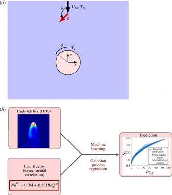
Figure 2. (a) Schematic of mixed convection of flow over a cylinder. The average Nusselt number of mixed convection for flow over a cylinder is expressed as
 $Nu=f(Re,Ri,\unicode[STIX]{x1D703})$
. (b) Multi-fidelity modelling framework.
$Nu=f(Re,Ri,\unicode[STIX]{x1D703})$
. (b) Multi-fidelity modelling framework.
However, despite the discrepancy between the correlation and the experimental/DNS results, the equivalence theory (black curve) still captures the major trend of variation of the average Nusselt number versus the effective Reynolds number. In other words, the corresponding correlation provides an acceptable variation of the
 $Nu$
versus
$Nu$
versus
 $Re_{eff}$
albeit somewhat erroneous. We will consider this correlation as a model for the Nusselt number that contains low-fidelity information. On the other hand, the DNS response serves as an accurate prediction and therefore it contains high-fidelity information. It is therefore desirable to exploit the low-fidelity response of the system, particularly since it is cheap to sample it. The objective of the current study is to blend the low-fidelity experimental response with a relatively small number of high-fidelity DNS runs in an information-fusion framework, and to construct a stochastic response surface that will serve as a significant improvement to the empirical correlation used so far in mixed convection.
$Re_{eff}$
albeit somewhat erroneous. We will consider this correlation as a model for the Nusselt number that contains low-fidelity information. On the other hand, the DNS response serves as an accurate prediction and therefore it contains high-fidelity information. It is therefore desirable to exploit the low-fidelity response of the system, particularly since it is cheap to sample it. The objective of the current study is to blend the low-fidelity experimental response with a relatively small number of high-fidelity DNS runs in an information-fusion framework, and to construct a stochastic response surface that will serve as a significant improvement to the empirical correlation used so far in mixed convection.
Combining low-fidelity models with high-fidelity models is not a trivial task, and it is only possible if modelling and parametric uncertainties at every level of fidelity are taken explicitly into account. In the present work, we adopt a non-parametric Bayesian regression framework that is capable of blending information from sources of different fidelity, and provides a predictive posterior distribution from which we can infer quantities of interest with quantified uncertainty. Our work is inspired by the pioneering work of Kennedy & O’Hagan (Reference Kennedy and O’Hagan2000) and relies on Gaussian process (GP) regression at the high-fidelity level (DNS) and the low-fidelity level (experimental correlation). This supervised learning approach is based on parametrizing pre-specified autocorrelation kernels via the proper hyper-parameters, which are subsequently computed on-the-fly from observed data, along with the bias or modelling error at every level of fidelity. The technical details will be shown later in § 3.3, but it suffices here to say that a key component of this methodology is the exploration of cross-correlations between the high-fidelity and low-fidelity quantities. Moreover, leveraging the probabilistic structure of the GP predictive posterior distribution, one may design intelligent sampling strategies for further data acquisition. In particular, by exploring the mean and variance values, we can assess the improvement of the predictability of the response surface by selecting new ‘sweet spots’ where new experiments or DNS can be used as new samples of high-fidelity information. This framework, therefore, provides a new paradigm in predicting heat transfer, one that employs heavily existing experimental correlations and enhances greatly their utility by combining them with high-fidelity information from DNS or from detailed experimental measurements using e.g. PIV (particle image velocimetry) or DPIV (digital particle image velocimetry) and DPIT (digital particle image thermometry) (Ronald Reference Ronald1991; Pereira et al. Reference Pereira, Gharib, Dabiri and Modarress2000; Eckstein & Vlachos Reference Eckstein and Vlachos2009). This field information is also very useful in elucidating the physics of the flow and especially in cases where anomalous transport or interesting dynamics may be revealed by the data or the multi-fidelity surrogate model.
The rest of the paper is organized as follows: in § 2 we introduce the statement of the problem that involves mixed convection around a heated cylinder. In § 3 we present an overview of the multi-fidelity framework and in § 4 cross-validation results. In § 5 we present the multi-fidelity results and we conclude in § 6 with a short summary.
2 Problem statement
The schematic of the problem is shown in figure 2(a). The origin of the coordinate system is at the centre of the cylinder,
 $\boldsymbol{e}_{x}$
and
$\boldsymbol{e}_{x}$
and
 $\boldsymbol{e}_{y}$
denote the unit vector in the
$\boldsymbol{e}_{y}$
denote the unit vector in the
 $x$
and
$x$
and
 $y$
directions respectively and
$y$
directions respectively and
 $\boldsymbol{e}_{g}$
is the unit vector along the direction of gravity. The angle between
$\boldsymbol{e}_{g}$
is the unit vector along the direction of gravity. The angle between
 $U_{\infty }$
and gravity
$U_{\infty }$
and gravity
 $\boldsymbol{g}=g\boldsymbol{e}_{g}$
is denoted by
$\boldsymbol{g}=g\boldsymbol{e}_{g}$
is denoted by
 $\unicode[STIX]{x1D703}$
. As such,
$\unicode[STIX]{x1D703}$
. As such,
 $\unicode[STIX]{x1D703}=0^{\circ }$
represents aiding convection,
$\unicode[STIX]{x1D703}=0^{\circ }$
represents aiding convection,
 $\unicode[STIX]{x1D703}=180^{\circ }$
opposing convection and
$\unicode[STIX]{x1D703}=180^{\circ }$
opposing convection and
 $\unicode[STIX]{x1D703}=90^{\circ }$
cross-flow convection. The surface temperature of the cylinder is denoted by
$\unicode[STIX]{x1D703}=90^{\circ }$
cross-flow convection. The surface temperature of the cylinder is denoted by
 $T_{s}$
and the far field temperature by
$T_{s}$
and the far field temperature by
 $T_{\infty }$
.
$T_{\infty }$
.
The problem of mixed-convection flow over a cylinder can be characterized by three non-dimensional parameters of Reynolds number, namely
 $Re=U_{\infty }D/\unicode[STIX]{x1D708}$
, Richardson number
$Re=U_{\infty }D/\unicode[STIX]{x1D708}$
, Richardson number
 $Ri=Gr/Re^{2}$
and
$Ri=Gr/Re^{2}$
and
 $\unicode[STIX]{x1D703}$
, where
$\unicode[STIX]{x1D703}$
, where
 $Gr=g\unicode[STIX]{x1D6FD}(T_{s}-T_{\infty })D^{3}/\unicode[STIX]{x1D708}^{2}$
is the Grashof number and
$Gr=g\unicode[STIX]{x1D6FD}(T_{s}-T_{\infty })D^{3}/\unicode[STIX]{x1D708}^{2}$
is the Grashof number and
 $D$
is the diameter of the cylinder,
$D$
is the diameter of the cylinder,
 $\unicode[STIX]{x1D708}$
is the kinematic viscosity of the fluid and
$\unicode[STIX]{x1D708}$
is the kinematic viscosity of the fluid and
 $\unicode[STIX]{x1D6FD}$
is the thermal expansion rate. Therefore, the average Nusselt number can be written as a function of these three parameters:
$\unicode[STIX]{x1D6FD}$
is the thermal expansion rate. Therefore, the average Nusselt number can be written as a function of these three parameters:
 $$\begin{eqnarray}Nu=f(Re,Ri,\unicode[STIX]{x1D703}).\end{eqnarray}$$
The objective of this study is to seek the above functional map
 $f$
. We do so by combining a relatively small number of high-fidelity DNS with a large number of samples drawn from existing experimental correlations. The three parameters constitute a three-dimensional parametric space denoted by
$f$
. We do so by combining a relatively small number of high-fidelity DNS with a large number of samples drawn from existing experimental correlations. The three parameters constitute a three-dimensional parametric space denoted by
 $\boldsymbol{x}=\{Re,Ri,\unicode[STIX]{x1D703}\}$
. We consider the following ranges for each dimension:
$\boldsymbol{x}=\{Re,Ri,\unicode[STIX]{x1D703}\}$
. We consider the following ranges for each dimension:
 $$\begin{eqnarray}0\leqslant Re\leqslant 40,\quad 0\leqslant Ri\leqslant 1\quad \text{and}\quad 0^{\circ }\leqslant \unicode[STIX]{x1D703}\leqslant 180^{\circ }.\end{eqnarray}$$
We note that
 $Ri=0$
corresponds to pure forced convection and
$Ri=0$
corresponds to pure forced convection and
 $Re=0$
corresponds to pure natural convection. The angle
$Re=0$
corresponds to pure natural convection. The angle
 $\unicode[STIX]{x1D703}$
varies continuously from aiding flow (
$\unicode[STIX]{x1D703}$
varies continuously from aiding flow (
 $\unicode[STIX]{x1D703}=0^{\circ }$
) to opposing flow (
$\unicode[STIX]{x1D703}=0^{\circ }$
) to opposing flow (
 $\unicode[STIX]{x1D703}=180^{\circ }$
). We choose the fluid to be air with
$\unicode[STIX]{x1D703}=180^{\circ }$
). We choose the fluid to be air with
 $Pr=0.7$
in our entire study.
$Pr=0.7$
in our entire study.
3 Multi-fidelity framework
In this section we describe both the high- and the low-fidelity models, and present how the predictions from these two models are combined to yield a multi-fidelity stochastic response surface for the average Nusselt number (see figure 2 b).
3.1 High-fidelity model
As a high-fidelity approximation, we consider the incompressible flow, along with the Boussinesq approximation, to model the mixed convection. These equations in non-dimensional form are given by:
 $$\begin{eqnarray}\displaystyle & \displaystyle \unicode[STIX]{x1D735}\boldsymbol{\cdot }\boldsymbol{u}=0, & \displaystyle\end{eqnarray}$$
 $$\begin{eqnarray}\displaystyle & \displaystyle \frac{\unicode[STIX]{x2202}\boldsymbol{u}}{\unicode[STIX]{x2202}t}+(\boldsymbol{u}\boldsymbol{\cdot }\unicode[STIX]{x1D735})\boldsymbol{u}=-\unicode[STIX]{x1D735}p+{\displaystyle \frac{1}{Re}}\unicode[STIX]{x1D6FB}^{2}\boldsymbol{u}+RiT\boldsymbol{e}_{\boldsymbol{ g}}, & \displaystyle\end{eqnarray}$$
 $$\begin{eqnarray}\displaystyle & \displaystyle \frac{\unicode[STIX]{x2202}T}{\unicode[STIX]{x2202}t}+(\boldsymbol{u}\boldsymbol{\cdot }\unicode[STIX]{x1D735})T={\displaystyle \frac{1}{RePr}}\unicode[STIX]{x1D6FB}^{2}T. & \displaystyle\end{eqnarray}$$
We solve the above equations at a relatively low Reynolds number and in a two-dimensional domain whose schematic is shown in figure 2(a). The forced convection is enforced at the top boundary condition via
 $\boldsymbol{u}=-U_{\infty }\boldsymbol{e}_{y}$
and
$\boldsymbol{u}=-U_{\infty }\boldsymbol{e}_{y}$
and
 $T_{\infty }=0$
, and on all other side boundaries convective outflow boundary condition is used. On the cylinder surface, the no-slip boundary condition and the isothermal boundary condition
$T_{\infty }=0$
, and on all other side boundaries convective outflow boundary condition is used. On the cylinder surface, the no-slip boundary condition and the isothermal boundary condition
 $T_{s}=1$
are used.
$T_{s}=1$
are used.
We perform DNS using the spectral/hp element method (see reference Karniadakis & Sherwin (Reference Karniadakis and Sherwin2005) for more details of the spectral/hp element method and see references Babaee, Acharya & Wan (Reference Babaee, Acharya and Wan2013a
), Babaee, Wan & Acharya (Reference Babaee, Wan and Acharya2013b
) for validation of the code for heat transfer applications). We use a quadrilateral discretization with nearly 15 000 elements and spectral polynomial order of
 $P=4$
. The computational grid is shown in figure 3(a), and a close-up view of the mesh near the cylinder is shown in figure 3(b).
$P=4$
. The computational grid is shown in figure 3(a), and a close-up view of the mesh near the cylinder is shown in figure 3(b).
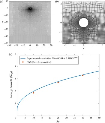
Figure 3. (a) Quadrilateral mesh for the DNS with nearly 15 000 elements and spectral polynomial
 $P=4$
; (b) close-up view of the mesh near the cylinder; (c) validation of DNS for forced convection around a heated cylinder. Comparison of the experimental correlation with DNS. The same correlation (3.4) is used for estimating the Nusselt number for mixed convection by replacing
$P=4$
; (b) close-up view of the mesh near the cylinder; (c) validation of DNS for forced convection around a heated cylinder. Comparison of the experimental correlation with DNS. The same correlation (3.4) is used for estimating the Nusselt number for mixed convection by replacing
 $Re$
with an effective Reynolds number
$Re$
with an effective Reynolds number
 $Re_{eff}$
from (3.8).
$Re_{eff}$
from (3.8).
We have validated the high-fidelity approximation for the case of pure forced convection. For the time-dependent cases we compute the time-averaged Nusselt number. In figure 3(c) the average Nusselt number obtained from DNS is compared against the experimental correlation that is presented later in (3.4). A good agreement is observed.
3.2 Low-fidelity model
The low-fidelity approximations are obtained based on the vectorial addition approach, first introduced by Hatton et al. (Reference Hatton, James and Swire1970). This approach is based on the concept of equivalence between natural-convection and forced-convection flows. In this approach, for a pure natural-convection flow at Rayleigh number
 $Ra$
, an equivalent Reynolds number
$Ra$
, an equivalent Reynolds number
 $Re_{n}$
is found such that the corresponding pure forced-convection flow at
$Re_{n}$
is found such that the corresponding pure forced-convection flow at
 $Re_{n}$
would generate the same Nusselt number as the pure natural-convection flow. This can be obtained by equating the correlations of forced and natural-convection flows given by:
$Re_{n}$
would generate the same Nusselt number as the pure natural-convection flow. This can be obtained by equating the correlations of forced and natural-convection flows given by:
 $$\begin{eqnarray}\displaystyle & Nu_{f}=0.384+0.581Re_{f}^{0.439},\text{ forced convection,} & \displaystyle\end{eqnarray}$$
 $$\begin{eqnarray}\displaystyle & Nu_{n}=0.384+0.59Ra^{0.184},\text{ natural convection,} & \displaystyle\end{eqnarray}$$
to obtain an equivalent Reynolds number:
 $$\begin{eqnarray}Re_{n}=1.03Ra^{0.418}.\end{eqnarray}$$
For a mixed-convection flow, an effective Reynolds number is calculated based on the vector addition of the forced convection and natural convection (Hatton et al. Reference Hatton, James and Swire1970):
 $$\begin{eqnarray}Re_{eff}=|Re_{f}\boldsymbol{e}_{y}+Re_{n}\boldsymbol{e}_{g}|,\end{eqnarray}$$
from which we obtain the effective Reynolds number (for air):
 $$\begin{eqnarray}Re_{eff}^{2}=Re_{f}^{2}\left[1+2.06\left(\frac{Ra^{0.418}}{Re_{f}}\right)\cos \unicode[STIX]{x1D703}+1.06\left(\frac{Ra^{0.836}}{Re_{f}^{2}}\right)\right].\end{eqnarray}$$
The effective Reynolds number
 $Re_{eff}$
is then used to compute the average Nusselt number from (3.4). Therefore, the low-fidelity model is given by:
$Re_{eff}$
is then used to compute the average Nusselt number from (3.4). Therefore, the low-fidelity model is given by:
 $$\begin{eqnarray}Nu^{LF}=0.384+0.581Re_{eff}^{0.439}.\end{eqnarray}$$
The above approach approximates the average Nusselt number with a variable degree of accuracy. To investigate this more closely, in figure 4 three cases of aiding flow (
 $\unicode[STIX]{x1D703}=0^{\circ }$
), cross-flow (
$\unicode[STIX]{x1D703}=0^{\circ }$
), cross-flow (
 $\unicode[STIX]{x1D703}=90^{\circ }$
) and opposing flow (
$\unicode[STIX]{x1D703}=90^{\circ }$
) and opposing flow (
 $\unicode[STIX]{x1D703}=180^{\circ }$
) at
$\unicode[STIX]{x1D703}=180^{\circ }$
) at
 $Re=40$
and
$Re=40$
and
 $Ri=1$
are shown. The first column shows the local and average Nusselt number, and the second and third columns show the equivalent forced convection at
$Ri=1$
are shown. The first column shows the local and average Nusselt number, and the second and third columns show the equivalent forced convection at
 $Re_{eff}$
and the mixed convection at the corresponding angle
$Re_{eff}$
and the mixed convection at the corresponding angle
 $\unicode[STIX]{x1D703}$
.
$\unicode[STIX]{x1D703}$
.

Figure 4. (a,d,g) The local (solid lines: DNS) and the average (dashed lines: DNS) Nusselt number. (b,e,h) Mixed convection at
 $Re=40$
and
$Re=40$
and
 $Ri=1$
. The circles correspond to experimental correlation at the effective Reynolds number. (c,f,i) Forced convection at the effective Reynolds number, i.e.
$Ri=1$
. The circles correspond to experimental correlation at the effective Reynolds number. (c,f,i) Forced convection at the effective Reynolds number, i.e.
 $Re_{eff}$
, which is function of
$Re_{eff}$
, which is function of
 $\unicode[STIX]{x1D703}$
. The simulations have been performed for three different angles of aiding flow (
$\unicode[STIX]{x1D703}$
. The simulations have been performed for three different angles of aiding flow (
 $\unicode[STIX]{x1D703}=0^{\circ }$
), cross-flow (
$\unicode[STIX]{x1D703}=0^{\circ }$
), cross-flow (
 $\unicode[STIX]{x1D703}=90^{\circ }$
) and opposing flow (
$\unicode[STIX]{x1D703}=90^{\circ }$
) and opposing flow (
 $\unicode[STIX]{x1D703}=180^{\circ }$
).
$\unicode[STIX]{x1D703}=180^{\circ }$
).
In the case of the aiding flow, the effective Reynolds number is
 $Re_{eff}=59.4$
, which is larger than the first critical Reynolds number (
$Re_{eff}=59.4$
, which is larger than the first critical Reynolds number (
 $Re_{cir}\simeq 49$
) for flow over cylinder. Therefore, the von Kármán street appears behind the cylinder. On the other hand, the aiding flow has stabilizing effect and the mixed-convection flow is steady. Moreover, at
$Re_{cir}\simeq 49$
) for flow over cylinder. Therefore, the von Kármán street appears behind the cylinder. On the other hand, the aiding flow has stabilizing effect and the mixed-convection flow is steady. Moreover, at
 $Re=40$
and
$Re=40$
and
 $Ri=1$
, the mixed-convection flow remains attached to the surface of the cylinder and no recirculation region appears downstream, unlike the forced-convection flow. This is consistent with the observations in the numerical study carried out by Badr (Reference Badr1984). Despite these structural differences between the mixed-convection and equivalent forced-convection flows, the average and local Nusselt numbers in both cases are close, rendering the vectorial addition approach suitable for approximating the Nusselt number for aiding convection.
$Ri=1$
, the mixed-convection flow remains attached to the surface of the cylinder and no recirculation region appears downstream, unlike the forced-convection flow. This is consistent with the observations in the numerical study carried out by Badr (Reference Badr1984). Despite these structural differences between the mixed-convection and equivalent forced-convection flows, the average and local Nusselt numbers in both cases are close, rendering the vectorial addition approach suitable for approximating the Nusselt number for aiding convection.
At
 $\unicode[STIX]{x1D703}=90^{\circ }$
, the effective Reynolds number is
$\unicode[STIX]{x1D703}=90^{\circ }$
, the effective Reynolds number is
 $Re_{eff}=44.4$
and both mixed-convection and the equivalent forced-convection flows are steady. However, for the mixed-convection flow the symmetry of the wake is broken due to the cross-flow, resulting in an asymmetric local Nusselt number distribution. However, the equivalent forced-convection flow remains symmetric, and the difference in the average Nusselt number between the two cases is larger than that of the aiding flow.
$Re_{eff}=44.4$
and both mixed-convection and the equivalent forced-convection flows are steady. However, for the mixed-convection flow the symmetry of the wake is broken due to the cross-flow, resulting in an asymmetric local Nusselt number distribution. However, the equivalent forced-convection flow remains symmetric, and the difference in the average Nusselt number between the two cases is larger than that of the aiding flow.
For the opposing convection (
 $\unicode[STIX]{x1D703}=180^{\circ }$
), the difference between the equivalent flow and the mixed-convection heat transfer is significant. Due to the opposing convection, a stagnation point forms in the wake of the cylinder at
$\unicode[STIX]{x1D703}=180^{\circ }$
), the difference between the equivalent flow and the mixed-convection heat transfer is significant. Due to the opposing convection, a stagnation point forms in the wake of the cylinder at
 $\unicode[STIX]{x1D719}=180^{\circ }$
(see figure 2
a for the definition of
$\unicode[STIX]{x1D719}=180^{\circ }$
(see figure 2
a for the definition of
 $\unicode[STIX]{x1D719}$
), resulting in the largest value of the local Nusselt number at the stagnation point. Two separation points appear near
$\unicode[STIX]{x1D719}$
), resulting in the largest value of the local Nusselt number at the stagnation point. Two separation points appear near
 $\unicode[STIX]{x1D719}=60^{\circ }$
and
$\unicode[STIX]{x1D719}=60^{\circ }$
and
 $\unicode[STIX]{x1D719}=300^{\circ }$
leading to two minima in the local Nusselt number. Moreover, the mixed-convection flow is time dependent. These structural differences in the flow result in a significant (nearly
$\unicode[STIX]{x1D719}=300^{\circ }$
leading to two minima in the local Nusselt number. Moreover, the mixed-convection flow is time dependent. These structural differences in the flow result in a significant (nearly
 $25\,\%$
) deviation in the average Nusselt number between the equivalent forced-convection and the mixed-convection flow.
$25\,\%$
) deviation in the average Nusselt number between the equivalent forced-convection and the mixed-convection flow.
The above observations demonstrate that the low-fidelity model exhibits variable degree of accuracy in representing the mixed-convection flow with the largest discrepancy in the range of
 $90^{\circ }<\unicode[STIX]{x1D703}<180^{\circ }$
.
$90^{\circ }<\unicode[STIX]{x1D703}<180^{\circ }$
.
3.3 Gaussian processes for multi-fidelity modelling
Given a small set of high-fidelity data obtained from DNS and a larger set of data generated by the low-fidelity experimental correlations, our goal is to construct an accurate representation of the functional relation of (2.1). The main building blocks of our multi-fidelity modelling approach are GP regression and autoregressive stochastic schemes, see Kennedy & O’Hagan (Reference Kennedy and O’Hagan2000), Rasmussen (Reference Rasmussen2006), Gratiet & Garnier (Reference Gratiet and Garnier2014), Perdikaris et al. (Reference Perdikaris, Venturi, Royset and Karniadakis2015). In the GP context, we treat the regression task as a supervised learning problem, where we consider a vector of input variables
 $\boldsymbol{x}\equiv (Re,Ri,\unicode[STIX]{x1D703})$
and an output vector containing the corresponding realizations of the observed Nusselt number,
$\boldsymbol{x}\equiv (Re,Ri,\unicode[STIX]{x1D703})$
and an output vector containing the corresponding realizations of the observed Nusselt number,
 $\boldsymbol{y}\equiv Nu$
. Then, we assume that such a dataset
$\boldsymbol{y}\equiv Nu$
. Then, we assume that such a dataset
 ${\mathcal{D}}=\{\boldsymbol{x}_{i},y_{i}\}=(\boldsymbol{X},\boldsymbol{y})$
of
${\mathcal{D}}=\{\boldsymbol{x}_{i},y_{i}\}=(\boldsymbol{X},\boldsymbol{y})$
of
 $i=1,\ldots ,N$
was generated by an unknown mapping
$i=1,\ldots ,N$
was generated by an unknown mapping
 $f(\boldsymbol{x})$
, possibly corrupted by zero mean Gaussian noise, i.e.
$f(\boldsymbol{x})$
, possibly corrupted by zero mean Gaussian noise, i.e.
 $\unicode[STIX]{x1D716}\sim {\mathcal{N}}(0,\unicode[STIX]{x1D70E}_{\unicode[STIX]{x1D716}}^{2}\unicode[STIX]{x1D644})$
, where
$\unicode[STIX]{x1D716}\sim {\mathcal{N}}(0,\unicode[STIX]{x1D70E}_{\unicode[STIX]{x1D716}}^{2}\unicode[STIX]{x1D644})$
, where
 $\unicode[STIX]{x1D644}$
is the
$\unicode[STIX]{x1D644}$
is the
 $N\times N$
identity matrix. This leads to an observation model of the form
$N\times N$
identity matrix. This leads to an observation model of the form
 $$\begin{eqnarray}y_{i}=f(\boldsymbol{x}_{i})+\unicode[STIX]{x1D716}_{i}.\end{eqnarray}$$
The unknown function
 $f(\cdot )$
is assigned a zero mean multi-variate Gaussian process as the prior, i.e.
$f(\cdot )$
is assigned a zero mean multi-variate Gaussian process as the prior, i.e.
 $\boldsymbol{f}=f(\boldsymbol{X})\sim {\mathcal{G}}(\boldsymbol{f}|\mathbf{0},\unicode[STIX]{x1D646})$
, where
$\boldsymbol{f}=f(\boldsymbol{X})\sim {\mathcal{G}}(\boldsymbol{f}|\mathbf{0},\unicode[STIX]{x1D646})$
, where
 $\unicode[STIX]{x1D646}\in \mathbb{R}^{N\times N}$
is the covariance matrix. Each element of
$\unicode[STIX]{x1D646}\in \mathbb{R}^{N\times N}$
is the covariance matrix. Each element of
 $\unicode[STIX]{x1D646}$
is generated by a symmetric positive–semidefinite kernel function as
$\unicode[STIX]{x1D646}$
is generated by a symmetric positive–semidefinite kernel function as
 $K_{ij}=k(\boldsymbol{x}_{i},\boldsymbol{x}_{j})$
, that quantifies the pairwise correlation between the input points
$K_{ij}=k(\boldsymbol{x}_{i},\boldsymbol{x}_{j})$
, that quantifies the pairwise correlation between the input points
 $(\boldsymbol{x}_{i},\boldsymbol{x}_{j})$
. The choice of the kernel function reflects our prior knowledge on the properties of the function to be approximated (e.g. regularity, monotonicity, periodicity, etc.), and is typically parametrized by a set of hyper-parameters
$(\boldsymbol{x}_{i},\boldsymbol{x}_{j})$
. The choice of the kernel function reflects our prior knowledge on the properties of the function to be approximated (e.g. regularity, monotonicity, periodicity, etc.), and is typically parametrized by a set of hyper-parameters
 $\unicode[STIX]{x1D73D}$
that are learned from the data. Without loss of generality, here we will consider kernel functions arising from the stationary Matérn family, see Rasmussen (Reference Rasmussen2006). In particular, all results presented in §§ 4 and 5 are produced using an anisotropic Matérn
$\unicode[STIX]{x1D73D}$
that are learned from the data. Without loss of generality, here we will consider kernel functions arising from the stationary Matérn family, see Rasmussen (Reference Rasmussen2006). In particular, all results presented in §§ 4 and 5 are produced using an anisotropic Matérn
 $5/2$
, resulting to response surfaces that are guaranteed to be twice differentiable. In general, the Matérn
$5/2$
, resulting to response surfaces that are guaranteed to be twice differentiable. In general, the Matérn
 $5/2$
family of kernels provides a flexible choice of priors for modelling continuous functions. The choice of a
$5/2$
family of kernels provides a flexible choice of priors for modelling continuous functions. The choice of a
 $5/2$
kernel here is not motivated by a particular property of the system under study, but it was adopted merely because of its simplicity and popularity in the field of spatial statistics. However, in § 4, we perform a rigorous validation study to confirm that this kernel choice results in a surrogate model that can generalize well and achieve high predictive accuracy for the datasets used here.
$5/2$
kernel here is not motivated by a particular property of the system under study, but it was adopted merely because of its simplicity and popularity in the field of spatial statistics. However, in § 4, we perform a rigorous validation study to confirm that this kernel choice results in a surrogate model that can generalize well and achieve high predictive accuracy for the datasets used here.
Assuming a Gaussian likelihood
 $p(\boldsymbol{y}|\boldsymbol{f})={\mathcal{N}}(\boldsymbol{y}|\boldsymbol{f},\unicode[STIX]{x1D70E}_{\unicode[STIX]{x1D716}}^{2}\unicode[STIX]{x1D644})$
, the posterior distribution
$p(\boldsymbol{y}|\boldsymbol{f})={\mathcal{N}}(\boldsymbol{y}|\boldsymbol{f},\unicode[STIX]{x1D70E}_{\unicode[STIX]{x1D716}}^{2}\unicode[STIX]{x1D644})$
, the posterior distribution
 $p(\boldsymbol{f}|\boldsymbol{y},\boldsymbol{X})$
is tractable and can be used to perform predictive inference for a new output
$p(\boldsymbol{f}|\boldsymbol{y},\boldsymbol{X})$
is tractable and can be used to perform predictive inference for a new output
 $f_{\ast }$
, given a new input
$f_{\ast }$
, given a new input
 $\boldsymbol{x}_{\ast }$
as
$\boldsymbol{x}_{\ast }$
as
 $$\begin{eqnarray}\displaystyle & \displaystyle p(f_{\ast }|\boldsymbol{y},\boldsymbol{X},\boldsymbol{x}_{\ast })={\mathcal{N}}(f_{\ast }|\unicode[STIX]{x1D707}_{\ast },\unicode[STIX]{x1D70E}_{\ast }^{2}), & \displaystyle\end{eqnarray}$$
 $$\begin{eqnarray}\displaystyle & \displaystyle \unicode[STIX]{x1D707}_{\ast }(\boldsymbol{x}_{\ast })=\boldsymbol{k}_{\ast N}(\unicode[STIX]{x1D646}+\unicode[STIX]{x1D70E}_{\unicode[STIX]{x1D716}}^{2}\unicode[STIX]{x1D644})^{-1}\boldsymbol{y}, & \displaystyle\end{eqnarray}$$
 $$\begin{eqnarray}\displaystyle & \displaystyle \unicode[STIX]{x1D70E}_{\ast }^{2}(\boldsymbol{x}_{\ast })=\boldsymbol{k}_{\ast \ast }-\boldsymbol{k}_{\ast N}(\unicode[STIX]{x1D646}+\unicode[STIX]{x1D70E}_{\unicode[STIX]{x1D716}}^{2}\unicode[STIX]{x1D644})^{-1}\boldsymbol{k}_{N\ast }, & \displaystyle\end{eqnarray}$$
where
 $\boldsymbol{k}_{\ast N}=[k(\boldsymbol{x}_{\ast },\boldsymbol{x}_{1}),\ldots ,k(\boldsymbol{x}_{\ast },\boldsymbol{x}_{N})]$
,
$\boldsymbol{k}_{\ast N}=[k(\boldsymbol{x}_{\ast },\boldsymbol{x}_{1}),\ldots ,k(\boldsymbol{x}_{\ast },\boldsymbol{x}_{N})]$
,
 $\boldsymbol{k}_{N\ast }=\boldsymbol{k}_{\ast N}^{\text{T}}$
, and
$\boldsymbol{k}_{N\ast }=\boldsymbol{k}_{\ast N}^{\text{T}}$
, and
 $\boldsymbol{k}_{\ast \ast }=k(\boldsymbol{x}_{\ast },\boldsymbol{x}_{\ast })$
. Predictions are computed using the posterior mean
$\boldsymbol{k}_{\ast \ast }=k(\boldsymbol{x}_{\ast },\boldsymbol{x}_{\ast })$
. Predictions are computed using the posterior mean
 $\unicode[STIX]{x1D707}_{\ast }$
, while prediction of uncertainty is quantified through the posterior variance
$\unicode[STIX]{x1D707}_{\ast }$
, while prediction of uncertainty is quantified through the posterior variance
 $\unicode[STIX]{x1D70E}_{\ast }^{2}$
. The vector of hyper-parameters
$\unicode[STIX]{x1D70E}_{\ast }^{2}$
. The vector of hyper-parameters
 $\unicode[STIX]{x1D73D}$
is determined by maximizing the marginal log-likelihood of the observed data (the so called model evidence), see Rasmussen (Reference Rasmussen2006), i.e.
$\unicode[STIX]{x1D73D}$
is determined by maximizing the marginal log-likelihood of the observed data (the so called model evidence), see Rasmussen (Reference Rasmussen2006), i.e.
 $$\begin{eqnarray}\log p(\boldsymbol{y}|\boldsymbol{X},\unicode[STIX]{x1D73D})=-{\displaystyle \frac{1}{2}}\log |\unicode[STIX]{x1D646}+\unicode[STIX]{x1D70E}_{\unicode[STIX]{x1D716}}^{2}\unicode[STIX]{x1D644}|-{\displaystyle \frac{1}{2}}\boldsymbol{y}^{\text{T}}(\unicode[STIX]{x1D646}+\unicode[STIX]{x1D70E}_{\unicode[STIX]{x1D716}}^{2}\unicode[STIX]{x1D644})^{-1}\boldsymbol{y}-{\displaystyle \frac{N}{2}}\log 2\unicode[STIX]{x03C0}.\end{eqnarray}$$
The GP regression framework can be systematically extended for constructing probabilistic models that can combine multi-fidelity information sources, see Kennedy & O’Hagan (Reference Kennedy and O’Hagan2000), Gratiet & Garnier (Reference Gratiet and Garnier2014), Perdikaris et al. (Reference Perdikaris, Venturi, Royset and Karniadakis2015), Perdikaris & Karniadakis (Reference Perdikaris and Karniadakis2016). In our case, we have two levels of variable-fidelity model output containing predictions of the Nusselt number for different values of
 $(Re,Ri,\unicode[STIX]{x1D703})$
, originating from the low-fidelity experimental correlations, and the high-fidelity DNS. Consequently, we can organize the observed data pairs by increasing fidelity as
$(Re,Ri,\unicode[STIX]{x1D703})$
, originating from the low-fidelity experimental correlations, and the high-fidelity DNS. Consequently, we can organize the observed data pairs by increasing fidelity as
 ${\mathcal{D}}_{t}=\{\boldsymbol{X}_{t},\boldsymbol{y}_{t}\}$
,
${\mathcal{D}}_{t}=\{\boldsymbol{X}_{t},\boldsymbol{y}_{t}\}$
,
 $t=1,2$
. Then,
$t=1,2$
. Then,
 $\boldsymbol{y}_{2}$
denotes the output of the most accurate and expensive model (DNS), while
$\boldsymbol{y}_{2}$
denotes the output of the most accurate and expensive model (DNS), while
 $\boldsymbol{y}_{1}$
is the output of the cheapest and least accurate physical model available (experimental correlations). In this setting, the autoregressive scheme of Kennedy & O’Hagan (Reference Kennedy and O’Hagan2000) reads as
$\boldsymbol{y}_{1}$
is the output of the cheapest and least accurate physical model available (experimental correlations). In this setting, the autoregressive scheme of Kennedy & O’Hagan (Reference Kennedy and O’Hagan2000) reads as
 $$\begin{eqnarray}f_{2}(\boldsymbol{x})=\unicode[STIX]{x1D70C}f_{1}(\boldsymbol{x})+\unicode[STIX]{x1D6FF}(\boldsymbol{x}),\end{eqnarray}$$
where
 $\unicode[STIX]{x1D70C}$
is a scaling factor that quantifies the correlation between the model outputs
$\unicode[STIX]{x1D70C}$
is a scaling factor that quantifies the correlation between the model outputs
 $\{\boldsymbol{y}_{2},\boldsymbol{y}_{1}\}$
, and
$\{\boldsymbol{y}_{2},\boldsymbol{y}_{1}\}$
, and
 $\unicode[STIX]{x1D6FF}(\boldsymbol{x})$
is a Gaussian process distributed with mean
$\unicode[STIX]{x1D6FF}(\boldsymbol{x})$
is a Gaussian process distributed with mean
 $\unicode[STIX]{x1D707}_{\unicode[STIX]{x1D6FF}}$
and covariance kernel
$\unicode[STIX]{x1D707}_{\unicode[STIX]{x1D6FF}}$
and covariance kernel
 $\unicode[STIX]{x1D612}_{2}$
. This construction implies the Markov property
$\unicode[STIX]{x1D612}_{2}$
. This construction implies the Markov property
 $$\begin{eqnarray}\text{cov}\left\{f_{2}(\boldsymbol{x}),f_{1}(\boldsymbol{x}^{\boldsymbol{\prime }})|f_{1}(\boldsymbol{x})\right\}=0,\quad \forall \boldsymbol{x}\neq \boldsymbol{x}^{\boldsymbol{\prime }},\end{eqnarray}$$
which translates into assuming that given the nearest point
 $f_{1}(\boldsymbol{x})$
, we can learn nothing more about
$f_{1}(\boldsymbol{x})$
, we can learn nothing more about
 $f_{2}(\boldsymbol{x})$
from any other model output
$f_{2}(\boldsymbol{x})$
from any other model output
 $f_{1}(\boldsymbol{x}^{\boldsymbol{\prime }})$
, for
$f_{1}(\boldsymbol{x}^{\boldsymbol{\prime }})$
, for
 $\boldsymbol{x}\neq \boldsymbol{x}^{\boldsymbol{\prime }}$
(Kennedy & O’Hagan Reference Kennedy and O’Hagan2000).
$\boldsymbol{x}\neq \boldsymbol{x}^{\boldsymbol{\prime }}$
(Kennedy & O’Hagan Reference Kennedy and O’Hagan2000).
Indeed, the contribution of the low-fidelity model in the high-fidelity predictions is captured though the cross-correlation parameter
 $\unicode[STIX]{x1D70C}$
in (3.15). In this work we treat this parameter as an unknown constant scaling factor that is learned from the data by maximizing the marginal likelihood of the multi-fidelity GP surrogate. More generally, one could account for space-dependent cross-correlations between the low- and high-fidelity models by learning a
$\unicode[STIX]{x1D70C}$
in (3.15). In this work we treat this parameter as an unknown constant scaling factor that is learned from the data by maximizing the marginal likelihood of the multi-fidelity GP surrogate. More generally, one could account for space-dependent cross-correlations between the low- and high-fidelity models by learning a
 $\unicode[STIX]{x1D70C}$
that is a parametric function of the input variables, i.e.
$\unicode[STIX]{x1D70C}$
that is a parametric function of the input variables, i.e.
 $\{Re,Ri,\unicode[STIX]{x1D703}\}$
, although, for simplicity, this is not pursued in this work.
$\{Re,Ri,\unicode[STIX]{x1D703}\}$
, although, for simplicity, this is not pursued in this work.
Although here we only have two fidelity levels, our construction can be extended to accommodate arbitrarily many information sources. In general, we can construct a numerically efficient recursive inference scheme by adopting the derivation put forth by Gratiet & Garnier (Reference Gratiet and Garnier2014). Specifically, this is achieved by replacing the GP
 $f_{1}(\boldsymbol{x})$
appearing in the second inference level (see (3.15)), with another GP
$f_{1}(\boldsymbol{x})$
appearing in the second inference level (see (3.15)), with another GP
 $\tilde{f}_{1}(\boldsymbol{x})$
, which is conditioned on the training data and predictions of the first inference level (see (3.12), (3.13)), while assuming that the corresponding experimental design sets
$\tilde{f}_{1}(\boldsymbol{x})$
, which is conditioned on the training data and predictions of the first inference level (see (3.12), (3.13)), while assuming that the corresponding experimental design sets
 $\{{\mathcal{D}}_{1},{\mathcal{D}}_{2}\}$
have a nested structure, i.e.
$\{{\mathcal{D}}_{1},{\mathcal{D}}_{2}\}$
have a nested structure, i.e.
 ${\mathcal{D}}_{1}\subseteq {\mathcal{D}}_{2}$
. Now, the inference problem is essentially decoupled into two standard GP regression problems, finally yielding the multi-fidelity predictive mean and variance given by
${\mathcal{D}}_{1}\subseteq {\mathcal{D}}_{2}$
. Now, the inference problem is essentially decoupled into two standard GP regression problems, finally yielding the multi-fidelity predictive mean and variance given by
 $$\begin{eqnarray}\displaystyle & \displaystyle \unicode[STIX]{x1D707}_{2,\ast }(\boldsymbol{x}_{\ast })=\unicode[STIX]{x1D70C}\unicode[STIX]{x1D707}_{\ast }(\boldsymbol{x}_{\ast })+\unicode[STIX]{x1D707}_{\unicode[STIX]{x1D6FF}}+\boldsymbol{k}_{\ast N_{2}}(\unicode[STIX]{x1D646}_{2}+\unicode[STIX]{x1D70E}_{\unicode[STIX]{x1D716}_{2}}^{2}\unicode[STIX]{x1D644})^{-1}[\boldsymbol{y}_{\mathbf{2}}-\unicode[STIX]{x1D70C}\unicode[STIX]{x1D707}_{\ast }(\boldsymbol{x}_{2})-\unicode[STIX]{x1D707}_{\unicode[STIX]{x1D6FF}}], & \displaystyle\end{eqnarray}$$
 $$\begin{eqnarray}\displaystyle & \displaystyle \unicode[STIX]{x1D70E}_{2,\ast }^{2}(\boldsymbol{x}_{\ast })=\unicode[STIX]{x1D70C}^{2}\unicode[STIX]{x1D70E}_{\ast }^{2}(\boldsymbol{x}_{\ast })+\boldsymbol{k}_{\ast \ast }-\boldsymbol{k}_{\ast N_{2}}(\unicode[STIX]{x1D646}_{2}+\unicode[STIX]{x1D70E}_{\unicode[STIX]{x1D716}_{2}}^{2}\unicode[STIX]{x1D644})^{-1}\boldsymbol{k}_{N_{2}\ast }, & \displaystyle\end{eqnarray}$$
where
 $\boldsymbol{k}_{N_{2}\ast }=\boldsymbol{k}_{\ast N_{2}}^{\text{T}}$
quantifies the cross-correlation between the test point
$\boldsymbol{k}_{N_{2}\ast }=\boldsymbol{k}_{\ast N_{2}}^{\text{T}}$
quantifies the cross-correlation between the test point
 $\boldsymbol{x}_{\ast }$
and the
$\boldsymbol{x}_{\ast }$
and the
 $N_{2}$
training point locations where we have Nusselt number observations from DNS. Also,
$N_{2}$
training point locations where we have Nusselt number observations from DNS. Also,
 $\unicode[STIX]{x1D70E}_{\unicode[STIX]{x1D716}_{2}}^{2}$
is the noise variance that is potentially corrupting these observations
$\unicode[STIX]{x1D70E}_{\unicode[STIX]{x1D716}_{2}}^{2}$
is the noise variance that is potentially corrupting these observations
 $\boldsymbol{y}_{2}$
.
$\boldsymbol{y}_{2}$
.
The vector
 $\unicode[STIX]{x1D73D}$
summarizes all model parameters and kernel hyper-parameters that are learned from the training data through maximum likelihood estimation. In particular, in the first step of our recursive inference algorithm,
$\unicode[STIX]{x1D73D}$
summarizes all model parameters and kernel hyper-parameters that are learned from the training data through maximum likelihood estimation. In particular, in the first step of our recursive inference algorithm,
 $\unicode[STIX]{x1D73D}$
includes the noise variance
$\unicode[STIX]{x1D73D}$
includes the noise variance
 $\unicode[STIX]{x1D70E}_{\unicode[STIX]{x1D716}_{1}}^{2}$
and the kernel length scale and variance hyper-parameters of the GP surrogate modelling the low-fidelity data (kernel
$\unicode[STIX]{x1D70E}_{\unicode[STIX]{x1D716}_{1}}^{2}$
and the kernel length scale and variance hyper-parameters of the GP surrogate modelling the low-fidelity data (kernel
 $\unicode[STIX]{x1D646}$
). At the second recursive level,
$\unicode[STIX]{x1D646}$
). At the second recursive level,
 $\unicode[STIX]{x1D73D}$
includes the noise variance
$\unicode[STIX]{x1D73D}$
includes the noise variance
 $\unicode[STIX]{x1D70E}_{\unicode[STIX]{x1D716}_{2}}^{2}$
, the kernel length scale and variance hyper-parameters of the GP surrogate modelling the high-fidelity data (kernel
$\unicode[STIX]{x1D70E}_{\unicode[STIX]{x1D716}_{2}}^{2}$
, the kernel length scale and variance hyper-parameters of the GP surrogate modelling the high-fidelity data (kernel
 $\unicode[STIX]{x1D646}_{2}$
), as well as the cross-correlation parameter
$\unicode[STIX]{x1D646}_{2}$
), as well as the cross-correlation parameter
 $\unicode[STIX]{x1D70C}$
and the mean term
$\unicode[STIX]{x1D70C}$
and the mean term
 $\unicode[STIX]{x1D707}_{\unicode[STIX]{x1D6FF}}$
that captures the discrepancy between the low- and high-fidelity models.
$\unicode[STIX]{x1D707}_{\unicode[STIX]{x1D6FF}}$
that captures the discrepancy between the low- and high-fidelity models.
Our subsequent analysis is based on a nested experimental design consisting of
 $N_{LF}=1100$
low-fidelity and
$N_{LF}=1100$
low-fidelity and
 $N_{HF}=300$
high-fidelity points obtained using a space-filling Latin hypercube sampling strategy (Forrester, Sobester & Keane Reference Forrester, Sobester and Keane2008).
$N_{HF}=300$
high-fidelity points obtained using a space-filling Latin hypercube sampling strategy (Forrester, Sobester & Keane Reference Forrester, Sobester and Keane2008).
In figure 5, nine cases of the instantaneous temperature contours are shown. These cases are chosen from the 300 high-fidelity sample points in the three-dimensional parametric space. The points chosen are closest points to the nine points given by the set
 $Ri^{s}\times \unicode[STIX]{x1D703}^{s}\times Re^{s}$
with
$Ri^{s}\times \unicode[STIX]{x1D703}^{s}\times Re^{s}$
with
 $Ri^{s}=\{0.0,0.5,1.0\}$
and
$Ri^{s}=\{0.0,0.5,1.0\}$
and
 $\unicode[STIX]{x1D703}^{s}=\{0.0,90.0,180.0\}$
and
$\unicode[STIX]{x1D703}^{s}=\{0.0,90.0,180.0\}$
and
 $Re^{s}=\{40.0\}$
. At small Richardson number, the mixed-convection flow reduces to forced convection. These points are represented by the figure 5(a,d,g). At Richardson number near
$Re^{s}=\{40.0\}$
. At small Richardson number, the mixed-convection flow reduces to forced convection. These points are represented by the figure 5(a,d,g). At Richardson number near
 $Ri=0.5$
, depicted in figure 5(b,e,h), as
$Ri=0.5$
, depicted in figure 5(b,e,h), as
 $\unicode[STIX]{x1D703}$
increases from (h) to (b), the free-convection role changes from aiding to opposing. The aiding flow reduces the boundary layer thickness resulting in an increase in the Nusselt number. For the cross-flow convection,
$\unicode[STIX]{x1D703}$
increases from (h) to (b), the free-convection role changes from aiding to opposing. The aiding flow reduces the boundary layer thickness resulting in an increase in the Nusselt number. For the cross-flow convection,
 $\unicode[STIX]{x1D703}=87.1^{\circ }$
, an asymmetric wake emerges while the boundary layer thickness has grown compared to the aiding convection, thereby the Nusselt number is reduced. At larger angle
$\unicode[STIX]{x1D703}=87.1^{\circ }$
, an asymmetric wake emerges while the boundary layer thickness has grown compared to the aiding convection, thereby the Nusselt number is reduced. At larger angle
 $\unicode[STIX]{x1D703}=152.1^{\circ }$
, the geometry of the wake is completely different from that of the aiding convection with much earlier separation angle and larger separation bubbles in the wake region. In the rightmost column of figure 5, the effect of change of angle at higher Richardson number (
$\unicode[STIX]{x1D703}=152.1^{\circ }$
, the geometry of the wake is completely different from that of the aiding convection with much earlier separation angle and larger separation bubbles in the wake region. In the rightmost column of figure 5, the effect of change of angle at higher Richardson number (
 $Ri\simeq 1$
) is shown. At higher
$Ri\simeq 1$
) is shown. At higher
 $Ri$
, vortex shedding occurs as
$Ri$
, vortex shedding occurs as
 $\unicode[STIX]{x1D703}$
increases from aiding flow to cross-flow. At larger
$\unicode[STIX]{x1D703}$
increases from aiding flow to cross-flow. At larger
 $\unicode[STIX]{x1D703}$
, the size of the vortices increases as a result of the opposing convection.
$\unicode[STIX]{x1D703}$
, the size of the vortices increases as a result of the opposing convection.

Figure 5. Instantaneous temperature contours for mixed convection around a heated cylinder at different points in the parametric space obtained from DNS (high-fidelity) model. The figure is organized with Richardson number
 $Ri$
increasing from 0 to 1 from left to right, and
$Ri$
increasing from 0 to 1 from left to right, and
 $\unicode[STIX]{x1D703}$
increasing from 0 to
$\unicode[STIX]{x1D703}$
increasing from 0 to
 $180^{\circ }$
from bottom to top. The nine samples are chosen from the training set with closest points to the set
$180^{\circ }$
from bottom to top. The nine samples are chosen from the training set with closest points to the set
 $Ri^{s}\times \unicode[STIX]{x1D703}^{s}\times Re^{s}$
with
$Ri^{s}\times \unicode[STIX]{x1D703}^{s}\times Re^{s}$
with
 $Ri^{s}=\{0.0,0.5,1.0\}$
, and
$Ri^{s}=\{0.0,0.5,1.0\}$
, and
 $\unicode[STIX]{x1D703}^{s}=\{0.0,90.0,180.0\}$
and
$\unicode[STIX]{x1D703}^{s}=\{0.0,90.0,180.0\}$
and
 $Re^{s}=\{40.0\}$
.
$Re^{s}=\{40.0\}$
.
In figure 6(a) the correlation between the low-fidelity and the high-fidelity measurements are shown. The horizontal axis shows the average Nusselt number obtained from high-fidelity DNS samples and the vertical axis is the corresponding low-fidelity measurements. Therefore, the larger the discrepancies between
 $y=x$
line and the points are, the less accurate the low-fidelity models are at those points. It is clear from figure 6(a) that for the majority of the points the low-fidelity model overpredicts the average Nusselt number. In figure 6(b), the points with
$y=x$
line and the points are, the less accurate the low-fidelity models are at those points. It is clear from figure 6(a) that for the majority of the points the low-fidelity model overpredicts the average Nusselt number. In figure 6(b), the points with
 $\unicode[STIX]{x1D703}>90^{\circ }$
are excluded, and therefore only points with aiding convection are shown. Clearly, the remaining points have a smaller degree of discrepancy with the high-fidelity model. This confirms that the low-fidelity model, on the average, performs more poorly in cases with the opposing-convection components, than the ones with the aiding-convection components.
$\unicode[STIX]{x1D703}>90^{\circ }$
are excluded, and therefore only points with aiding convection are shown. Clearly, the remaining points have a smaller degree of discrepancy with the high-fidelity model. This confirms that the low-fidelity model, on the average, performs more poorly in cases with the opposing-convection components, than the ones with the aiding-convection components.

Figure 6. Correlation of Nusselt number (
 $Nu^{LF}$
) obtained from a low-fidelity model – see (3.9) – with high-fidelity (
$Nu^{LF}$
) obtained from a low-fidelity model – see (3.9) – with high-fidelity (
 $Nu^{LF}$
) DNS. Shown are: (a) 300 points uniformly distributed in the parametric space; (b) only points with the aiding convection
$Nu^{LF}$
) DNS. Shown are: (a) 300 points uniformly distributed in the parametric space; (b) only points with the aiding convection
 $\unicode[STIX]{x1D703}<90^{\circ }$
. These results demonstrate that the low-fidelity model is more accurate for the aiding-convection case and less accurate for the opposing-convection case.
$\unicode[STIX]{x1D703}<90^{\circ }$
. These results demonstrate that the low-fidelity model is more accurate for the aiding-convection case and less accurate for the opposing-convection case.
4 Cross-validation test
In this section we perform a cross-validation test for the multi-fidelity models. We split the high-fidelity training set, consisting of
 $N_{HF}=300$
points in the parametric space, to two disjoint sets: one that is actually used for training the model with
$N_{HF}=300$
points in the parametric space, to two disjoint sets: one that is actually used for training the model with
 $N_{t}$
points randomly chosen from the training set and the other which consists of
$N_{t}$
points randomly chosen from the training set and the other which consists of
 $N_{cv}=N_{HF}-N_{t}$
remaining points that are used to cross-validate the model. In all of the cross-validation cases considered here all of the low-fidelity points (
$N_{cv}=N_{HF}-N_{t}$
remaining points that are used to cross-validate the model. In all of the cross-validation cases considered here all of the low-fidelity points (
 $N_{LF}=1100$
) are included. The error is the
$N_{LF}=1100$
) are included. The error is the
 $L_{2}$
error defined as:
$L_{2}$
error defined as:
 $$\begin{eqnarray}\unicode[STIX]{x1D716}^{2}=\frac{1}{N_{cv}}\mathop{\sum }_{i=1}^{N_{cv}}(Nu_{i}^{MF}-Nu_{i}^{HF})^{2},\end{eqnarray}$$
where
 $Nu_{i}^{HF}$
are obtained by performing high-fidelity simulations at selected points in the parametric space and
$Nu_{i}^{HF}$
are obtained by performing high-fidelity simulations at selected points in the parametric space and
 $Nu_{i}^{MF}$
are obtained by evaluating the multi-fidelity model at those points. Since the
$Nu_{i}^{MF}$
are obtained by evaluating the multi-fidelity model at those points. Since the
 $N_{t}$
training points are selected randomly out of the 300 points, to estimate the error, we calculate the error of an ensemble of the models in the following fashion. We first create
$N_{t}$
training points are selected randomly out of the 300 points, to estimate the error, we calculate the error of an ensemble of the models in the following fashion. We first create
 $M$
surrogate models each obtained from
$M$
surrogate models each obtained from
 $N<N_{HF}$
high-fidelity points – selected randomly from
$N<N_{HF}$
high-fidelity points – selected randomly from
 $N_{HF}$
points – along with
$N_{HF}$
points – along with
 $N_{LF}=1100$
low-fidelity models. We calculate the error for each of these models according to (4.1). We then calculate the mean and variance of the error estimate, denoted by
$N_{LF}=1100$
low-fidelity models. We calculate the error for each of these models according to (4.1). We then calculate the mean and variance of the error estimate, denoted by
 $\overline{\unicode[STIX]{x1D716}^{2}}$
and
$\overline{\unicode[STIX]{x1D716}^{2}}$
and
 $\unicode[STIX]{x1D70E}_{\unicode[STIX]{x1D716}^{2}}$
respectively, for the batch of
$\unicode[STIX]{x1D70E}_{\unicode[STIX]{x1D716}^{2}}$
respectively, for the batch of
 $M$
models. We repeat this calculation for different number of high-fidelity points
$M$
models. We repeat this calculation for different number of high-fidelity points
 $N_{t}$
.
$N_{t}$
.
We also compute the error for a response surface obtained only from the high-fidelity model via Gaussian regression, which we refer to as high-fidelity model, since it is only based on the DNS runs and no low-fidelity model is used. The procedure for calculating the error in this case is analogous to the multi-fidelity models. To compare the accuracy of the response surface between the multi-fidelity and high-fidelity models, the mean and variance of the error estimate are shown in figure 7. In both figures 7(a) and 7(b), the horizontal axis shows the number of high-fidelity points (
 $N_{t}$
) used in training the model. Since the evaluation of the low-fidelity model comes at negligible cost, the number of training points, whose functional evaluation requires the high-fidelity model, is a direct measure of the computational cost of constructing the models. To train the multi-fidelity and high-fidelity models, the same high-fidelity training points in the parametric space are chosen. As shown in figure 7(a), the error in both models decreases rapidly for the first 30 training points, in which a significant improvement of the response takes place. For more than 30 training points a constant rate of improvement in the response emerges. For all the training points, the multi-fidelity model outperforms the Gaussian regression response surface. Note that absent of using the low-fidelity input, the multi-fidelity approach reduces to Gaussian regression. Therefore the improvement resulted from using the low-fidelity measurements is significant. For example, the multi-fidelity model with five training points has the same accuracy as the Gaussian regression response surface with roughly 18 training points.
$N_{t}$
) used in training the model. Since the evaluation of the low-fidelity model comes at negligible cost, the number of training points, whose functional evaluation requires the high-fidelity model, is a direct measure of the computational cost of constructing the models. To train the multi-fidelity and high-fidelity models, the same high-fidelity training points in the parametric space are chosen. As shown in figure 7(a), the error in both models decreases rapidly for the first 30 training points, in which a significant improvement of the response takes place. For more than 30 training points a constant rate of improvement in the response emerges. For all the training points, the multi-fidelity model outperforms the Gaussian regression response surface. Note that absent of using the low-fidelity input, the multi-fidelity approach reduces to Gaussian regression. Therefore the improvement resulted from using the low-fidelity measurements is significant. For example, the multi-fidelity model with five training points has the same accuracy as the Gaussian regression response surface with roughly 18 training points.
The standard deviation of the error can be taken as a measure of sensitivity to the selection of the training points. A large standard deviation in the error implies a large degree of variability with respect to the selected training points and vice versa for the smaller standard deviation. In figure 7(b) the standard deviation of the error for different number of training points is shown. It is to be expected that for smaller number of training points, i.e.
 $N<30$
, the sensitivity with respect to the selected points would be larger, and for large points smaller. This behaviour is observed in figure 7(b). Moreover, the multi-fidelity model exhibits smaller sensitivity to the training point selection than the Gaussian regression for all the model sizes. This behaviour can be clearly seen in figure 7(b). This reveals the better robustness of the multi-fidelity models compared with high-fidelity models, as the multi-fidelity model does not depend on the sample selection as strongly as the high-fidelity model does.
$N<30$
, the sensitivity with respect to the selected points would be larger, and for large points smaller. This behaviour is observed in figure 7(b). Moreover, the multi-fidelity model exhibits smaller sensitivity to the training point selection than the Gaussian regression for all the model sizes. This behaviour can be clearly seen in figure 7(b). This reveals the better robustness of the multi-fidelity models compared with high-fidelity models, as the multi-fidelity model does not depend on the sample selection as strongly as the high-fidelity model does.

Figure 7. Comparison of the
 $L_{2}$
error (a) mean; (b) standard deviation of Gaussian regression and multi-fidelity methods as a function of number of training points. The
$L_{2}$
error (a) mean; (b) standard deviation of Gaussian regression and multi-fidelity methods as a function of number of training points. The
 $L_{2}$
error is obtained by an ensemble average over one hundred models with each model construed by randomly sampling the design space. The smaller standard deviation of the multi-fidelity model demonstrates that it is more robust compared with respect to the sampling points compared to the single level Gaussian processes regression.
$L_{2}$
error is obtained by an ensemble average over one hundred models with each model construed by randomly sampling the design space. The smaller standard deviation of the multi-fidelity model demonstrates that it is more robust compared with respect to the sampling points compared to the single level Gaussian processes regression.
In figure 8, the scatter plots of different multi-fidelity models versus high-fidelity observations are shown. The multi-fidelity models are trained with 10 (figure 8
b), 20 (figure 8
c) and 30 (figure 8
d) high-fidelity points and 1100 low-fidelity points. figure 8(a) is identical to figure 6(a), and it is shown here for the sake of comparison with other plots. These plots clearly show that as the number of high-fidelity points increases, the scatter points coalesce around
 $y=x$
and the variance of the estimate decreases.
$y=x$
and the variance of the estimate decreases.

Figure 8. Correlation of Nusselt number obtained from (a) low-fidelity (
 $Nu^{LF}$
) (b,c,d) (
$Nu^{LF}$
) (b,c,d) (
 $Nu^{MF}$
) multi-fidelity models with different number of training points. In the multi-fidelity (b,c,d), all
$Nu^{MF}$
) multi-fidelity models with different number of training points. In the multi-fidelity (b,c,d), all
 $N_{LF}=1100$
points are used. These plots show that as the number of high-fidelity observations increases, the multi-fidelity model becomes more accurate.
$N_{LF}=1100$
points are used. These plots show that as the number of high-fidelity observations increases, the multi-fidelity model becomes more accurate.
Our goal here was to create a dataset that is large enough to give a measure of predictive accuracy for the trained surrogates, while maintaining a reasonable computational budget. In particular, in most validation cases considered in this paper we have only used a small portion of the data to train the GP surrogates, and the rest of the data points were used to assess the generalization abilities of the trained surrogates to unobserved cases. Although sampling the algebraic low-fidelity model essentially comes at no cost, we limited ourselves to 1100 samples as this resolution is adequate to resolve the variability of the quantity of interest (i.e. the Nusselt number) in the three-dimensional parametric domain. On the other hand, the high-fidelity DNS simulations are performed in parallel clusters and introduce a significant computational cost. To this end, the 300 realizations we were able to obtain appear sufficient to fulfil the aforementioned validation objectives, while keeping the computational cost at manageable levels.

Figure 9. (a) Averaged Nusselt number computed from the multi-fidelity response surface constructed from 300 high-fidelity and 1100 low-fidelity training points at
 $Re=30$
. (b) Relative error percentage of the low-fidelity model in the Nusselt number computed by
$Re=30$
. (b) Relative error percentage of the low-fidelity model in the Nusselt number computed by
 ${\mathcal{E}}=(N^{MF}-N^{LF})/N^{MF}\times 100$
. The larger error corresponds to high Richardson number with opposing convection while small error is observed in two regimes: (i) dominant forced-convection flow, i.e.
${\mathcal{E}}=(N^{MF}-N^{LF})/N^{MF}\times 100$
. The larger error corresponds to high Richardson number with opposing convection while small error is observed in two regimes: (i) dominant forced-convection flow, i.e.
 $Ri\ll 1$
and (ii) aiding convection i.e.
$Ri\ll 1$
and (ii) aiding convection i.e.
 $\unicode[STIX]{x1D703}<90^{\circ }$
.
$\unicode[STIX]{x1D703}<90^{\circ }$
.
5 Multi-fidelity results
5.1 Response surface
The most accurate multi-fidelity model constructed in this study is the one based on all the training points, i.e.
 $N_{LF}=1100$
low-fidelity and
$N_{LF}=1100$
low-fidelity and
 $N_{HF}=300$
high-fidelity samples. This model serves as the reference response surface, against which the accuracy of the other models is compared.
$N_{HF}=300$
high-fidelity samples. This model serves as the reference response surface, against which the accuracy of the other models is compared.
The multi-fidelity framework provides uncertainty of the predictions. In figure 9(a), the average Nusselt number obtained from the multi-fidelity model with 300 high-fidelity and 1100 low-fidelity samples model is shown for
 $Re=30$
in the plane of
$Re=30$
in the plane of
 $Ri-\unicode[STIX]{x1D703}$
. First, we note that
$Ri-\unicode[STIX]{x1D703}$
. First, we note that
 $\unicode[STIX]{x1D703}=0^{\circ }$
and
$\unicode[STIX]{x1D703}=0^{\circ }$
and
 $\unicode[STIX]{x1D703}=180^{\circ }$
are symmetry planes in the three-dimensional parametric space
$\unicode[STIX]{x1D703}=180^{\circ }$
are symmetry planes in the three-dimensional parametric space
 $\{Re,Ri,\unicode[STIX]{x1D703}\}$
. As it is seen in figure 9(a), the symmetry at
$\{Re,Ri,\unicode[STIX]{x1D703}\}$
. As it is seen in figure 9(a), the symmetry at
 $\unicode[STIX]{x1D703}=0^{\circ }$
and
$\unicode[STIX]{x1D703}=0^{\circ }$
and
 $\unicode[STIX]{x1D703}=180^{\circ }$
lines is captured by the multi-fidelity surface where the Nusselt number contours are normal to these two lines. Moreover, at any given Richardson number, Nusselt number decreases with
$\unicode[STIX]{x1D703}=180^{\circ }$
lines is captured by the multi-fidelity surface where the Nusselt number contours are normal to these two lines. Moreover, at any given Richardson number, Nusselt number decreases with
 $\unicode[STIX]{x1D703}$
increasing from aiding convection at
$\unicode[STIX]{x1D703}$
increasing from aiding convection at
 $\unicode[STIX]{x1D703}=0^{\circ }$
to opposing convection at
$\unicode[STIX]{x1D703}=0^{\circ }$
to opposing convection at
 $\unicode[STIX]{x1D703}=180^{\circ }$
. For
$\unicode[STIX]{x1D703}=180^{\circ }$
. For
 $\unicode[STIX]{x1D703}<90^{\circ }$
, i.e. cross-flow with aiding convection, Nusselt number increases as the Richardson number increases, while for
$\unicode[STIX]{x1D703}<90^{\circ }$
, i.e. cross-flow with aiding convection, Nusselt number increases as the Richardson number increases, while for
 $\unicode[STIX]{x1D703}>90^{\circ }$
Nusselt number decreases with increasing the Richardson number.
$\unicode[STIX]{x1D703}>90^{\circ }$
Nusselt number decreases with increasing the Richardson number.
Now we use the reference multi-fidelity model to measure the error of the low-fidelity model. We compute the relative error percentage as:
 $$\begin{eqnarray}{\mathcal{E}}=(Nu^{MF}-Nu^{LF})/Nu^{MF}\times 100.\end{eqnarray}$$
The contours of the above error are shown in figure 9(b) for the same section of the parametric space chosen for figure 9(a). First, we note that at
 $Ri=0$
the mixed convection reduces to forced convection. As such, the low-fidelity model is accurate since the effective Reynolds number becomes equal to the forced-convection Reynolds number and the low-fidelity model is effectively expressed by (3.4). Since (3.4) is obtained by curve fitting to the experimental measurement, a very small error level is expected. This is reflected in the error contours as small error is observed near
$Ri=0$
the mixed convection reduces to forced convection. As such, the low-fidelity model is accurate since the effective Reynolds number becomes equal to the forced-convection Reynolds number and the low-fidelity model is effectively expressed by (3.4). Since (3.4) is obtained by curve fitting to the experimental measurement, a very small error level is expected. This is reflected in the error contours as small error is observed near
 $Ri=0$
. Next, we observe that for cross-flow with aiding convection (
$Ri=0$
. Next, we observe that for cross-flow with aiding convection (
 $\unicode[STIX]{x1D703}<90^{\circ }$
) the relative error is less than
$\unicode[STIX]{x1D703}<90^{\circ }$
) the relative error is less than
 $5\,\%$
. However, with increasing
$5\,\%$
. However, with increasing
 $\unicode[STIX]{x1D703}$
beyond
$\unicode[STIX]{x1D703}$
beyond
 $90^{\circ }$
, the low-fidelity model becomes less accurate. The loss of accuracy is worsened with increasing the Richardson number. An error of nearly
$90^{\circ }$
, the low-fidelity model becomes less accurate. The loss of accuracy is worsened with increasing the Richardson number. An error of nearly
 $30\,\%$
is observed for the opposing flow at
$30\,\%$
is observed for the opposing flow at
 $Ri\simeq 1$
.
$Ri\simeq 1$
.
5.2 Uncertainty of the predictions
In the multi-fidelity framework the uncertainties associated with the predictions can be quantified. Figure 10 shows the average Nusselt number at
 $Re=30$
and
$Re=30$
and
 $Ri=1$
as a function of
$Ri=1$
as a function of
 $\unicode[STIX]{x1D703}$
for a variety of models. The low-fidelity model is expressed by (3.9). The multi-fidelity models are constructed with five high-fidelity and 30 low-fidelity points (figure 10
a), 30 high-fidelity and 100 low-fidelity points (figure 10
b), 10 high-fidelity and 30 low-fidelity points (figure 10
c) and 10 high-fidelity and 100 low-fidelity points (figure 10
d). The multi-fidelity model with 300 high-fidelity and 1100 low-fidelity points is shown only in figure 10(b) as a reference response. We also perform independent DNS at five angles of
$\unicode[STIX]{x1D703}$
for a variety of models. The low-fidelity model is expressed by (3.9). The multi-fidelity models are constructed with five high-fidelity and 30 low-fidelity points (figure 10
a), 30 high-fidelity and 100 low-fidelity points (figure 10
b), 10 high-fidelity and 30 low-fidelity points (figure 10
c) and 10 high-fidelity and 100 low-fidelity points (figure 10
d). The multi-fidelity model with 300 high-fidelity and 1100 low-fidelity points is shown only in figure 10(b) as a reference response. We also perform independent DNS at five angles of
 $\unicode[STIX]{x1D703}=0^{\circ },45^{\circ },90^{\circ },135^{\circ }$
and
$\unicode[STIX]{x1D703}=0^{\circ },45^{\circ },90^{\circ },135^{\circ }$
and
 $\unicode[STIX]{x1D703}=180^{\circ }$
. The shaded area shows the
$\unicode[STIX]{x1D703}=180^{\circ }$
. The shaded area shows the
 $\pm 2\unicode[STIX]{x1D70E}[Nu]$
(standard deviation) around the mean for the multi-fidelity models.
$\pm 2\unicode[STIX]{x1D70E}[Nu]$
(standard deviation) around the mean for the multi-fidelity models.

Figure 10. Nusselt number comparisons between multi-fidelity, high-/low-fidelity versus angle
 $\unicode[STIX]{x1D703}$
at
$\unicode[STIX]{x1D703}$
at
 $Re=30$
and
$Re=30$
and
 $Ri=1$
: (a,b) show that the prediction improves by simultaneously increasing number of training points in both, whereas (c,d) show the effect of improving the number of low-fidelity samples. The extra five (DNS) data denoted by symbols were not used in any of the training and they are independent DNS to verify the accuracy of the multi-fidelity prediction.
$Ri=1$
: (a,b) show that the prediction improves by simultaneously increasing number of training points in both, whereas (c,d) show the effect of improving the number of low-fidelity samples. The extra five (DNS) data denoted by symbols were not used in any of the training and they are independent DNS to verify the accuracy of the multi-fidelity prediction.
First, we contrast the prediction of the two models in figure 10(a,b). In figure 10(a), a small number of samples of the low-fidelity and high-fidelity models are used, which has resulted in large uncertainty around the mean. By significantly increasing the number of samples from both levels of fidelities (figure 10
b), the mean prediction significantly improves, as it agrees well with the reference response (300 high-fidelity and 1100 low-fidelity samples) and the independent DNS cases. Moreover, the standard deviation around the mean has decreased everywhere, implying a significant improvement in the reliability of the prediction. In figure 10(b) the largest amount of the standard deviation (variance) is observed at
 $\unicode[STIX]{x1D703}=180^{\circ }$
, which coincides with the region where the low-fidelity prediction is least accurate. On the other hand the low-fidelity model agrees well with independent DNS and the reference response in the aiding flow regime (
$\unicode[STIX]{x1D703}=180^{\circ }$
, which coincides with the region where the low-fidelity prediction is least accurate. On the other hand the low-fidelity model agrees well with independent DNS and the reference response in the aiding flow regime (
 $\unicode[STIX]{x1D703}\simeq 0^{\circ }$
). This physical intuition could be built into a targeted sampling strategy in which new high-fidelity simulations/experimental measurements are targeted in the high-variance region to better improve the mean and the variance of the prediction.
$\unicode[STIX]{x1D703}\simeq 0^{\circ }$
). This physical intuition could be built into a targeted sampling strategy in which new high-fidelity simulations/experimental measurements are targeted in the high-variance region to better improve the mean and the variance of the prediction.
In figure 10(c,d) we contrast two multi-fidelity models with the same number of high-fidelity samples and different number of low-fidelity samples. Increasing the number of low-fidelity samples improves both the mean prediction and it decreases the variance of the prediction.
Including more low-fidelity points can only have a positive or neutral effect on improving the accuracy of the final surrogate. In general, access to more training points injects more information to the system and will always result to a GP surrogate with higher marginal likelihood, leading to more refined estimates for the model parameters and hyper-parameters. If these additional low-fidelity data are well correlated with the high-fidelity observations then they would certainly improve the predictions in regions where no high-fidelity data are available. On the other hand, if the low- and high-fidelity data are not well correlated, or if we already have plenty of high-fidelity observations in a specific region, then injecting more low-fidelity points in that region will have no impact as the algorithm (by construction) will ignore them during training (either by learning a
 $\unicode[STIX]{x1D70C}$
close to 0, or due to the Markov property of (3.16)). One consideration here is that, although more low-fidelity points can only have a positive effect, the training algorithms scale cubically with the number of data, hence this can introduce a computational bottleneck. This unfavourable scaling is a well-known limitation of Gaussian process regression, but it has been effectively addressed in works by Snelson & Ghahramani (Reference Snelson and Ghahramani2006), as well as Hensman, Fusi & Lawrence (Reference Hensman, Fusi and Lawrence2013).
$\unicode[STIX]{x1D70C}$
close to 0, or due to the Markov property of (3.16)). One consideration here is that, although more low-fidelity points can only have a positive effect, the training algorithms scale cubically with the number of data, hence this can introduce a computational bottleneck. This unfavourable scaling is a well-known limitation of Gaussian process regression, but it has been effectively addressed in works by Snelson & Ghahramani (Reference Snelson and Ghahramani2006), as well as Hensman, Fusi & Lawrence (Reference Hensman, Fusi and Lawrence2013).
5.3 Improved correlation
Using the multi-fidelity response surface, we now improve the correlation suggested by Hatton et al. (Reference Hatton, James and Swire1970), inspired from physical observations. In figure 11(a) the experimental correlation (red curve) based on the vectorial addition (Hatton et al.
Reference Hatton, James and Swire1970) along with multi-fidelity samples (blue symbols) and their mean (black curve) are shown. Five independent DNS cases are also shown. The DNS samples are at the same points used in figure 10. Due to the incomplete similarity of the mixed convection with respect to
 $\unicode[STIX]{x1D703}$
the predictions do not coalesce on the experimental correlation. A large deviation appears in the region of
$\unicode[STIX]{x1D703}$
the predictions do not coalesce on the experimental correlation. A large deviation appears in the region of
 $10<Re_{eff}<30$
, to which a significant number of cases with opposing convection and
$10<Re_{eff}<30$
, to which a significant number of cases with opposing convection and
 $Ri>0.5$
belong. For example, the two DNS samples (red symbols) in this region are at
$Ri>0.5$
belong. For example, the two DNS samples (red symbols) in this region are at
 $\unicode[STIX]{x1D703}=\{135^{\circ },180^{\circ }\}$
and
$\unicode[STIX]{x1D703}=\{135^{\circ },180^{\circ }\}$
and
 $Ri=1$
and
$Ri=1$
and
 $Re=30$
. Consequently, these deviations result in the largest overprediction of the mean of the multi-fidelity model by the experimental correlation.
$Re=30$
. Consequently, these deviations result in the largest overprediction of the mean of the multi-fidelity model by the experimental correlation.

Figure 11. Nusselt number for mixed convection around a cylinder versus effective Reynolds number: (a) suggested by Hatton et al. (Reference Hatton, James and Swire1970); (b) modified
 $Re_{eff}^{m}$
obtained from the multi-fidelity model. Shown are correlation (red curve), mean of the reference multi-fidelity model (black curve), multi-fidelity samples (blue symbols) and independent DNS samples (the same as the five cases considered in figure 10) (red symbols).
$Re_{eff}^{m}$
obtained from the multi-fidelity model. Shown are correlation (red curve), mean of the reference multi-fidelity model (black curve), multi-fidelity samples (blue symbols) and independent DNS samples (the same as the five cases considered in figure 10) (red symbols).
The form of the improved correlation is inspired from the above observations. Our proposed improved correlation still uses the equivalent concept by using the forced-convection correlation given by (3.9) to predict Nusselt number. We instead modify the definition of the effective Reynolds number as in the following:
 $$\begin{eqnarray}Re_{eff}^{m}=|g(\unicode[STIX]{x1D703},Ri)Re_{f}\boldsymbol{e}_{y}+Re_{n}\boldsymbol{e}_{g}|,\end{eqnarray}$$
where
 $g(\unicode[STIX]{x1D703},Ri)$
is a pre-factor Reynolds number given by:
$g(\unicode[STIX]{x1D703},Ri)$
is a pre-factor Reynolds number given by:
 $$\begin{eqnarray}g(\unicode[STIX]{x1D703},Ri)=1-aRi\sin (\unicode[STIX]{x1D703}/2).\end{eqnarray}$$
Therefore
 $g(\unicode[STIX]{x1D703},Ri)$
adjusts the contribution of the forced-convection Reynolds number to the effective Reynolds number. The parameter
$g(\unicode[STIX]{x1D703},Ri)$
adjusts the contribution of the forced-convection Reynolds number to the effective Reynolds number. The parameter
 $a$
is inferred from the multi-fidelity predictions by performing least squares on the difference between the prediction obtained from the multi-fidelity model and the low-fidelity model. The low-fidelity predictions are obtained by using the above modified definition of the effective Reynolds number given by (5.2). The modified effective Reynolds number is used in the forced-convection correlation (3.9). The above proposed modification amounts to a nonlinear and monotonic map of the effective Reynolds number suggested by Hatton et al. (Reference Hatton, James and Swire1970).
$a$
is inferred from the multi-fidelity predictions by performing least squares on the difference between the prediction obtained from the multi-fidelity model and the low-fidelity model. The low-fidelity predictions are obtained by using the above modified definition of the effective Reynolds number given by (5.2). The modified effective Reynolds number is used in the forced-convection correlation (3.9). The above proposed modification amounts to a nonlinear and monotonic map of the effective Reynolds number suggested by Hatton et al. (Reference Hatton, James and Swire1970).
We sample the multi-fidelity response surface and the modified correlation for 100 000 random samples in the parametric space
 $\boldsymbol{x}=(Re,Ri,\unicode[STIX]{x1D703})$
. The best value of the parameter
$\boldsymbol{x}=(Re,Ri,\unicode[STIX]{x1D703})$
. The best value of the parameter
 $a$
obtained from the least squares is
$a$
obtained from the least squares is
 $a=0.38$
. The positive value of
$a=0.38$
. The positive value of
 $a$
is consistent with our observations so far, in that for larger values of
$a$
is consistent with our observations so far, in that for larger values of
 $\unicode[STIX]{x1D703}$
and
$\unicode[STIX]{x1D703}$
and
 $Ri$
, the effective Reynolds number and consequently the Nusselt number are overpredicted using the vectorial addition suggested by Hatton et al. (Reference Hatton, James and Swire1970). The overprediction is more severe for larger values of
$Ri$
, the effective Reynolds number and consequently the Nusselt number are overpredicted using the vectorial addition suggested by Hatton et al. (Reference Hatton, James and Swire1970). The overprediction is more severe for larger values of
 $\unicode[STIX]{x1D703}$
, i.e. stronger opposing convection. The function
$\unicode[STIX]{x1D703}$
, i.e. stronger opposing convection. The function
 $g(\unicode[STIX]{x1D703},Ri)$
corrects that trend by scaling down the forced-convection Reynolds number, and it achieves that with no correction (
$g(\unicode[STIX]{x1D703},Ri)$
corrects that trend by scaling down the forced-convection Reynolds number, and it achieves that with no correction (
 $g=1$
) at
$g=1$
) at
 $\unicode[STIX]{x1D703}=0^{\circ }$
, where the low-fidelity model is accurate, and at
$\unicode[STIX]{x1D703}=0^{\circ }$
, where the low-fidelity model is accurate, and at
 $Ri=0$
, where the mixed convection reduces to forced convection and therefore the experimental correlation is accurate. However,
$Ri=0$
, where the mixed convection reduces to forced convection and therefore the experimental correlation is accurate. However,
 $g(\unicode[STIX]{x1D703},Ri)$
decreases monotonically as
$g(\unicode[STIX]{x1D703},Ri)$
decreases monotonically as
 $\unicode[STIX]{x1D703}$
increases from the aiding flow (
$\unicode[STIX]{x1D703}$
increases from the aiding flow (
 $\unicode[STIX]{x1D703}=0^{\circ }$
) to the opposing flow (
$\unicode[STIX]{x1D703}=0^{\circ }$
) to the opposing flow (
 $\unicode[STIX]{x1D703}=180^{\circ }$
) and as Richardson number increases from
$\unicode[STIX]{x1D703}=180^{\circ }$
) and as Richardson number increases from
 $Ri=0$
(forced convection) to
$Ri=0$
(forced convection) to
 $Ri=1$
(mixed convection).
$Ri=1$
(mixed convection).
In figure 11(b), the improved correlation (red curve) based on the modified effective Reynolds number, along with multi-fidelity and DNS samples are shown. The colour/symbol style of figure 11(a) applies to this panel as well. We observe that the improved correlation agrees significantly better with the mean of the reference multi-fidelity model. Moreover, a smaller variance around the mean is observed compared to the correlation suggested by Hatton et al. (Reference Hatton, James and Swire1970). The improved correlation shows relatively larger variance in the region of
 $Re_{eff}^{m}<10$
. For example, the DNS sample at
$Re_{eff}^{m}<10$
. For example, the DNS sample at
 $Re=30$
,
$Re=30$
,
 $Ri=1$
and
$Ri=1$
and
 $\unicode[STIX]{x1D703}=180^{\circ }$
lies in this region with
$\unicode[STIX]{x1D703}=180^{\circ }$
lies in this region with
 $Re_{eff}^{m}=3.3$
, which shows that the proposed correlation underpredicts the opposing convection with
$Re_{eff}^{m}=3.3$
, which shows that the proposed correlation underpredicts the opposing convection with
 $Ri\simeq 1$
. We note that the parameter
$Ri\simeq 1$
. We note that the parameter
 $a$
is obtained from the least squares approach and as such the proposed correlation improves predictions overall as it is evident by comparing figures 11(a) and 11(b).
$a$
is obtained from the least squares approach and as such the proposed correlation improves predictions overall as it is evident by comparing figures 11(a) and 11(b).
6 Summary
In this paper, we introduced a multi-fidelity framework based on modern techniques from machine learning, to obtain a stochastic response surface by combining experimental correlations (low fidelity) and direct numerical simulations (high fidelity). We considered the thermal mixed convection around a heated cylinder, for which there is no correlation that accurately predicts the Nusselt number as a function of Reynolds number (
 $Re$
), Richardson number (
$Re$
), Richardson number (
 $Ri=Gr/Re^{2}$
) and the angel (
$Ri=Gr/Re^{2}$
) and the angel (
 $\unicode[STIX]{x1D703}$
) between the forced- and natural-convection directions. This is due to the incomplete similarity of the mixed-convection flow with respect to
$\unicode[STIX]{x1D703}$
) between the forced- and natural-convection directions. This is due to the incomplete similarity of the mixed-convection flow with respect to
 $\unicode[STIX]{x1D703}$
. We computed the average Nusselt number by sampling the low-fidelity correlation, suggested by Hatton et al. (Reference Hatton, James and Swire1970), at a very high rate and performing relatively few direct numerical simulations.
$\unicode[STIX]{x1D703}$
. We computed the average Nusselt number by sampling the low-fidelity correlation, suggested by Hatton et al. (Reference Hatton, James and Swire1970), at a very high rate and performing relatively few direct numerical simulations.
The multi-fidelity framework also provides a certificate of the fidelity by quantifying the uncertainty associated with the predictions. The larger uncertainties of the prediction are observed in the opposing-convection regime. This region coincides with area where low-fidelity predictions are poor. The largest uncertainty regions can be targeted by new high-fidelity samples, either direct numerical simulations or accurate experimental measurements, to yield significant improvement in the prediction.
Using the multi-fidelity response surface, we proposed an improved correlation by modifying the definition of the effective Reynolds number. In the new definition of the effective Reynolds number, the Reynolds number of forced convection is scaled down with a nonlinear map, expressed as a monotonic function of the Richardson number and the angle
 $\unicode[STIX]{x1D703}$
. This effective reparametrization was accurately calibrated using the stochastic multi-fidelity response surface using least squares fitting. A possible direction for future work, as tools of machine learning advance, is to directly infer such nonlinear maps from data using deep and recurrent Bayesian learning techniques (see Damianou & Lawrence Reference Damianou and Lawrence2013; Mattos et al.
Reference Mattos, Dai, Damianou, Forth, Barreto and Lawrence2015).
$\unicode[STIX]{x1D703}$
. This effective reparametrization was accurately calibrated using the stochastic multi-fidelity response surface using least squares fitting. A possible direction for future work, as tools of machine learning advance, is to directly infer such nonlinear maps from data using deep and recurrent Bayesian learning techniques (see Damianou & Lawrence Reference Damianou and Lawrence2013; Mattos et al.
Reference Mattos, Dai, Damianou, Forth, Barreto and Lawrence2015).
Acknowledgements
This work is supported by the Office of Naval Research N00014-14-1-0166, ESRDC – Designing and Powering the Future Fleet and the DARPA grant HR0011-14-1-0060. We gratefully acknowledge their support. The authors gratefully acknowledge the allocated computer time on the Stampede supercomputers, awarded by the XSEDE program, allocation no. TG-ECS140006.


