


1. Introduction
Movement driven by pervasive impulses acting across multiple spatial and temporal scales has been a fundamental characteristic of all the Earth dwelling organisms since they first learned to move some 565 million years ago (Liu, Mcllroy & Brasier Reference Liu, Mcllroy and Brasier2010). Depending on their surrounding environment, locomotive organisms have developed various techniques to roam around like running, flying, jumping, swimming, rolling and gliding to name a few. This movement plays a crucial role in driving many of the evolutionary and ecological processes (Baker Reference Baker1978; Berg Reference Berg1993; Isard & Gage Reference Isard and Gage2001; Ardekani, Doostmohammadi & Desai Reference Ardekani, Doostmohammadi and Desai2017). Especially in aquatic bodies, swimming organisms span sizes ranging from a few microns to a several metres and exhibit a rich variety of locomotive organs (Childress Reference Childress1981; Beckett Reference Beckett1986).
The magnitude of the Reynolds number  $Re = U_0a/\nu$, which is a dimensionless number quantifying the relative strength of the inertial and viscous effects provides us an insight into the underlying flow physics of swimming organisms. Here,
  $U_0$ is the velocity scale,
  $a$ is the length scale and
  $\nu$ is the kinematic viscosity of the fluid. For swimming microorganisms, the
  $Re$ ranges from
  $10^{-4}$ for bacteria (Brennen & Winet Reference Brennen and Winet1977),
  $10^{-3}$ for Chlamydomonas,
  $0.01\text {--}0.1$ for Volvox (Drescher et al. Reference Drescher, Leptos, Tuval, Ishikawa, Pedley and Goldstein2009),
  $0.1\text {--}1$ for freely swimming zooplankton Daphnia magna (Wickramarathna, Noss & Lorke Reference Wickramarathna, Noss and Lorke2014),
  $0.2\text {--}2$ for Paramecia depending on swimming or escaping mode (Ishikawa & Hota Reference Ishikawa and Hota2006),
  $O(10)$ for Pleurobrachia and
  $20\text {--}150$ for copepods (Kiørboe, Jiang & Colin Reference Kiørboe, Jiang and Colin2010). So, organisms employ a wide range of swimming mechanisms. At low
  $Re$, they utilize the thrust generated by the locomotive organs like cilia and flagella to oppose the viscous drag forces (Lighthill Reference Lighthill1976). At high
  $Re$, they utilize the lift forces generated by the flapping of fins and tails (Childress Reference Childress1981).
In many of these swimming microorganisms, the propulsion is produced by a cyclic distortion of the body shape (Shapere & Wilczek Reference Shapere and Wilczek1989), e.g. oscillating cilia or flagella (Brennen & Winet Reference Brennen and Winet1977; Childress Reference Childress1981). The spherical squirmer model, first introduced by Lighthill (Reference Lighthill1952) and later modified by Blake (Reference Blake1971) mimics the self-propulsion produced by the coordinated motion of dense array of cilia on its surface. These ciliary deformations are axisymmetric resulting in radial ( $u^{s}_{r}$) and tangential (
 $u^{s}_{\theta }$) velocity components on its surface in a frame of reference translating with the squirmer with radius
  $a$:
$a$:
 \begin{gather} u^{s}_{r}|_{r=a}=\sum_{n=0}^{\infty}A_n(t)P_n(\cos\theta), \end{gather}
 \begin{gather} u^{s}_{\theta}|_{r=a}=\sum_{n=1}^{\infty}\frac{-2}{n(n+1)}B_n(t)P^{1}_n(\cos\theta), \end{gather}
respectively. Here,  $r$ is the distance from the centre of the squirmer,
  $\theta$ is the angle measured from the direction of the locomotion,
  $A_n$ and
  $B_n$ are the time-dependent amplitudes of ciliary deformations and
  $P_n, P^1_n$ are the associated Legendre polynomials of degree
  $n$. The swimming speed of a neutrally buoyant squirmer at
  $Re=0$, i.e. in a Stokes flow depends only on the first mode of each surface velocity component and is given by,
  $U_0 = ( 2B_1-A_1)/3$. This swimming speed is independent of fluid viscosity and other swimming modes (Lighthill Reference Lighthill1952).
Magar, Goto & Pedley (Reference Magar, Goto and Pedley2003) were the first to utilize the squirmer model in a computational study to investigate the nutrient uptake by self-propelled organisms. After that, researchers have investigated the hydrodynamic interactions between two squirmers (Ishikawa & Hota Reference Ishikawa and Hota2006), rheology of suspensions of squirmers (Ishikawa & Pedley Reference Ishikawa and Pedley2007), mixing by swimmers (Thiffeault & Childress Reference Thiffeault and Childress2010) as well as swimming in non-Newtonian fluids Zhu, Lauga & Brandt (Reference Zhu, Lauga and Brandt2012) using the squirmer model. However, all these studies were in the limit of Stokes flow, i.e.  $Re = 0$.
In the last decade, the focus has shifted to exploring the swimming dynamics of the squirmer at a finite  $Re$ (Wang & Ardekani Reference Wang and Ardekani2012a; Khair & Chisholm Reference Khair and Chisholm2014). Numerical investigations at a high
  $Re$ (1–1000) show that inertia results in significant divergences in the motion of a pusher and a puller. Specifically, pushers are stable and the flow around them is steady axisymmetric for
  $Re$ as high as 1000 (Chisholm et al. Reference Chisholm, Legendre, Lauga and Khair2016; Li, Ostace & Ardekani Reference Li, Ostace and Ardekani2016). On the contrary, pullers become unstable and the flow around them becomes three-dimensional at a critical
  $Re$ which depends on the relative magnitudes of the swimming modes. The reasons behind these differences are: (i) distinct hydrodynamic interactions between the swimmer bodies and the flow fields created by them, i.e. a pusher will be attracted towards its original trajectory due to its interaction with the flow field when it is perturbed sideways from its original straight line path while the exact opposite of this effect will be experienced by a puller (Li et al. Reference Li, Ostace and Ardekani2016), and (ii) the ineffective advection of the vorticity generated by the puller as opposed to a strong and efficient advection of the vorticity downstream by the pusher (Chisholm et al. Reference Chisholm, Legendre, Lauga and Khair2016). Figures 1(a) and 1(b) demonstrate these effects for a pusher and a puller moving in a homogeneous fluid, respectively. Furthermore, inertia also affects the hydrodynamic interactions of squirmers resulting in a variety of dissimilar trajectories for puller and pusher pairs depending on
  $Re$ and
  $\beta$ (
 $=B_2/B_1$, also defined below). Inertia of the squirmers alters the time of contact and scattering dynamics of two colliding pushers, and results in hydrodynamic attraction between a pair of puller swimmers (Li et al. Reference Li, Ostace and Ardekani2016).

Figure 1.  $(a)$ Vorticity contours and streamlines for a
  $\beta =-3$ pusher at
  $Re=5$ in a homogeneous fluid,
  $(b)$ vorticity contours and streamlines for a
  $\beta =3$ puller at
  $Re=5$ in a homogeneous fluid. The cartoons below (a,b) represent flow around the squirmers. The flow around a
  $\beta <0$ squirmer looks like the fluid is being ‘pushed’ by the squirmer, hence the name pusher. On the other hand, the flow around a
  $\beta >0$ squirmer looks like the fluid is being ‘pulled’ away from the squirmer, hence it is called puller. The red arrows show the hydrodynamic interactions of the laterally perturbed squirmers with the flow field induced by them. These interactions attract a pusher towards its original straight trajectory making it stable, as opposed to a puller, which is knocked away from the original straight trajectory. The vorticity scale is same for both (a,b). The far-field flow decays as
  ${\approx }r^{-3}$ for inertial squirmers (see figure 6). Hence the streamlines away from the squirmers are identical. However, the streamlines are distinct for a puller and a pusher very close to their bodies. There is a recirculatory bubble in front of the pusher and behind the puller.
  $(c)$ Problem set-up for an inertial squirmer in a linearly stratified fluid.
  $z_i$ is the vertical position where we initialize the squirmer. The coordinate system is the same in the subsequent figures wherever relevant.
Oceans and lakes are abundant with microorganisms and their motion in these aquatic bodies leads to intense biological activity (Cloern et al. Reference Cloern, Cole, Wong and Alpine1985; Sherman et al. Reference Sherman, Webster, Jones and Oliver1998; Alldredge et al. Reference Alldredge, Cowles, MacIntyre, Rines, Donaghay, Greenlaw, Holliday, Dekshenieks, Sullivan and Zaneveld2002). This makes studying the motion of swimmers in oceanic environment an interesting problem. However, the problem becomes more complex as the upper layer of the ocean, where these swimmers typically roam, observes a vertical variation in the water density which is ubiquitous in other marine environments as well (MacIntyre, Alldredge & Gotschalk Reference MacIntyre, Alldredge and Gotschalk1995; Jacobson & Jacobson Reference Jacobson and Jacobson2005). This density stratification (pycnoclines) can be due to temperature (thermoclines) or salinity (haloclines) or both. Even though the stratification length scale is  $O(\textrm {m})$, the appropriate length scale to dictate the influence of stratification on the swimmers’ motion is
  $O(100\ \mathrm {\mu }{\textrm {m}})$ (Ardekani & Stocker Reference Ardekani and Stocker2010). Marine microplankton Ciliates with sizes in the range
  $20\text {--}200\ {\mathrm {\mu }}\textrm {m}$ (Gemmell, Jiang & Buskey Reference Gemmell, Jiang and Buskey2015) are abundant in such a stratified environments along with other meso-, macro- and mega-planktonic organisms which have
  $Re$ in the range
  $O(0.01\text {--}100)$ (Kiørboe et al. Reference Kiørboe, Jiang and Colin2010; Guasto, Rusconi & Stocker Reference Guasto, Rusconi and Stocker2012).
Density stratification leads to accumulation of microorganisms (Harder Reference Harder1968; Viličić, Legović & Žutić Reference Viličić, Legović and Žutić1989; Hershberger et al. Reference Hershberger, Rensel, Matter and Taub1997) or marine snow particles and formation of phytoplankton blooms (Sherman et al. Reference Sherman, Webster, Jones and Oliver1998). The accumulation is significant for larger size phytoplankton than the smaller ones (Viličić et al. Reference Viličić, Legović and Žutić1989) implying the role of swimmer inertia is important for the accumulation. Experimental investigations of the flow fields around inertial zooplanktonic organisms in a stratified fluid show that the fluid and mass transport due to the swimming of zooplankton organisms can be comparable to turbulence induced transports typical to stratified marine environments (Noss & Lorke Reference Noss and Lorke2012). The collective vertical migration of swimmers in a stratified fluid generates aggregation-scale eddies resulting from the coalescence of the individual organisms’ wakes. These eddies produce an apparent turbulent diffusivity up to thousand times larger than the diffusivity of the stratifying agent demonstrating their capability to alter the physical and bio-geo-chemical characteristics of the aquatic environment (Noss & Lorke Reference Noss and Lorke2014; Wang & Ardekani Reference Wang and Ardekani2015; Houghton et al. Reference Houghton, Koseff, Monismith and Dabiri2018).
Looking at the locomotion of individual organisms can provide insights into the collective hydrodynamic and biological impact of migrating swimmer schools in stratified environments. At low  $Re$, stratification affects the vertical migration of small organisms by resulting in a smaller flow footprint and nutrient consumption as well as higher energy spending (Doostmohammadi, Stocker & Ardekani Reference Doostmohammadi, Stocker and Ardekani2012). Stratification lowers the swimming speed and requires swimmers to expend more energy for swimming in Stokes regime (Dandekar, Shaik & Ardekani Reference Dandekar, Shaik and Ardekani2019). These two studies were the first to investigate the combined effects of stratification and weak inertia. However, we still know little about the effect of stratification on the motion of an individual squirmer at finite
  $Re$.
$Re$.
The motion of self-propelling organisms in a stratified fluid is inherently different from that of a rigid object settling as there is a tangential velocity and an active vorticity generation on the surface of the swimmers. To this end, we numerically investigate the effect of density stratification on the motion of an inertial squirmer. First, we elaborate on the governing equations and the computational methodology used to solve these equations. Then, we present the results on the steady state swimming speed of the squirmers and the effect of stratification on these speeds for various  $\beta$ and
  $Re$. We present the flow field and the evolution of pycnoclines around the squirmer to explain the results on the swimming motion. Finally, we present the effect of stratification on the mixing efficiency and energy expenditure of individual swimmers.
2. Governing equations and numerical method
This section explains the governing equations and the computational methods implemented to simulate the motion of a squirmer through a linearly stratified fluid at finite  $Re$. We consider a squirmer moving through an incompressible Newtonian viscous fluid. The fluid is linearly stratified and the density increases in the downward
  $z$ direction as shown in figure 1(c).
The fluid flow is governed by the Navier–Stokes equations for an incompressible Newtonian fluid and these equations are solved in the entire domain,  $\varOmega$. We utilize the Boussinesq approximation for simplifying the Navier–Stokes equations for a fluid flow of a density stratified fluid. So, the governing equations are,
 \begin{gather} {\rho}_{0}\frac{\text{D}\boldsymbol{u}}{\text{D}t} = -\boldsymbol{\nabla}{P} + {\mu}{\nabla}^{2}\boldsymbol{u}+(\rho-\bar{\rho}){\boldsymbol{g}}+\boldsymbol{f}, \quad \text{in}\ \varOmega, \end{gather}
 \begin{gather} \boldsymbol{\nabla} \boldsymbol{\cdot} \boldsymbol{u} = 0, \quad \text{in}\ \varOmega, \end{gather}
where  $t$ is the time,
  $\boldsymbol {u}$ is the velocity vector,
  $P$ is the hydrodynamic pressure,
  $\boldsymbol {g}$ is the acceleration due to gravity,
  $\mu$ is the dynamic viscosity of the fluid,
  $\rho _0$ is the reference fluid density and
  $\bar {\rho }$ is the volumetric average of the density over the entire domain;
  $\textrm {D}()/\textrm {D}t$ is the material derivative. We use the phase indicator function
  $\phi$ to distinguish the inside and outside of the squirmer;
  $\phi$ is 1 inside the squirmer and 0 outside. So, the density,
  $\rho$, can be written as
  $\rho = {\rho }_{f}(1-{\phi })+{\phi }{\rho }_{s}$, where the subscript
  $f$ stands for fluid and
  $s$ for squirmer. Also,
  $\boldsymbol {f}$ in (2.1) is the body force which is required for imposing the rigidity constraint inside the squirmer and accounts for fluid–solid interactions in the distributed Lagrange multiplier (DLM) method (Glowinski et al. Reference Glowinski, Pan, Hesla, Joseph and Periaux2001). DLM has been extensively used to investigate the motion of rigid particles and model swimmers in both homogeneous and stratified fluids (Sharma, Chen & Patankar Reference Sharma, Chen and Patankar2005; Ardekani, Dabiri & Rangel Reference Ardekani, Dabiri and Rangel2008; Ardekani & Rangel Reference Ardekani and Rangel2008; Doostmohammadi, Dabiri & Ardekani Reference Doostmohammadi, Dabiri and Ardekani2014; Wang & Ardekani Reference Wang and Ardekani2015; Li et al. Reference Li, Ostace and Ardekani2016).
The temporal and spatial evolution of the density is governed by
 \begin{equation} \frac{\text{D}\rho}{\text{D}t} =\kappa {\nabla}^2{\rho},\quad \text{in}\ \varOmega, \end{equation}
where  $\kappa$ is the diffusivity of the stratifying agent and
  $\rho$ is the density field. Prandtl number
  $Pr = \nu /\kappa$, describes the ratio of the momentum diffusivity to the diffusivity of the stratifying agent. We discretized (2.1)–(2.3) on a non-uniform staggered Cartesian fixed grid using a finite volume method (Aniszewski et al. Reference Aniszewski, Arrufat, Crialesi-Esposito, Dabiri, Fuster, Ling, Lu, Malan, Pal and Scardovelli2019). We used a first-order Euler method for temporal evolution while convection and diffusion terms in the momentum and density transport equations have been solved using a QUICK (quadratic upstream interpolation for convective kinetics) and a central-difference scheme (Leonard Reference Leonard1979), respectively. We initialize the squirmer at a vertical location
  $z_i$ on the centreline of the domain directed in the positive
  $z$ direction in a domain
  $9d \times 9d \times 80d$. The initial density of the fluid varies linearly with depth
  $z$ as
  ${\rho }_{f}={\rho }_{0}+{\gamma }(z)$, where
  $\gamma$ is the vertical density gradient. We use periodic boundary conditions for velocity and density in the
  $x$ and
  $y$ directions while the boundary conditions for density and velocity on the top and bottom boundaries are
  ${\partial \rho }/{\partial z} = \gamma$ and
  ${\partial \boldsymbol {u}}/{\partial z} = \boldsymbol {0}$, respectively. The stratification strength can be quantified by the Brunt–Väisälä frequency,
  $N= {(\gamma {g}/\rho _{0})}^{1/2}$, the characteristic oscillation frequency of a fluid parcel displaced vertically from its neutrally buoyant position in a density stratified fluid.
To model the swimmer, we use the squirmer model (Lighthill Reference Lighthill1952; Blake Reference Blake1971) which has been widely used as a model for swimmers like Volvox in the literature (Pedley Reference Pedley2016). Recently, researchers have studied the effect of finite inertia on the motion of swimmers by extending the squirmer model to low and intermediate  $Re$ number regimes (Wang & Ardekani Reference Wang and Ardekani2012a,Reference Wang and Ardekanib; Li & Ardekani Reference Li and Ardekani2014; Wang & Ardekani Reference Wang and Ardekani2015; Chisholm et al. Reference Chisholm, Legendre, Lauga and Khair2016; Li et al. Reference Li, Ostace and Ardekani2016). The squirmer self-propels by wave-like motion of its surface.
For this study we consider a reduced-order squirmer which has no radial velocity and only the first two modes of the surface tangential velocity. A reduced-order squirmer has been used extensively in the literature to study the mechanisms of locomotion in a variety of flow conditions (Pedley Reference Pedley2016). The reduced-order squirmer can be thought of as a squirmer with only steady tangential motion on its surface ( $A_n = 0$ and
  $B_n$ = constant). Further simplification is obtained by considering only the first two modes in the tangential motion giving,
 \begin{gather} u^{s}_{r}|_{r=a} = 0, \end{gather}
 \begin{gather} u^{s}_{\theta}(\theta)=B_1\sin\theta+B_2\sin\theta\cos\theta, \end{gather}
in the frame of reference moving with the squirmer. Here,  $\theta$ is the angle with respect to the swimming direction, and
  $B_1$ and
  $B_2$ are the first two squirming modes. In the Stokes flow limit, the velocity of a squirmer in an infinite domain is
  $U_0=2B_1/3$, we use this as the velocity scale in this study. Furthermore, a reduced-order squirmer can be categorized based on the sign of
  $\beta = B_2/B_1$ (Ishikawa & Pedley Reference Ishikawa and Pedley2007; Li et al. Reference Li, Ostace and Ardekani2016). A squirmer with
  $\beta <0$ is called a pusher and a squirmer with
  $\beta > 0$ is called a puller. See figures 1(a) and 1(b) for details.
To impose the above given tangential velocity (2.5) on the squirmer surface, we set the following divergence free velocity field inside the squirmer (Li & Ardekani Reference Li and Ardekani2014),
 \begin{equation} \boldsymbol{u}_{in}= \left[ \left( \frac{r}{a}\right)^m \!-\! \left(\frac{r}{a}\right)^{m+1} \right] \left( u^s_{\theta}\text{cot}\,\theta \!+\! \frac{\textrm{d}u^s_{\theta}}{\textrm{d}\theta} \right)\boldsymbol{e}_r + \left[ (m+3)\left( \frac{r}{a} \right)^{m+1} - (m+2) \left( \frac{r}{a} \right)^m\right]u^s_{\theta}\boldsymbol{e}_{\theta} , \end{equation}
where  $a$ is the radius of the squirmer,
  $r$ is the distance from the squirmer's centre,
  $\boldsymbol {e}_r$ and
  $\boldsymbol {e}_{\theta }$ are the unit vectors in the radial and polar directions and
  $m$ is any integer. The simulation results do not depend on the choice of
  $m$. This is because the expression for
  $\boldsymbol {u}_{in}$ is divergence free and recovers (2.4) and (2.5) at the squirmer surface locations irrespective the value of
  $m$. The squirmer velocity is calculated by solving the following equations:
 \begin{gather} \boldsymbol{U} = \frac{1}{M_p} \int_{V_p} {\rho}_{s}(\boldsymbol{u}-\boldsymbol{u}_{in})\,\textrm{d}V, \end{gather}
 \begin{gather} \boldsymbol{I_s \boldsymbol\omega} = \int_{V_p} \boldsymbol{r} \times {\rho}_{s}(\boldsymbol{u}-\boldsymbol{u}_{in})\,\textrm{d}V, \end{gather}
where  $V_p$,
  $M_p$ and
  $\boldsymbol {I}_s$ are volume, mass and the moment of inertia of the squirmer;
  $\boldsymbol {U}$ and
  $\boldsymbol \omega$ are the translational and the rotational velocity of the squirmer. Finally, the force
  $\boldsymbol {f}$ is calculated by the following iterative formula:
 \begin{equation} \boldsymbol{f} = \boldsymbol{{f}}^{*}+\alpha \frac{\rho \phi}{\Delta t}(\boldsymbol{U}+\boldsymbol{\boldsymbol\omega} \times \boldsymbol{r} + \boldsymbol{u}_{in}-\boldsymbol{u}), \end{equation}
where  $\boldsymbol {f}^*$ is the force calculated in the previous iteration and
  $\alpha$ is a dimensionless factor chosen in such a way that iterations for calculating
  $\boldsymbol {f}$ converge quickly (Doostmohammadi et al. Reference Doostmohammadi, Dabiri and Ardekani2014; Li et al. Reference Li, Ostace and Ardekani2016). The iterations are performed until the maximum of Euclidean norm of
  $(\,\boldsymbol {f}-{\boldsymbol {f}}^{*})/\boldsymbol {f}$ and the normalized residue
  $(\int _{V_p}|\boldsymbol {U}+\boldsymbol {\boldsymbol \omega } \times \boldsymbol {r} + \boldsymbol {u}_{in}-\boldsymbol {u}|\,\textrm {d}V/U_0V_p)$ fall below
  $10^{-3}$. Many organisms utilize techniques like ion exchange (Boyd & Gradmann Reference Boyd and Gradmann2002; Sartoris et al. Reference Sartoris, Thomas, Cornils and Schiela2010), gas vesicles (Walsby Reference Walsby1994) and/or carbohydrate ballasting (Villareal & Carpenter Reference Villareal and Carpenter2003) for buoyancy control (Guasto et al. Reference Guasto, Rusconi and Stocker2012). Hence, for this study, in order to isolate the effect of stratification on the motion of a squirmer, we consider the squirmer to be neutrally buoyant, i.e. there is no net buoyancy force acting on them due to difference in the density with the background fluid. This is achieved by setting the squirmer density equal to the background fluid density at its instantaneous location. As a result,
  $\rho _s$ changes as the squirmers moves. We assume
  $\kappa$ to be the same for the squirmer and the fluid (Sanders & Childress Reference Sanders and Childress1988; Wang & Ardekani Reference Wang and Ardekani2015). The squirmer is free to move and rotate and its translational and angular positions are calculated by integrating the translational and rotational velocities forward in time. We discuss the consequences of having non-neutrally buoyant squirmers in appendix C.
In many real-life situations, the swimmers move in the vertical direction such that they are parallel to the direction of the stratification or gravity mainly for grazing or in the search of the sunlight during their diel cycles (Banse Reference Banse1964; Luo et al. Reference Luo, Ortner, Forcucci and Cummings2000; Steinberg et al. Reference Steinberg, Van Mooy, Buesseler, Boyd, Kobari and Karl2008). We initialize the squirmers with their initial orientations in the direction of gravity, i.e. downwards. The direction of the motion considered in this study is one of the common situations for swimmers moving in oceans, e.g. bioconvection (Hill & Pedley Reference Hill and Pedley2005). Since the squirmers considered here are neutrally buoyant, they will exhibit a similar dynamics even if they move against the direction of gravity, i.e. upwards. We also performed a few simulations with the initial squirmer orientation perpendicular to the direction of gravity, i.e. horizontal. In this case, the squirmers move with similar speeds and exhibit a similar dynamics as they do in a homogeneous fluid. More details on the effect of the initial squirmer orientation on their dynamics is presented in appendix D.
3. Results and discussion
This section presents the results for the motion of a squirmer at finite  $Re$ in a linearly stratified fluid. The velocities are normalized by the velocity scale
  $U_0$ and the time has been normalized by the time scale
  $a/U_0$. The mesh size was chosen such that there are 35 grid points across the diameter of the squirmer. We performed simulations for
  $Re = \rho _{0}U_{0}a/\mu$ ranging from 5 to 100 and for
  $\beta = {\pm }3, {\pm }1$. We vary the Froude number,
  $Fr = U_0/Na$ from 10 to 1 and also compare the velocities with the velocity of a squirmer in a homogeneous fluid. The Brunt–Väisälä frequency,
  $N= {(\gamma {g}/\rho _{0})}^{1/2}$, where
  $\gamma$ is the density gradient.
The Prandtl number,  $Pr$ for salt stratified water is 700 and for temperature stratified water it is 7. However, we set the Prandtl number
  $Pr$ to be equal to 0.7. This has been done mainly to resolve the density boundary layer which scales as
  $O(d/\sqrt {Pr\,Re})$ where
  $d$ is the diameter of the object. This means that, as long as the velocity boundary layer is resolved, the density boundary layer is also well resolved. Previous studies on the effect of
  $Pr$ on the settling velocity of a rigid sphere have shown that changing the
  $Pr$ changes the magnitudes of the flow variables and velocity of the object, but the overall behaviour and trends remain the same (Doostmohammadi et al. Reference Doostmohammadi, Dabiri and Ardekani2014). We also present results for
  $Pr=7$ to show that this is also true for a squirmer along with grid and domain independence tests in appendices A and B.
To explain the results we present the streamlines in the frame of reference of a steadily moving squirmer, vorticity field and the density difference contours (isopycnals). We also study the effect of stratification on the power expenditure and the mixing efficiency of a squirmer.
3.1. Stratification slows down the squirmer
Figure 2 shows the time evolution of the swimming speed ( $U(t)$ denotes the time-dependent squirmer speed in the vertical or parallel to initial squirmer orientation) of a pusher and a puller with
  $Re=25$ in homogeneous and stratified fluids. It has been shown that increasing the inertia leads to an increase in the swimming speed of pushers and a reduction in the swimming speeds of pullers (Wang & Ardekani Reference Wang and Ardekani2012a) in a homogeneous fluid compared to their speeds in Stokes flow limits. Thus, the results plotted in figure 2 for a homogeneous fluid are consistent with the previous studies (Wang & Ardekani Reference Wang and Ardekani2012a; Chisholm et al. Reference Chisholm, Legendre, Lauga and Khair2016; Li et al. Reference Li, Ostace and Ardekani2016). We initialize the squirmer with a zero velocity orientated along the direction of gravity. The velocity reaches a steady state after the initial transient dynamics. The steady state squirmer velocity can be obtained by taking a time average once the transients die out. As we increase the stratification strength, i.e. reduce
  $Fr$, we observe that the swimming speed of both pusher and puller decreases.

Figure 2. Effect of stratification on the velocity evolution of squirmers with  $Re = 25$ for a
  $(a)$ pusher,
  $\beta = -1$,
  $(b)$ puller,
  $\beta = 1$. The velocity has been normalized with the steady state squirmer velocity in Stokes flow, i.e.
  $U_0 = 2B_1/3$ and the time has been made dimensionless with the time scale
  $a/U_0$.
  $H = \text {homogeneous fluid}$. The legends are the same for both the panels. These panels show that increasing the stratification leads to a reduction in the squirmer swimming speeds.
To quantify the effect of stratification on the swimming speed reduction, we plot the steady state swimming speed  $U$, scaled by the steady state velocity of the squirmers in a homogeneous fluid at the same
  $Re$ as a function of Richardson number,
  $Ri=Re/Fr^2$;
  $U$ is calculated by taking time average of the squirmer velocity once it reaches a steady state, i.e. in the range
  $tU_0/a = 20\text {--}60$. Figure 3 shows the effect of increasing the stratification on the steady velocity of a pusher and puller for different
  $Re$ and
  $Ri$ values. The plots indicate that for
  $Ri \approx O(1)$ the reduction in the swimming speed is approximately 20 % while for higher
  $Ri \approx O(10)$ the reduction is more than 60 % from their velocities in a homogeneous fluid. These results are consistent with low but finite
  $Re$ (
 $=0.5$) squirmer dynamics in a stratified fluid (Doostmohammadi et al. Reference Doostmohammadi, Stocker and Ardekani2012). Please note that the squirmers reach a steady velocity only if they are stable. It has been shown that the squirmers remain steady even at high inertia if
  $|\beta | <= 1$ (Chisholm et al. Reference Chisholm, Legendre, Lauga and Khair2016). However, for
  $\beta > 1$, the pullers become unstable in a homogeneous fluid for
  $Re \approx O(10)$. Hence, we present results for
  $|\beta | = 1$ in figure 3 as the squirmers with
  $|\beta | = 1$ are stable at all
  $Re$ investigated in this study.

Figure 3. Effect of stratification on steady state swimming speed  $U$ of a
  $(a)$ pusher,
  $\beta = -1$
  $(a = b = 4.48)$,
  $(b)$ puller,
  $\beta =1$
  $(a = b = 7.11)$ for different
  $Ri$. The solid line represents a curve fit with
  $U/U_H = a/(Ri+b)$. The steady state swimming speed
  $U$ has been normalized with the squirmer's steady state swimming speed in a homogeneous fluid (
 $U_H$) at the same
  $Re$.
$Re$.
Stratification affects the motion of a pusher more than a puller, which is apparent as the reduction in the velocity for a pusher is more for the same  $Ri$. Plotting the data against
  $Ri$ reveals that
  $Ri$ is the fundamental parameter determining the velocity of the squirmer (see figure 3) compared to their swimming velocities for the same
  $Re$ in a homogeneous fluid. We fit the data with the following equation:
 \begin{equation} \frac{U}{U_H} = \frac{a}{Ri+b}, \end{equation}
where  $a$ and
  $b$ are the fitting constants which depend on the value of
  $\beta$. Thus giving us an
  $O(Ri^{-1})$ dependence for the swimming speed of the squirmers.
A pusher propels forward by ‘pushing’ the fluid on its sides to in front and behind it as shown in the cartoon in figure 1(a). In a homogeneous fluid, the pusher (shown by dashed lines in figure 1a) is pushed forward by the flow field generated by itself at an earlier time (shown by solid lines in figure 1a). This results in a rise in the swimming speed of a pusher as its inertia increases in a homogeneous fluid. However, as the pusher moves in a stratified fluid, it experiences a higher resistance in maintaining the flow field around it. This is due to the fact that it essentially needs to push the packets of fluid around it to regions where the fluid packets experience higher buoyancy forces. The fluid which the pusher pushes upwards, i.e. behind it, is heavier than the fluid it is getting pushed into, i.e. fluid at the top and vice versa for the fluid which the pusher pushes downwards.
The hindrance in maintaining the flow field around the pusher increases with increasing stratification. This is because the exigency of the isopycnals to return to their neutrally buoyant positions as the squirmers deform them increases with the stratification strength. This phenomenon directly opposes the flow generated by the squirmers to propel themselves. As the stratification increases, the isopycnals can return to their neutrally buoyant positions quickly, resulting in smaller isopycnal deformations and hence, offer higher resistance to the flow generated by the squirmers which reduces its swimming speed. This becomes clear by comparing the deformations in the isopycnals just behind the pusher as we increase the stratification. The hindrance to the flow field generated by the pusher is higher if the isopycnals undergo little deformations. The isopycnals with increasing stratification are plotted in figure 4. The isopycnals offer higher resistance to their deformation as the stratification increases, which essentially resists the pushing of the fluid by a pusher. This is expected as the exigency of the deformed isopycnals to return to their neutrally buoyant positions increases with increasing stratification strength. This is one of the reasons which leads to the reduction in the swimming speed of a pusher with increasing stratification, as shown in figure 3(a).

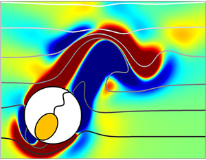
Figure 4. Normalized density difference ( $(\rho -\rho _0)/(\gamma {a})$) contours (isopycnals) for a pusher (
 $\beta =-3$) at different
  $Fr$. The lines with arrows are the streamlines in the frame of reference attached to the swimmer. A pusher entrains lighter density fluid in the vorticity bubble in its front. This results in a higher buoyancy force as it moves down in a heavier fluid and hence a reduction in its swimming speed. Stratification also leads to expansion of this vorticity bubble which means the vorticity generated at the pusher's surface cannot advect to the downstream as easily as it does in a homogeneous fluid. As a result, a pusher becomes unstable and the flow around it breaks axisymmetry in strong stratifications. The coordinate system is the same as in figure 1(c) and is hence not shown here.
  $(a)$
$(a)$  $Re=50$,
  $Fr \to \infty$.
  $(b)$
$(b)$  $Re=50$,
  $Fr=7$.
  $(c)$
$(c)$  $Re=50$,
  $Fr=5$.
  $(d)$
$(d)$  $Re=50$,
  $Fr=3$.
As the inertia of the pusher increases in a homogeneous fluid, the recirculatory region in front of it shrinks, leading to efficient downstream advection of the vorticity generated on its surface. As a result, its swimming speed increases with increasing the inertia in a homogeneous fluid. However, in a stratified fluid, the size of this recirculatory region increases as we increase the stratification (see figures 4 and 9). In addition, the pusher entrains the lighter fluid in this recirculatory bubble in front of it. So, as the pusher moves, it has to push this blob of the lighter fluid into a heavier fluid in front of it. This results in a higher buoyancy force opposite to the motion of a pusher reducing its swimming speed. Increasing the stratification strength increases the size of this blob of the lighter fluid in front of the pusher owing to the increase in the size of the recirculatory region. This effect can be seen by comparing the size of the lighter fluid blobs in front of the pushers in figures 4(b)–4(d) or the size of the vorticity bubbles in front of the pushers in figures 9(b)–9(d).
Unlike the pusher, a puller propels forward by ‘pulling’ the fluid in front and behind its body to its sides, as shown in the cartoon in figure 1(b). In a homogeneous fluid, the puller (shown by dashed lines in figure 1b) is pulled back by the flow field generated by itself at an earlier time (shown by solid lines in figure 1b). In addition, the fluid flow behind the puller obstructs the downstream advection of the vorticity generated on the pullers surface with increase in the inertia of the puller. The combined impact of these effects is the reduction in the puller's velocity as its inertia increases in a homogeneous fluid. Thus, any hindrance to the flow field generated by a puller in front and behind it will result in an inefficient downstream advection of the vorticity resulting in a slower swimming puller.
Similar to a pusher in a stratified fluid, the density stratification offers a significant resistance to generation of the flow field around a puller as it swims. This is because the puller has to pull the fluid packets in front and behind it from their neutrally buoyant positions to a region where the fluid packets experience a buoyancy force. e.g. the fluid which the puller pulls downwards behind it is lighter than the fluid it is getting pulled into, i.e. the fluid on the sides of the puller and vice versa for the fluid which the puller pulls upwards. Again, the hindrance to the flow-field generation by a puller can be visualized in terms of the deformations of the isopycnals around a puller at various stratification strengths. The isopycnals around a puller with increasing stratification are plotted in figure 5. The deformations in the isopycnals significantly reduce with increasing stratification strength, which becomes clear by comparing the deformations of the isopycnals in the wake of the pullers in figures 5(b)–5(d).

Figure 5. Normalized density difference ( $(\rho -\rho _0)/(\gamma {a})$) contours (isopycnals) for a puller (
 $\beta =3$) at different
  $Fr$. The lines with arrows are the streamlines in the frame of reference attached to the swimmer. A puller entrains lighter density fluid in the vorticity bubble in its rear. This results in a higher buoyancy force as it moves down or in a heavier fluid and hence a reduction in its swimming speed. A puller also pulls the heavier fluid around it upwards as it swims. These heavier isopycnals assist the swimming of the puller as they drag the puller with them while they try to resettle to their neutrally buoyant positions. Stratification also leads to contraction of this vorticity bubble size, which means the resistance to the vorticity advection to the downstream decreases as we increase stratification. As a result, a puller becomes stable and the flow around it remains axisymmetric even at high
  $Re$ for a strong stratification. The coordinate system is the same as in figure 1(c) and is hence not shown here.
  $(a)$
$(a)$  $Re=50$,
  $Fr \to \infty$.
  $(b)$
$(b)$  $Re=50$,
  $Fr=7$.
  $(c)$
$(c)$  $Re=50$,
  $Fr=5$.
  $(d)$
$(d)$  $Re=50$,
  $Fr=3$.
A puller entrains a lighter fluid in its rear recirculatory region. Thus, a puller has to drag this lighter blob of fluid with it as it moves into the heavier fluid below it. This results in a buoyancy force on the puller in the opposite direction to its motion resulting in a reduction in its swimming speed. But unlike the case of a pusher, the size of this recirculatory region behind a puller decreases with an increase in the stratification strength. This shrinkage can be seen by comparing the size of the lighter fluid blobs behind the pullers in figures 5(b)–5(d) or the size of the vorticity bubbles behind the pullers in figures 10(b)–10(d). As a result, the size of the blob of the lighter fluid that a puller has to pull with it also reduces, which is opposite to what happens in the case of a pusher moving in a stratified fluid. This explains the relatively lower reduction in the swimming speed of a puller than a pusher at the same  $Ri$.
$Ri$.
In addition to the squirmer speed, it is also interesting to look at the far-field velocity away from the squirmers. The far-field velocity for squirmers in a homogeneous fluid at  $Re=0$, i.e. in the absence of inertia, decays as
  $|w| \approx r^{-2}$. If the squirmers possess a finite inertia, then the fluid velocity in the swimming direction of the squirmers decays as
  $|w| \approx r^{-3}$ (Li et al. Reference Li, Ostace and Ardekani2016; Chisholm & Khair Reference Chisholm and Khair2018). We observe the same far-field flow structure in the squirmer swimming direction, i.e.
  $|w| \approx r^{-3}$, for the squirmers moving in a homogeneous fluid with a finite inertia, as shown in figure 6. Introducing stratification further hastens this decay with
  $r$ from the squirmer in the swimming direction, as shown in figures 6(a) and 6(b) for pushers and pullers, respectively. Figure 6 shows that the decay exponent of the far-field velocity in the swimming direction of the squirmers reduces significantly from
  $\approx -3$ in a homogeneous fluid to
  $\approx -10$ in a strongly stratified fluid with
  $Fr=1$. These results are consistent with previous studies which show that the effect of stratification is to suppress the vertical motion of the fluid (Ardekani & Stocker Reference Ardekani and Stocker2010; Doostmohammadi et al. Reference Doostmohammadi, Dabiri and Ardekani2014; More & Balasubramanian Reference More and Balasubramanian2018). The velocity field decays less rapidly for a pusher as compared to a puller at higher stratification strength owing to the increase in the vorticity bubble ahead of a pusher which expands as the stratification strength increases.

Figure 6. Effect of stratification on the far-field flow structure in the swimming direction of the inertial squirmers ( $Re=25$) with increasing stratification strength.
  $(a)$ Pusher with
  $\beta = -1$.
  $(b)$ Puller with
  $\beta =1$. Here,
  $r/a=1$ is at the velocity at the squirmer surface and increasing
  $r/a$ gives the locations in front of the squirmers in the downward direction along their axes (shown by dash-dotted lines in figure 1).
  $H$ in the legends stands for homogeneous fluid. The black solid lines are for comparison and show
  $r^{-3}$ and
  $r^{-10}$ decay. The velocity has been made dimensionless by the steady state squirmer speeds in a homogeneous fluid,
  $U_H$.
3.2. Strong stratification stabilizes a puller but destabilizes a pusher at intermediate  $Re$
$Re$

In a homogeneous fluid, a pusher is stable at high  $Re$ in the sense that the flow around it maintains a steady axisymmetry and it does not become unsteady three-dimensional as opposed to the flow around a puller which becomes unsteady three-dimensional at
  $Re \approx O(10)$ (Chisholm et al. Reference Chisholm, Legendre, Lauga and Khair2016; Li et al. Reference Li, Ostace and Ardekani2016). This breaking of the flow axisymmetry eventually makes the puller unstable beyond a critical
  $Re$. For the purpose of this study, we say that a squirmer is unstable once the axisymmetry of the flow around it breaks and it becomes unsteady.
A look at the flow fields around the squirmers predicts that the hydrodynamic interactions between the velocity fields induced by the inertial squirmers with their bodies is the reason behind these observations. An inertial puller (pusher) perturbed from its straight line trajectory is pushed away (pulled towards) the original trajectory due to these hydrodynamic interactions making it unstable (stable) at high  $Re$ (Li et al. (Reference Li, Ostace and Ardekani2016) and figure 1a,b). To gain further insight into why this is the case, we need to look at the vorticity field around a puller and a pusher. Pullers form a recirculatory region just behind them which is shown in figure 5(a) (streamlines are not shown inside the recirculatory region for the neatness of the plot). As we increase
  $Re$ for a puller, the size of this bubble increases. At some critical
  $Re$ determined by
  $\beta$, this bubble becomes so large that it hinders the convection of the vorticity produced on the surface of the squirmer to the downstream leading to instability and breaking the axisymmetry of the flow around the puller. On the contrary to pullers, pushers have the recirculatory region in front of them (figure 4a) and its size reduces with increasing
  $Re$. As a result, the vorticity produced on pusher's surface can be easily advected to the downstream making it eternally stable in a homogeneous fluid (figures 4a and 5a). We observe the same behaviour for pullers and pushers with high
  $Re$ in a homogeneous fluid. The puller fails to attain any steady velocity, becomes unsteady and suddenly follows a three-dimensional motion while a pusher is always steady in a homogeneous fluid (figures 8a and 8b for
  $Fr \to \infty$).
At intermediate  $Re$, we expect the puller to become stable at high enough stratification strengths and a pusher to be unstable at strong stratification strengths which is exactly opposite of what is observed in a homogeneous fluid. For an inertial squirmer in a stratified fluid, there are two competing effects which influence the stability of the squirmer: (i) the hydrodynamic interactions between the squirmer body and the flow field induced by its motion (inertial effect), and (ii) the resistance offered to the flow induced by the squirmers due to the exigency of the isopycnals displaced by the motion of the squirmer to resettle to their original positions (stratification effect). These two effects are competing because the flow field induced by the squirmers displaces the density stratified fluid around it in such a way that it has to go against the squirmer induced velocity field to return to its neutrally buoyant position, e.g. a pusher pushes the fluid around it downwards and upwards. As a result, these stratification effects offer resistance to the flow generated by the squirmers to propel themselves. The isopycnal that is pushed downwards (upwards) is flowing into a heavier (lighter) fluid, so as it tries to return to its original position, it has to flow opposite to the flow induced by the pusher.
In figure 7, we visualize the flow induced by the squirmers and the effect of stratification by arrows showing directions of the flows with their sizes indicating the strengths of these effects. For a puller (pusher) perturbed from its initial straight line trajectory, the inertial effect tries to push it away (pull it closer) while the stratification effect tries to pull it closer to (push it away from) the original trajectory. Consequently, for a particular  $Re$, at low enough
  $Fr$, the stratification effect wins, making the motion of the puller (pusher) stable (unstable). This is indeed true and can be seen easily in figures 8(a) and 8(b) which show that a puller which is unsteady in weak stratification becomes steady in strong stratifications and vice versa for a pusher.

Figure 7. Competition between the inertial and the stratification effects for a puller (a,b) and a pusher (c,d) in a weak and strong stratification. Curved arrows with filled heads (blue) denote the velocity fields induced by the squirmers (i.e. inertial effect) and arrows with hollow heads (red) denote the flow field induced by the exigency of the displaced isopycnals to return to their original position (i.e. stratification effect) at an earlier time, i.e. by the squirmer shown by solid lines. Sizes of the horizontal arrows on the perturbed squirmers show the relative magnitudes of these competing effects on the squirmer at the present time, i.e. on the squirmer shown by dotted lines. The laterally perturbed squirmer (denoted by dotted outline) is either attracted towards its original trajectory (b,c, stable squirmers) or is knocked away from the original trajectory (a,d, unstable squirmers) depending on the relative strength of these competing effects. Vertical arrows show the tendency of the squirmers to propel forward (blue) and the effect of stratification which hinders the forward propulsion of the squirmers (red). The vertical arrows are just for showing the directions of the respective effects and are not scaled. The flow-field description here is approximate and is not up to scale. The coordinate system is the same as in figure 1(c) and is hence not shown here.  $(a)$ Puller in weak stratification.
  $(b)$ Puller in strong stratification.
  $(c)$ Pusher in weak stratification.
  $(d)$ Pusher in strong stratification.

Figure 8. Effect of stratification on velocity history of squirmers. Swimming velocity evolution in vertical ( $U(t)$) and horizontal direction (
 $V(t)$) for a
  $(a)$ puller with
  $\beta$ = 3 and
  $(b)$ pusher with
  $\beta = -3$. Pullers become unstable and the flow around them becomes three-dimensional as we increase their inertia in a homogeneous fluid. Increasing stratification makes the motion of a puller steady and stable. On the other hand, a pusher is stable and the flow around it is axisymmetric for
  $Re$ as high as 1000 in a homogeneous fluid. Pushers are stable at low stratification strength, but become unstable for a strong stratification or at a large
  $Ri$. The other components of velocity remain 0 hence not shown.
  $(a)$
$(a)$  $Re=50$,
  $\beta =3$.
  $(b)$
$(b)$  $Re=50$,
  $\beta =-3$.
Stratification affects the stability of squirmers at finite  $Re$ in interesting ways compared to the homogeneous case, as discussed earlier. Pullers which are unstable in a homogeneous fluid at high
  $Re$ become stable and the flow around them remains axisymmetric for a high enough stratification. A puller with
  $\beta =3$ at
  $Re=50$ is unstable in a homogeneous fluid and for a weak stratification (
 $Fr=10$), but it becomes stable for higher stratifications (
 $Fr<8$) (see figure 8a). The effect of the stratification is to reduce the size of the vorticity bubble behind the pullers. The exigency of the heavier isopycnals pulled upwards by the puller to go back to their neutrally buoyant level is the reason behind this reduction in its size. This reduction in the recirculatory bubble size with increasing stratification is apparent from figures 5 and 10. Thus the advection of the vorticity produced at the puller's surface improves with increasing stratification which consequently makes the puller stable.
A pusher which is always stable in a homogeneous fluid for  $Re$ as high as 1000, however, becomes unstable at very strong stratification (See figure 8b) as the flow around it becomes unsteady three-dimensional. With increasing stratification, there are two mechanisms at play: (i) more rapid restoration of the disturbed isopycnals to their neutrally buoyant level, (ii) more entrainment of lighter fluid in the recirculatory region. For a particular
  $Re$, as we increase the stratification, both these effects lead to increase in resistance for the vorticity advection for a pusher, eventually breaking axisymmetry of the flow around it. This is because the size of the recirculatory region in front of a pusher increases as more lighter fluid is trapped (see figure 4). In addition, the need of the isopycnals to go back to their original level in the downstream of the pusher results in lateral expansion of the vorticity wake behind it (see figure 9).

Figure 9. Effect of stratification on the vorticity field around a pusher with  $\beta =-3$. Colour bar shows the
  $y$-vorticity value. Increasing stratification leads to accumulation of the vorticity in front of a pusher which hinders the advection of vorticity generated in the front part of a pusher to the downstream. Panel (a) shows the vorticity advection in a homogeneous fluid and hence isopycnals are not shown. In (b–d) the solid lines denote density differences compared to the reference density
  $\rho _0$ and normalized by
  $\gamma {a}$, i.e.
  $({\rho - \rho _0})/{\gamma {a}}$. Spacing between the lines is 1 unit and darker shade of grey denotes higher density value. The coordinate system is the same as in figure 1(c) and is hence not shown here.
  $(a)$
$(a)$  $Re=50$,
  $Fr \to \infty$.
  $(b)$
$(b)$  $Re=50$,
  $Fr = 7$.
  $(c)$
$(c)$  $Re=50$,
  $Fr = 5$.
  $(d)$
$(d)$  $Re=50$,
  $Fr=3$.
Figures 4, 5 and 9, 10 reveal the similarity between the flow fields generated by the motion of a bubble (Bayareh et al. Reference Bayareh, Doostmohammadi, Dabiri and Ardekani2013) and a rigid sphere (Doostmohammadi et al. Reference Doostmohammadi, Dabiri and Ardekani2014) in a stratified fluid with the flow fields around pushers and pullers, respectively. This resemblance in the corresponding flow fields generated by a pusher and a puller with that of a inviscid spherical bubble and a rigid towed sphere is also observed in the case of a homogeneous fluid (Chisholm et al. Reference Chisholm, Legendre, Lauga and Khair2016). A rising bubble and a pusher have a mobile surface which causes the advection of the vorticity downstream. This avoids formation of any wake eddy in the downstream flow of a pusher giving it a long trailing vorticity wake which is similar to that of a rising bubble. On the other hand, the trailing vorticity wake bubble in the case of a puller is similar to the vorticity field behind a settling rigid sphere in a stratified fluid. This is caused by the reversal of the tangential surface velocity of the pusher and is akin to the effect caused by the no-slip boundary condition on the surface of the settling sphere.

Figure 10. Effect of stratification on the vorticity field around a puller with  $\beta =3$. Colour bar shows the
  $y$-vorticity value. Increasing stratification leads to shrinking of the vorticity bubble behind the puller, which facilitates the advection of vorticity to the downstream. Panel
  $(a)$ shows the vorticity advection in a homogeneous fluid and hence isopycnals are not shown. For (b–d) the solid lines denote density differences compared to the reference density
  $\rho _0$ and normalized by
  $\gamma {a}$, i.e.
  $({\rho - \rho _0})/{\gamma {a}}$. Spacing between the lines is 1 unit and darker shade of grey denotes higher density value. The coordinate system is the same as in figure 1(c) and is hence not shown here.
  $(a)$
$(a)$  $Re=50$,
  $Fr \to \infty$.
  $(b)$
$(b)$  $Re=50$,
  $Fr=7$.
  $(c)$
$(c)$  $Re=50$,
  $Fr=5$.
  $(d)$
$(d)$  $Re=50$,
  $Fr=3$.
Figure 11 summarizes the stable–unstable squirmer motion for all the  $Re$–
$Re$– $Fr$ values explored in this study. We observe that, if a puller is stable in a homogeneous for a given
  $Re$, it remains stable in a stratified fluid too (pullers with low
  $|\beta |$, e.g.
  $\beta =1$). However, at higher
  $\beta$, pullers become unstable in a homogeneous fluid for
  $Re \approx O(10)$. We observed that, at high
  $Re$, the pullers are unstable in a homogeneous fluid and weak stratifications, but gradually their motion transitions to a steady state as we increase the stratification. Thus, if a puller is unstable at a particular
  $Re$ in a homogeneous fluid, it remains unstable in weak stratifications for the same
  $Re$ but becomes stable if stratification is sufficiently strong. But the critical stratification strength required for a puller to be stable increases with
  $Re$. For the pushers, we observed that, the instability in their motion ensues for
  $Fr \lessapprox 1$ for
  $Re>5$ explored in this study.
  $Fr$ gives the relative magnitude of the inertial forces with the buoyancy forces due to the displacement of the isopycnals. So, it is expected that as
  $Fr \lessapprox 1$, a pusher becomes unstable due to the increase in the relative importance of the destabilizing effects due to the density stratification. Also, the finite time required for the onset of instability from the initial time (as can be seen in figure 8) is due to the time required for the flow solver to reach a solution where initial transients in the velocity field die down. This is consistent with previous studies in a homogeneous fluid (Chisholm et al. Reference Chisholm, Legendre, Lauga and Khair2016; Li et al. Reference Li, Ostace and Ardekani2016). The onset of path/wake instabilities in a settling no-slip sphere also require a finite time which is expected as it takes some time for the flow field to fully develop (Rahmani & Wachs Reference Rahmani and Wachs2014).

Figure 11. A polar phase diagram indicating the effect of stratification and inertia on the stability of the squirmers. Open symbols ( $\triangle$) indicate stable squirmer motion, while filled symbols (
 $\blacktriangle$) indicate unstable squirmer motion. Each quarter (separated by dash-dotted lines) is for a fixed
  $\beta$ value indicated by legends in the corners. The black dotted lines separate the stable cases from the unstable ones. Each quarter is for a fixed
  $\beta$ squirmer. Each circle (radial direction) represents a constant
  $Fr$ value which increases as we go outward. The innermost circle is the maximum stratification strength while the outermost circle is for a homogeneous fluid. A fixed polar coordinate represents a fixed
  $Re$ with values indicated on the outermost circle.
3.3. Swimming and mixing efficiency
For a body moving in a linearly stratified fluid, the energy equation in a quasi steady state can be written as
 \begin{equation} \mathcal{P} = \oint_S \left( \boldsymbol{u} \boldsymbol{\cdot} \boldsymbol{\boldsymbol\sigma} \right) \boldsymbol{\cdot} \boldsymbol{n} \,\textrm{d}S = \int_{\varOmega - \varOmega_s} 2\mu\boldsymbol{E}:\boldsymbol{E} \,\textrm{d}\varOmega - \int_{\varOmega-\varOmega_s} w\rho'g \,\textrm{d}\varOmega, \end{equation}
where  $\boldsymbol {\sigma }$ is the stress tensor,
  $S$ is the squirmer's surface,
  $\boldsymbol {n}$ is the normal unit vector to
  $S$,
$S$,  $\boldsymbol {E}$ is the strain rate tensor,
  $\rho '$ is the perturbation from the initial linear background density
  $\rho _f$ and
  $\varOmega _s$ is the squirmer domain, i.e.
  $\phi =1$. The first term on the right-hand side is the viscous dissipation (
 $\varPhi$) over the entire fluid domain while the second term is the rate of creation of the gravitational potential energy (
 $\Delta {PE}$). Together, these two terms give us the energy expended by the squirmer for its locomotion in a linearly stratified fluid in a steady state. The energy expended by the squirmer for its steady state motion is dissipated in the form of mechanical energy in the surrounding fluid and hence can be calculated as in (3.2).
The swimming efficiency ( $\eta _e$) of the squirmers is defined as the ratio of the power necessary to move the spherical squirmer body (
 $\mathcal {P}^{*} = 6{\rm \pi} \mu {U}^2a(1+3/8Re)$) at its swimming speed
  $U$ to the power expended by the squirmer
  $\mathcal {P}$ (Wang & Ardekani Reference Wang and Ardekani2012a)
 \begin{equation} \eta_e = \frac{\mathcal{P}^{*}}{\mathcal{P}}. \end{equation}
Figure 12(a) shows the swimming efficiency of the squirmers in a stratified fluid at a constant  $Re=25$. Earlier studies for the motion of an inertial squirmer in a homogeneous fluid observed that a pusher is more efficient than puller (Wang & Ardekani Reference Wang and Ardekani2012a) which is also true in a stratified fluid. In addition, increasing the magnitude of
  $|\beta |$ results in a reduction in the swimming efficiency. The viscous dissipation as well as the gravitational potential energy generation increases with increasing
  $|\beta |$ resulting in a lower swimming efficiency. This is expected as the gradients in the velocity as well as the magnitude of density perturbations increase with the squirmer
  $|\beta |$ value. This observation is consistent with earlier studies in an inertial regime but in a homogeneous fluid (Wang & Ardekani Reference Wang and Ardekani2012a).

Figure 12.  $(a)$ Effect of stratification on the swimming efficiency of the squirmers for swimming. Here,
  $\mathcal{P}^{\ast} = 6{\rm \pi} \mu {U}^2{a} ( 1 + 3/8Re )$ (Wang & Ardekani Reference Wang and Ardekani2012a), which is the power required to tow the squirmer body in a homogeneous fluid at the same
  $Re$ and the velocity
  $U$.
$U$.  $(b)$ Effect of stratification on the mixing efficiency (
 $\varGamma$) of squirmers.
  $Re=25$ for both plots. Open symbols: pullers. Filled symbols: pushers.
A pusher observes a higher reduction in its swimming velocity in a stratified fluid with respect to its swimming velocity in a homogeneous fluid than a puller for the same  $Re$ and
  $Fr$, as discussed in § 3.1. Still, a pusher swims faster than a puller for the same
  $Re$ and
  $Fr$ values (see figure 2). This is due to the effective vorticity advection by the flow field around a pusher as compared to a puller. As can be seen by comparing figures 9 and 10, pushers have a long wake behind them which indicates the efficient vorticity advection downstream. However, the wake becomes shorter with increasing the stratification for a puller signifying resistance to the vorticity advection downstream. This is also the reason why a pusher swims more efficiently that a puller in a stratified fluid for the same
  $Re$ and
  $Fr$ values. Furthermore, with increasing the stratification, the
  $\Delta {PE}$ increases by 1–2 orders of magnitude while
  $\varPhi$ increases only slightly. Thus, as the stratification increases, more energy is expended by the squirmer in
  $\Delta {PE}$, resulting in the lowering of its swimming efficiency with increase in the stratification strength.
The mixing efficiency ( $\varGamma$), which is the ratio of the potential energy generated to the total energy expended in producing the mixing, is an important parameter to quantify the mixing generated by bodies in a stratified fluid. It can be defined as
 \begin{equation} \mathcal{\varGamma} = \frac{- \int_{\varOmega-\varOmega_s} w\rho'g \,\textrm{d}\varOmega}{\oint_{\varOmega-\varOmega_s} \left( \boldsymbol{u} \boldsymbol{\cdot} \boldsymbol{\sigma} \right) \boldsymbol{\cdot} \boldsymbol{n} \,\textrm{d}S} = \frac{- \int_{\varOmega-\varOmega_s} w\rho'g \,\textrm{d}\varOmega}{ \int_{\varOmega-\varOmega_s} 2\mu\boldsymbol{E}:\boldsymbol{E} \,\textrm{d}\varOmega - \int_{\varOmega-\varOmega_s} w\rho'g \,\textrm{d}\varOmega}. \end{equation}
The mixing efficiency induced by organisms has been an active area of study in the recent years (Dewar et al. Reference Dewar, Bingham, Iverson, Nowacek, St Laurent and Wiebe2006; Visser Reference Visser2007; Katija & Dabiri Reference Katija and Dabiri2009; Katija Reference Katija2012; Wang & Ardekani Reference Wang and Ardekani2015; Dandekar et al. Reference Chisholm, Legendre, Lauga and Khair2019; Kunze Reference Kunze2019). Thus, looking at the mixing efficiency of an individual swimmer can help us in understanding the mixing produced by a school of swimmers. Figure 12(b) gives the mixing efficiency for pushers and pullers at various  $Ri$ and shows that increasing stratification increases the mixing efficiency for both pushers and pullers. A pusher (puller) with higher magnitude of
  $\beta$ has a larger mixing efficiency. This is obvious as a squirmer with higher
  $|\beta |$ has a higher velocity leading to higher vertical mass flux and hence achieves larger mixing.
The mixing efficiency induced by an individual micron size microorganism in a marine environment is  $O(10^{-8})$ (Wagner, Young & Lauga Reference Wagner, Young and Lauga2014) which means in absence of swimmer inertia, its motion does not lead to any significant mixing. Wang & Ardekani (Reference Wang and Ardekani2015) calculated
  $\varGamma$ for a swarm of squirmers at finite inertia. They observed that
  $\varGamma$ increases with
  $Re$ and the squirmer concentration. They also observed that, at a lower
  $Ri$, a puller exhibits higher
  $\varGamma$ while at a high value of
  $Ri$, a pusher has higher
  $\varGamma$. However, it is not clear why the mixing efficiency increases with increasing
  $Ri$ for the swarm of squirmers. The reason for this becomes clear if we look at the mixing efficiency generated by individual squirmers in figure 12(b). At low
  $Ri$ (
 $<2$), the mixing efficiency is more for a puller compared to a pusher with the same
  $Re$ and
  $\beta$. However, at higher
  $Ri$ (
 $>2$), pusher has a higher
  $\varGamma$ than a puller. This trend in
  $\varGamma$ at the individual level of the squirmers is what leads to the same behaviour for a swarm of squirmers.
As mentioned before, we observed that, with increasing the stratification, the  $\Delta {PE}$ increases by 1–2 orders of magnitude while
  $\varPhi$ increases only slightly. Also, the calculations show that
  $\varPhi \gg \Delta {PE}$. Thus, we can conclude that it is the numerator term that governs the behaviour of the mixing efficiency generated by a single squirmer moving in a stratified fluid. Hence, to explain the trends in
  $\varGamma$, we plot the gravitational potential energy generated, i.e. the numerator term in (3.4). As can be seen in figure 13, most of the gravitational potential energy is generated in the recirculatory regions of the squirmers. With increasing the stratification, the amount of
  $\Delta {PE}$ generated by a puller (can be seen by maximum
  $\Delta {PE}$ value in the contours) increases significantly but the size of its recirculatory region also decreases. However, this increase in the amount of
  $\Delta {PE}$ generated by a puller is significantly higher (
 $\approx$4 folds) than the shrinking (
 $\approx$2 folds) of its rear recirculatory region as can be seen in figures 13(a) and 13(c). This results in the higher
  $\varGamma$ at higher
  $Ri$ for a puller. On the other hand, with increasing stratification strength, the size of the recirculatory region as well as the amount of
  $\Delta {PE}$ generated by a pusher increase, as can be seen from figures 13(b) and 13(d). Thus, the
  $\varGamma$ by a pusher also increases with increase in the stratification strength of the background fluid.

Figure 13.  $\Delta{PE}$ contours depicting the effect of stratification on the gravitational potential energy generated by squirmers at low and high stratification strengths for
  $Re=25$. Potential energy is generated mainly in the recirculatory regions of pushers and pullers. The coordinate system is the same as in figure 1(c) and is hence not shown here.
  $(a)$
$(a)$  $Fr = 10, \beta = 3$.
  $(b)$
$(b)$  $Fr=10,\, \beta =-3$.
  $(c)$
$(c)$  $Fr=3, \beta =3$.
  $(d)$
$(d)$  $Fr=3, \beta =-3$.
The switching in the relative magnitudes of  $\varGamma$ for a puller and a pusher for
  $Ri > 2$ can also be explained by looking at the
  $\Delta {PE}$ contours in figure 13. At low
  $Ri$ values, i.e. high
  $Fr$ values (figures 13a and 13b), the puller generates more
  $\Delta {PE}$ compared to a pusher owing to the bigger size of its recirculatory region. However, this scenario changes completely with increasing the stratification strength. At high
  $Ri$ values, i.e. low
  $Fr$ values (figures 13c and 13d), the recirculatory region behind a puller shrinks while the recirculatory region in front of the pusher gets bigger as compared to the lower
  $Ri$ case. In addition, the amount of
  $\Delta {PE}$ (can be seen by comparing the maximum
  $\Delta {PE}$ value in the contours), also increases significantly for a puller as compared to a pusher at high stratification strengths. This results in the higher
  $\varGamma$ for a pusher than a puller at high
  $Ri$ values as shown in figure 12(b). We observed similar trends for other
  $Re$ values investigated in this study as well.
4. Conclusions
We present a direct numerical simulation study on the locomotion of a single neutrally buoyant swimmer with finite inertia in a linearly stratified fluid. For modelling the swimmer locomotion mechanism, we use the reduced squirmer model which produces propulsion by periodic deformations of an array of cilia present on its surface. The problem of self-propulsion of such a squirmer with finite inertia in a linearly stratified fluid is more complex than a squirmer moving in a homogeneous fluid. This complexity gives rise to interesting phenomena and significantly changes the motion of squirmers as compared to their movement in a homogeneous fluid.
We use the Richardson number  $Ri = Re/Fr^2$ to quantify the stratification strength. We observe that, irrespective of the value of
  $\beta$, stratification leads to reduction in the steady state swimming speed for squirmers. The reason for this is the trapping of lighter density fluids in the recirculatory regions by the pullers (
 $\beta >0$) and the pushers (
 $\beta <0$). This results in a buoyancy force on the squirmers in the opposite direction to their swimming motion which reduces their swimming speed. In addition, the resistance offered by the isopycnals to their deformation due to the flow fields generated by the squirmers increases with increasing stratification. This also results in the reduction of the swimming speeds of the squirmers.
Another significant deviation from the homogeneous case is regarding the stability of the squirmers. The flow around the pullers become unsteady three-dimensional at high  $Re$, making them unstable, while pushers remaining stable for very high
  $Re$ in a homogeneous fluid. The reason for this is the increasing size of the recirculatory region in the rear of the pullers with
  $Re$ which hinders the vorticity advection to the downstream, causing the instability, while the recirculatory region in front of the pushers shrinks with increasing inertia leading to an efficient vorticity advection to the downstream, making them eternally stable. The effect of stratification is exactly the opposite from the effect of inertia. Stratification leads to shrinking of the rear recirculatory bubble for a puller as a puller ‘pulls’ heavier fluid from its sides upwards. In the exigency by these heavier isopycnals to move to their neutrally buoyant level that leads to shrinking of the vorticity bubble behind the pullers. On the contrary, stratification leads to the expansion of the front recirculatory bubble of a pusher as it ‘pushes’ lighter fluid trapped in front of it to heavier fluid. So high enough stratification makes a puller stable while a very strong stratification breaks the axisymmetry of the flow around a pusher making it unstable.
The energy calculations for a pusher and a puller show that a pusher is more efficient at swimming in a stratified fluid as compared to a puller considering the differences in their swimming speeds. Again, the efficient advection of the vorticity to the downstream by the pushers is the reason for this trend. The mixing efficiency of the puller is higher at low  $Ri$ (
 $<2$) while the mixing efficiency of a pusher is higher at high
  $Ri$ (
 $>2$). The reason for this is the similar trend in the generation of the gravitational potential energy by pullers and pushers in the respective
  $Ri$ regimes.
These results hint towards the fascinating role of density stratification on the locomotion of marine organisms like ciliary zooplanktons and provide possible clues for the reasons behind the preferential accumulation of larger sized planktons at pycnoclines (Viličić et al. Reference Viličić, Legović and Žutić1989). The speed of larger organisms with higher inertia, when they encounter a density jump or a strong stratification during the vertical migratory motion in oceans, significantly reduces and the energy required for the propulsion also goes up. In addition, the swimmers stray from their straight vertical trajectory and start swimming in the horizontal direction due to the onset of instability (e.g. high  $Re$ pullers in a weak stratification or a pusher in a very strong stratification). This might lead to the accumulation of the swimmers at the density interface. These mechanisms come into play only at a finite
  $Re$. At low
  $Re$, the swimmers are always stable (Chisholm et al. Reference Chisholm, Legendre, Lauga and Khair2016; Li et al. Reference Li, Ostace and Ardekani2016) and stratification might lead to increase in their speeds, e.g. pullers (Doostmohammadi et al. Reference Doostmohammadi, Stocker and Ardekani2012), thus resulting in negligible accumulation which is true for smaller sized planktons (Viličić et al. Reference Viličić, Legović and Žutić1989). Stratification also increases the mixing efficiency generated by an individual swimmer, an effect which amplifies when we consider swarms of swimmers (Wang & Ardekani Reference Wang and Ardekani2015; Houghton et al. Reference Houghton, Koseff, Monismith and Dabiri2018).
Even though these organisms dwell in a density stratified environment, most of the experimental studies on their locomotion have been done in a homogeneous fluid. More experimental studies are thus needed to investigate the effect of stratification on the motion and flow fields of individual marine organisms. In addition, real marine organisms have a wide variety of shapes, create jets as they swim and show a wide variety of other variations. Studying the effect of these variations on the swimming dynamics of organisms in a stratified fluid is also an interesting problem to investigate.
Acknowledgements
The authors would like to acknowledge financial support from the National Science Foundation via grants CBET-1604423, CBET-1700961 and CBET-1705371 to A.M.A. This work used the Extreme Science and Engineering Discovery Environment (XSEDE) (Towns et al. Reference Towns, Cockerill, Dahan, Foster, Gaither, Grimshaw, Hazlewood, Lathrop, Lifka and Peterson2014), which is supported by the National Science Foundation grant number ACI-1548562 through allocations TG-CTS180066 and TG-CTS190041. R.V.M. would like to thank S. Wang, N. Desai, V. Shaik and R. Dandekar for insightful discussions.
Declaration of interests
The authors report no conflict of interest.
Supplementary movie
Supplementary movie is available at https://doi.org/10.1017/jfm.2020.719.
Appendix A. Grid and domain independence
This appendix is dedicated to the grid and domain independence tests of the computer program utilized for this study.
Figure 14(a) shows the effect of three grid sizes with 70 grid points per diameter, 35 grid points per diameter and 25 grid points per diameter on the velocity evolution of a pusher with  $\beta =-1$ moving at
  $Re=25$. The change in the swimming speed from 25 grid points to 35 grid points is 5.2 % which reduces to 1.5 % from 35 grid points to 70 grid points per diameter. So we run all the simulations for a grid size with 35 grid points per squirmer diameter in all the cases.

Figure 14.  $(a)$ Grid independence test for three different grid sizes. The plot shows
  $z$-velocity evolution for a pusher with
  $\beta =-1$ at
  $Re=25$.
  $(b)$ Domain independence test for two different grid sizes. The plot shows
  $z$-velocity evolution for a pusher with
  $\beta =-1$ at
  $Re=25$ and
  $Fr=5$.
  $(a)$ Grid independence.
  $(b)$ Domain independence.
Figure 14(b) shows the effect of changing the domain size. We tested two domain sizes  $4.5d \times 4.5d \times 40d$ and
  $9d \times 9d \times 80d$. The results are the same for both the domain sizes with less than 0.1 % deviation. Hence we run all the simulations for a domain size
  $9d \times 9d \times 80d$.
Additional validations can be found in Doostmohammadi et al. (Reference Doostmohammadi, Dabiri and Ardekani2014) (for the dynamics of a spherical object in a linearly stratified fluid) and Li et al. (Reference Li, Ostace and Ardekani2016) (for the dynamics of inertial squirmers in a homogeneous fluid).
Appendix B. Effect of Prandtl number
This study investigated the locomotion of a squirmer in a linearly stratified fluid with the fluid having a  $Pr = 0.7$. This was done in order to resolve the density boundary layer without making the simulations computationally too expensive. Here, we present results for
  $Pr = 7$ and compare them with the results for
  $Pr=0.7$. It has been shown for the case of a spherical object settling in a linearly stratified fluid, changing the
  $Pr$ only changes the magnitudes of the flow variables with their behaviour and trends being similar (Doostmohammadi et al. Reference Doostmohammadi, Dabiri and Ardekani2014). We expect similar effect of changing
  $Pr$ on the motion of a squirmer as well.
Figure 15 shows that increasing  $Pr$ changes the magnitude of steady state swimming velocities but the overall behaviour of the velocity time history is similar in both cases. The plot shows that squirmer velocity does not experience a notable change before reaching the maximum value after which it attains a smaller steady state swimming speed at higher
  $Pr$. These observations are similar to the effect of changing
  $Pr$ in the case of a sphere settling in a linearly stratified fluid (Doostmohammadi et al. Reference Doostmohammadi, Dabiri and Ardekani2014). The effect of stratification on the swimming speed of a squirmer is similar at higher
  $Pr$, i.e. stratification reduces the swimming speed of squirmers.

Figure 15. Effect of  $Pr$ on the velocity evolution of the squirmers. Changing
  $Pr$ merely changes the magnitude of the velocity but the overall behaviour for the velocity is the same. This observation is similar to the effect of changing
  $Pr$ on a rigid sphere settling in a stratified fluid. This plot shows even at a higher
  $Pr$ increasing stratification reduces the swimming speed.
Appendix C. Locomotion of non-neutrally buoyant squirmers in a stratified fluid and the validity of the Boussinesq approximation
In this appendix, we present the motion of non-neutrally buoyant squirmers and the validity of using the Boussinesq approximation in (2.1). Figure 16(a) shows the swimming speed evolution of a pusher and a puller in a homogeneous and a stratified fluid with  ${Fr=3}$. The squirmers are not neutrally buoyant in this plot. They have
  $\rho _s/\rho _0 = 1.04$. Please note that
  $\rho _0 = \rho _f$ in a homogeneous fluid. As a result of this, they experience a buoyancy force in the direction of their motion due to the density difference with the background fluid. In a homogeneous fluid, this density difference leads to a higher swimming speed of the squirmers compared to their swimming speeds when
  $\rho _s/\rho _0 = 1$. In a stratified fluid, the squirmer velocity increases first, reaching a maximum and it decreases gradually after that to become 0 when the squirmers reach their neutrally buoyant positions.

Figure 16.  $(a)$ Swimming speed evolution of non-neutrally buoyant squirmers with
  $\rho _s/\rho _0 = 1.04$ with
  $Re = 15.6$ in a homogeneous fluid (
 $H$) and a stratified fluid with
  $Fr=3$. The squirmers were initialized at a distance
  $40d$ above their neutrally buoyant positions (i.e.
  $z$ at which
  $\rho (z)=\rho _s$).
  $(b)$ Validity of Boussinesq approximation. The plot shows the swimming speed evolution for a pusher with (red
  $\Diamond$) and without (red dashed line,
  $\boldsymbol {--}$) the Boussinesq approximation as well as for a puller with (blue
  $\square$) and without (blue solid line,
  $\boldsymbol {-}$) the Boussinesq approximation. Here,
  $|\beta |=3$,
  $Re=25$ and
  $Fr=5$.
If the swimmers are not neutrally buoyant, they have a different density compared to the background fluid. This means that they have two main contributions which determine their swimming speeds: (i) their self-propulsion due to the surface velocity and (ii) the settling/rising motion due to the difference in density with the background fluid. If the swimmers are close to their neutrally buoyant level (z such that  $\rho(z) = \rho_s$) in the fluid, i.e. the depth of the fluid where the fluid density is equal to the squirmer density, then we expect them to swim till they reach their neutrally buoyant level where they might either oscillate or stop or get deflected in the horizontal direction depending on their
  $\beta$ and the stratification strength. This kind of mechanism might be leading to the accumulation of phytoplanktons in the oceans. In all these cases, they get trapped at their neutrally buoyant levels due to the reduction of their vertical swimming velocity to
  $\approx 0$. This is similar to what happens in the case of a heavy sphere settling (Doostmohammadi et al. Reference Chisholm, Legendre, Lauga and Khair2014) or a drop rising (Bayareh et al. Reference Chisholm, Legendre, Lauga and Khair2013) in a stratified fluid. Their settling/rising velocity gradually decreases and becomes 0 as they reach their neutrally buoyant levels. If the swimmers are far away from their neutrally buoyant levels, then there is a huge difference in the fluid and swimmer density resulting in a motion similar to settling of a passive sphere. This means that the squirmers do not attain a steady state velocity. Thus, in any of these cases, we do not expect the squirmers to reach a steady velocity.
For the results presented in this paper, we have assumed the Boussinesq approximation is valid in the Navier–Stokes equations (2.1). The validity of using the Boussinesq approximation in the case of a settling no-slip sphere is presented in Doostmohammadi et al. (Reference Doostmohammadi, Dabiri and Ardekani2014). To test this assumption for squirmers for the range of parameters in this paper, we present the comparison of the velocity evolution for a pusher and a puller with  $|\beta |=3$ and
  $Re=25$ in a stratified fluid with
  $Fr=5$ in figure 16(b). The plot shows that there is only a small change in the squirmer velocity if we relax the Boussinesq approximation. The solution with the Boussinesq approximation slightly under-predicts the swimming velocity for the squirmers. These results show that the Boussinesq approximation is valid in the present study.
Appendix D. Effect of squirmer orientation
The results presented in the manuscript are for squirmers swimming downwards, i.e. parallel to the direction of the gravity and in a heavier fluid. However, in reality, they might swim in various other orientations too. So, in this appendix we present swimming speed evolution for squirmers with  $Re=50$ in other orientations. The other orientations considered are: (i) opposite to the direction of gravity, or vertically upwards, (ii) perpendicular to the direction of gravity or horizontal. In both these cases, the qualitative behaviour of the squirmer swimming is similar, as shown in figures 17(a) and 17(b).

Figure 17.  $(a)$ Swimming speed evolution of squirmers with initial orientations vertically down (direction of gravity) and up (opposite to the direction of gravity), respectively. Here,
  $Re=25$ and
  $|\beta |=3$. Hollow symbols and solid lines represent pushers while filled symbols and dotted lines represent pullers.
  $(b)$ Swimming speed evolution of squirmers with initial orientations horizontal (perpendicular to the direction of gravity). Here,
  $Re=50$ and
  $|\beta |=3$. Increasing the stratification reduces the swimming speed of the squirmers but this reduction is small compared to the case when they move in the direction of gravity.
Figure 17(a) shows the swimming speed evolution for a puller and a pusher with  $|\beta |=3$ and
  $Re=25$ at two different
  $Fr$ moving parallel to (downward) and opposite to (upward) the direction of the gravity. The swimming speed evolution is similar in both cases. The squirmer swimming speed decreases with increasing the stratification compared to its swimming speed in a homogeneous fluid even if it is moving opposite to the direction of gravity. We observe that, the squirmer swimming upward in a stratified fluid has slightly smaller velocity that the same squirmer swimming downward for the same conditions.
Figure 17(b) shows the swimming speed evolution for a pusher and a puller with  $|\beta |=3$ and
  $Re=50$ in a homogeneous fluid and a stratified fluid with two different
  $Fr$ moving in a direction perpendicular to the direction of gravity, i.e. horizontal. Increasing the stratification decreases the swimming speed of the squirmers compared to their speeds in a homogeneous fluid. But this reduction is small compared to the case when they move vertically. In addition, the stratification does not stabilize a puller even in a strongly stratified fluid at high
  $Re$ if it moves in the horizontal direction.