2.1. Governing equations

The time-dependent reactive Euler equations are employed to numerically solve two-dimensional (2-D) gaseous detonation with convective and reactive effects, as follows:

(2.1) \begin{align} \displaystyle \frac {\partial \boldsymbol {Q}}{\partial t}+ \boldsymbol {\nabla} \boldsymbol {\cdot }(\boldsymbol {F})= \boldsymbol {S}, \end{align}

where $\boldsymbol {Q}$, $\boldsymbol {F}$ and $\boldsymbol {S}$ represent the vector of conserved variables of the solution, the face flux vector corresponding to the conserved variables and the source vector, respectively. The details of these vectors are expressed as follows:

(2.2a-c) \begin{align} \boldsymbol {Q} = \left [ \begin{array}{c@{\quad}c@{\quad}c@{\quad}c@{\quad}c} \rho Y_1 \\[3pt] \displaystyle \vdots \\[3pt] \rho Y_N \\[3pt] \rho \boldsymbol {U} \\[3pt] \displaystyle \rho E \\[3pt] \end{array} \right ] ,\quad \boldsymbol {F} = \left [ \begin{array}{c@{\quad}c@{\quad}c@{\quad}c@{\quad}c} \rho Y_1 \boldsymbol {U} \\[3pt] \displaystyle \vdots \\[3pt] \rho Y_N \boldsymbol {U} \\[3pt] \rho \boldsymbol {U} \boldsymbol {U} + p \\[3pt] \displaystyle \rho E \boldsymbol {U} + \boldsymbol {U} p \\[3pt] \end{array} \right ] ,\quad \boldsymbol {S} = \left [ \begin{array}{c@{\quad}c@{\quad}c@{\quad}c@{\quad}c} \omega _1 \\[3pt] \displaystyle \vdots \\[3pt] \omega _N \\[3pt] 0 \\[3pt] \displaystyle \omega _{{T}} \\[3pt] \end{array} \right ], \end{align}

where $N$ is the total number of species, $\rho$ is the total density of the mixture, $Y_k (k = 1, \ldots , N)$ is the mass fraction of the $k$th species, $\sum _{k=1}^N(Y_k)=1$, $\boldsymbol {U} = (u_x, u_y, u_z)^{\mathrm {T}}$ is the velocity vector ($u_y$ always equals zero for the 2-D case of present work), $p$ is the pressure and $E$ is the total energy without chemical energy, which is calculated by

(2.3) \begin{align} E = h_{{s}}-\frac {p}{\rho }+\frac {1}{2} \Vert \boldsymbol {U} \Vert ^2. \end{align}

The sensible enthalpy $h_{{s}}$ in the above equation is evaluated by the seven-coefficient polynomial from the JANAF tables (Chase et al. Reference Chase, Curnutt, Prophet, McDonald and Syverud1975). The equation of state for a thermally perfect gas is utilized to close the system of governing equations. The source term $\omega _k$ of the $k$th species equation represents the formation/consumption rate of the $k$th species, and is determined by the law of mass action. The source term $\omega _{{T}}$ of the energy equation in (2.2) is the rate of reaction heat release, and is expressed as

(2.4) \begin{align} \displaystyle \omega _{{T}} = \sum _{k=1}^N \omega _k \Delta h_{{f},k}^{\circ }, \end{align}

where $\Delta h_{{f},k}^{\circ }$ is the formation enthalpy of the $k$th species.

2.2. Numerical methods

Based on an unstructured grid and finite volume framework, the adaptive mesh refinement framework available within OpenFOAM (Jasak Reference Jasak1996) is employed for discretizing the computational domain, and the refinement criterion is set based on the density gradient, which is an indicator of not only the shock wave but the contact discontinuity. The time terms in the governing equations are processed via a second-order total variation diminishing (TVD) RungeKutta scheme with the time step being dictated by the Courant–Friedrichs–Lewy (CFL) number, which is set to 0.3 for all computations undertaken in this study. The convection term $\boldsymbol {F}$ is approximated using a second-order central-upwind scheme (Kurganov, Noelle & Petrova Reference Kurganov, Noelle and Petrova2001) that proficiently pinpoints the location of various discontinuities in the flow field. Hence, this scheme is widely used in the study of detonations (Gutiérrez Marcantoni et al. Reference Gutiérrez Marcantoni, Tamagno and Elaskar2017; Guo et al. Reference Guo, Xu, Zheng and Zhang2023). A detailed hydrogen combustion reaction mechanism (listed in Appendix A) proposed by Burke et al. (Reference Burke, Chaos, Ju, Dryer and Klippenstein2012) is used to model the chemical reactions due to its special treatment of hydrogen combustion under high-pressure conditions. The source terms $\omega _k$ for the chemical reactions are solved using the Euler point-implicit method in the present study, effectively reducing the stiffness associated with the system of ordinary differential equations.

2.3. Computational configurations

To conduct the numerical simulation of the detonation wave in a 2-D channel, the shock-fixed frame is used, as shown in figure 2. We used two different mixtures, i.e. the stoichiometric H$_2$/air and the stoichiometric H$_2$/O$_2$ mixtures, and the computational conditions for both mixtures are listed in table 1. To understand the temperature sensitivity of the mixture, an effective activation energy $\epsilon$ was defined as

(2.5) \begin{align} \epsilon = \frac {1}{T_{{s}}} \left ( \frac {\ln {t_{{ig}}^+} - \ln {t_{{ig}}^-}}{\frac {1}{T_{{s}}^+} - \frac {1}{T_{{s}}^-}} \right ) , \end{align}

where $T_{{s}}$ is the post-shock temperature of the Chapman–Jouguet (CJ) detonation, $T_{{s}}^\pm$ is the perturbed post-shock temperature, $T_{{s}}^\pm$ is usually set to $(1 \pm 0.01)T_{{s}}$ (Lu et al. Reference Lu, Kaplan and Oran2021) and $t_{{ig}}^\pm$ is the ignition delay time (solved by the constant-volume combustion method) corresponding to a post-shock state with perturbed temperature.

Table 1. Mixture conditions for initial computations. The effective activation energy $\epsilon$ and the induction zone length $\Delta _{{ind}}$ are solved by Shock-Detonation Toolbox (Browne et al. Reference Browne, Ziegler, Bitter, Schmidt, Lawson and Shepherd2023).

Figure 2. Computational configurations (shock-fixed frame) for 2-D channel.

Note that the two mixtures in table 1 belong to unstable gases, since their effective activation energies are relatively high. The stoichiometric H$_2$/air exhibits a higher effective activation energy, rendering it more sensitive to variations in temperature, while the stoichiometric H$_2$/O$_2$ possesses a higher CJ detonation strength, predisposing it to inducing stronger hydrodynamic instabilities. The addition of nitrogen dilution is to study the effect of activation energy on the stability of detonation wave propagation, that is, to examine the temperature sensitivity of detonation wave propagation. However, the impact of initial pressure on the temperature sensitivity can be ignored. Adjusting the pressure primarily aims to ensure that the detonation for the two mixtures propagates at a similar critical propagation state when the channel size is comparable. The implications of these parameter disparities will be analysed in the subsequent discussions.

The computational domain is a rectangle, as shown in figure 2. The right side of the computational domain is set as an inflow boundary for the gas mixture at pressure $p_0$ and temperature $T_0$, the inflow velocity has only an $x$ direction and is fixed at the CJ detonation speed, i.e. $u_{x,0} = D_{{CJ}}$. The walls of the channel are adiabatic slip boundaries, and the left boundary condition of the computational domain is a zero-gradient outflow. The length $L$ has been set to approximately 210 times the length $\Delta _{{ind}}$ of the induction zone (defined as the region between the von Neumann pressure front and the location of the heat release peak in a 1-D Zeldovich–von Neumann–Döring (ZND) structure under CJ detonation speed, that is, a CJ-ZND structure), with the aim to ensure that the flow is supersonic near the zero-gradient outflow boundary, thus the disturbances from the outflow boundary cannot influence the detonation front. Additionally, although the propagating speed of the detonation wave exhibits longitudinal oscillations during the simulations, it is found that the average propagating speed of the detonation wave is very close to the theoretical CJ speed so that the leading shock of the detonation wave does not move outside of the sufficiently long computational domain. Therefore, setting a constant value of the theoretical CJ speed at the inflow boundary condition is reasonable. For different computational cases, the width $W$ of the computational domain or channel varies.

At the initial moment, the gas mixture under inflow conditions fills the area to the right side of the detonation front, whereas the area to the left side of the front is set to have a CJ-ZND structure. A high-temperature, high-pressure squared area (indicated as the red box in figure 2), with a temperature of $10 T_0$ and a pressure of $100 p_0$, and a side length that equals the length of an induction zone, is artificially added downstream of the detonation front as an initial disturbance to facilitate the rapid generation of the transverse wave. A suite of tests with different computational grid sizes was conducted to minimize computational errors as much as possible, that might otherwise potentially influence the detonation, such as truncation errors and numerical oscillations (which are comparable to environmental noise in experiments, being both unavoidable and secondary). The details of the tests can be found in Appendix B.

3.1. Propagation mode of 2-D detonation

This section first investigates the influence of channel width on the propagation modes of detonation and the motion of the transverse wave. Figure 3 presents the numerical foils of high pressure within the channel for several typical channel widths, showcasing the detonation cell patterns under typical propagation modes. At first glance, it can be observed from figure 3($a$) that, at small channel widths (i.e. $W=0.5\,\rm mm$) for a stoichiometric H$_2$/air mixture, the detonation wave cannot leave continuous high-pressure tracks on the wall, indicating that transverse waves cannot continuously appear. This phenomenon exhibited by this mode has been reported in previous studies (Ishii & Grönig Reference Ishii and Grönig1998; Sugiyama & Matsuo Reference Sugiyama and Matsuo2012; Tsuboi, Morii & Hayashi Reference Tsuboi, Morii and Hayashi2013). Sugiyama & Matsuo (Reference Sugiyama and Matsuo2012) referred to the mode as the ‘pulsed mode’. In this mode, the detonation wave primarily exhibits highly longitudinal instability, with transverse wave structures being influenced by the longitudinal pulsations, causing an intermittent appearance of the structure. It is considered that this paper focuses on the transverse characteristics of detonation, so the pulsed mode is not analysed in subsequent discussions.

Figure 3. Numerical foils of high pressure in the 2-D domain of channel width $W$ = ($a$) 0.5 mm, ($b$) 1.0 mm, ($c$) 3.5 mm and ($d$) 4.0 mm with a stoichiometric H$_2$/air mixture, and $W$ = ($e$) 0.5 mm, ($f$) 1.0 mm, ($g$) 3.8 mm and ($h$) 4.0 mm with a stoichiometric H$_2$/O$_2$ mixture. Detonation front propagates from left to right.

As the channel width increases, the pattern of the half-cell is clearly displayed on the numerical foil, as shown in figure 3($b$), indicating the presence of a transverse wave within the detonation. Because the transverse wave structure appears to guide the detonation forward like a head during propagation, the detonation mode shown in figure 3($b$) is called as the single-headed mode (Kellenberger & Ciccarelli Reference Kellenberger and Ciccarelli2020). As the channel width further increases, a complete cell can exist within the channel (see figure 3$c$). At this point, the number of transverse waves in the detonation begins to change spontaneously. The mode with two transverse waves occupies a smaller proportion of the propagation process, with the detonation wave transitioning between single and dual transverse wave modes. Therefore, it is referred to as the single-dual-headed critical mode. Eventually, two transverse waves dominate the propagation of the detonation in the wider channel, as shown in figure 3($d$). Thus, the detonation propagation mode at this situation is defined as the dual-headed mode.

Similarly, for a stoichiometric H$_2$/O$_2$ mixture, the detonation waves can also exhibit the aforementioned modes: the pulsed mode as shown in figure 3($e$), the single-headed mode in figure 3($f$), the single-dual-headed transition mode in figure 3($g$) and the dual-headed mode in figure 3($h$). Since H$_2$/air mixtures are less stable than H$_2$/O${_2}'$ mixtures, the detonation cell pattern shown in figure 3($d$) is more irregular compared with that in figure 3($h$). Nonetheless, from a statistical average perspective (Lee et al. Reference Lee, Garinis, Frost, Lee and Knystautas1995), both belong to the dual-headed mode.

To explore the relationship between detonation modes and channel width in more detail, the propagation modes of detonation waves across various mixture conditions and channel widths are depicted in figure 4. Since the detonation cell size is largely related to the induction zone length (Ng, Ju & Lee Reference Ng, Ju and Lee2007), the relationship between the detonation propagation modes and channel width for the two types of mixtures is generally consistent. Specifically, in figure 4, there is a region where all detonations propagate in a single-headed mode for two mixture conditions. Within this region, changes in channel width do not alter the propagation mode of the detonation wave, indicating that a mode-locking phenomenon or effect appears.

Figure 4. Detonation propagation modes under different mixtures and channel widths.

It should be noted that the channel width range required to sustain the MLE varies slightly for different mixture conditions. Upon inspecting table 1, the most significant difference between the two mixtures lies in their effective activation energies $\epsilon$, which means the detonation sensitivities to temperature are different for the two mixtures. Due to the activation energy being able to affect the cell structure regularities (Lu et al. Reference Lu, Kaplan and Oran2021; Zadok et al. Reference Zadok, Oruganti, Alves and Kozak2023), the difference leads to different critical channel widths at which the number of transverse waves is shifted during the detonations.

3.2. Generation of transverse waves

To understand how triple points on the wave front are generated and how the detonation waves detach from the MLE when the channel width increases, figure 5 provides numerical foils of vorticity under the critical mode conditions for both mixtures. It is evident that, during the critical mode, there is a transition in the detonation wave from single-headed to dual-headed patterns (the new fully developed triple points are circled in red in figure 5). Accordingly, several typical moments have been selected (the detonation fronts at typical moments are indicated by purple lines) for the analysis of the detonation flow field, and to observe the origin of transverse waves.

Figure 5. Numerical foils of vorticity for the critical mode in a 2-D domain with ($a$) $W = 3.5\,\rm mm$ and stoichiometric H$_2$/air mixture and ($b$) $W = 3.8\,\rm mm$ and stoichiometric H$_2$/O$_2$ mixture. The vorticity $|\omega |$ is calculated using $|\boldsymbol {\nabla }\times (\boldsymbol {U})|D_{{ref}}/D_{{CJ}}$, where $D_{{ref}}$ is the reference speed, which is set to 2000 m/s in this paper. The detonation wave indicated by the purple line propagates from left to right.

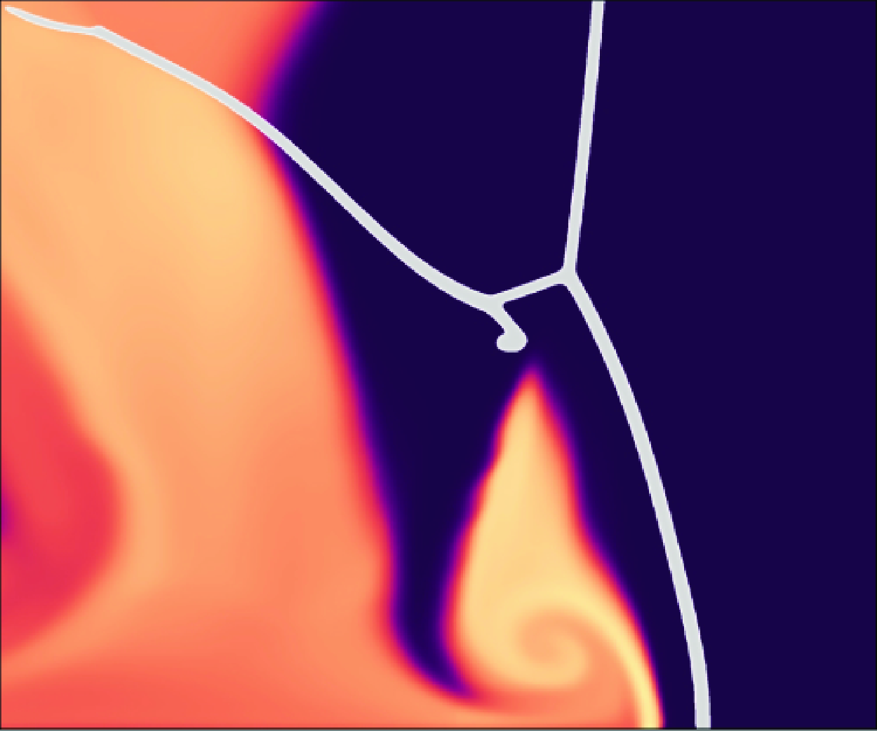
To clearly demonstrate the entire process of transverse wave creation in the detonation, the temperature and pressure gradient distributions in the detonation flow field (at six different times consisting of the purple lines in figure 5$a$) within a channel of $W = 3.5\,\rm mm$ filled with stoichiometric H$_2$/air are presented in figure 6. At $t = 93.6$ $\unicode {x03BC}\rm s$, there is only one triple point, TP1, on the front, where the transverse wave (see TW1 in figure 6) has begun to propagate from the upper wall towards the lower wall after reflection. During the collision of the transverse wave with the upper wall, a local explosion occurs, and thus induces a local overdriven detonation in the vicinity of the unreacted gas pocket, resulting in the formation of two forward explosion waves (FEWs) and two backward explosion waves. As time progresses to $t = 94.2$ $\unicode {x03BC}\rm s$, two FEWs gradually approach each other and subsequently merge into a single FEW. Due to the flow velocity and the acoustic impedance (or temperature) being uneven behind the Mach front, only part of the FEW passes through the reaction surface and approaches the Mach front at $t = 94.8$ $\unicode {x03BC}\rm s$. Next, the interaction of the FEW with the Mach front produces a kink marked by k1 on the Mach front at $t = 95.4$ $\unicode {x03BC}\rm s$. This interaction strengthens the Mach front above k1, which in turn increases the temperature of fluid behind the front. Since the stoichiometric H$_2$/air mixture is quite sensitive to temperature, the increase in flow field temperature induces a bulge flame on the reaction surface, as shown in the flow field at $t = 96.2$ $\unicode {x03BC}\rm s$. The flame accelerates and subsequently generates a compression wave (CW). This CW interacts with the detonation front to create a kink k2, which continues to propagate toward the lower wall. After the interaction between k2 and TP1, k2 passes through TP1, evolves into a new triple point TP2 and induces the transverse wave TW2. Ultimately, there are two triple points, TP1 and TP2, on the detonation front in the flow field, and the MLE fails.

Figure 6. The temperature and pressure gradient distributions of the detonation flow field at different times in the channel of $W = 3.5\,\rm mm$ filled with stoichiometric H$_2$/air mixture. The orange lines represent reaction surfaces of $Y(\mathrm {O}_2) = 0.118$: FEW – forward explosion wave, BEW – backward explosion wave, TW – transverse wave, CW – compression wave, TP – triple point, M – Mach front and I – incident front.

In essence, the creation of a new full developed TP undergoes in three stages. First, a FEW interacts with the Mach front, altering the strength of the Mach front. Second, a local bulge flame develops on the reaction surface due to the change in strength of the Mach front. Third, the bulging flame accelerates and induces a CW, which then interacts with the detonation front to form a new TP. The underlying cause of this sequence is a localized overdriven detonation at a spot with unreacted gases, triggered by a localized explosion. The effect of unreacted gas has also been mentioned in 1-D detonation studies (Sharpe & Falle Reference Sharpe and Falle2000; Daimon & Matsuo Reference Daimon and Matsuo2007). The explosion wave generated in an unreacted gas pocket can strengthen the 1-D detonation front, so as to maintain its propagation. However, the study of the impact of this explosion wave on multi-dimensional detonation fronts is still relatively limited. This paper presents a novel mechanism of generation of transverse waves that has not been fully explained before.

Figure 7. The temperature and pressure gradient distributions of the detonation flow field at different times in the channel of $W = 3.8\,\rm mm$ with stoichiometric H$_2$/O$_2$ mixture. The orange lines represent reaction surfaces of $Y(\mathrm {O}_2) = 0.4$: k – kink, TW – transverse wave, CW – compression wave, TP – triple point, WTP – weak triple point, M – Mach front and I – incident front.

Similarly, figure 7 displays the temperature and pressure gradient distributions in the detonation flow field within a channel of $W = 3.8\,\rm mm$ for a stoichiometric H$_2$/O$_2$ mixture, at twelve different times consisting of the purple lines in figure 5($b$). At $t = 29$ $\unicode {x03BC}\rm s$ after the collision between TP1 and the upper wall, the transverse wave reflects off the upper wall and propagates towards the lower wall. During the collision process, a forward jet is induced. This jet, with its strong impact force, interacts directly with the Mach front, causing the Mach front to bend at a point marked as k1. In a previous study (Mach & Radulescu Reference Mach and Radulescu2011), the aforementioned process is referred to as Mach reflection bifurcation (belonging to hydrodynamic instability). As time progresses, k1 gradually evolves into a distinct TP. Since the transverse wave induced by this TP has not yet fully developed, it is referred to as a WTP (see the WTP1 in the flow field at $t = 29.8$ $\unicode {x03BC}\rm s$). As shown in the flow fields at $t = 30.6$ $\unicode {x03BC}\rm s$ and 31.6 $\unicode {x03BC}\rm s$, the wave system around WTP1 interacts with the reaction surface, causing it to become unstable. This instability makes the formation of a series of CWs, which subsequently interact with the detonation front, resulting in the generation of WTP2 and WTP3.

During their downward propagation, WTP1 and WTP2 interact with TP1, which propagates upward after reflection on the lower wall; WTP1 and WTP2 pass through TP1. This interaction strengthens WTP1 and WTP2. Simultaneously, the increase in temperature behind WTP1 and WTP2 makes the fluid particles in their vicinity more reactive, which in turn benefits the sustenance of WTP1 and WTP2. At $t = 31.6$ $\unicode {x03BC}\rm s$, k2 is also generated by the interaction of the forward jet with the detonation front. When the time reaches $t = 32.2$ $\unicode {x03BC}\rm s$, WTP1 and WTP2 and k2 coalesce to form WTP4. Simultaneously, WTP3 interacts with TP1 and passes through it, leading to an enhancement of WTP3. Also, WTP4 reflects off the lower wall and moves towards WTP3, as shown in the pressure gradient distribution at $t = 32.8$ $\unicode {x03BC}\rm s$. Until $t = 33.6$ $\unicode {x03BC}\rm s$, the downward-propagating WTP3 and the upward-propagating WTP4 interact and penetrate each other. This interaction leads to an increase in the local fluid temperature, which in turn gives rise to a bulging of the reaction surface. Additionally, TP1 reflects off the upper wall and propagates downward, the k3 also appears after the action of a forward jet.

For the flow field at $t = 34.2$ $\unicode {x03BC}\rm s$, WTP4 interacts with TP1 and passes through it, and WTP4 is further strengthened. At this time, k3 evolves into a weaker WTP5, while WTP3 reflects off the lower wall and propagates upward. As time proceeds, WTP4 continues to propagate upward, while WTP5 gradually weakens and eventually dissipates due to interactions among the wave systems. At $t = 35.0$ $\unicode {x03BC}\rm s$, WTP3 just interacts with TP1, and they pass through each other, further strengthening WTP3. By $t = 35.6$ $\unicode {x03BC}\rm s$, WTP3 maintains its propagation upward, coincidentally as TP1 just reflects off the lower wall and also moves upward. After colliding with the upper wall, WTP4 travels towards WTP3. At $t = 36.4$ $\unicode {x03BC}\rm s$ after WTP3 and WTP4 interact, the fluid around them collides, creating an obvious high-temperature and high-pressure (HT and HP) region. Thus, this causes WTP3 and WTP4 to pass through each other, and the fluids of the HT and HP region propel WTP3 and WTP4 to propagate upward and downward, respectively. Lastly, WTP4 passes through TP1, and the transverse wave induced by WTP4 fully develops into TW2, thereby transforming WTP4 into TP2. Meanwhile, the upward-propagating TP1 engulfs WTP3. Consequently, there are now two TPs, TP1 and TP2, on the entire detonation front, indicating the failure of the MLE.

In summary, in the scenario of detonation in the channel filled with a stoichiometric H$_2$/O$_2$ mixture, the primary reason for the generation of a new fully developed transverse wave is the Mach reflection bifurcation. As mentioned earlier and in previous works (Semenov, Berezkina & Krassovskaya Reference Semenov, Berezkina and Krassovskaya2012; Shi et al. Reference Shi, Zhu, Yang and Luo2019), this bifurcation is caused by the forward jet, which is a manifestation of the flow non-uniformity within the flow field. Previous studies (Mach & Radulescu Reference Mach and Radulescu2011; Lau-Chapdelaine, Xiao & Radulescu Reference Lau-Chapdelaine, Xiao and Radulescu2021; Sow, Lau-Chapdelaine & Radulescu Reference Sow, Lau-Chapdelaine and Radulescu2021) have primarily relied on single-step global reaction models to investigate this process. However, the present paper is the first to thoroughly explore the generation of TPs caused by Mach reflection bifurcation based on real reactive system. Despite the use of different models, there is considerable qualitative consistency among them. Detailed analyses in this paper helps to deepen the understanding of the complex dynamics and interactions of detonation waves.

Notably, both failure mechanisms occur due to inherent instabilities within the detonation process. For detonations in stoichiometric H$_2$/air mixtures, the greater intrinsic chemical instability (higher effective activation energy) makes unreacted gas pockets more prone to forming localized explosion waves, leading to the failure of the MLE. In contrast, for detonations in stoichiometric H$_2$/O$_2$ mixtures, the stronger intrinsic flow instability (evidenced by higher detonation Mach numbers) causes bifurcations in the Mach front during Mach reflection, resulting in a failure of the MLE. For the failure mechanism of the MLE in H$_2$/air detonations, the interaction between explosion waves and the detonation front as a mechanism for cell growth is emphasized, which is not considered in previous studies.

3.3. Influence of channel width on mode locking

The above subsection indicates that the failure mechanisms of MLE for the two mixtures are distinctly different. This is consistent with the differences in channel width for the critical modes mentioned earlier, which are attributed to differences in the effective activation energies of the mixtures (i.e. their different temperature sensitivities). Although the MLEs fail in different ways for both mixtures, the failure is caused by changes in the channel width. However, it is not clear what influence the variation in channel width has on propagation of detonation waves, in other words, why would variation in channel width cause the MLE to fail?

Figure 8. Dimensionless longitudinal speed of detonation wave front as a time function on lower wall of $W$ = ($a$) 1.0 mm, ($b$) 1.5 mm and ($c$) 2.5 mm filled with a stoichiometric H$_2$/air mixture, and $W$ = ($d$) 1.0 mm, ($e$) 2.5 mm and ($f$) 3.5 mm filled with stoichiometric H$_2$/O$_2$ mixture. The dashed line indicates the CJ detonation speed.

To address the question mentioned above, here, we focus on the effects of channel width on detonation waves under the MLE, specifically in a single-headed mode. Figure 8 presents the variation over time of the longitudinal speed of the single-headed detonation wave fronts on the lower wall of the channel for different channel widths. Clearly, all the front speed curves exhibit highly periodic oscillation characteristics with period $T_{{d}}$. Nevertheless, the average speed of the detonation wave front primarily tends towards the theoretical CJ speed.

There are many jump features on the curves of figure 8, where the remarkable jump features are all generated by the collision of the front’s TPs on the lower wall. In figure 8($a$) with $W=1.0\,\rm mm$, the collision causes the detonation front speed to jump from approximately $0.85 D_{{CJ}}$ to approximately $1.25 D_{{CJ}}$, with a step magnitude of $0.40 D_{{CJ}}$. In the channel width of $W = 1.5\,\rm mm$, there is a jump from $0.80 D_{{CJ}}$ to $1.35 D_{{CJ}}$ shown in figure 8($b$), with a step magnitude of $0.55 D_{{CJ}}$, and the step magnitude has become larger. As the channel width further increases, the average step magnitude exceeds $0.6 D_{{CJ}}$, further suggesting the influence of channel width. Likewise, for the detonation of stoichiometric H$_2$/O$_2$ mixture, increasing the channel width also increases the step magnitude. For example, in figure 8($d$) with $W = 1.0\,\rm mm$, the magnitude is approximately $0.40 D_{{CJ}}$, while in figure 8($e,\!f$) with $W = 2.5\,\rm mm$ and 3.5 mm, the magnitudes are roughly $0.65 D_{{CJ}}$ and $0.80 D_{{CJ}}$, respectively. Potentially, the increase in instantaneous strength contributes to the failure mechanism of the MLE described earlier.

In fact, the period $T_{{d}}$ in figure 8 represents the time interval at which TP acts between on both walls under a single-headed detonation mode. In view of this, figure 9 presents the curve of the period $T_{{d}}$ along with variation of channel width. It can be seen that the period $T_{{d}}$ increases approximately linearly with the channel width. This period also reflects the duration of the Mach front of the detonation wave. Since fluid particles behind the Mach front are more likely to react, a longer-life Mach front promotes the formation of new fully developed TPs.

Figure 9. Period of interaction between the TP and the wall $dd^{\prime }$.

On the other hand, since transverse waves or TPs traverse a distance of double channel widths in one period, the average transverse wave speed $\overline {D}_{Z}$ (laboratory frame) can be obtained through $2W/T_{{d}}$. This average speed represents the motion characteristics of transverse waves in transverse space. To understand the impact of channel width on the motion of transverse waves, the diagrams of the average transverse speed of transverse waves versus channel width in a single-headed detonation scenario for both mixtures are shown in figure 10($a,\!b$). One can see from figure 10 that the average transverse speed of the TPs increases as the channel width increases for both mixtures. This implies that the transverse motion of the transverse wave in the detonation becomes stronger for a wider channel. Since the explosion wave and Mach reflection, as described earlier, both originate from the collision of the transverse wave on the wall, stronger transverse motion of transverse wave structures is necessary to trigger strong explosion waves or Mach reflection.

Figure 10. Average transverse speed of TP under ($a$) stoichiometric H$_2$/air and ($b$) stoichiometric H$_2$/O$_2$ mixtures as functions of channel widths. Here, $D_{{CJ,i}}$ and $a_{{i}}$ are the CJ detonation speed and the speed of sound in the induction zone, respectively, calculated based on the post-shock states of the 1-D steady-state CJ-ZND structure.

To summarize, increasing the channel width not only intensifies the explosion waves and Mach reflections arising from the collision of transverse wave on the wall but also extends the time interval between two collisions. These changes make the reaction surface more susceptible to destabilization and allow more time for the destabilized reaction surface to develop, thus causing the MLE to fail ultimately. On the other hand, when the channel width is too small, transverse wave structures cannot exist continuously; that is, TPs appear intermittently (see figure 3$a{,}e$) or do not appear at all (see the work of Chinnayya, Hadjadj & Ngomo Reference Chinnayya, Hadjadj and Ngomo2013). According to figure 10, it can be inferred that, under extremely small channel width conditions, the transverse wave structure with an average transverse speed slightly greater than or close to the induction zone’s sound speed is not allowed to constantly exist within the flow field, thereby the failure of the MLE is caused by a different way. The specific reasons are discussed in subsequent sections.

3.4. Details of transverse wave structure

The detonation modes described in the above sections are closely related to transverse wave (TW) structure. Particularly, the appearance and transverse motions of the TW structure affect the MLE. Therefore, it is necessary to deepen study the TW structure of the detonation.

Figure 11. Shock waves indicated by high pressure gradient and reaction surfaces given by the isoline of $Y$(O$_2$) = 0.118 (left) or $Y$(O$_2$) = 0.4 (right) in the channel of $W$ = ($a$) 1.0 mm, ($b$) 2.5 mm and ($c$) 4.0 mm with stoichiometric H$_2$/air mixture, and $W$ = ($d$) 1.0 mm, ($e$) 3.5 mm and ($f$) 4.0 mm with stoichiometric H$_2$/O$_2$ mixture. For each snapshot, its height represents the full channel width, and the aspect ratio in both horizontal and vertical directions is 1:1.

Figure 11 displays the shock structures and reaction surfaces for different mixtures at different channel widths, represented by pressure gradient distributions overlapped by contours of species O$_2$. Clearly, the TW structures in detonations studied in this paper all belong to STW structures, which are characterized by the presence of two TPs, designated as A and B, near the detonation front. This structure is consistent with the schematic shown in figure 1, illustrating the ubiquity of STW structures. When conditions are near the threshold of the critical propagation state, at 48.10 $\unicode {x03BC}$s and 49.15 $\unicode {x03BC}$s displayed in figure 11($a$), a distinct unreacted gas groove is present near the STW structures in the flow field, indicating that the STW structures under this condition are of the second kind defined as figure 1($b$). As the channel width increases, the structure of the TWs is affected. It can be seen that there are differences in the flow field near the strong structures in figure 11($b$). At 105.20 $\unicode {x03BC}$s, a pronounced groove is present in the flow field, indicating that the TW structure at this time is of the second kind of STW structure. While at 107.60 $\unicode {x03BC}$s, a TD wave completely replaces the groove, transforming the TW structure into a first kind of STW structure. This significant difference is primarily due to the fact that stoichiometric H$_2$/air mixtures are relatively unstable. However, as shown in figure 10($a$), the average transverse speed of the TWs under the condition of figure 11($b$) is much lower than the CJ detonation speed, so it can be inferred that the occurrence of such TD that exits in the first kind of STW structure is relatively difficult in 2-D detonation. As a result, the TW structure is mainly dominated by the second kind of STW structure. When the detonation propagates in the wider channel shown in figure 11($c$), there are two STW structures (indicated by TPs A$_1$ and A$_2$) in the flow field, with unreacted grooves around them. This again indicates that the second kind of STW structure is a more fundamental feature of 2-D detonations.

For a stoichiometric H$_2$/O$_2$ mixture, the TW structure of the detonation wave propagating when conditions approach the threshold of the critical propagation state also features the second kind of STW structure with unreacted gas grooves, as shown in figure 11($d{-}\!f$). For such a relatively stable mixture, as the channel width increases, the unreacted groove region becomes small. However, even though the groove area has decreased, the transverse average speed of the structure (approximately $0.6 D_{{CJ}}$) shown in figure 10($b$) is significantly lower than the CJ detonation speed, indicating that TD is difficult to occur. This means that the entire TW structure still falls under the category of the second kind of STW structure. Furthermore, for the dual-headed mode of the H$_2$/O$_2$ mixture shown in figure 11($f$), the TWs also clearly show the second kind of STW structures. Totally, the second kind of STW structure plays a predominant role in the 2-D detonations of the present work.

To further observe the relationship between the transverse motion and the flow field structure, figure 12 presents the variation over time in the transverse instantaneous speeds $\left | D_{Z} \right |$ of the TPs under a single-headed detonation mode. In one period, there are two stages in which the transverse speed gradually increases to cross $a_{{i}}$ for all curves in figure 12, where the TP of first stage is from the lower wall to the upper wall, and the TP of second stage is from the upper wall to the lower wall. For the H$_2$/air detonation at $W = 1.0\,\rm mm$ (figure 12$a$), the instantaneous transverse speed of the TP is overall much smaller than the CJ detonation speed, which implies that the TD is unlikely to appear in the flow field. As can be seen from figure 11($a$), there exists a significant unreacted groove in the flow field without the presence of the TD, indicating that the flow field is dominated by the typical second kind of STW structure. For the detonation of such unstable gases as H$_2$/air mixtures, a wider channel allows more space and time for the development of detonation instability. Under the influence of this instability, the transverse speed exhibits chaotic characteristics, accompanied by abrupt acceleration in transverse speed, as illustrated in figure 12($b$). This abrupt change in transverse speed can cause the speed value to approach the CJ detonation speed, thus enabling the development of TD in the flow field. However, from a statistical perspective (see figure 10$a$), the average transverse speed of the TP is significantly lower than the CJ detonation speed, which means that such sudden accelerations and the subsequent appearance of TDs are relatively rare, thus the flow field predominated by the second kind of STW structure is considered.

Figure 12. Transverse instantaneous speeds of the TPs as a function of time in the channel of $W$ = ($a$) 1.0 mm and ($b$) 2.5 mm filled with stoichiometric H$_2$/air mixture, and $W$ = ($c$) 1.0 mm and ($d$) 3.5 mm filled with stoichiometric H$_2$/O$_2$ mixture. Here, $D_{{CJ,i}}$ and $a_{{i}}$ are the CJ detonation speed and the speed of sound in the induction zone, respectively, calculated based on the post-shock states of the 1-D steady-state CJ-ZND structure.

Similarly, when the channel width is relatively small, the transverse speed of the TP in a single-headed H$_2$/O$_2$ detonation is also much lower than the CJ detonation speed (see figure 12$c$), indicating that the TW intensity is weaker and the flow field exhibits the typical second kind of STW structure shown in figure 11($d$). Particularly, for the wider channel of figure 12($d$), due to the relative stability of the detonation in this mixture, the transverse speeds in both the first and second stages increase overall more smoothly. Compared with H₂/air detonations, this trend is more orderly. It can be seen that widening the channel results in an overall increase in the transverse speed of the TP in a single-headed H$_2$/O$_2$ detonation. Correspondingly, under the condition of figure 11($d$), the unreacted groove is smaller but observable. Hence, the TW structure of the flow field is considered to be a second kind of STW structure. However, the quantitative relationship between the transverse speed and the size of the groove is currently unknown, thus necessitating theoretical analysis.

The above results indicate that the second kind of STW structure is more important and prevalent in 2-D detonations for both H$_2$/O$_2$ and H$_2$/air mixtures. It is noted that, as the channel width decreases, the maximum instantaneous transverse speed (as shown in figure 12) of the TP is reduced. It is evident that, in extremely narrow channels, the transverse speed of the TW near the wall cannot increase to a sufficient value, which prevents the maintenance of the STW structure and leads to the failure of the MLE. The factors for maintaining the STW structure are quantitatively analysed in § 4.

When the TWs approach the situation of TP disappearance (i.e. under $W = 1.0\,\rm mm$), the average transverse speed of the STW structure is very close to $a_{{i}}$, as shown in figure 10. Actually, a typical second kind of STW structure that just meets the speed of sound condition exhibits an acoustic coupling characteristic. To further recognize this acoustic coupling characteristic of the structure, figure 13 shows the wave structures of different times and the numerical foil of vorticity in the 2-D domain of $W = 1.0\,\rm mm$ with two mixtures. Obviously, during the upward movement of the TP, the TW structure is consistently “strong” type (Mahmoudi & Mazaheri Reference Mahmoudi and Mazaheri2015), moreover corroborating the importance of the STW structure. The black slim lines composed of higher vorticity on the foil of vorticity accurately indicate the movement trajectory of the TP A on the detonation front since the value of vorticity around A is larger. When the slim line segment appears like a left slash, as with segment $lm$, it represents the TP moving from bottom to top; otherwise, the TP moves in the opposite direction. The trajectory of the acoustic wave, indicated by the black dashed lines in figure 13, closely coincides with the trajectory of the TP for the two mixtures. This further demonstrates that a typical second kind of STW structure exhibits acoustic coupling characteristics. It is noteworthy that the aforementioned acoustic coupling characteristic in 2-D detonation is unusual, as previous literature (Fay Reference Fay1952; Sugiyama & Matsuo Reference Sugiyama and Matsuo2013) has primarily addressed acoustic coupling in the context of a typical first kind of STW structure.

Figure 13. Numerical foils of vorticity and wave structures near detonation front in the 2-D domain of $W$ = 1.0 mm filled with ($a$) stoichiometric H$_2$/air and ($b$) stoichiometric H$_2$/O$_2$ mixtures. The vorticity $|\omega |$ is calculated using $|\boldsymbol {\nabla }\times (\boldsymbol {U})|D_{{ref}}/D_{{CJ}}$, where $D_{{ref}}$ is the reference speed, which is set to 2000 m/s in this paper. The black dashed line indicates the trajectory of an acoustic wave in the induction zone of CJ-ZND structure.

4.1. Prediction of the high-pressure value

To conduct shock polar calculations, one first needs to know the transverse speed $D_Z$, the longitudinal speed $D_X$ of TP A and the angle $\chi _{ {I}}$, as shown in figure 15. For the purpose of usability and generality, it is necessary to establish a reasonable assumption for the basic parameters used in calculating the shock polar. This strategy allow us to theoretically derive a reasonable physical quantity for the apparent transverse dynamics of detonation.

The selection of appropriate assumptions is crucial. At the outset, we can only rely on intuitive statistical averages to hypothesize about the research object. Therefore, for the typical second kind of STW structure of single-headed detonation in a 2-D channel, several assumptions can be made as follows:

1. (i) Since acoustic coupling occurs between the typical second kind of STW and the acoustic wave in the induction zone of the CJ-ZND structure (see § 3.4), $D_Z$ in equation (4.1) is assumed as $a_{{i}}$.

2. (ii) The CJ detonation is considered here (see result of figure 8), so $D_X$ in equation (4.1) is determined as $D_{{CJ}}$.

3. (iii) It is assumed that the angle $\chi _{{M}}$ ranges from $90^\circ$ at maximum to $90^\circ - \alpha$ at minimum. The linear changes on space or time are considered for $\chi _{{M}}$, thus the Mach front’s average angle is $\chi _{{M,avg}} = (\chi _{{M,min}} + \chi _{{M,max}})/2 = 90^\circ - 0.5\alpha$. For a 2-D single-headed detonation, since the Mach front transforms into an incident front after the STW structure collides with the wall, the angle $\chi _{ {I}}$ is construed as

   (4.3) \begin{align} \chi _{ {I}} = \chi _{{M,avg}} = 90^\circ - 0.5 \arctan (a_{{i}}/D_{{CJ}}) . \end{align}

Based on the aforementioned assumptions, the incoming flow velocity relative to the TP A is here determined using $V_{ {(0)}} = D_{{CJ}}/\cos (\alpha )$, and the angle $\beta$ of incident front can be determined by $\beta = \chi _{ {I}} - \alpha$. The assumed value of $\theta _{(1)}$ and other flow states behind the incident front can be obtained by substituting the assumed values of $\beta$ and $V_{ {(0)}}$ into the shock jump condition using the iterative method mentioned in Appendix C. Figure 17 displays the shock polars for the second kind of STW structure with a stoichiometric H$_2$/air mixture. Eventually, the pressure value and deflection angle $\theta _{(4),(5)}$ of the states (4) and (5) in the HP region of the STW can be determined by the red point in figure 17($a$).

Figure 17. The polars of ($a$) pressure ratio and ($b$) wave angle with a stoichiometric H$_2$/air mixture. The numbers in parentheses represent the flow states and wave angles in the corresponding flow regions. The extended segments are the strong shock part of the shock polar with a wave angle larger than $90^\circ$.

Moreover, the wave angle $\beta$ for different shock waves in the STW can also be derived by utilizing the deflection angle $\theta _{(i)}$ of different states and the polar represented in figure 17($b$). These parameters enable us to construct a shock wave pattern that closely resembles the shock wave system of STW structure, as shown in figure 15. The extended segments on the blue and green polar are depicted in figure 17, illustrating the potential state behind the secondary Mach stem and the secondary reflection shock wave. On the one hand, for a Mach reflection in free space, the Mach stem can either increase (extended segment on blue polar) or decrease the deflection angle, e.g. the overall Mach reflection of asymmetric shock waves (Ben-Dor Reference Ben-Dor2007). On the other hand, for the secondary reflection shock wave, a shock system that is similar to the von Neumann reflection is considered, which means the states (4) and (5) in some situations can be given by the intersection point between the blue polar and the extended segment of the green polar. One can note that this paper stipulates that the Mach stems (M and line segment BD in figure 15) only exist when the solution corresponds to a strong shock wave.

To verify the accuracy of the prediction of polar presented in this paper, figure 18 displays the pressure ratio $p/p_0$ changes over time in the HP region of the second kind of STW structure for both mixture cases, by using numerical simulation and shock polar. At each moment, the HP value for the numerical simulations is determined by averaging the numerical values from three to five grids. These grids are positioned approximately two grid points downstream of point B and its adjacent shock waves. Here, the given time range for figure 18 corresponds to the stage at which the TW propagates upward from the lower wall to the upper wall for both mixtures, as shown in figure 13. It can be observed from figure 18 that, in the early phases, the pressure values from the numerical results align well with the ideal value, indicating the effectiveness of the theoretical method in this paper and the reasonability of the assumptions made above.

Figure 18. The pressure ratio given by the shock polar and numerical result with ($a$) stoichiometric H$_2$/air and ($b$) stoichiometric H$_2$/O$_2$ mixtures. Dashed-dotted lines represent the values determined by shock polar. Ideal value: the value calculated based on assumptions in this sub-section, final and lowest limit values: the values calculated based on the evolution behaviour of the STW structure discussed in the next sub-section.

Since the assumptions for the polar do not account for the temporal dynamics of the second kind of STW structure, the ideal values (indicated by the red dash-dot lines in figure 18), determined by the shock polar based on the assumptions in this section, remain constant over time. However, the numerical data indicate that the pressure in the HP region does not remain steady but decays over time. When the STW approaches the wall, there is a substantial discrepancy between the ideal values and the numerical results. This difference is analysed in the following sub-subsection.

4.2. Transverse dynamic behaviours

To explore the impact of time-dependent behaviours of the STW structure on the pressure values of states (4) and (5), several key influencing factors are sought here through the shock polar method combined with the numerical results of the 2-D detonation described in previous sections. Firstly, one notes that angle $\chi _{ {I}}$ can continuously increases to $90^\circ$ by observing figure 13. However, the influence of the change of $\chi _{ {I}}$ on the flow states around STW is still unclear.

To understand the influence of the angle $\chi _{ {I}}$ on the HP value of states (4) and (5), figure 19 presents a set of $(p/p_0, \theta )$ polar as the angle $\chi _{ {I}}$ varies, while the track angle $\alpha$ of TP A is still determined by the assumptions in § 4.1. The results show that, as $\chi _{ {I}}$ changes, the predicted pressure values of the states (4) and (5) form a trajectory marked in the black curve in figure 19. The evolution of the pressure value along this curve suggests that an increase in the incident front angle $\chi _{ {I}}$ leads to a decrease in the pressure value of states (4) and (5), which is due to a reduction in the total flow Mach number of state (1). This pressure change coincides precisely with the described pressure decay characteristics in figure 18, thus the angle $\chi _{ {I}}$ is considered as a key factor influencing the pressure of states (4) and (5). Interestingly, as shown in figure 19, when $\chi _{ {I}}$ is $82^\circ$ or $84^\circ$, the states (4) and (5) cannot be given by the polar, which means the von Neumann criterion (Ben-Dor Reference Ben-Dor2007; Peng et al. Reference Peng, Zhang, Hu and Jiang2019) is not reached, indicating that the flow intensity of state (1) cannot form a secondary Mach reflection for larger $\chi _{ {I}}$. However, the numerical results of wave structures in figure 13 suggest that, even when $\chi _{ {I}}$ tends very close to $90^\circ$, the TW still manifests as an STW structure, implying that the states (4) and (5) may simultaneously depend on other controlling factors besides $\chi _{ {I}}$.

Figure 19. The ($p/p_0$, $\theta$) polars at different $\chi _{ {I}}$ with a stoichiometric H$_2$/air mixture.

Recall that, in assumption (ii) of § 4.1, the longitudinal speed $D_X$ is set to a constant value ($D_{{CJ}}$). Actually, before TP A contacts the wall, $D_X$ should be close to the incident front speed $D$ due to the incident front being nearly perpendicular to the wall, as shown by the wave structure of $t = 48.40$ $\unicode {x03BC}\rm s$ in figure 13($a$) and $t = 46.40$ $\unicode {x03BC}\rm s$ in figure 13($b$). When TP A is about to interact with the wall $dd^{\prime }$, $D_X$ equals $D$ and is less than $D_{{CJ}}$, and the transient deviation between $D_X$ and $D_{{CJ}}$ can reach up to 20%, as indicated by figure 8. Thus, the assumption that $D_X = D_{{CJ}}$ may lead to a discrepancy between the predicted values and actual ones.

To explore the influence of $D_X$ on the pressure of states (4) and (5) in the HP region, $D_Z$ is fixed as $a_{ {i}}$, and the pressure changes for states (4) and (5) under different $\chi _{ {I}}$ and $D_X$ are depicted in figure 20. The decrease in $D_X$ leads to an overall weakening of the STW structure, resulting in a reduction in the pressure values of states (4) and (5), as shown in figure 20. Therefore, $D_X$ can also be considered a key factor for the decay of pressure in the HP region. Furthermore, with the longitudinal speed $D_X$ decrease, the upper limit of incident front angles has increased from $81^\circ$ at $D_X = D_{{CJ}}$ to $84^\circ$ at $D_X = 0.85D_{{CJ}}$, and the range of incident front angles has expanded, as demonstrated by figure 20. This expansion is attributed to the decreased incoming flow Mach number in the $\xi$-direction (the decreased incident front strength), which indirectly results in the elevated transverse ($\eta$-direction) flow Mach number downstream of the incident front. Eventually, this adjustment provides ample flow intensity in region (1), facilitating the formation of secondary Mach reflection.

Figure 20. Dimensionless pressure of states (4) and (5) as a function of the angle $\chi _{ {I}}$ and the longitudinal speed $D_X$ of TP A with a stoichiometric H$_2$/air mixture and $D_Z = a_{ {i}}$.

On the other hand, combining the results of the present and previous works (Radulescu et al. Reference Radulescu, Sharpe, Law and Lee2007; Liang et al. Reference Liang, Browne, Deiterding and Shepherd2007; Frederick et al. Reference Frederick, Gejji, Shepherd and Slabaugh2023), it can be concluded that there exists a minimum $D_X$ for the self-sustained 2-D detonation, which is approximately $0.85D_{{CJ}}$ for the typical second kind of STW structure as shown in figure 8($a,\!d$) in the present study. Although the reduction in $D_X$ broadens the range of $\chi _{ {I}}$, as shown in figure 20, the upper limit of $\chi _{ {I}}$ always remains well below 90 degrees, indicating that there are still other parameters controlling the TW structure and flow state. It is observed in figure 12 that the transverse speed $D_Z$ of TP A exceeds $a_{ {i}}$ for a long time, but $D_Z$ is assumed as the sound speed $a_{ {i}}$ in the induction zone of the CJ-ZND structure. For this reason, the focus now shifts to the effects of the potential last parameter, $D_Z$.

Figure 21 depicts the variation of pressure with respect to $\chi _{ {I}}$ and $D_Z$, where $D_X$ is maintained at the minimum value $0.85D_{{CJ}}$. Indeed, the increase in $D_Z$ leads to a rise in the pressure value of the HP region, which is attributed to the strengthening of the entire STW structure during the increase in the transverse speed. Increasing the transverse speed at the TP directly raises the transverse flow Mach number in region (1) relative to point A. This facilitates adequate flow intensity for forming a secondary Mach reflection structure. Therefore, even when $\chi _{ {I}}$ equals 90 degrees, the TW structure remains a strong type.

Figure 21. Dimensionless pressure of states (4) and (5) as a function of the angle $\chi _{ {I}}$ and the transverse speed $D_Z$ of TP A with a stoichiometric H$_2$/air mixture and $D_X = 0.85D_{{CJ}}$.

In summary, two key factors dominate the pressure decay in the HP region: the incident front angle $\chi _{ {I}}$ and the speed $D_X$. Under the influence of both factors, there is a theoretical lowest limit for the pressure value of the states (4) and (5), as indicated by the black arrows in figures 20 and 21. This lowest limit is also marked in figure 18. On the other hand, the variations in the third factor, i.e. the transverse speed $D_Z$, cause an increase in the HP value of states (4) and (5). Since $\chi _{ {I}}, D_X,$ and $D_Z$ change concurrently, the pressure values derived from numerical simulations are disabled to reach this theoretical minimum. For the single-headed detonation investigated in the present study, due to theTW structure needing to remain an STW structure throughout, there exists a minimum value for the upper limit of $D_Z$. This ensures that, even when $\chi _{ {I}}$ is $90^\circ$ and $D_X$ is $0.85D_{{CJ}}$, the HP region persists. As depicted in figure 21, the dynamic change of the factors ultimately settles at the position (indicated by the blue arrow) where $\chi _{ {I}}$ equals 90 degrees, indicating the minimum value (approximately 1.25$a_{ {i}}$) for the upper limit of $D_Z$ and the pressure value of the HP region at the final situation. This final value is also plotted in figure 18 for comparison. It is evident that the three specific values obtained by shock polar effectively capture the features of the transverse structure dynamics.

Simultaneously, combining the discussions in this sub-section with those in §§ 3.3 and 3.4, it is evident that increasing the channel width results in a higher transverse speed of the TW structure, but has little effect on the longitudinal speed of the TP (with an average value of $D_{{CJ}}$ and a minimum value in the range of 0.80–0.85$D_{{CJ}}$, as shown in figures 8 and 10) and the angle of the incident front (the angle tends towards $90^\circ$, see figures 11 and 13). As a result, the increase in channel width primarily enhances the transverse strength of the STW structure. A wider channel induces stronger collisions between the STW and the wall, which facilitates the formation of new TPs and leads to the failure of the MLE. Conversely, a narrower tube prevents the STW structure from meeting the minimum upper limit condition of the transverse speed, causing the STW structure to be unsustainable and leading to the failure of the MLE as well.

4.3. Quantitative identification on strong transverse wave

In the discussion of the § 3.4, the classification of STW structures is primarily based on observation, which is somewhat subjective and qualitative. Therefore, identifying the quantitative difference between the two typical kinds of STW structures is of primary significance. The constant-volume combustion (CVC) theory is widely used for the calculation of ignition times in shock-induced combustion, such as predicting the induction zone length in oblique detonations (Zhang et al. Reference Zhang, Liu and Yan2019b) and the strong ignition time (Huang et al. Reference Huang, Wang, Deiterding, Yu and Chen2022). To quantitatively identify the structure of the STW, the reaction spatial scale calculations downstream of TP B based on CVC theory are performed in this section.

For spatial-coordinate-based CVC computation, a determination of the temperature and total flow velocity conditions near the STW is necessary. As a result, figure 22 displays the temperature ratio and total flow velocity polars based on the shock polar method described in § 4.1. By integrating the pressure and temperature polars (see figures 17$a$ and 22$a$, respectively), and assuming that the mixture in region (4) near point B remains as an unburned mixture, the variation of temperature with combustion time $\tau _{{CVC}}$ can be determined using CVC theory. To characterize the spatial scale of the reaction zone near the STW, we define a transverse chemical reaction distance $\zeta _{{r}} = \tau _{{CVC}} V_{(4)}$, where $V_{(4)}$ is the total flow velocity of state (4), as shown in figure 22($b$).

Figure 22. The polars of ($a$) temperature ratio and ($b$) flow velocity with a stoichiometric H$_2$/air mixture. The numbers in parentheses represent the flow states in the corresponding flow regions.

Figure 23 shows the variation of dimensionless temperature $T/T_0$ with respect to dimensionless transverse reaction distance $\zeta _{{r}}/\Delta _{{ind}}$ ($\Delta _{{ind}}$ is the induction length from the 1-D CJ-ZND structure) for the typical second kind of STW with the stoichiometric H$_2$/air and H$_2$/O$_2$ mixtures of the current study. For the purpose of comparison, the temperature profiles of the typical first kind of STW with a stoichiometric H$_2$/air mixture observed in Tsuboi & Hayashi (Reference Tsuboi and Hayashi2007) and stoichiometric H$_2$/O$_2$ mixture observed in Tsuboi, Hayashi & Koshi (Reference Tsuboi, Hayashi and Koshi2009) are also calculated. For several CVC cases shown in figure 23, the initial parameters required for shock polar calculation used in CVC computations are listed in table 2. Among them, the initial parameters for the second kind of STW structure are given by the assumptions in § 4.1, while the initial parameters for the first kind of STW structure are derived from measurements of previous research (Tsuboi & Hayashi Reference Tsuboi and Hayashi2007; Tsuboi et al. Reference Tsuboi, Hayashi and Koshi2009).

Table 2. Calculation parameters of shock polar serving CVC computations.

Figure 23. Dimensionless temperature as a function of the dimensionless transverse chemical reaction distance with constant-volume combustion and the parameters of state (4). The red lines indicate the locations of ignition.

Based on figure 23, we can define an ignition delay distance $\zeta _{ {i}}$ as the distance from the start of the reaction (i.e. TP B) to the location of ignition and this is used to derive a quantitative index of reactivity. The values of $\zeta _{{i}}/\Delta _{{ind}}$ for different cases are indicated by the red lines in figure 23, where a rapid increase in temperature is observed. Obviously, due to the extremely short ignition delay distance $\zeta _{{i}}$ ($\zeta _{{i}}/\Delta _{{ind}} \ll 1$, indicated by red dash-dot and red dash-dot-dot lines in figure 23) downstream of TP B in the STW structure of Tsuboi & Hayashi (Reference Tsuboi and Hayashi2007) and Tsuboi et al. (Reference Tsuboi, Hayashi and Koshi2009), a TD is observed, rendering the entire STW structure of spinning detonation as the typical first kind of STW structure. On the contrary, a quite long ignition delay distance ($\zeta _{{i}}/\Delta _{{ind}} \to 1$) is required downstream of TP B of the TW structure in the present detonation, suggesting the presence of an unreacted groove containing premixed mixture. This characteristic is a typical feature of the second kind of STW structure described in this paper.

There is an order of magnitude difference in reactivity (i.e. ignition delay distance) between the typical two kinds of STW structures. The downstream ignition delay distance at the TP B of the typical second kind of STW structure is comparable to the induction zone length, which shows consistency with the results shown in figure 14. This further validates the assumptions proposed in § 4.1. Interestingly, as shown in table 2, the track angle of the typical first kind of STW structure always approaches $45^{\circ }$, whereas the track angle of the typical second kind of STW structure is closer to $24^{\circ }$. Here, the track angle actually corresponds to the average track angle of the TP. This indicates an important parameter for distinguishing the kinds of STW structures in detonations, namely, by measuring the average track angle (ATA, calculated by $\overline {\alpha } = \arctan (\lambda /\ell )$, where $\lambda$ and $\ell$ are the width and length of cell, respectively) of the TPs on the cell structure to assess the reactivity of the TW structure.

In § 3, the classification of STW structures is somewhat arbitrary, as all STW structures discussed are classified as the second kind, which is somewhat subjective. To provide a quantitative criterion for distinguishing both kinds of the STW structures for the purpose of engineering or experiments, figure 24 further illustrates the relationship between the ATA and $\zeta _{{i}}/\Delta _{{ind}}$ under different conditions, in which the angle $\chi _{ {I}}$ follows equation (4.3) for obtaining relevant shock polars. One can observe that the ATAs of detonation in the rectangular channel are smaller than the value of a median (as shown by the vertical dash-dot line in figure 24), and Austin (Reference Austin2003) also pointed out that the ATA in a rectangular channel is $33^\circ$ and is less than the median. Whereas the ATAs in the circular channel are all greater than the value of median. Therefore, this median is important for distinguishing or identifying the characteristics of confined spaces where TWs are located.

Figure 24. Relationship between the ATA and the $\zeta _{{i}}/\Delta _{{ind}}$ under different conditions. The square and circular markers represent the propagation of detonation waves in rectangular and circular channels, respectively. The black dash-dot line represents the median of the ATA for the two typical kinds of STW structures. $^{ {a}}$Meagher et al. (Reference Meagher, Shi, Santos, Muraleedharan, Crane, Poludnenko, Wang and Zhao2023), $^{ {b}}$Crane et al. (Reference Crane, Lipkowicz, Shi, Wlokas, Kempf and Wang2023), $^{ {c}}$Tsuboi et al. (Reference Tsuboi, Hayashi and Koshi2009) and $^{ {d}}\log (\zeta _{{i}}/\Delta _{{ind}}) = 1.041 - 0.057\overline {\alpha }$.

On the other hand, a logarithmic law between the ATA and the dimensionless ignition delay distance was observed after conducting a linear regression analysis (as indicated by the red dashed line in figure 24) for all of the data appearing in figure 24. Notably, the value of the point where the red dashed line intersects the horizontal line at $\zeta _{{i}}/\Delta _{{ind}} = 0.1$ is found to be very close to the median. Thus, this median, $\overline {\alpha } = 35^\circ$, that corresponds to $\zeta _{{i}}/\Delta _{{ind}} = 0.1$, is crucial as it reflects both the characteristics of the confined space and the reaction scale. Furthermore, given the ease of obtaining the ATA and its ability to represent the kinematic characteristics of STW structures, the distinction and classification of STW structures are ultimately realized by determining the value of the ATA. If the angle is greater than the median, the STW structure is classified as first kind; otherwise, it is classified as second kind.

As previously mentioned, the detonation in circular channels exhibits a significantly different TW structure (often characterized by the first kind of STW structure), which is due to the more complex interactions between the TWs and the circular channel walls, reflecting complex 3-D effects. This paper primarily focuses on 2-D detonations and cannot fully explain this phenomenon. Moreover, the detonations discussed in this study propagate in weakly unstable and moderately unstable mixtures. For highly unstable mixtures, complex interactions between shock waves and turbulence may occur within the detonation wave, and the applicability of the current theory requires further consideration. Accordingly, these two aspects will need to be addressed in future work.