


1. Introduction
Wall jets can be regarded as boundary-layer flows where the free-stream velocity  $U_\infty$ is exceeded at some near-wall location. Initiated by the introduction of momentum flux (eventually) directed along a solid surface, such flows are encountered in a variety of engineering applications, perhaps most prominently in those related to heat transfer. To cite only one example, the thermal load acting on gas turbine blades is typically reduced by external wall jets providing a shielding air film as well as radial wall jets caused by the impingement of air onto the internal blade surface. Extensive review articles addressing various wall jet configurations are provided by Launder & Rodi (Reference Launder and Rodi1979, Reference Launder and Rodi1983).
The major characteristics of steady, turbulent wall jets were arguably first addressed by Förthmann (Reference Förthmann1934), extending the work of Tollmien (Reference Tollmien1926) regarding a free shear layer to the wall-bounded configuration. More recent investigations address the complex nature of this flow that is governed by different types of coherent structures according to Gnanamanickam et al. (Reference Gnanamanickam, Bhatt, Artham and Zhang2019). Among those, forward-leaning flow structures have been revealed as the main source of an interaction between the inner and outer regions that are separated by the location of maximum streamwise velocity (Bhatt & Gnanamanickam Reference Bhatt and Gnanamanickam2020; Artham, Zhang & Gnanamanickam Reference Artham, Zhang and Gnanamanickam2021).
The presence of such intricate flow structures has rendered the identification of universal scaling laws a challenging task. Glauert (Reference Glauert1956) showed that the spreading rate of turbulent wall jets can be described satisfactorily by introducing the concept of an eddy viscosity. However, complete similarity is not attainable as this eddy viscosity evolves non-synchronously in the inner and outer layers of the wall jet. Nonetheless, ‘approximate self-similarity’, i.e. similar velocity profiles, when scaled with the maximum velocity  $U_m$ at respective streamwise locations and the jet outlet width
  $b$, was reported soon afterwards by Bakke (Reference Bakke1957) and Sigalla (Reference Sigalla1958). They also show that
  $U_m$ decays with a power law in the form
  $U_m\propto x^a$, where
  $a=-1/2$ for the case of a two-dimensional wall jet. Similar values of the power-law exponent have been stated by Bradshaw & Gee (Reference Bradshaw and Gee1962) and Myers, Schauer & Eustis (Reference Myers, Schauer and Eustis1963) whereas a significant deviation was found, for instance, by Schwarz & Cosart (Reference Schwarz and Cosart1961) where
  $a=-0.62$, suggesting an inadequacy of the conventional scaling quantities. Against this backdrop, Narasimha, Narayan & Parthasarathy (Reference Narasimha, Narayan and Parthasarathy1973) evaluated experimental datasets of plane wall jets ejected in still air available at the time and showed that near-outlet parameters, namely the jet velocity
  $U_j$ and the nozzle geometry, become irrelevant in the region of a ‘fully developed flow’, say at
  $x/b>30$. Instead, they argue that the ejected momentum flux
  $J$ and the kinematic viscosity
  $\nu$ should be used to determine the jet development. Specifically, these gross properties were shown to be suited to describe the decay of
  $U_m$ and wall shear stress
  $\tau$ as well as the expansion rate, which was later confirmed by Wygnanski, Katz & Horev (Reference Wygnanski, Katz and Horev1992) and George et al. (Reference George, Abrahamsson, Eriksson, Karlsson, Löfdahl and Wosnik2000). Recently, the approach suggested by Narasimha et al. (Reference Narasimha, Narayan and Parthasarathy1973) was taken up by Gupta et al. (Reference Gupta, Choudhary, Singh, Prabhakaran and Dixit2020) who propose the use of the local momentum flux instead of the jet momentum flux at the outlet, thus establishing robust scaling laws that are independent of initial conditions and therefore consistent with the notion of self-similarity. However, substantial additional effort is introduced because local velocity profiles are required. Thus, the approach suggested by Narasimha et al. (Reference Narasimha, Narayan and Parthasarathy1973) appears to be easier to adopt in technical applications and will therefore be pursued in the current study. Notably, this method is not limited to the case of wall jets emitted into still ambience but also applies when there is a steady, uniform co-flow as long as the excess in kinematic momentum flux is sufficiently large. Zhou & Wygnanski (Reference Zhou and Wygnanski1993), from here on referred to as ZW93, show that this only requires the addition of a velocity ratio parameter
  $R=(U_j-U_\infty )/(U_j+U_\infty )$. Then, power-law expressions were determined in their experiment similar to those of other wall jets conducted by Seban & Back (Reference Seban and Back1961), Patel (Reference Patel1962) and Kruka & Eskinazi (Reference Kruka and Eskinazi1964).
Importantly, two-dimensional flow is regarded as a requirement for the ‘approximate self-similarity’ characteristics introduced above. For the case of short lateral outlet dimensions, on the other hand, a behaviour referred to as anomalous by Narasimha et al. (Reference Narasimha, Narayan and Parthasarathy1973) is noted, i.e. power-law expressions substantially differing from those of wall jets emitted from slots of sufficiently long span. Indeed, a much larger expansion in spanwise than in wall-normal direction was reported for such finite-span wall jets by Sforza & Herbst (Reference Sforza and Herbst1970), Newman et al. (Reference Newman, Patel, Savage and Tjio1972) and Abrahamsson, Johansson & Löfdahl (Reference Abrahamsson, Johansson and Löfdahl1996). As the primary explanation for this enhanced lateral spreading, a secondary mean fluid motion manifested in strong streamwise vorticity, essentially arising from the no-slip condition at the wall, is stated by Launder & Rodi (Reference Launder and Rodi1983) and Craft & Launder (Reference Craft and Launder2001). However, this effect appears to be much more pronounced in the absence of an external stream as the ‘directing influence’ of the co-flow is acknowledged by Narasimha et al. (Reference Narasimha, Narayan and Parthasarathy1973). In fact, negligible lateral spreading was recently observed for the case of finite-span pulsed jets in a cross-flow addressed by the authors of the present paper (Steinfurth & Weiss Reference Steinfurth and Weiss2021a).
Knowledge regarding the parameters affecting the decay of jets injected into a cross-flow is of great interest in technical applications as it enables, for instance, the prediction of heat transfer coefficients (Pai & Whitelaw Reference Pai and Whitelaw1971) or the estimation of authority in circulation or separation control (Thomas Reference Thomas1963; Gartshore & Newman Reference Gartshore and Newman1969). Therefore, the major objective pursued in this work is to establish scaling laws governing the spatio-temporal development of wall jets in such applications. To this end, the effects of two sources that have not been considered by Narasimha et al. (Reference Narasimha, Narayan and Parthasarathy1973) or ZW93 need to be taken into account. First, finite outlet spans are typically found in engineering applications, resulting in three-dimensional flow potentially tarnishing the universal character of scaling laws. Second, fluid is often not ejected steadily but during confined time intervals, leading to the (periodic) generation of starting and stopping wall jets that, for instance, are known to be effective in countering boundary-layer separation (Greenblatt & Wygnanski Reference Greenblatt and Wygnanski2000). Both these boundary conditions are found in pulsed planar wall jets in an external stream, a flow recently addressed by Steinfurth & Weiss (Reference Steinfurth and Weiss2021a,Reference Steinfurth and Weissc).
In the present study, a similar experimental setup is employed. Specifically, a pulsed-jet actuator ejecting compressed air is operated under various velocity programmes. The resulting jets are introduced into a cross-flow at an angle of  $\varphi = 30^\circ$ but attach to the wall directly downstream of the outlet so that the inclined jets in cross-flow quickly transition to wall jets in a co-flowing external stream. To investigate their development in the streamwise direction, phase-locked particle image velocimetry (PIV) and wall shear stress measurements are conducted.
The article is organised as follows. Details of the experimental procedure are provided in § 2, and in § 3 the major findings are presented. First, we consider steady jets to identify potential three-dimensional flow effects. Then, the starting and stopping processes of fluid emission are addressed individually before a model for the case of finite pulse durations is provided and validated. Finally, in § 4, we discuss the relevance of our findings and suggest how they may be adopted in future applications.
2. Methods
In the following, we document the experimental boundary conditions before introducing the employed measurement techniques.
2.1. Experimental set-up and procedure
The experiments were conducted in a closed-loop wind tunnel at a free-stream velocity of  $U_\infty = 20\,{\rm m}\,{\rm s}^{-1}$. The mean turbulence intensity at the entrance of the test section was
  $\mathit {Tu}\approx 0.8\,\%$. The facility was equipped with a cooling system (
 $T = 24\,^\circ \mathrm {C}$) ensuring a quasi-constant Reynolds number throughout experiments of
  $Re_\theta = (U_\infty \theta )/ \nu \approx 1700$ based on the kinematic viscosity
  $\nu$ and the momentum thickness at the jet outlet
  $\theta \approx 1.3\,\mathrm {mm}$ (in the absence of wall jets). The displacement thickness at the same location was
  $\delta _1 \approx 1.8\,\mathrm {mm}$, yielding a shape factor typical of a turbulent boundary layer (
 $H = \delta _1/\theta = 1.3$–
 $1.4$). The mean skin friction coefficient in the range
  $x/b = 160$–
 $900$ was
  $c_f \approx 0.064$ (again, in the absence of wall jets).
The jets were introduced in the symmetry plane of a closed test section of width  $w = 600\,\mathrm {mm}$ and height
  $h=400\,\mathrm {mm}$. No confinement effects due to the closed test section, such as those reported by Swean et al. (Reference Swean, Ramberg, Plesniak and Stewart1989), are expected given that the normalised test section height
  $h/b=800$ is relatively large in the present study.
A pulsed-jet actuator was employed to generate the wall jets, containing a fast-switching valve capable of either providing a constant mass flow supply or intercepting the momentum addition for certain velocity programmes introduced later on. Downstream of the valve, the flow passes through a nozzle where the circular inlet cross-section is transformed into a slot-like outlet with a spanwise dimension of  $L=20\,\mathrm {mm}$ and a width of
  $b=0.5\,\mathrm {mm}\approx 0.3 \delta _1$. For a detailed analysis of the (near-outlet) flow produced by this specific device, the interested reader is referred to recent articles (Steinfurth & Weiss Reference Steinfurth and Weiss2021a, Reference Steinfurth and Weiss2020, Reference Steinfurth and Weiss2021c). Amongst other findings, we noted that starting wall jets generated with this device are characterised by a three-dimensional leading vortex half-ring, which may be due to the limited lateral outlet extent that is much smaller than in the studies of quasi-two-dimensional wall jets stated in the previous section. For example, ZW93 used a nozzle with
  $L=600\,\mathrm {mm}$, while Sforza & Herbst (Reference Sforza and Herbst1970) reported three-dimensional effects even for
  $L\approx 250\,\mathrm {mm}$ in the absence of an external stream. The jet emission angle, enclosed by the nozzle axis and the wall downstream of the outlet, was
  $\alpha = 30^\circ$, representing a typical configuration in active separation control. Despite this non-tangential introduction of momentum flux, the jet immediately attaches to the wall due to the so-called Coandă effect addressed, among others, by Wille & Fernholz (Reference Wille and Fernholz1965). It is worth mentioning that Lai & Lu (Reference Lai and Lu1996) noted a stronger velocity decay and larger spreading rate for a similar configuration, i.e. when the jet is not injected parallel to the surface.
Figure 1 also contains the sketch of a representative velocity profile (not drawn to scale) with quantities relevant to the purpose of this article. The maximum velocity  $U_m$ is reached at a wall-normal distance
  $Y_m$ while
  $Y_{m/2}$ indicates the jet half-width. The main objective of this study is to shed some light on the time- and space-dependent development of these quantities along with the wall shear stress
  $\tau$ inside the jet symmetry plane.

Figure 1. Experimental set-up and sketch of wall jet velocity profile.
The nominal jet velocity inside the exit plane was set to  $U_j=(3,5,7)U_\infty$ using a mass flow controller, corresponding to velocity ratios
  $R=(U_j-U_\infty )/(U_j+U_\infty )\approx (0.5,0.67,0.75)$. For each jet velocity, different velocity programmes were assessed (figure 2). The first case involves a continuous momentum addition with a constant jet velocity (steady wall jets). Then, wall jets generated subsequent to the rapid initiation of fluid ejection are considered, facilitated by opening the fast-switching valve at time
  $t=t_0 = 0\,\mathrm {s}$ (starting wall jets). A further configuration involves stopping wall jets where the fluid emission is terminated at
  $t=t_{p}$. Finally, finite pulse durations usually employed in active flow control are assessed, i.e. wall jets that are affected by both the starting and the stopping process.

Figure 2. Idealised velocity programmes for investigated wall jet configurations.
2.2. Velocity field measurements
To determine  $U_m$ as well as
  $Y_m$ and
  $Y_{m/2}$, monoscopic PIV was performed in the jet symmetry plane. A dual-pulsed Nd:YAG laser was operated at an energy of
  $E\approx 60\,\mathrm {mJ}$ to illuminate DEHS seeding particles with a mean diameter of
  $d_p\approx 1\,\mathrm {\mu }{\rm m}$. The time delay between both laser pulses was adapted to the jet velocity and was of the order of
  ${\rm \Delta} \tau _p = (14, 10, 8)\,\mathrm {\mu }{\rm s}$ for the three velocity ratios. Two cameras, both equipped with CMOS chips with
  $2560 \times 2160$ pixels, were used to synchronously obtain velocity field information in the regions indicated in figure 1. Both measurement planes were divided into interrogation areas of
  $32\times 8$ pixels with
  $50\,\%$ overlap. Since a larger spatial resolution was desired in the near-outlet region where we expected stronger velocity gradients, a lens with a longer focal length was installed on the respective camera. This resulted in interrogation window dimensions of approximately
  $1.3\,\mathrm {mm} \times 0.32\,\mathrm {mm}$ or
  $66.9 \times 16.5$ viscous units
  ${\rm \Delta} y^+=(u_\tau {\rm \Delta} y)/\nu$, where
  ${\rm \Delta} y$ are the dimensions of the interrogation areas. In the field of view further downstream, the window dimensions were approximately
  $2.64\,\mathrm {mm} \times 0.66\,\mathrm {mm}$ corresponding to
  $135.9 \times 34.0$ viscous units. The seeding density inside the test section was controlled so that at least six particles were illuminated in each interrogation area of the smaller field of view, the minimum number to perform valid measurements according to Keane & Adrian (Reference Keane and Adrian1992). To minimise reflections off the wall, a fluorescent foil was applied, re-emitting light at larger wavelengths compared with the laser light, which was then filtered by a narrow band-pass filter installed on the cameras. Thus, velocities could be measured up to a wall distance of
  $y\approx 0.50\,\mathrm {mm}$ (
 $y^+\approx 25.7$) in the near-wall region and
  $y\approx 1.17\,\mathrm {mm}$ (
 $y^+\approx 60.2$) in the second field of view. This allowed the resolution of the near-wall velocity maximum for all configurations at
  $x/b>50$, which is required to determine
  $U_m$ and
  $Y_m$. Two-component velocity vectors were computed by means of cross-correlation based on a cyclic fast Fourier transform algorithm with grid refinement. During post-processing, a maximum displacement test was performed to discard velocity vectors that exceed the nominal jet velocity in magnitude. These were replaced either by vectors corresponding to secondary correlation peaks or, if that failed the validation as well, by interpolated values. The number of these substituted vectors did not exceed 5 % of the total number of velocity vectors inside the field of view for any snapshot recorded. The maximum uncertainty associated with instantaneous velocities at
  $x/b>50$, mainly driven by large velocity gradients resulting in a substantial variation of the particle image displacement within the interrogation windows, was estimated to be 10.5 % based on the ratio of primary and secondary cross-correlation peaks (Charonko & Vlachos Reference Charonko and Vlachos2013). However, neglecting potential systematic errors, the standard uncertainty associated with mean velocities that are considered throughout this article was only 3.4 %.
To obtain mean velocity fields for steady wall jets, 500 snapshots recorded at a constant acquisition rate of  $f_s = 6\,\mathrm {Hz}$ were averaged. For unsteady wall jets, on the other hand, phase-locked measurements were conducted. Here, the PIV system was triggered at selected time delays following the opening/closing of the fast-switching valve. In practice, the jet emission was repeated periodically, separated by
  ${\rm \Delta} t = 50\,\mathrm {ms}$. Spanning the relevant time intervals, beginning at
  $t_0$, 30 phases were defined, separated by
  ${\rm \Delta} t = 0.5\,\mathrm {ms}$ initially and by
  ${\rm \Delta} t = 1\,\mathrm {ms}$ for later time steps. For each of these phases, snapshot ensembles were recorded to obtain phase-averaged flow-field information. The convergence of these data was routinely monitored, and typically 100 snapshots per phase were sufficient to achieve velocity residuals much smaller than 1 % throughout the flow field.
In order to merge the velocity field information acquired in the two fields of view, a shared structured grid of query points was defined at first. This grid coincided with the locations of measured velocity vectors in the smaller measurement plane (near-outlet region) but also spanned the flow field further downstream. In a second step, bi-cubic interpolation was applied to obtain the velocity vectors at the query locations based on the available data to obtain merged velocity fields.
In a second PIV arrangement, stereoscopic measurements were performed inside cross-sections located at  $x/b=(100,300,600)$ to investigate the jet spreading in wall-normal and spanwise directions. Here, only steady jets with a velocity of
  $U_j = 100\,{\rm m}\,{\rm s}^{-1}$ were considered for both
  $U_\infty = 20\ {\rm m\,s}^{-1}$ and
  $U_\infty = 0\,{\rm m}\,{\rm s}^{-1}$ to determine the influence of the external stream.
2.3. Wall shear stress measurements
In addition to velocity fields, the unsteady wall shear stress  $\tau (t)$ was measured with five calorimetric sensors at the locations highlighted in figure 1. The function principle of these sensors is linked to the deformation of the thermal wake of a heated micro-beam due to shear stress. Specifically, the asymmetry of this wake is quantified by two further beams, one on each side of the heater. After calibrating the sensors in a dedicated wind tunnel where a maximum wall shear stress of
  $\tau \approx 6.8\,\mathrm {Pa}$ is reached, the sensor output can be related to the magnitude and direction of
  $\tau$ with a maximum uncertainty of approximately 5 %. For further information on the function principle and calibration procedure of the sensors, the interested reader is referred to articles by Weiss et al. (Reference Weiss, Jondeau, Giani, Charlot and Combette2017a,Reference Weiss, Schwaab, Boucetta, Giani, Guigue, Combette and Charlotb, Reference Weiss, Steinfurth, Chamard, Giani and Combette2022). Samples were acquired at a frequency of
  $f_{s}=10\,\mathrm {kHz}$ for a duration of
  $t_{s}=10\,\mathrm {s}$ in the case of steady wall jets. For unsteady velocity programmes, phase-averaging was applied to reduce measurement noise, considering samples from at least 200 starting and/or stopping processes.
2.4. Streamwise extent of measurement domain
To conclude this section, it is worth mentioning that the normalised outlet distances up to which measurement data are obtained in the present study ( $x/b\approx 570$ for PIV,
  $x/b\approx 860$ for wall shear stress measurements) substantially exceed the boundaries of experimental and computational domains investigated in most previous studies. For instance, ZW93 consider a streamwise length of approximately
  $160b$ whereas the domain is limited to 40 slot heights in a recent direct numerical simulation conducted by Naqavi, Tyacke & Tucker (Reference Naqavi, Tyacke and Tucker2018). The relatively large streamwise extent appears to be particularly important in light of comments made by Craft & Launder (Reference Craft and Launder2001), suggesting that a fully developed flow may only be observed several hundred slot heights downstream of the outlet in the case of three-dimensional wall jets.
3. Results
In the following, the streamwise development of wall jet properties is addressed. The section is structured as follows. First, steady wall jets are assessed to identify the potential influence of a finite outlet span. Then, unsteady velocity programmes are considered, namely those that involve the sudden initiation or termination of fluid emission. Finally, observations regarding these configurations are used to establish a model for pulsed wall jets.
3.1. Steady finite-span wall jet
First, let us assess the velocity fields of steady wall jets for different velocity ratios. The mean excess in momentum flux inside the jet centre plane is illustrated in figure 3(a). The deviation  ${\rm \Delta} u = \bar {u}-\overline {u_0}$ is obtained by subtracting the velocity field in the absence of wall jets
  $\overline {u_0}$ from the mean wall jet velocity field
  $\bar {u}$.

Figure 3. Gain in streamwise velocity due to steady wall jets of different velocity ratios (a) and mean spanwise vorticity fields (b).
As can be expected, the maximum gain in velocity is observed in the near-wall region close to the outlet located at  $x/b=0$. It can also be confirmed that the jets immediately attach to the wall despite the non-tangential fluid injection, and no reverse flow directly downstream of the outlet is measured. Hence, the alteration of the velocity field, compared with the unforced boundary-layer flow, is restricted to small wall distances of approximately
  $y/b<30$, which is also true for relatively large outlet distances considered in this study. Compared with the other velocity ratios, the gain in streamwise momentum flux is almost negligible for
  $R=0.5$ where the maxima barely exceed
  ${\rm \Delta} u/U_\infty = 1$ in the near-outlet region. This may affect local similarity characteristics considering that ZW93 suggested a threshold of
  $U_m/U_\infty = 2$ needs to be exceeded. As for the other velocity ratios, local velocities over this threshold are only reached at
  $x/b<30$ (
 $R=0.67$) and
  $x/b<120$ (
 $R=0.75$). We address the importance of local velocity maxima with regards to ‘approximate self-similarity’ in due course. The velocity fields shown in figure 3(a) also contain time-averaged streamlines. Except for a slight bending towards the jet outlet, these are directed horizontally. A significant negative wall-normal velocity component in the fully developed wall jet, as assumed to be at hand for three-dimensional wall jets in the absence of an external stream by Launder & Rodi (Reference Launder and Rodi1983), cannot be attested. In fact, the mean wall-normal component does not exceed
  $|\bar {v}|=0.01 U_\infty$ at
  $x/b>200$.
The mean spanwise vorticity component is presented in figure 3(b). Overall values are mainly driven by wall-normal velocity gradients  $\partial u/\partial y$ that contribute more than 90 % to the total spanwise vorticity throughout the measurement plane, which can therefore be expected to change sign at the location of maximum velocity
  $Y_m$. It is also worth mentioning that the outer wall jet layer (positive vorticity) is much thinner for the smallest velocity ratio due to the negligible excess in momentum flux discussed above.
From the data presented in figure 3, some of the major wall jet quantities ( $U_m$,
  $Y_m$,
  $Y_{m/2}$) can be readily extracted. We now use these parameters to assess wall-normal velocity profiles that are scaled as suggested by ZW93 who argue that two velocity scales need to be applied. While the shape of the inner layer is governed by
  $U_m$, the local velocity scale in the outer layer is
  $U_m - U_\infty$. Accordingly,
  $Y_m$ and
  $Y_{m/2}-Y_m$ are chosen as characteristic length scales for the inner and outer layers (figure 4).

Figure 4. Steady wall jet velocity profiles with scaling suggested by ZW93:  $\circ$,
  $R=0.5$;
  $\square$,
  $R=0.67$;
  $\diamond$,
  $R=0.75$; dash-dotted curve, data by ZW93.
For reasons of clarity, only profiles for streamwise locations  $x/b = (100, 200, 300)$ are displayed. However, it was validated that they are representative of the fully developed wall jets at
  $x/b>100$. A reasonable collapse is noted for the two larger jet velocities. For
  $R=0.5$, a differing gradient is noted in the outer layer which was also observed by ZW93 for a similar velocity ratio (
 $R=0.59$) and attributed to the insufficient excess in momentum flux that we touched upon above. Otherwise, the scaled velocity profiles are practically identical to those measured by ZW93 whose data are represented by the dash-dotted line. This may come as a surprise given the significant differences in the wall jet configuration. Specifically, the finite-span outlets employed in the current study appear to have no effect on similarity characteristics inside the centre plane provided the velocity ratio is sufficiently large (
 $R\geq 0.67$).
To follow up on this finding, we now analyse the development of steady wall jet properties by applying the scalings introduced by Narasimha et al. (Reference Narasimha, Narayan and Parthasarathy1973) who argued that the sole parameter determining the velocity profiles in the absence of an external stream is the kinematic momentum flux  $J$ in the jet exit plane. This approach was extended by ZW93 by showing that
  $J$ needs to be defined as the excess in momentum flux when a co-flow is present. Neglecting the momentum deficit in the upstream boundary layer and assuming that ejected fluid is directed along the wall immediately, this quantity can be approximated by
 \begin{equation} J = b(U_j - U_\infty)U_j. \end{equation}
Then, a non-dimensional streamwise coordinate is defined as
 \begin{equation} \xi = \frac{xJ}{\nu ^2}=\frac{xb(U_j - U_\infty)U_j}{\nu ^2}. \end{equation}
The dependencies of wall jet properties on  $\xi$, adopted from ZW93, are
 \begin{equation} F_1(\xi) = \frac{U_m\nu R}{J},\quad F_2(\xi) = \frac{\tau R}{\varrho}\left(\frac{\nu}{J} \right)^2,\quad F_3(\xi) = \frac{Y_mJ}{\nu ^2},\quad F_4(\xi) = \frac{Y_{m/2}J}{R\nu ^2}. \end{equation}
Note that we did not subtract an offset in  $F_3$ and
  $F_4$ since the nozzle width is relatively small in the current study. Furthermore, we did not use the virtual origin since its effect is negligible in the present study and it is not well defined for stopping jets to be addressed later on.
The scaled wall jet quantities are plotted in figure 5 (black circles) along with shaded areas representing  ${\pm }5\,\%$ intervals enclosing the respective power-law fits:
 \begin{equation} F_1(\xi) = 0.61\xi^{{-}0.42},\quad F_2(\xi) = 1.62\xi ^{{-}1.143},\quad F_3(\xi) = 0.43\xi ^{0.86},\quad F_4(\xi) = 1.51\xi ^{0.87}. \end{equation}
Figure 5. Scaled steady wall jet properties for the range  $x/b = 50,\ldots,570$. The
  ${\pm }5\,\%$ interval of power-law fit is highlighted by the shaded area; for scaled wall shear stress data (
 $F_2$), the shaded area represents estimations based on correlation by Bradshaw & Gee (Reference Bradshaw and Gee1962). The dash-dotted line represents data by ZW93.
The corresponding constants determined by ZW93 are indicated by dash-dotted lines, and a good agreement can be attested with those computed in the present study. In fact, the exponent is identical for the case of the scaled wall jet half-width  $Y_{m/2}$ (
 $F_{4}$) and only differs by
  $0.01$ for
  $U_m$ (
 $F_{1}$) and
  $Y_m$ (
 $F_{3}$). However, a substantial deviation, almost by a factor of three, is found for the scaled wall shear stress (
 $F_{2}$). We assume that the data provided by ZW93 are based on measurements of the velocity gradient by means of hot-wire anemometry because they reference the experimental procedure introduced by Wygnanski et al. (Reference Wygnanski, Katz and Horev1992) in their article. Here, the authors themselves note that the accuracy of this approach may be affected by the traversing system, the dimensions of the hot-wire probe and the number of acquired data points. Previously, Launder & Rodi (Reference Launder and Rodi1979) stated that this type of experimental approach has produced wall shear stress values significantly below those measured with impact tube probes. For the sensors employed in the present study, on the other hand, the maximum deviation compared with Preston tube measurements is
  ${\pm }5\,\%$ in a turbulent boundary layer up to
  $\tau \approx 6.8\,\mathrm {Pa}$. We also compared our data with the wall shear stress correlation established by Bradshaw & Gee (Reference Bradshaw and Gee1962) for wall jets in still ambience:
 \begin{equation} \tau = \frac{0.0315 \varrho U_{m}^2}{2} \left(\frac{U_{m}Y_{m}}{\nu} \right)^{{-}0.182}, \end{equation}
which is represented by a shaded area in figure 5(b) containing wall shear stress values estimated with the available PIV data. The measurement data are clearly consistent with this correlation, and hence we are confident that our measurements are reliable.
As for the scaled maximum velocity  $U_m$ (
 $F_{1}$), a slower decay can be noted for the smallest velocity ratio that is represented by the array of symbols in the upper left. The same is also true for the far field of the medium velocity ratio. This behaviour can be explained by the insufficient local excess in momentum flux discussed above, here associated with peak jet velocities of
  $U_m/U_\infty < 1.5$. Notably, this is a less restrictive criterion than the threshold value of
  $U_m/U_\infty = 2$ stated by ZW93. For the largest investigated jet velocity (
 $R=0.75$), on the other hand, the scaled velocities fall into the
  ${\pm }5\,\%$ interval while values measured at
  $\xi < 30\times 10^8$ practically collapse with the data provided by ZW93. The relatively small excess in local momentum flux found for
  $R=0.5$, and in part for
  $R=0.67$, appears to have a less significant effect on the ‘approximate self-similar’ behaviour of the remaining jet quantities. Here, the applied scalings are suited to collapse the data onto single curves throughout the measurement domain with scatter that is of a similar order to that observed by ZW93.
Overall, the similarity of velocity profiles discussed above is reflected in the streamwise development of major wall jet properties. Specifically, power-law expressions very similar to those determined by ZW93 were shown to describe the velocity decay and the spreading rate for the case of steady fluid emission.
The good agreement between the nominally two-dimensional flow addressed by ZW93 and three-dimensional wall jets under consideration in the current study may come as a surprise since substantial lateral spreading has been argued to preclude the applicability of ‘approximate self-similarity’ to the latter type of wall jet (Narasimha et al. Reference Narasimha, Narayan and Parthasarathy1973). However, this assertion has only been made in the absence of an external stream.
To assess the degree of two-dimensionality associated with steady wall jets, Launder & Rodi (Reference Launder and Rodi1979) suggest to compare an empirical estimate for the normalised kinematic momentum flux
 \begin{align} M/M_0 &= \frac{1}{1-U_\infty /U_j} \left[ \frac{Y_m}{b} \frac{U_m}{U_j} \left( 0.83 \frac{U_m}{U_j} - 0.91 \frac{U_\infty}{U_j} \right) \right. \nonumber\\ &\quad \left.+\frac{1}{2} \left( \frac{Y_{m/2}}{b} - \frac{Y_m}{b} \right) \left( \frac{U_m}{U_j} - \frac{U_\infty}{U_j} \right) \right] \nonumber\\ &\quad \times \left[ 2.025 \frac{U_\infty}{U_j} + 1.47 \left( \frac{U_m}{U_j} - \frac{U_\infty}{U_j} \right) \right] \end{align}
and the relative momentum decrease due to friction
 \begin{equation} M_{L}/M_0 = 1-\frac{1}{1-U_\infty /U_j} \frac{c_f}{2}\int_0^{x/b} \left(\frac{U_m}{U_j} \right)^2 \mathrm{d}(x/b). \end{equation}
 Theoretically, for two-dimensional wall jets, the ratio between these two quantities  $M/M_{L}$ should be of the order of unity and not vary in the streamwise direction. However, variations smaller than 20 % were deemed to indicate acceptable two-dimensionality by Launder & Rodi (Reference Launder and Rodi1979). In the present study, the ratio was calculated for the wall shear stress sensor locations
  $x/b=(416,500)$, up to which velocity data were available. Although only two locations are considered, the normalised distance between them is relatively large. Hence, analysing the variation in
  $M/M_{L}$ is expected to enable some conclusions regarding the degree of two-dimensionality in the current set-up.
Deviations of approximately 12 % ( $R=0.75$) and 15 % (
 $R=0.67$) were found for the larger velocity ratios. For
  $R=0.5$, on the other hand, we noted a relative deviation of 26 %, exceeding the limit suggested by Launder & Rodi (Reference Launder and Rodi1979), which helps explain why the wall jets do not follow the self-similarity behaviour in the case of the smallest velocity ratio. For the two larger velocity ratios, on the other hand, the above analysis serves as further proof that the wall jets under consideration indeed exhibit two-dimensional behaviour.
To shed some light on the effect of a co-flowing external stream on the two-dimensionality of wall jets, further PIV measurements in cross-sections located at  $x/b=(100,300,600)$ are presented for a jet velocity of
  $U_j=100\,{\rm m}\,{\rm s}^{-1}$. Mean velocity fields are shown in figure 6 where the co-flow configuration (
 $U_\infty = 20\,{\rm m}\,{\rm s}^{-1}$,
  $R=0.67$) and the case of quiescent ambience (
 $U_\infty = 0\,{\rm m}\,{\rm s}^{-1}$) are displayed. Black arrows indicate the in-plane vector field defined by the velocity components
  $v$ and
  $w$.
$w$.

Figure 6. Mean velocity fields in cross-sections at  $x/b=100$ (a,b),
  $x/b=300$ (c,d) and
  $x/b=600$ (e,f). (a,c,e) Co-flow with mean inflow velocity
  $U_\infty = 20\,{\rm m}\,{\rm s}^{-1}$ (
 $R=0.67$) and (b,d,f) no co-flow (
 $U_\infty = 0\,{\rm m}\,{\rm s}^{-1}$). Jet half-width indicated by white line.
The major effect of an external stream becomes apparent when assessing the regions enclosed by white lines where the excess in streamwise velocity is larger than half the maximum, a definition analogous to the half-width discussed above. Much larger spreading rates, in both wall-normal and lateral dimension, can be attested for the  $U_\infty = 0\,{\rm m}\,{\rm s}^{-1}$ case. Based on measurements at
  $x/b=300$ and
  $x/b=600$, rates of
  $\mathrm {d}Y_{m/2}/\mathrm {d}\kern0.7pt x\approx 0.047$ and
  $\mathrm {d}Z_{m/2}/\mathrm {d}\kern0.7pt x\approx 0.187$ are measured, indicating an approximately four times larger spreading in lateral than in vertical direction. This is consistent with previous investigations of three-dimensional wall jets although even larger ratios have been reported in the past, e.g. by Davis & Winarto (Reference Davis and Winarto1980). Providing an explanation for the large lateral spreading rate, Launder & Rodi (Reference Launder and Rodi1983) consider the curl of the Reynolds equation, yielding an expression for the rate of increase of streamwise vorticity:
 \begin{align} \frac{\mathrm{D}\omega_x}{\mathrm{D}t} &= \underbrace{\omega_x \frac{\partial u}{\partial x}}_{{\rm A}} + \underbrace{\omega_y \frac{\partial u}{\partial y}}_{{\rm B}} + \underbrace{\omega_z \frac{\partial u}{\partial z}}_{{\rm C}} \nonumber\\ &\quad + \underbrace{\frac{\partial ^2}{\partial y \partial z} \left(\overline{w^2} + \overline{v^2} \right) + \frac{\partial ^2 \overline{vw}}{\partial y^2} - \frac{\partial ^2 \overline{vw}}{\partial z^2}}_{{\rm D}} + \underbrace{\nu \left( \frac{\partial ^2 \omega_x}{\partial y^2} + \frac{\partial ^2 \omega_x}{\partial z^2} \right)}_{{\rm E}}. \end{align}
 Term A accounts for streamwise stretching and can be expected to have a damping effect since  $\partial u/\partial x$ is mostly negative. Terms D and E represent the contributions of the Reynolds stress field and viscous diffusion, respectively, the latter of which is at least an order of magnitude smaller than the other terms. The Reynolds stresses are assumed to reinforce the effect of vortex-line bending reflected in terms B and C that can be rewritten as
 \begin{equation} \omega_y \frac{\partial u}{\partial y} + \omega_z \frac{\partial u}{\partial z} = \frac{\partial u}{\partial z} \frac{\partial v}{\partial x} - \frac{\partial u}{\partial y}\frac{\partial w}{\partial x}. \end{equation}
 As pointed out by Launder & Rodi (Reference Launder and Rodi1983), the two terms on the right-hand side of (3.9) balance each other in the case of free axisymmetric jets. For wall jets, however, asymmetry arises from the no-slip condition. Let us first consider the inner layer in the half-plane where  $z/b>0$ and assume that
  $w>v$ and
  $\partial u/\partial y \gg \partial u /\partial z$. Thus, the second term on the right-hand side of (3.9) is dominant. Furthermore,
  $\partial w/\partial x$ is negative, leading to an overall positive source of streamwise vorticity amplification. In the outer layer, the sign of
  $\partial u/\partial y$ changes, which results in a negative source term. As a consequence, streamwise vorticity of opposite signs is enforced in the inner and outer layers. This leads to an enhanced outward-directed velocity component in the region
  $y\approx Y_m$, i.e. increased lateral spreading. Satisfying mass conservation, this effect should be compensated by a redirection of streamlines and a downward-directed flow near the symmetry plane. Such characteristics are indeed confirmed by PIV measurements at
  $x/b=600$ in the absence of a co-flow, figure 6(f), also exhibiting a remarkable similarity to the velocity field of a three-dimensional wall jet computed by Kebede (Reference Kebede1982) using a linear eddy-viscosity model.
Being the focus point of this study, we now turn our attention to the wall jet in an external stream for which cross-section velocity fields are shown in figure 6(a,c,e). Clearly, the expansion in wall-normal and spanwise directions is much smaller than for the case of zero co-flow. In fact, a slight lateral contraction is observed during the development stage between  $x/b=100$ and
  $x/b=300$. It is also apparent that the flow is directed towards the symmetry plane (
 $z/b=0$), i.e.
  $w$ is of opposite sign compared with the case discussed above. Analogous to the classical wall jet without an external stream, the lateral spreading (here, lack thereof) can be explained by assessing the vortex-line bending terms B and C in (3.9). Now,
  $w$ is negative, hence
  $\partial w/\partial x$ is positive (the velocity magnitude decays with increasing outlet distance). As a result, the source terms for the inner and outer layers are of opposite sign compared with the wall jet in quiescent surroundings, and the consequence of the self-amplifying process is that surrounding fluid from the boundary layer is entrained into the wall jet through mean fluid motion.
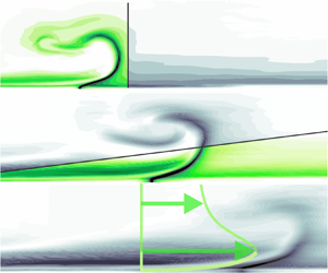
The mechanism of streamwise vorticity amplification through vortex-line bending is illustrated in figure 7 where spanwise velocity profiles measured at an outlet distance of  $x/b=600$ are shown for the cases with and without co-flow. Both profiles are extracted from the locations where
  $|w|$ reaches its maximum in the
  $z/b>0$ half-plane. Note that positive values indicate outward-directed flow.

Figure 7. Profiles of spanwise velocity component  $w$ at
  $x/b=600$ in
  $z/b>0$ half-plane at the location of maximum
  $w$: (a)
  $U_\infty = 20\,{\rm m}\,{\rm s}^{-1}$ and (b) zero co-flow (
 $U_\infty = 0\,{\rm m}\,{\rm s}^{-1}$). The sign of streamwise vorticity amplification through vortex-line bending is highlighted for inner and outer layers of wall jets.
Comparing the cases with and without co-flow (figure 7a,b), it is confirmed that the spanwise component is of opposite sign throughout the presented velocity profiles (and indeed throughout the entire half-plane, not shown here). The maximum magnitude is reached at approximately  $Y_m$ for both cases where
  $\partial u/\partial y$, and thus the vorticity amplification, changes its sign.
We conclude that the presence of a co-flowing external stream fundamentally changes the spreading characteristics of steady wall jets. Specifically, streamwise vorticity with an opposite sense of rotation is produced, leading to the amplification of inward-directed lateral flow. This mechanism opposes the jet expansion in the spanwise direction through turbulent diffusion, apparently cancelling one another as a negligible overall spreading rate is measured. These findings are consistent with the ‘directing influence’ of the external stream noted by Narasimha et al. (Reference Narasimha, Narayan and Parthasarathy1973) and explain the applicability of scaling laws determined for the two-dimensional flow to jet properties inside the symmetry plane of the finite-span jets addressed in the current study.
3.2. Starting finite-span wall jet
Next, we consider the case where the jet emission is started at a defined time instant, which was realised by opening the fast-switching valve at  $t = t_0$. The practical consideration that such a
  $t_0$ also exists for experiments of steady jets addressed above suggests that ‘approximate self-similarity’ may also be observed for starting wall jets provided the flow is assessed after a sufficiently long time duration. The main objective in this subsection is to determine this time delay or, from a different perspective, identify the region inside the leading part of starting wall jets where the scaling method introduced above is not applicable.
Figure 8 contains information on velocity fields during the starting process based on phase-locked PIV measurements. Contour plots of the steady wall jets are also shown in the bottom row for reference. The presented quantities are the same as in figure 3 but only the medium velocity ratio wall jet ( $R=0.67$) is shown.

Figure 8. Time series of gain in streamwise velocity due to  $R=0.67$ starting wall jets (a) and mean spanwise vorticity (b).
Following the fluid emission, a leading vortex develops. This flow structure is associated with an accumulation of spanwise vorticity, inducing a gain in near-wall velocity as well as a slight deficit in the outer layer. As shown by the authors through tomographic reconstructions of the three-dimensional flow field (Steinfurth & Weiss Reference Steinfurth and Weiss2021a,Reference Steinfurth and Weissc), the leading vortex has the shape of a half-ring in the case of finite-span outlet slots. As this vortex half-ring propagates downstream, it quickly diffuses due to viscous shearing. It is important to note that the spreading rate near the propagation front is larger than in the trailing wall-attached jet, i.e. peak jet velocities  $U_m$ are found in greater wall distance. Apart from the leading vortex, however, the wall jet appears to exhibit similar characteristics to the steady wall jet addressed above. It is therefore reasonable to assume that similarity behaviour, shown to be at hand for the steady configuration, also exists for certain regions of starting wall jets.
In order to quantitatively define flow regions where ‘approximate self-similarity’ may be applicable, more information regarding the convection of the propagation front is required. As a means to reveal the leading vortex ring, a series of finite-time Lyapunov exponent (FTLE) fields are shown in figure 9. Large values of this quantity indicate an attracting material line (A), governing the displacement of boundary-layer fluid along the propagation front. Figure 9 also contains diagrams of  $U_m$ and
  $Y_m$ extracted for the same time steps. Interestingly, jet parameters approach values associated with steady wall jets in the flow region between outlet and leading part of the jet. Across the leading vortex (with increasing
  $x$), however, a departure from the steady wall jet behaviour is noted as
  $Y_m$ points to locations outside the boundary layer downstream of the wall jet. The departure of
  $Y_m$ curves from the steady case is highlighted by dashed verticals, coinciding with the trailing ends of vortex structures revealed by FTLE fields. We therefore use the time-dependent locations where
  $Y_m$ starts to deviate from the steady jet curve as a measure for the convection of the leading vortex in the following. To this end, threshold values are applied to curves of starting wall jets for different time instants. Specifically, we define the location of the propagation front
  $x_p$ as the smallest
  $x$ where
  $Y_m$ deviates by more than 20 % from the value for the steady wall jet. Illustrating the identification of the propagation front, supplementary movie 1 available at https://doi.org/10.1017/jfm.2022.858 shows the time-dependent FTLE field (top) and the development of
  $Y_m(x/b,t)$ (bottom) for the
  $R=0.67$ starting jet. The location
  $x_p$ is highlighted by a red marker in the bottom and a dashed line in the top diagram. Note that the video contains more time steps than measurement phases since a temporal interpolation using the method proposed by Akima (Reference Akima1970) has been applied.

Figure 9. (a) Time series of FTLE fields for  $R=0.67$ starting wall jet. (b) Peak jet velocities with respective wall distance for the same time steps as in (a). The dashed verticals highlight the time-dependent boundary between wall jet and leading vortex indicated by the departure of
  $Y_m$ from the curve for the steady wall jet.
The time-dependent locations of the propagation front  $x_p$ are detected in an analogous fashion for the remaining velocity ratios. Along with linear fits that approximate the values with minimum mean squared deviation (dashed lines), they are shown in the space–time diagram in figure 10(a). The slopes stated in the figure may be viewed as measures of the convective velocities.

Figure 10. Time-dependent locations of boundary between leading vortex and starting wall jet for different velocity ratios. Linear fits are highlighted by dashed lines. (a) Locations as a function of time and (b) locations scaled with  $R$.
$R$.
It is immediately apparent that the convective velocity depends on the velocity ratio. This suggests the application of  $R$ as a scaling parameter, which was also proven to be a good choice to describe the evolution of main wall jet properties above. And indeed, the curves of time-dependent locations of the jet leading part collapse reasonably well onto a linear curve characterised by a normalised convective velocity of
  $U_p = 1.48RU_\infty$ (figure 10b).
We now use this approximation to identify the region spanned by the wall jet for various time steps during the starting process. For PIV data, yielding  $U_m$,
  $Y_m$ and
  $Y_{m/2}$, the convective velocity simply defines intervals of
  $x/b$. For wall shear stress measurements, where the number of temporal samples by far exceeds the number of sensors, we use
  $U_p$ to compute residence times of the wall jet regions at the respective sensor locations. The scaled jet properties, along with the power-law expressions determined for steady wall jets above (solid line), are presented in figure 11. Symbols coloured in grey indicate the region
  $x>x_{p}$ that lies downstream of the propagation front according to the threshold defined above.

Figure 11. Scaled starting wall jet properties for different time instants. Black symbols are used for the region upstream of leading vortex and grey symbols for the region further downstream.
As hypothesised above, there is indeed a wall jet region during the starting process with characteristics identical to those of steady wall jets. The scatter observed for black circles is not larger than that for the steady-blowing case. Deviations from the power-law fit are again due to an insufficient local momentum excess. Furthermore, we conclude that the approximate convective velocities are suited to determine the flow region where the scaling suggested by ZW93 can be applied. A distinct departure from the ‘approximately self-similar’ behaviour is only noted across the leading vortex region, i.e. when  $x>x_p$ (grey symbols).
3.3. Stopping finite-span wall jet
Attention is now turned to the case where the fluid emission is terminated at  $t = t_{p}$. Prior to that time instant, the flow field is identical to that of a steady wall jet addressed above.
A time series of the velocity fields directly subsequent to the end of the jet emission is presented in figure 12. Again, only the medium velocity ratio  $R=0.67$ is considered, for which the gain in streamwise velocity (figure 12a) and the spanwise vorticity (figure 12b) are shown.

Figure 12. Time series of gain in streamwise velocity due to  $R=0.67$ stopping wall jet (a) and mean spanwise vorticity (b).
Immediately following the jet emission phase, a stopping vortex is generated near the outlet. This flow structure has been observed previously by Steinfurth & Weiss (Reference Steinfurth and Weiss2021a) and was explained as a consequence of radial entrainment at the jet trailing part due to mass conservation. It is associated with a small-scale strand of positive spanwise vorticity, inducing a slight velocity deficit on its upper part before diffusing quickly. At larger  $x/b$, however, both the velocity and vorticity fields appear to be very similar to that of the steady jet.
This is confirmed by the diagrams presented in figure 13, showing peak jet velocities  $U_m$ and corresponding jet widths
  $Y_m$ during the stopping process. Both parameters again converge to the values measured for the steady wall jet for large
  $x/b$. The jet trailing part, however, represents a deceleration wave featuring smaller maximum velocities
  $U_m$.

Figure 13. (a) Peak jet velocities  $U_m$ and (b) respective wall distance
  $Y_m$ for
  $R=0.67$ stopping wall jet for different time steps subsequent to the termination of fluid emission at
  $t=t_p$.
Compared with  $Y_m$,
  $U_m$ appears to be the more sensitive indicator of the transitional region between deceleration wave and jet with steady characteristics. We therefore evaluate time-dependent
  $U_m$ distributions to detect the upstream boundary of the ‘approximately self-similar’ flow region coinciding with the global maximum in
  $U_m$ by definition. This choice is motivated by the monotonic decrease in streamwise direction for the steady wall jet and the empirical observation that both
  $U_m$ and
  $Y_m$ curves collapse downstream of the location associated with maximum velocity as shown in figure 13. Supplementary movie 2 illustrates the extraction of the deceleration wave location denoted
  $x_d$, highlighted by a red marker in the bottom and a dashed line in the top diagram of the movie. Again, the movie contains more time steps than measurement phases since a temporal interpolation has been applied.
The time-dependent locations  $x_d$ for the three velocity ratios are presented in figure 14. Note that the dashed lines again indicate linear fits for the measurement data, reflecting the advancing velocity of the deceleration wave.

Figure 14. Time-dependent locations of deceleration wave for stopping wall jets of different velocity ratios. Linear fits are highlighted by dashed lines. (a) Locations as a function of time and (b) locations scaled with  $R$.
$R$.
An almost linear dependence can be noted inside the evaluated range. However, the associated velocities are much larger than those for the convection of the leading vortex, separated by a factor of approximately two. Also exceeding local streamwise velocities, it is reasonable to assume that the slopes of these curves are linked to the diffusion of the jet trailing part rather than its convection. Again, the velocity ratio  $R$ is applied to collapse the data for different jet velocities, yielding an approximate
  $U_{d} = 2.78RU_\infty$ for the advancing speed of the deceleration wave.
Based on this velocity, we identify a region inside the measurement domain that may exhibit behaviour similar to that of the steady wall jets addressed above. Figure 15 contains diagrams of the scaled jet properties with black symbols used for the region downstream of the locations estimated by  $U_d$. Again, both the decay of
  $U_m$ and
  $\tau$ as well as the jet spreading rate for these regions are in good agreement with the power-law expressions established above. Upstream of the jets, the velocity and wall shear stress decrease as values associated with the free stream are approached across the deceleration wave. This deviation from the ‘approximate self-similarity’ is adequately captured by employing
  $U_d$.

Figure 15. Scaled stopping wall jet properties for different time instants. Black symbols are used for the region downstream of deceleration wave and grey for deceleration wave and unforced boundary layer upstream of the wall jet.
3.4. A model for starting/stopping wall jets
The results presented so far indicate that power-law expressions proposed by Narasimha et al. (Reference Narasimha, Narayan and Parthasarathy1973) and ZW93 are also applicable to steady wall jets ejected from a finite-span nozzle after minor adjustments (3.4a–d). Interestingly, a jet structure with such characteristics is also found for unsteady jet velocity programmes, upstream of the propagation front ( $x_p$) and downstream of the deceleration wave (
 $x_d$), with time-dependent locations given by
 \begin{equation} x_{p}(t) = U_pt \end{equation}
and
 \begin{equation} x_{d}(t) = U_d \tilde{t}, \end{equation}
where
 \begin{equation} \tilde{t} =\begin{cases} 0\,\mathrm{s}, & \mathrm{if}\ t\leq t_{p} \\ t-t_{p}, & \mathrm{if}\ t> t_{p}. \end{cases} \end{equation}
Note that the propagation front exists for  $t\geq 0\,\mathrm {s}$, and the deceleration wave only starts to develop when
  $t$ equals the pulse duration
  $t_{p}$, i.e. when the fluid emission is stopped.
Now, a simple model for starting/stopping, or pulsed, wall jets can be introduced, predicting  $U_m$,
  $\tau$,
  $Y_m$ and
  $Y_{m/2}$ for outlet distances in the range
  $x=x_d,\ldots,x_p$. We now demonstrate the capabilities of this model by comparing the estimated peak jet velocities
  $U_m$ and the corresponding wall distances
  $Y_m$ with the measurement data for a pulse duration of
  $t_p = 11\,\mathrm {ms}$ (figure 16). For reasons of clarity, only the medium velocity ratio
  $R=0.67$ is shown for
  $Y_m$ models (figure 16d–f).

Figure 16. Comparison between measurement data (black curves) and modelled jet properties (red curves) for pulsed wall jet with duration  $t_{p}=11\,\mathrm {ms}$. (a–c) Velocity distributions for
  $R=(0.5, 0.67, 0.75)$. (d–f) Locations of maximum velocity for
  $R=0.67$.
The starting process is ongoing for the first two time steps, i.e. the trailing part of the jet is located at  $x/b=0$. A reasonable agreement between modelled and measured velocities can be attested although some deviation is observed for the two smaller velocity ratios at large outlet distances. This is explained by an insufficient excess in kinematic momentum flux preventing the applicability of the concept of ‘approximate self-similarity’. In fact, unrealistic maximum velocities
  $U_m < U_\infty$ are predicted for
  $R=0.5$ at
  $x/b>300$. For
  $R=0.75$, on the other hand, only minor deviations are noted. Furthermore, a good prediction of the jet leading part can be attested as larger rates of velocity decay are found downstream of the predicted jet propagation front, i.e. right of the red curves. Similarly, a good prediction of the decay in
  $U_m$ is noted for the largest velocity ratio during the stopping process in the jet far field. Substantial deviations, however, are observed for the smaller velocity ratio as the excess in momentum flux is much smaller than
  $U_m/U_\infty = 2$, the threshold stated by ZW93.
A reasonable agreement between measurement data and modelled distributions is also at hand for  $Y_m$ where deviations merely occur in the sub-millimetre range. This is also the case for the two other velocity ratios that are not included in the figure.
Finally, we use the proposed model to estimate the wall shear stress signals at five locations downstream of the outlet, again considering pulsed jets with a valve opening time of  $t_p=11\,\mathrm {ms}$ (figure 17). Here,
  $U_p$ and
  $U_d$ are used to determine the time intervals during which the wall jets reside at the sensor locations. Note that the introduced model predicts constant jet properties at given outlet distances for each jet velocity. Therefore, the modelled signals equal horizontals with end points depending on
  $U_p$ and
  $U_d$.

Figure 17. Measured wall shear stress signals (black curves) and modelled wall shear stress (red curves) for pulsed wall jet with duration  $t_{p}=11\,\mathrm {ms}$ at five locations downstream of jet outlet.
Since  $U_d$ is almost twice as large as
  $U_p$, a decreasing length of the wall jet
  $x_p - x_d$ is predicted as it convects downstream. At
  $R=0.5$, this difference is only positive for the first three sensor locations. In other words, complete diffusion of the wall jet is predicted before reaching larger outlet distances. Indeed, no clear plateaus are seen in the signals measured at these locations. For the two larger velocity ratios, small jet lengths are estimated in the jet far field which is again confirmed by the phase-averaged signals. The actual passage of wall jets inducing quasi-constant wall shear stress appears to slightly forego the prediction by the model which is due to the conservative definition of the ‘approximately self-similar’ jet region based on the threshold values stated above. Nonetheless, a reasonable overall agreement between the modelled and measured wall shear stress can be attested during the jet passage with mean deviations per velocity ratio not exceeding 10 %.
4. Conclusions
The main objective of this study was to assess the applicability of scaling laws established by Narasimha et al. (Reference Narasimha, Narayan and Parthasarathy1973) to pulsed finite-span wall jets in a co-flowing external stream. A pulsed-jet actuator was used to generate jets with a constant velocity as well as unsteady velocity programmes.
Despite the limited spanwise outlet dimension,  $L=20\,\mathrm {mm}$, non-dimensional velocity profiles identical to those of two-dimensional wall jets studied by ZW93 are determined in the centre plane. There is a small discrepancy for the smallest investigated velocity ratio
  $R=0.5$, which is in line with empirical observations made by ZW93 suggesting that a certain excess in momentum flux is required for wall jets to exhibit ‘approximate self-similarity’. This was confirmed in the current study where power-law expressions similar to those obtained by ZW93 were shown to map the development of the decay in maximum velocity and wall shear stress as well as the jet spreading rate for larger velocity ratios
  $R=(0.67, 0.75)$. These scaling laws only require knowledge of the gross momentum flux in the outlet plane, the jet velocity ratio and the kinematic viscosity. Previous investigations of finite-span wall jets indicate what Narasimha et al. (Reference Narasimha, Narayan and Parthasarathy1973) dubbed ‘anomalous behaviour’ due to three-dimensional effects (Sforza & Herbst Reference Sforza and Herbst1970; Newman et al. Reference Newman, Patel, Savage and Tjio1972), mainly reflected in enhanced lateral spreading and thus a more rapid velocity decay. However, such characteristics have only been observed in the absence of a co-flow (Davis & Winarto Reference Davis and Winarto1980; Abrahamsson et al. Reference Abrahamsson, Johansson and Löfdahl1996). Indeed, the strong lateral spreading for this case was confirmed through PIV measurements up to
  $x/b=600$ in the current study but a different picture was revealed when an external stream was applied. Here, the spanwise velocity component is directed towards the jet symmetry plane while the wall-normal component is associated with an outward-directed fluid motion. In consequence, a self-amplifying process of streamwise vorticity production that is argued to be responsible for the large lateral spreading rates without an external stream by Launder & Rodi (Reference Launder and Rodi1983) and George et al. (Reference George, Abrahamsson, Eriksson, Karlsson, Löfdahl and Wosnik2000) is at hand. However, it is associated with an opposite sense of rotation, essentially countering the lateral spreading of the three-dimensional wall jet in the present set-up. This finding is consistent with what Narasimha et al. (Reference Narasimha, Narayan and Parthasarathy1973) referred to as the ‘directing influence’ of an external stream.
It was then shown that ‘approximately self-similar’ flow regions also exist in the case of starting and stopping wall jets where the momentum addition is initiated and stopped abruptly. These regions are enclosed by the leading vortex and the deceleration wave across which the flow properties transition to conditions found in the unforced boundary layer downstream and upstream of the wall jet, respectively. The velocities associated with these jet boundaries collapse when scaled with the velocity ratio parameter, which enables a prediction of the time-dependent wall jet region by means of empirical constants. It is worth mentioning that the advance of the deceleration wave is associated with a velocity approximately twice as large as the convective velocity of the jet leading part. Hence, the length of the region with steady jet characteristics decreases once the fluid emission is stopped, which is in agreement with less distinct footprints of wall jets for relatively short pulse durations noted by Steinfurth & Weiss (Reference Steinfurth and Weiss2021b). Based on the empirical constants, a model for wall jet properties is proposed, predicting the space–time interval where the wall jet resides. In this region, the maximum velocity, wall shear stress and spreading rate can be estimated using the scaling laws obtained for the steady configuration.
The model proposed in this article may prove useful in technical implementations of steady and unsteady finite-span wall jets. For instance, film cooling applications may benefit from estimations of the decay in wall shear stress that can be related to the local heat transfer. This may help in choosing an adequate supply mass flow and determine more appropriate locations of cooling holes. A further potential field of application lies in the active control of flow separation through pulsed blowing. Here, forcing parameters may be optimised to ensure a certain momentum addition throughout the control domain. However, it is reasonable to assume that wall jets exhibit different advancing velocities in such configurations compared with the zero-pressure-gradient flow addressed in this study. Future work therefore must be aimed at overcoming the empiricism related to the time-dependent wall jet boundaries. Furthermore, it remains unclear whether the quasi-two-dimensional flow can be maintained for even larger velocity ratios ( $U_j/U_\infty > 7$), i.e. when the flow approaches the case of relatively still surroundings. This issue should therefore be addressed in the future.
Supplementary movies
Supplementary movies are available at https://doi.org/10.1017/jfm.2022.858.
Funding
The authors gratefully acknowledge financial support from the Deutsche Forschungsgemeinschaft (DFG, German Research Foundation) under project number 426637148.
Declaration of interests
The authors report no conflict of interest.


