


1. Introduction
The lifetimes of foams and surface bubbles are primarily governed by the drainage and rupture processes of the thin liquid films surrounding bubbles. These processes are influenced by various intricate – and sometimes difficult to control – factors, including contamination Lhuissier & Villermaux (Reference Lhuissier and Villermaux2012), physicochemical properties of added surfactants (Petkova et al. Reference Petkova, Tcholakova, Chenkova, Golemanov, Denkov, Thorley and Stoyanov2020), evaporation Pasquet et al. (Reference Pasquet, Boulogne, Sant-Anna, Restagno and Rio2022), biomolecules (Choudhury et al. Reference Choudhury, Dey, Dixit and Feng2021) and history of thin film formation (Klaseboer et al. Reference Klaseboer, Chevaillier, Gourdon and Masbernat2000; Zawala et al. Reference Zawala, Miguet, Rastogi, Atasi, Borkowski, Scheid and Fuller2023), which may induce variations in lifetimes over several orders of magnitude. In the presence of surface-active species, a comprehensive description of the drainage of thin films is made difficult even in controlled conditions, particularly because of the coupling of flow with the concentration field of the species. Further complexity arises from the timescales of surface and bulk exchanges of surfactant, which can be comparable to the drainage time (Petkova et al. Reference Petkova, Tcholakova and Denkov2021). Generally, the surface rheology that results from those effects is accounted for by using a velocity boundary condition corresponding to an immobile interface with air (Aradian et al. Reference Aradian, Raphael and De Gennes2001), leading to a Poiseuille flow within the film. Although this is a fair assumption for an interface with concentrated surfactants, culminating in a simple lubrication equation for film thickness, it decouples the interfacial shear-stress from the bulk flow caused by drainage. Imposing mobile interfaces, and accounting for the continuity of tangential stress, one can obtain an integro-differential equation for filmheight (Yiantsios & Davis Reference Yiantsios and Davis1990). However, inclusion of additional Marangoni stress necessitates additional evolution equations for closure. This has been done in the past to some extent (Chan et al. Reference Chan, Klaseboer and Manica2011; Frostad et al. Reference Frostad, Walter and Leal2013) where the parabolic flow is coupled with empirical surface tension variations. Breward & Howell (Reference Breward and Howell2002) present a mathematically robust model for a linear variation of surface tension with surfactant concentration, an approximation that is valid only for dilute solutions. The complex surface rheology generally exhibited by surfactant solutions prevents the universality of models.
Recently, the foaming of oil mixtures has attracted renewed interest (Chandran Suja et al. Reference Chandran Suja, Kar, Cates, Remmert, Savage and Fuller2018; Lombardi et al. Reference Lombardi, Roig-Sanchez, Bapat and Frostad2023). The relatively stable foams that can form in these mixtures without any surfactant have been evidenced decades ago (Ross & Nishioka Reference Ross and Nishioka1975) and are currently observed in many processes of the oil industry, for example, car tank filling and crude oil extraction, or in the food industry, for instance, in frying oils. Anti-foaming molecules are then often required to increase efficiency (Pugh Reference Pugh1996). In the absence of evaporation, it has been shown that the enhanced lifetimes of thin films in mixtures stem from slight differences between the bulk and surface concentrations of different species, leading to thickness-dependent surface tensions of thin films (Tran et al. Reference Tran, Arangalage, Jørgensen, Passade-Boupat, Lequeux and Talini2020, Reference Tran, Passade-Boupat, Lequeux and Talini2022). Since the diffusion times of small molecules are very short, bulk and interfaces can be considered to be in thermodynamical equilibrium (the time for a molecule to travel across the thickness of a film is
 $h^2/D\sim 1\,\rm ms$
for a
$h^2/D\sim 1\,\rm ms$
for a
 $1\mathrm{-}\unicode{x03BC}\rm m$
-thick film and taking a typical diffusion coefficient,
$1\mathrm{-}\unicode{x03BC}\rm m$
-thick film and taking a typical diffusion coefficient,
 $D\sim 10^{-9}\rm m^2\,s^-{^1}$
). Thus, the surface rheology of mixtures reduces to Gibb’s elasticity (Tempel et al. Reference Tempel, Lucassen and Lucassen-Reynders1965). It leads to an increasing surface tension of a film with decreasing thickness. Since the concentration differences at stake remain very small, the variation of surface tension with concentration is linear. In addition, the disjoining pressure in a film is purely attractive, therefore binary oil mixtures constitute much simpler systems than surfactant solutions to study the drainage mechanisms of liquid films. Existing models developed for the pinching of films of surfactant solutions cannot predict quantitative lifetimes observed in thin films of binary mixtures (Tran et al. Reference Tran, Passade-Boupat, Lequeux and Talini2022).
$D\sim 10^{-9}\rm m^2\,s^-{^1}$
). Thus, the surface rheology of mixtures reduces to Gibb’s elasticity (Tempel et al. Reference Tempel, Lucassen and Lucassen-Reynders1965). It leads to an increasing surface tension of a film with decreasing thickness. Since the concentration differences at stake remain very small, the variation of surface tension with concentration is linear. In addition, the disjoining pressure in a film is purely attractive, therefore binary oil mixtures constitute much simpler systems than surfactant solutions to study the drainage mechanisms of liquid films. Existing models developed for the pinching of films of surfactant solutions cannot predict quantitative lifetimes observed in thin films of binary mixtures (Tran et al. Reference Tran, Passade-Boupat, Lequeux and Talini2022).
In the presence of Marangoni effects, the process of film drainage and rupture may be divided into three stages (Lhuissier & Villermaux Reference Lhuissier and Villermaux2012). The first stage comprises the thin film formation; from spherical surfaces to locally flat surfaces. In the case of binary mixtures, this shape is described using a mechanism of equilibration of film tension by a balance between surface tension gradient and the pressure gradient due to Laplace pressure difference. This is reached in a few milliseconds. Naturally, a second stage dynamics ensues, relaxing the pressure gradient and resulting in a more complicated film drainage scenario. The relaxation causes the film to drain via dimpled (marginal) pinching, as also described in soap films (Aradian et al. Reference Aradian, Raphael and De Gennes2001; Trégouët & Cantat Reference Trégouët and Cantat2021). At one point, the film becomes so thin that a third stage of van der Waals attraction becomes effective and causes spontaneous rupture (Shah et al. Reference Shah, Kleijn, Kreutzer and Van Steijn2021). The film lifetime is mostly determined by the second stage of film drainage when a pinched part reaches a critical thickness, which is much longer than the initial viscous stretching phase and the final spontaneous rupture due to van der Waals interactions.
In this article, we model the first two stages of marginal pinching of films of binary mixtures. We follow a similar approach as Breward & Howell (Reference Breward and Howell2002) and we do not impose immobile interfaces a priori, but instead we consider the coupling of the flow and concentration fields of species. Taking profit of the well-controlled physico-chemistry of mixtures, we obtain an evolution equation for surface tension, here in the context of binary mixtures, using thermodynamic principles of ideal solution theory. As a result, the parameters defining the surface tension gradient are fully determined by the chosen bulk concentration of the mixture species. The pinching dynamics is thus described by three one-dimensional (1-D) coupled evolution equations for film thickness
 $h$
, mean flow velocity
$h$
, mean flow velocity
 $\overline {u}$
and surface tension
$\overline {u}$
and surface tension
 $\gamma$
, which allows a quantitative description of the drainage of thin films and the prediction of their lifetimes.
$\gamma$
, which allows a quantitative description of the drainage of thin films and the prediction of their lifetimes.
The article is structured as follows. Section 2 introduces the conservation laws used to model the Marangoni-stress driven system. Section 3 showcases the detailed derivation of the closed-form model using three small parameters in the problem. Further, details of the numerical simulations are described and validated. In § 4, we discuss the main findings of the simulations, specifically focusing on: (i) film tension equilibration and (ii) drainage driven by Marangonistresses generated due to binary mixtures concentration differences. We elucidate our model predictions in comparison with film-thinning laws reported in past experiments/scaling theories, and also contrast with other models in the limiting cases. Finally, we put things into perspective and conclude in § 5.

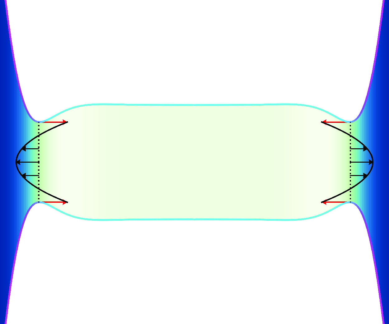
Figure 1. For the scope of this study, we consider a ligament of fluid pinned between two walls at a distance
 $\mathcal {L}$
. Initially, a flat-film profile of thickness,
$\mathcal {L}$
. Initially, a flat-film profile of thickness,
 $h_i=500\,\rm nm$
, is prescribed in the middle (spanning over
$h_i=500\,\rm nm$
, is prescribed in the middle (spanning over
 $\mathcal {L}/2=0.2\,\rm mm$
) conjoined to a Plateau border of radius,
$\mathcal {L}/2=0.2\,\rm mm$
) conjoined to a Plateau border of radius,
 $R_b=1\,\rm mm$
, using experimental estimations taken from Tran et al. (Reference Tran, Passade-Boupat, Lequeux and Talini2022). Using these constraints, we obtain
$R_b=1\,\rm mm$
, using experimental estimations taken from Tran et al. (Reference Tran, Passade-Boupat, Lequeux and Talini2022). Using these constraints, we obtain
 $\mathcal {H}\simeq 16\,\unicode{x03BC}\rm m$
.
$\mathcal {H}\simeq 16\,\unicode{x03BC}\rm m$
.
2. Governing equations
We consider a thin two-dimensional (2-D) liquid film of two miscible liquids, denoted as 1 and 2; the film is bounded by impenetrable walls at
 $x=\pm \mathcal {L}/2$
and free surfaces at
$x=\pm \mathcal {L}/2$
and free surfaces at
 $z=\pm h/2$
. Here,
$z=\pm h/2$
. Here,
 $\mathcal {L}$
is the prescribed length of the film and the interfaces are pinned at the walls with a height
$\mathcal {L}$
is the prescribed length of the film and the interfaces are pinned at the walls with a height
 $2\mathcal {H}$
as shown in figure 1. Since the volume of the film is too small for an equilibrium (parabolic) shape to be reached, the film has to drain and further rupture in the absence of any disjoining pressure. We model the drainage dynamics using conservative laws for mass, momentum and mixture species. In the following, we use subscripts
$2\mathcal {H}$
as shown in figure 1. Since the volume of the film is too small for an equilibrium (parabolic) shape to be reached, the film has to drain and further rupture in the absence of any disjoining pressure. We model the drainage dynamics using conservative laws for mass, momentum and mixture species. In the following, we use subscripts
 $(x,z,t)$
to denote derivatives
$(x,z,t)$
to denote derivatives
 $(\partial _x, \partial _z,\partial _t)$
in the equations.
$(\partial _x, \partial _z,\partial _t)$
in the equations.
2.1. Conservation of mass and momentum
For mass and momentum balance, we have the Navier–Stokes equations:
 \begin{align} u_x + v_z &= 0, \end{align}
 \begin{align} u_t + u u_x + v u_z &= - \frac {P_x}{\rho } + \frac {\mu }{\rho } [u_{x x} + u_{z z}], \end{align}
 \begin{align} v_t + u v_x + v v_z &= - \frac {P_z}{\rho } + \frac {\mu }{\rho } [v_{x x} + v_{z z}]. \end{align}
Here,
 $\rho$
and
$\rho$
and
 $\mu$
are the density and viscosity of the binary mixture which are kept constant;
$\mu$
are the density and viscosity of the binary mixture which are kept constant;
 $u$
and
$u$
and
 $v$
are the velocity components in the
$v$
are the velocity components in the
 $x$
- and
$x$
- and
 $z$
-directions, respectively. Considering the upper interface (
$z$
-directions, respectively. Considering the upper interface (
 $z=h/2$
), we have the jump conditions for a free interface. The normal stress balance reads as
$z=h/2$
), we have the jump conditions for a free interface. The normal stress balance reads as
 \begin{align} \boldsymbol {n\cdot \unicode{x1D64F}\cdot n} & = -\gamma \kappa , \end{align}
where
 $\unicode{x1D64F}=-P\boldsymbol{I}+\mu [\boldsymbol {(\nabla u) + (\nabla u)^T} ]$
is the stress tensor, the curvature of the free surface is given by
$\unicode{x1D64F}=-P\boldsymbol{I}+\mu [\boldsymbol {(\nabla u) + (\nabla u)^T} ]$
is the stress tensor, the curvature of the free surface is given by
 $\kappa =-({(h_{x x} / 2)}/{(1 + h_x^2 / 4)^{3 / 2}})$
and
$\kappa =-({(h_{x x} / 2)}/{(1 + h_x^2 / 4)^{3 / 2}})$
and
 $\boldsymbol{n}= ({1}/{[(1+h_x^2/4)^{1/2}])}([(- {h_x}/{2}),1])$
is the unit normal vector. It is written explicitly as
$\boldsymbol{n}= ({1}/{[(1+h_x^2/4)^{1/2}])}([(- {h_x}/{2}),1])$
is the unit normal vector. It is written explicitly as
 \begin{align} P - \mu \left [ \frac {[2 v_z (1 - h_x^2 / 4) - h_x (u_z + v_x) / 2]}{1 + h_x^2 / 4} \right ] & = \gamma \kappa . \end{align}
We also have the tangential stress balance:
 \begin{align} \boldsymbol {t\cdot \unicode{x1D64F}\cdot n} &= \nabla _s\gamma , \end{align}
where
 $\textbf {t}= ({1}/{[(1+h_x^2/4)^{1/2}]})([1, ({h_x}/{2})])$
is the unit tangential vector and
$\textbf {t}= ({1}/{[(1+h_x^2/4)^{1/2}]})([1, ({h_x}/{2})])$
is the unit tangential vector and
 $\nabla _s=[\textit{\textbf{I-nn}}]\boldsymbol {\cdot \nabla }$
is the curvilinear gradient operator along the interface. It is written explicitly as
$\nabla _s=[\textit{\textbf{I-nn}}]\boldsymbol {\cdot \nabla }$
is the curvilinear gradient operator along the interface. It is written explicitly as
 \begin{align} \mu (u_z + v_x) (1 - h_x^2 / 4)^{1 / 2} + \mu h_x (v_z - u_x) & = \gamma _x (1 + h_x^2 / 4)^{1 / 2}. \end{align}
Additionally, we have the kinematic equation for the free surface:
 \begin{equation} h_t + u h_x = 2 v. \end{equation}
Lastly, we take symmetry conditions at
 $z=0$
:
$z=0$
:
 \begin{equation} u_z = 0 ; \quad v = 0. \end{equation}
2.2. Conservation of species
For liquids with typical diffusion coefficient,
 $D\sim 10^{-9}\,\rm m^2s^-{^1}$
, the equilibrium between the interfaces and the bulk is attained very quickly (
$D\sim 10^{-9}\,\rm m^2s^-{^1}$
, the equilibrium between the interfaces and the bulk is attained very quickly (
 $h^2/D \simeq 10^{-5}\rm s$
for
$h^2/D \simeq 10^{-5}\rm s$
for
 $h=100\,\rm nm$
) as compared with the characteristic time scales of the problem – which range from
$h=100\,\rm nm$
) as compared with the characteristic time scales of the problem – which range from
 $10\,\rm ms$
to
$10\,\rm ms$
to
 $10\,\rm s$
. However, the lateral diffusion of species is slow (
$10\,\rm s$
. However, the lateral diffusion of species is slow (
 $L^2/D \simeq 10^3\,\rm s$
for
$L^2/D \simeq 10^3\,\rm s$
for
 $L=1\,\rm mm$
), so we can fairly neglect it. Consequently, we only take into account lateral advection of species and assume that the system is in thermal equilibrium at a given
$L=1\,\rm mm$
), so we can fairly neglect it. Consequently, we only take into account lateral advection of species and assume that the system is in thermal equilibrium at a given
 $x$
-location.
$x$
-location.
We also introduce the relation between species concentrations of the binary mixture film and its surface tension to couple the flow with the surface tension gradient. Subsequently, we derive an evolution equation for the surface tension based on a volume conservation law for the binary mixture.
Let
 $c_A$
be the molar fraction of species A (with the lower surface tension) in the bulk and
$c_A$
be the molar fraction of species A (with the lower surface tension) in the bulk and
 $\unicode{x1D6E4} _A$
be the corresponding molar fraction in the surface layer. Considering a finite thickness of the interface,
$\unicode{x1D6E4} _A$
be the corresponding molar fraction in the surface layer. Considering a finite thickness of the interface,
 $\delta \ll h$
, the particle numbers per area for species A in a thin differential element in
$\delta \ll h$
, the particle numbers per area for species A in a thin differential element in
 $x$
can be written as
$x$
can be written as
 $w_A=hc_A+2\delta \unicode{x1D6E4} _A$
. The flux can be expressed as
$w_A=hc_A+2\delta \unicode{x1D6E4} _A$
. The flux can be expressed as
 $j_A = c_A h \overline {u} + \unicode{x1D6E4} _A (2\delta )u_s$
, where
$j_A = c_A h \overline {u} + \unicode{x1D6E4} _A (2\delta )u_s$
, where
 $\overline {u}$
and
$\overline {u}$
and
 $u_s$
are mean bulk and interfacial velocities, respectively. Omitting the index A, and using subscripts to denote derivatives, the conservation law for particle numbers per area for species A is written as
$u_s$
are mean bulk and interfacial velocities, respectively. Omitting the index A, and using subscripts to denote derivatives, the conservation law for particle numbers per area for species A is written as
 \begin{equation} w_t = -j_x = -(c h \overline {u} + \unicode{x1D6E4} (2\delta )u_s)_x. \end{equation}
We use thermodynamics of ideal mixtures, using a relation known as Butler’s equation (Butler Reference Butler1932; Santos & Reis Reference Santos and Reis2021) to relate the surface molar fraction,
 $\unicode{x1D6E4} _i$
, to the bulk molar fraction
$\unicode{x1D6E4} _i$
, to the bulk molar fraction
 $c_i$
for the species
$c_i$
for the species
 $i$
in an infinite reservoir. Considering the same molar surface
$i$
in an infinite reservoir. Considering the same molar surface
 $\sigma _i$
for the two species for simplicity, we have
$\sigma _i$
for the two species for simplicity, we have
 \begin{equation} \unicode{x1D6E4} _i=c_i e^{(S (\gamma (c_i) -\gamma _i))}, \end{equation}
where
 $\gamma _i$
is the surface tension of pure liquid species
$\gamma _i$
is the surface tension of pure liquid species
 $i$
and
$i$
and
 $S={\sigma _i}/{RT}$
with
$S={\sigma _i}/{RT}$
with
 $RT$
being the molar thermal energy. Therefore,
$RT$
being the molar thermal energy. Therefore,
 $S (\gamma -\gamma _i)$
is the ratio of the energy cost to replace species
$S (\gamma -\gamma _i)$
is the ratio of the energy cost to replace species
 $i$
by the mixture at the interface to the thermal energy. For a two species mixture, we have
$i$
by the mixture at the interface to the thermal energy. For a two species mixture, we have
 $\unicode{x1D6E4} _A+\unicode{x1D6E4} _B=1$
and
$\unicode{x1D6E4} _A+\unicode{x1D6E4} _B=1$
and
 $c_A+c_B=1$
. This gives the interfacial tension for an infinite reservoir,
$c_A+c_B=1$
. This gives the interfacial tension for an infinite reservoir,
 \begin{equation} \gamma (c)= \gamma _B- \frac {\log \left [ 1+c(e^{S(\gamma _B-\gamma _A)}-1)\right ]}{S}, \end{equation}
where
 $c$
is the free variable for concentration such that
$c$
is the free variable for concentration such that
 $\gamma =\gamma _B$
for
$\gamma =\gamma _B$
for
 $c=0$
(pure species B) and
$c=0$
(pure species B) and
 $\gamma =\gamma _A$
for
$\gamma =\gamma _A$
for
 $c=1$
(pure species A). Hereafter, we use the index
$c=1$
(pure species A). Hereafter, we use the index
 $0$
for reference values at infinite film thickness. Equation (2.12) results in a sub-linear variation of surface tension with concentration, as observed in a wide range of binary mixtures. These variations will be later commented on, and shown in figure 2.
$0$
for reference values at infinite film thickness. Equation (2.12) results in a sub-linear variation of surface tension with concentration, as observed in a wide range of binary mixtures. These variations will be later commented on, and shown in figure 2.
3. Reduced order model
In the lubrication limit (
 $h_x\ll 1$
), we expand the flow variables
$h_x\ll 1$
), we expand the flow variables
 $(u,v,P)$
in a Taylor series with respect to
$(u,v,P)$
in a Taylor series with respect to
 $z$
. The horizontal velocity in the bulk is written as
$z$
. The horizontal velocity in the bulk is written as
 \begin{equation} u(x,z)=\overline {u}(x)+u_{Po}(z^2/h^2-1/12)+ O(z^4), \end{equation}
where we have intentionally assigned the leading and first-order velocities as
 $u^{(0)}=\overline {u}$
and
$u^{(0)}=\overline {u}$
and
 $u^{(2)}h^2=u_{Po}$
. This helps us to intuitively realise some quantities described by the species conservation law (2.10). The average velocity
$u^{(2)}h^2=u_{Po}$
. This helps us to intuitively realise some quantities described by the species conservation law (2.10). The average velocity
 $\overline {u}$
is responsible for the shape evolution of the film and the Poiseuille component of the velocity
$\overline {u}$
is responsible for the shape evolution of the film and the Poiseuille component of the velocity
 $u_{Po}$
(having by construction a zero mean value) is responsible only for the relative motion of the surface and the bulk, and thus for the non-uniform advection of species. The vertical velocity component
$u_{Po}$
(having by construction a zero mean value) is responsible only for the relative motion of the surface and the bulk, and thus for the non-uniform advection of species. The vertical velocity component
 $v$
is expanded using continuity (2.1) as
$v$
is expanded using continuity (2.1) as
 \begin{equation} v(x,z) = - \overline {u}_x z - (u_{Po})_x \left ( {z^3} / 3 h^2 - z / 12 \right ) + u_{Po} (2 h_x z^3 / 3h^3) +\mathcal {O} (z^5), \end{equation}
and the pressure as
 \begin{equation} P(x,z) = P^{(0)} + P^{(2)} \left ( {z^2} - h^2 / 12 \right ) +\mathcal {O} (z^4). \end{equation}
We put (3.1)–(3.3) into the governing equations for momentum and mass balance (2.1)–(2.9), and find a leading order problem with an unknown surface-tension field
 $\gamma (x,t)$
. Next, using a double expansion Taylor series for the surface tension (for small interfacial thickness and small variation in species concentration), we obtain an evolution equation for
$\gamma (x,t)$
. Next, using a double expansion Taylor series for the surface tension (for small interfacial thickness and small variation in species concentration), we obtain an evolution equation for
 $\gamma (x,t)$
using conservation of species (2.10). This provides closure to the leading order problem and consequently gives us a set of well-posed evolution equations for
$\gamma (x,t)$
using conservation of species (2.10). This provides closure to the leading order problem and consequently gives us a set of well-posed evolution equations for
 $h(x,t),\overline {u}(x,t)$
and
$h(x,t),\overline {u}(x,t)$
and
 $\gamma (x,t)$
.
$\gamma (x,t)$
.
3.1. Evolution equations for film thickness and averaged velocity
The following procedure for deriving the thin film hydrodynamics equations is in the spirit of the derivation first done in the seminal work of Eggers & Dupont (Reference Eggers and Dupont1994). Enforcing mass conservation of the film (2.1) into the kinematic equation (2.8) gives us the evolution equation for the film height (Leal Reference Leal2007), valid at all orders. We thus write the leading order kinematic equation as
 \begin{equation} h_t = -(h\overline {u}+2\delta u_s)_x \simeq -(h\overline {u})_x, \end{equation}
Using (3.1)–(3.3) in the x-momentum (2.2), we obtain at leading order,
 \begin{equation} \overline {u}_t + \overline {u} \overline {u}_x = - \frac {P_x^{(0)}}{\rho } + \frac {\mu }{\rho } \left (\overline {u}_{x x} + 2 \frac {u_{Po}}{h^2}\right ), \end{equation}
while the z-momentum (2.3) is identically satisfied. Similarly, the interfacial stress conditions given by (2.5) and (2.7) is written at the leading order as
 \begin{align} P ^{(0)} = & - \frac {\gamma h_{xx}}{2} - 2 \mu \overline {u}_x, \end{align}
 \begin{align} u _{Po} = &\frac {\gamma _xh}{\mu } + \frac {\overline {u}_{x x} h^2}{2} + 2 h h_x \overline {u}_x. \end{align}
Note here that the leading order tangential stress condition (3.6b
) is at
 $O(z)$
. Next, we eliminate
$O(z)$
. Next, we eliminate
 $P^{(0)}$
and
$P^{(0)}$
and
 $u_{Po}$
in (3.5) using (3.6a
) and (3.6b
), respectively, and neglect
$u_{Po}$
in (3.5) using (3.6a
) and (3.6b
), respectively, and neglect
 $\gamma _x h_{xx}$
with respect to
$\gamma _x h_{xx}$
with respect to
 $\gamma _0 h_{xxx}$
(small surface tension variation) and
$\gamma _0 h_{xxx}$
(small surface tension variation) and
 $2\gamma _x/h$
(
$2\gamma _x/h$
(
 $h_x \ll 1$
), finally obtaining
$h_x \ll 1$
), finally obtaining
 \begin{equation} \overline {u}_t + \overline {u}\overline {u}_x = \frac {1}{\rho h}\left (2\gamma _x+\frac {\gamma _0hh_{xxx}}{2}\right ) + \frac {\mu }{\rho }\frac {(4h \overline {u}_x)_x}{h}. \end{equation}
Here,
 $\gamma _0$
is the reference surface tension of the liquid mixture at infinite film thickness. We emphasise the subtle point that the 1-D equations (3.4) and (3.7) describes the 2-D velocity field
$\gamma _0$
is the reference surface tension of the liquid mixture at infinite film thickness. We emphasise the subtle point that the 1-D equations (3.4) and (3.7) describes the 2-D velocity field
 $u(x,z)$
. The second-order velocity term
$u(x,z)$
. The second-order velocity term
 $u_{Po}$
enters the leading order problem through (3.6b
) ensuring tangential stress balance at the interface. As discussed by Tran et al. (Reference Tran, Passade-Boupat, Lequeux and Talini2022), we have a constant film tension at mechanical equilibrium which differs from the interfacial tension. More precisely, in the limit of small curvatures and slopes, the film tension reads
$u_{Po}$
enters the leading order problem through (3.6b
) ensuring tangential stress balance at the interface. As discussed by Tran et al. (Reference Tran, Passade-Boupat, Lequeux and Talini2022), we have a constant film tension at mechanical equilibrium which differs from the interfacial tension. More precisely, in the limit of small curvatures and slopes, the film tension reads
 $C\,=\,\gamma (2- h_x^2/4 + h h_{xx}/2 )$
, which is the sum of the interfacial tension at small slopes (
$C\,=\,\gamma (2- h_x^2/4 + h h_{xx}/2 )$
, which is the sum of the interfacial tension at small slopes (
 $\cos \theta \simeq 1-h_x^2/8$
) and the force due to the Laplace pressure (
$\cos \theta \simeq 1-h_x^2/8$
) and the force due to the Laplace pressure (
 $\Delta P\simeq \gamma h_{xx}/2$
). The first term of the right-hand side of (3.7) can thus be identified as the gradient of film tension
$\Delta P\simeq \gamma h_{xx}/2$
). The first term of the right-hand side of (3.7) can thus be identified as the gradient of film tension
 $C$
at leading order in
$C$
at leading order in
 $h_x$
. The last term originates from the classical Trouton viscosity which is the ratio of elongational to shear viscosity for planar Newtonian viscous flows appropriate for thin films (Choudhury et al. Reference Choudhury, Paidi, Kalpathy and Dixit2020).
$h_x$
. The last term originates from the classical Trouton viscosity which is the ratio of elongational to shear viscosity for planar Newtonian viscous flows appropriate for thin films (Choudhury et al. Reference Choudhury, Paidi, Kalpathy and Dixit2020).
We now have the evolution equations for the film thickness
 $h(x,t)$
(3.4) and the average velocity
$h(x,t)$
(3.4) and the average velocity
 $\overline {u}(x,t)$
(3.7). To close the system, we need an equation for the unknown surface tension field
$\overline {u}(x,t)$
(3.7). To close the system, we need an equation for the unknown surface tension field
 $\gamma (x,t)$
. This is derived in the following subsection.
$\gamma (x,t)$
. This is derived in the following subsection.
3.2. Evolution equation for surface tension of binary mixtures
To obtain a consistent relation for the surface tension field
 $\gamma$
in terms of the species concentration
$\gamma$
in terms of the species concentration
 $c$
and film thickness
$c$
and film thickness
 $h$
, we need to define a new variable, the global molar fraction (averaged across
$h$
, we need to define a new variable, the global molar fraction (averaged across
 $z$
),
$z$
),
 \begin{equation} X(x,t) = \frac {w}{h+2\delta } = \frac {c h + 2 \unicode{x1D6E4} \delta }{h+2\delta }. \end{equation}
In the following, we will use the global molar fraction
 $X$
as the free variable for species concentration. In fact, if a homogeneous piece of film is stretched at a constant volume,
$X$
as the free variable for species concentration. In fact, if a homogeneous piece of film is stretched at a constant volume,
 $c$
and
$c$
and
 $\Gamma$
both vary because the surface to volume ratio of the film varies, while
$\Gamma$
both vary because the surface to volume ratio of the film varies, while
 $X$
remains constant. Thus, the variable
$X$
remains constant. Thus, the variable
 $X$
allows us to perform a more comprehensive derivation of the surface tension dependence on species concentration. Subsequently, an explicit relation between
$X$
allows us to perform a more comprehensive derivation of the surface tension dependence on species concentration. Subsequently, an explicit relation between
 $X$
and
$X$
and
 $\gamma$
can be deduced using (3.8) and (2.11) in (2.12), giving us the following expression:
$\gamma$
can be deduced using (3.8) and (2.11) in (2.12), giving us the following expression:
 \begin{equation} \gamma {(X,h)}= \gamma _B -\frac {1}{S} \log \left (\frac {X (2 \delta +h) e^{S(\gamma _B -\gamma _A)}}{h+2 \delta e^{S (\gamma -\gamma _A)}}-\frac {X (2 \delta +h)}{h+2 \delta e^{S (\gamma -\gamma _A)}}+1\right ). \end{equation}
Since the surface tension varies weakly during the whole pinching process (typically differences of
 $10^{-3}\gamma _0$
are involved in these phenomena Tran et al. Reference Tran, Arangalage, Jørgensen, Passade-Boupat, Lequeux and Talini2020), we can linearly expand the surface tension of the film. Considering the reference surface tension
$10^{-3}\gamma _0$
are involved in these phenomena Tran et al. Reference Tran, Arangalage, Jørgensen, Passade-Boupat, Lequeux and Talini2020), we can linearly expand the surface tension of the film. Considering the reference surface tension
 $\gamma (X_0,\infty )=\gamma _0=\gamma (c_0)$
, with
$\gamma (X_0,\infty )=\gamma _0=\gamma (c_0)$
, with
 $c_0=X_0$
, we substitute
$c_0=X_0$
, we substitute
 $\gamma _0=\gamma (c_0)$
for
$\gamma _0=\gamma (c_0)$
for
 $\gamma$
on the right-hand side of (3.9) using (2.12). Next, we expand it using Taylor series both in
$\gamma$
on the right-hand side of (3.9) using (2.12). Next, we expand it using Taylor series both in
 $\delta$
and (
$\delta$
and (
 $X - X_0$
),
$X - X_0$
),
 $X_0$
being the initial uniform (global) molar fraction. This gives the following exact result at first order in
$X_0$
being the initial uniform (global) molar fraction. This gives the following exact result at first order in
 $\delta$
and (
$\delta$
and (
 $X-X_0$
):
$X-X_0$
):
 \begin{equation} \gamma {(X,h)} = \gamma _0+\frac {\delta }{h}\frac {2 (1-X_0) X_0 \left (e^{S\Delta \gamma }-1\right )^2}{ S \left (1+X_0(e^{S\Delta \gamma }-1)\right )^2} -(X-X_0)\frac {e^{S\Delta \gamma }-1}{S(1+ X_0 \left (e^{S\Delta \gamma }-1\right ))}, \end{equation}
where
 $\Delta \gamma =\gamma _B-\gamma _A$
. We thus have the linearised version of
$\Delta \gamma =\gamma _B-\gamma _A$
. We thus have the linearised version of
 $\gamma$
:
$\gamma$
:
 \begin{equation} \gamma {(X,h)} = \gamma _0\left (1 + \frac {\alpha }{h} - \beta \left (X-X_0 \right )\right ). \end{equation}
The term
 $\alpha \gamma _0 /h$
is the Gibbs elastic modulus of the film, or the variation of the interfacial tension under stretching at constant global molar fraction
$\alpha \gamma _0 /h$
is the Gibbs elastic modulus of the film, or the variation of the interfacial tension under stretching at constant global molar fraction
 $X$
(see discussions of Tran et al. Reference Tran, Arangalage, Jørgensen, Passade-Boupat, Lequeux and Talini2020,Reference Tran, Passade-Boupat, Lequeux and Talini2022) whereas
$X$
(see discussions of Tran et al. Reference Tran, Arangalage, Jørgensen, Passade-Boupat, Lequeux and Talini2020,Reference Tran, Passade-Boupat, Lequeux and Talini2022) whereas
 $\beta$
is a positive dimensionless solutal Marangoni coefficient. Both
$\beta$
is a positive dimensionless solutal Marangoni coefficient. Both
 $\alpha$
and
$\alpha$
and
 $\beta$
depend on the initial composition of the mixture. Combining (2.11) and (2.12), and using (3.8), we also have
$\beta$
depend on the initial composition of the mixture. Combining (2.11) and (2.12), and using (3.8), we also have
 \begin{equation} \unicode{x1D6E4} _0-c_0=\frac {(1-X_0) X_0 \left (e^{S\Delta \gamma }-1\right )}{1 + X_0 \left (e^{S\Delta \gamma }-1\right )}, \end{equation}
which leads to
 \begin{equation} \beta =\frac {1}{\gamma _0 S} \frac {\unicode{x1D6E4} _0-c_0}{X_0(1-X_0)}=\frac {1}{\gamma _0}\frac {\partial \gamma }{\partial c_0} \end{equation}
and to
 \begin{equation} \alpha =2\delta (\unicode{x1D6E4} _0-c_0)\beta . \end{equation}

Figure 2. Variation of
 $\gamma (c_A)$
,
$\gamma (c_A)$
,
 $(\unicode{x1D6E4} _0-c_0)$
,
$(\unicode{x1D6E4} _0-c_0)$
,
 $\beta$
and
$\beta$
and
 $\alpha$
with reference concentration,
$\alpha$
with reference concentration,
 $c_0$
, for molar surface
$c_0$
, for molar surface
 $2.5\times 10^5\,\rm m^2 mol^-{^1}$
corresponding to an octane–toluene mixture. The dashed grey line is a straight line for elucidating the sub-linearity of surface tension with mixture concentration.
$2.5\times 10^5\,\rm m^2 mol^-{^1}$
corresponding to an octane–toluene mixture. The dashed grey line is a straight line for elucidating the sub-linearity of surface tension with mixture concentration.
The expression in parentheses of (3.11) is a dimensionless quantity which is in practice
 $O(1)$
and is always positive, with the choice
$O(1)$
and is always positive, with the choice
 $\gamma _A\lt \gamma _B$
. The second and third terms are the thickness-dependent and concentration-dependent corrections, respectively, which are generally at most
$\gamma _A\lt \gamma _B$
. The second and third terms are the thickness-dependent and concentration-dependent corrections, respectively, which are generally at most
 $O(\delta /h)$
. Note that
$O(\delta /h)$
. Note that
 $(\unicode{x1D6E4} _0-c_0)$
and thus
$(\unicode{x1D6E4} _0-c_0)$
and thus
 $\alpha$
vanish for
$\alpha$
vanish for
 $X_0=0$
and
$X_0=0$
and
 $X_0=1$
which corresponds to the case of pure liquids, where there is no Marangoni effect. In the binary mixtures we consider, containing molecules of similar sizes, the surface tension varies sub-linearly with bulk concentration (Tran et al. Reference Tran, Arangalage, Jørgensen, Passade-Boupat, Lequeux and Talini2020). This is shown in figure 2 to build intuition. As can be observed in the left panel,
$X_0=1$
which corresponds to the case of pure liquids, where there is no Marangoni effect. In the binary mixtures we consider, containing molecules of similar sizes, the surface tension varies sub-linearly with bulk concentration (Tran et al. Reference Tran, Arangalage, Jørgensen, Passade-Boupat, Lequeux and Talini2020). This is shown in figure 2 to build intuition. As can be observed in the left panel,
 $\alpha$
and
$\alpha$
and
 $\beta$
characterise this sub-linearity in terms of extent and slope respectively.
$\beta$
characterise this sub-linearity in terms of extent and slope respectively.
Finally, the relation between the global concentration
 $X$
, the height
$X$
, the height
 $h$
and the interfacial tension
$h$
and the interfacial tension
 $\gamma$
allows us to close the system of equations, leading to the evolution equation for
$\gamma$
allows us to close the system of equations, leading to the evolution equation for
 $\gamma$
. For this, we first evaluate the derivative of (3.11), obtaining
$\gamma$
. For this, we first evaluate the derivative of (3.11), obtaining
 \begin{equation} \gamma _t=-\alpha \gamma _0 \frac {h_t}{h^2}-\beta \gamma _0 X_t. \end{equation}
To evaluate
 $X_t$
, we use (3.8) and easily obtain
$X_t$
, we use (3.8) and easily obtain
 \begin{equation} X_t=\frac {w_t}{h+2 \delta }-\frac {w h_t}{(h+2 \delta )^2}. \end{equation}
We now introduce the conservation of species (2.10) and volume,
 $h_t=- (\bar {u}h+2u_s\delta )_x$
. Note that we have retained the term with surface velocity
$h_t=- (\bar {u}h+2u_s\delta )_x$
. Note that we have retained the term with surface velocity
 $u_s$
here, unlike in (3.4). This is done apriori to obtain a physically consistent expression for the evolution of global molar fraction
$u_s$
here, unlike in (3.4). This is done apriori to obtain a physically consistent expression for the evolution of global molar fraction
 $X$
, which must vanish when
$X$
, which must vanish when
 $(\unicode{x1D6E4} -c)=0$
. Using these two laws and after some rearrangement, we obtain the species conservation law written for the global molar fraction
$(\unicode{x1D6E4} -c)=0$
. Using these two laws and after some rearrangement, we obtain the species conservation law written for the global molar fraction
 $X$
:
$X$
:
 \begin{equation} X_t = -\frac {1}{h+2\delta }(\overline {u} hc_x+u_s2\delta \unicode{x1D6E4} _x)+\frac {(\unicode{x1D6E4} -c)}{(h+2\delta )^2}[2\delta \overline {u} h_x + 2\delta (\overline {u}-u_s)_xh]. \end{equation}
Next, we evaluate the derivative of global molar fraction,
 $X$
, (3.8) to determine
$X$
, (3.8) to determine
 $c_x$
:
$c_x$
:
 \begin{align} c_xh=&X_x(h+2\delta )+\frac {2\delta (\unicode{x1D6E4} -c) h_x}{h+2\delta }-2\delta \unicode{x1D6E4} _x. \end{align}
Putting the above expression in (3.17), and in the limit of
 $\delta \ll h$
, we obtain
$\delta \ll h$
, we obtain
 \begin{equation} X_t=-\bar {u}X_x + (\unicode{x1D6E4} -c) \frac {2\delta }{h}\left (\bar {u}-u_s\right )_x + \unicode{x1D6E4} _x \frac {2\delta }{h}\left (\bar {u}-u_s\right ). \end{equation}
Here, we realise that the ratio of the third and the second term on the right-hand side is of the order of
 $\Delta \unicode{x1D6E4} /\unicode{x1D6E4} \ll 1$
. This can be attributed to the indirect relation of
$\Delta \unicode{x1D6E4} /\unicode{x1D6E4} \ll 1$
. This can be attributed to the indirect relation of
 $\Gamma$
with
$\Gamma$
with
 $\gamma$
due to (2.11) and (2.12). The third term of (3.19) can thus be safely neglected. Evaluating the interfacial velocity as
$\gamma$
due to (2.11) and (2.12). The third term of (3.19) can thus be safely neglected. Evaluating the interfacial velocity as
 $u_s=u|_{z=h/2}$
, we find
$u_s=u|_{z=h/2}$
, we find
 $(\overline {u}-u_s)=-u_{Po}/6$
. If (
$(\overline {u}-u_s)=-u_{Po}/6$
. If (
 $\unicode{x1D6E4} -c$
) is finite, the parabolic flow contribution will thus advect the bulk and interfacial species differently and the concentration field
$\unicode{x1D6E4} -c$
) is finite, the parabolic flow contribution will thus advect the bulk and interfacial species differently and the concentration field
 $X$
will be modified with a flux proportional to
$X$
will be modified with a flux proportional to
 $u_{Po} (\unicode{x1D6E4} -c) h$
. Further, using (3.19) and (3.4) in (3.15), and back-substituting for
$u_{Po} (\unicode{x1D6E4} -c) h$
. Further, using (3.19) and (3.4) in (3.15), and back-substituting for
 $X_x=-\gamma _x/\beta \gamma _0-\alpha h_x/\beta h^2$
, we obtain
$X_x=-\gamma _x/\beta \gamma _0-\alpha h_x/\beta h^2$
, we obtain
 \begin{equation} \gamma _t + \overline {u}\gamma _x = \beta \gamma _0 \left [ \frac {\alpha \overline {u}_x}{\beta h} + \delta \frac {(\unicode{x1D6E4} -c)}{3h } (u_{Po})_x \right ]. \end{equation}
The leading order tangential stress condition (3.6
b) shows that
 $u_{Po}$
is largely dictated by the surface tension gradient which can be realised by comparing the scales of the terms on the right-hand side. Thus, we substitute
$u_{Po}$
is largely dictated by the surface tension gradient which can be realised by comparing the scales of the terms on the right-hand side. Thus, we substitute
 $u_{Po}\simeq \gamma _xh/\mu$
, retaining only the dominant term. Finally, using (3.14) for
$u_{Po}\simeq \gamma _xh/\mu$
, retaining only the dominant term. Finally, using (3.14) for
 $\alpha$
and assuming
$\alpha$
and assuming
 $(\unicode{x1D6E4} -c)\simeq (\unicode{x1D6E4} _0-c_0)$
in (3.20), we obtain the final form of the evolution equation for surface tension:
$(\unicode{x1D6E4} -c)\simeq (\unicode{x1D6E4} _0-c_0)$
in (3.20), we obtain the final form of the evolution equation for surface tension:
 \begin{equation} \gamma _t + \overline {u}\gamma _x = \delta \gamma _0\beta (\unicode{x1D6E4} _0-c_0)\left [2 \frac {\overline {u}_x}{h} + \frac {1}{3 \mu } \frac {\left (h\gamma _x \right )_x}{h}\right ], \end{equation}
where the right-hand-side is
 $O(\delta (\unicode{x1D6E4} _0-c_0)/h)$
and we have neglected higherorder terms. Equations (3.4), (3.7) and (3.21) constitute a closed-form coupled evolution equation necessary to describe the drainage in a thin film of binary mixture. They correspond respectively to the conservation of total mass, momentum and species. The species conservation is indeed contained implicitly in the third equation (3.21) as the surface tension is governed by the species fraction and the thickness.
$O(\delta (\unicode{x1D6E4} _0-c_0)/h)$
and we have neglected higherorder terms. Equations (3.4), (3.7) and (3.21) constitute a closed-form coupled evolution equation necessary to describe the drainage in a thin film of binary mixture. They correspond respectively to the conservation of total mass, momentum and species. The species conservation is indeed contained implicitly in the third equation (3.21) as the surface tension is governed by the species fraction and the thickness.
We can compare our set of equations to those used for the pinching dynamics in the literature. For pure fluids, we have
 $\unicode{x1D6E4} _0=0=c_0$
, (3.21) becomes redundant, and thus (3.4) and (3.7) reduces to the system of equations described by Breward & Howell (Reference Breward and Howell2002) for pure fluids governed only by viscous stretching (plugflow). Imposing an immobile interface – as done by Aradian et al. (Reference Aradian, Raphael and De Gennes2001) – necessitates the use of a different expansion for the parabolic velocity,
$\unicode{x1D6E4} _0=0=c_0$
, (3.21) becomes redundant, and thus (3.4) and (3.7) reduces to the system of equations described by Breward & Howell (Reference Breward and Howell2002) for pure fluids governed only by viscous stretching (plugflow). Imposing an immobile interface – as done by Aradian et al. (Reference Aradian, Raphael and De Gennes2001) – necessitates the use of a different expansion for the parabolic velocity,
 $u=u^{(0)} (z^2 - h^{2}/4 )+O(z^4)$
. Using appropriate interfacial stress conditions, it subsequently gives a single evolution equation for film height:
$u=u^{(0)} (z^2 - h^{2}/4 )+O(z^4)$
. Using appropriate interfacial stress conditions, it subsequently gives a single evolution equation for film height:
 $h_t=-\gamma _0(h_{xxx}h^3)_x/24\mu$
, as derived by Aradian et al. (Reference Aradian, Raphael and De Gennes2001). This is physically relevant in the limit of concentrated surfactants. However, since tangential stress balance becomes redundant for an immobile interface, Marangoni stresses cannot be included. Lastly, one can also compare our model with the dilute-surfactant model described byBreward & Howell (Reference Breward and Howell2002). They model the surface tension evolution using a constitutive law directly relating the surface tension to the surfactant concentration
$h_t=-\gamma _0(h_{xxx}h^3)_x/24\mu$
, as derived by Aradian et al. (Reference Aradian, Raphael and De Gennes2001). This is physically relevant in the limit of concentrated surfactants. However, since tangential stress balance becomes redundant for an immobile interface, Marangoni stresses cannot be included. Lastly, one can also compare our model with the dilute-surfactant model described byBreward & Howell (Reference Breward and Howell2002). They model the surface tension evolution using a constitutive law directly relating the surface tension to the surfactant concentration
 $\Gamma$
, subsequently deriving a set of evolution equations for
$\Gamma$
, subsequently deriving a set of evolution equations for
 $h$
and
$h$
and
 $\Gamma$
coupled with an ordinary differential equation for the film tension. That is close to our approach, except the fact that the dynamics of tension equilibration cannot be captured in their approach, which is efficiently described in our model due to the evolution equation for velocity (3.7). To the best of our knowledge, our model is the first that captures simultaneously tension equilibration and Poiseuille flow. The gradient-dynamics approach (Thiele et al. Reference Thiele, Archer and Pismen2016) is another promising direction to build a more comprehensive model and inculcate other complex transport channels like diffusion of species and/or van der Waals forces in a thermodynamically consistent manner. In the next section, we describe the numerical scheme used to solve the three equations of our problem.
$\Gamma$
coupled with an ordinary differential equation for the film tension. That is close to our approach, except the fact that the dynamics of tension equilibration cannot be captured in their approach, which is efficiently described in our model due to the evolution equation for velocity (3.7). To the best of our knowledge, our model is the first that captures simultaneously tension equilibration and Poiseuille flow. The gradient-dynamics approach (Thiele et al. Reference Thiele, Archer and Pismen2016) is another promising direction to build a more comprehensive model and inculcate other complex transport channels like diffusion of species and/or van der Waals forces in a thermodynamically consistent manner. In the next section, we describe the numerical scheme used to solve the three equations of our problem.
3.3. Direct numerical simulation
For the scope of this study, we consider a ligament of fluid pinned between two walls at a distance
 $\mathcal {L}$
and having a fixed half thickness
$\mathcal {L}$
and having a fixed half thickness
 $\mathcal {H}=\epsilon \mathcal {L}$
at the wall, where
$\mathcal {H}=\epsilon \mathcal {L}$
at the wall, where
 $\epsilon$
is an aspect ratio. This is close to Scheludko cell experiments, but with an added constraint of confined drainage. However, the pinching dynamics is a localised phenomenon and is expected not to be significantly affected by the far-field conditions. We choose an arbitrary timescale based on capillary emptying defined as
$\epsilon$
is an aspect ratio. This is close to Scheludko cell experiments, but with an added constraint of confined drainage. However, the pinching dynamics is a localised phenomenon and is expected not to be significantly affected by the far-field conditions. We choose an arbitrary timescale based on capillary emptying defined as
 $\mathcal {T}=\sqrt {\rho \mathcal {L}^3/\gamma _0}$
. The evolution equations (3.4), (3.7) and (3.21) can then be transformed into a simple dimensionless form:
$\mathcal {T}=\sqrt {\rho \mathcal {L}^3/\gamma _0}$
. The evolution equations (3.4), (3.7) and (3.21) can then be transformed into a simple dimensionless form:
 \begin{align} H_T= &-(\overline {U} H)_{\chi }, \end{align}
 \begin{align} \overline {U}_T+\overline {U} \overline {U}_{\chi }= &\left (\frac {H_{\chi \chi \chi }}{2}+2\frac {G_{\chi }}{H}\right ) + 4 {\textrm {Oh}} \left (\overline {U}_{\chi \chi }+\frac {H_{\chi } \overline {U}_{\chi }}{H}\right ), \end{align}
 \begin{align} G_T+GG_{\chi }= & \frac {M}{3}\left (6{\textrm {Oh}}\frac {\overline {U}_{\chi }}{H} + G_{\chi \chi }+\frac {H_{\chi } G_{\chi }}{H}\right ). \end{align}
Here, all lengths and time are scaled by
 $\mathcal {L}$
and
$\mathcal {L}$
and
 $\mathcal {T}$
, respectively, using
$\mathcal {T}$
, respectively, using
 $\chi =x/\mathcal {L}$
,
$\chi =x/\mathcal {L}$
,
 $H=h/\mathcal {L}$
,
$H=h/\mathcal {L}$
,
 $T=t/\mathcal {T}$
. Further, the velocity is scaled as
$T=t/\mathcal {T}$
. Further, the velocity is scaled as
 $\overline {u}=\overline {U}\mathcal {L}/\mathcal {T}$
and surface tension as
$\overline {u}=\overline {U}\mathcal {L}/\mathcal {T}$
and surface tension as
 $\gamma =G\gamma _0$
. We then obtain the following dimensionless numbers: Ohnesorge number,
$\gamma =G\gamma _0$
. We then obtain the following dimensionless numbers: Ohnesorge number,
 ${\textrm {Oh}}=\sqrt {\mu ^2/\rho \gamma _0\mathcal {L}}$
, and the effective Marangoni parameter,
${\textrm {Oh}}=\sqrt {\mu ^2/\rho \gamma _0\mathcal {L}}$
, and the effective Marangoni parameter,
 $M=\beta \delta (\unicode{x1D6E4} _0-c_0)\sqrt {\rho \gamma _0/\mu ^2\mathcal {L}}$
.
$M=\beta \delta (\unicode{x1D6E4} _0-c_0)\sqrt {\rho \gamma _0/\mu ^2\mathcal {L}}$
.
The initial conditions for the variables are taken as
 $G=1$
and
$G=1$
and
 $\overline {U}=0$
. For
$\overline {U}=0$
. For
 $H$
, we prescribe a film profile described by a Plateau border of constant radius
$H$
, we prescribe a film profile described by a Plateau border of constant radius
 $R_b$
connected to a flat film at the centre (as also shown in figure 1):
$R_b$
connected to a flat film at the centre (as also shown in figure 1):
 \begin{align} H = & \frac {h_i/2}{\mathcal {L}} & \text {at}\,\left (-\mathcal {L}/4 \lt \chi \lt \mathcal {L}/4\right ), \end{align}
 \begin{align} H = & \frac {h_i/2}{\mathcal {L}} + \left \{\frac {\chi ^2 - (\mathcal {L}/4)^2}{R_b} \right \}/\mathcal {L} & \text {at}\,\left (\mathcal {L}/4 \lt \chi \lt \mathcal {L}, -\mathcal {L} \lt \chi \lt -\mathcal {L}/4 \right ). \end{align}
Using experimental estimations reported by Tran et al. (Reference Tran, Passade-Boupat, Lequeux and Talini2022), we prescribe
 $h_i=500\,\rm nm$
,
$h_i=500\,\rm nm$
,
 $\mathcal {L}=0.4\,\rm mm$
,
$\mathcal {L}=0.4\,\rm mm$
,
 $R_b=1\,\rm mm$
and
$R_b=1\,\rm mm$
and
 $\delta =1\,\rm nm$
. With these constraints, we obtain an aspect ratio,
$\delta =1\,\rm nm$
. With these constraints, we obtain an aspect ratio,
 $\epsilon =4.1\times 10^{-2}$
. Here,
$\epsilon =4.1\times 10^{-2}$
. Here,
 $M$
is set by
$M$
is set by
 $\beta ,\unicode{x1D6E4} _0$
, which only depends on the mixture parameters: the concentration
$\beta ,\unicode{x1D6E4} _0$
, which only depends on the mixture parameters: the concentration
 $c_0$
, the molar surface
$c_0$
, the molar surface
 $\sigma$
and the thickness of the interface
$\sigma$
and the thickness of the interface
 $\delta$
. We have set
$\delta$
. We have set
 $\sigma =2.5\times 10^5\,\rm m^2\, mol^-{^1}$
for all the simulation data reported. This value is close to those for octane and toluene. For boundary conditions, we have Dirichlet conditions
$\sigma =2.5\times 10^5\,\rm m^2\, mol^-{^1}$
for all the simulation data reported. This value is close to those for octane and toluene. For boundary conditions, we have Dirichlet conditions
 $H=H_0$
and
$H=H_0$
and
 $\overline {U}=0$
at the two boundaries, whereas a homogeneous Neumann condition is used for
$\overline {U}=0$
at the two boundaries, whereas a homogeneous Neumann condition is used for
 $G$
. Note that
$G$
. Note that
 $G_{\chi }=0$
also ensures the additional boundary condition,
$G_{\chi }=0$
also ensures the additional boundary condition,
 $H_{\chi \chi \chi }=0$
, required for
$H_{\chi \chi \chi }=0$
, required for
 $H$
through the tension equilibration condition,
$H$
through the tension equilibration condition,
 $HH_{\chi \chi \chi }=4G_{\chi }$
.
$HH_{\chi \chi \chi }=4G_{\chi }$
.

Figure 3. Convergence study of pinching film configuration for
 $c_0=0.02$
. (a) Relative global error estimation defined by error
$c_0=0.02$
. (a) Relative global error estimation defined by error
 $=|T-T_{\textit{ref}}|/T_{\textit{ref}}$
, where
$=|T-T_{\textit{ref}}|/T_{\textit{ref}}$
, where
 $T$
is the time to reach a minimum film thickness of
$T$
is the time to reach a minimum film thickness of
 $h=100\,\rm nm$
for a given resolution and
$h=100\,\rm nm$
for a given resolution and
 $T_{\text {ref}}$
is the same time for a reference case of
$T_{\text {ref}}$
is the same time for a reference case of
 $\Delta \chi =6.25\times 10^{-4}$
. Blue squares are for the
$\Delta \chi =6.25\times 10^{-4}$
. Blue squares are for the
 $O(\Delta t^2)$
scheme with adaptive time stepping and red squares are for the
$O(\Delta t^2)$
scheme with adaptive time stepping and red squares are for the
 $O(\Delta t)$
scheme with fixed timestep of
$O(\Delta t)$
scheme with fixed timestep of
 $\Delta T=10^{-3}$
. (b) Film profiles obtained for different grid resolutions:
$\Delta T=10^{-3}$
. (b) Film profiles obtained for different grid resolutions:
 $\Delta \chi =0.005$
(red),
$\Delta \chi =0.005$
(red),
 $\Delta \chi =0.0025$
(green),
$\Delta \chi =0.0025$
(green),
 $\Delta \chi =0.0016$
(blue),
$\Delta \chi =0.0016$
(blue),
 $\Delta \chi =0.00125$
(black). Solid lines,
$\Delta \chi =0.00125$
(black). Solid lines,
 $O(\Delta t)$
scheme; dashed lines,
$O(\Delta t)$
scheme; dashed lines,
 $O(\Delta t^2)$
scheme.
$O(\Delta t^2)$
scheme.
The set of evolution equations (3.22a
)–(3.22c
) is solved by using a semi-implicit finite difference scheme on a uniform grid. All the higher derivatives of
 $H,\overline {U}$
and
$H,\overline {U}$
and
 $G$
are discretised implicitly using central finite difference with second-order accuracy. The timeintegration is done by a first-order accurate Euler forward difference, extrapolated to second-order accuracy using the Richardson extrapolation scheme (Duchemin & Eggers Reference Duchemin and Eggers2014). Further, an adaptive time-stepping scheme is used based on a local error criterion of
$G$
are discretised implicitly using central finite difference with second-order accuracy. The timeintegration is done by a first-order accurate Euler forward difference, extrapolated to second-order accuracy using the Richardson extrapolation scheme (Duchemin & Eggers Reference Duchemin and Eggers2014). Further, an adaptive time-stepping scheme is used based on a local error criterion of
 $E=$
max
$E=$
max
 $(|H_2 - H_1|)/\epsilon \lt 10^{-6}$
. Here,
$(|H_2 - H_1|)/\epsilon \lt 10^{-6}$
. Here,
 $H_1=H(\Delta T), H_2=H(2\times \Delta T/2)$
. Figure 3 shows a grid convergence study done on the system considered, validating the
$H_1=H(\Delta T), H_2=H(2\times \Delta T/2)$
. Figure 3 shows a grid convergence study done on the system considered, validating the
 $O(\Delta \chi ^2)$
accuracy of the numerical scheme. Based on it, we prescribe a resolution of
$O(\Delta \chi ^2)$
accuracy of the numerical scheme. Based on it, we prescribe a resolution of
 $\Delta \chi = 1/600$
, which has a relative global error
$\Delta \chi = 1/600$
, which has a relative global error
 $\lt 1\,\%$
and a reasonable computational effort. The timestep for the given resolution and error criterion varies within
$\lt 1\,\%$
and a reasonable computational effort. The timestep for the given resolution and error criterion varies within
 $10^{-3} \lt \Delta T \lt 10^{-2}$
. The code is written in python using the numpy library and the discretised semi-implicit linear equations are solved using linalg.solve function at a given timestep.
$10^{-3} \lt \Delta T \lt 10^{-2}$
. The code is written in python using the numpy library and the discretised semi-implicit linear equations are solved using linalg.solve function at a given timestep.
4. Drainage dynamics
We observe that the drainage dynamics clearly splits into two regimes: (i) a fast process of film tension equilibration governed by a plug flow and (ii) a slow process of dimple drainage governed by a Poiseuille flow. Finally, we quantify the effect of Marangoni stress and compare it with models available in the literature for the limiting cases.
4.1. Film tension equilibration
The initial tension relaxation process lasts an inertio-capillary time,
 $\mathcal {T}_c\sim \sqrt {\rho \mathcal {L}^4/\gamma _0\mathcal {H}}$
(Lhuissier & Villermaux Reference Lhuissier and Villermaux2012). This early dynamics ensures mechanical equilibrium in film tension,
$\mathcal {T}_c\sim \sqrt {\rho \mathcal {L}^4/\gamma _0\mathcal {H}}$
(Lhuissier & Villermaux Reference Lhuissier and Villermaux2012). This early dynamics ensures mechanical equilibrium in film tension,
 $C$
. Figure 4(a) shows a typical profile obtained from our model simulation due to an initial stage of tension equilibration. At this moment, the film thickness,
$C$
. Figure 4(a) shows a typical profile obtained from our model simulation due to an initial stage of tension equilibration. At this moment, the film thickness,
 $h_f$
, is plotted in figure 4(b) for the range of mixture concentrations. It satisfactorily matches the analytical scaling:
$h_f$
, is plotted in figure 4(b) for the range of mixture concentrations. It satisfactorily matches the analytical scaling:
 $h_f\sim \sqrt {\alpha R_f}$
, previously derived and experimentally verified by Tran et al. (Reference Tran, Passade-Boupat, Lequeux and Talini2022), where
$h_f\sim \sqrt {\alpha R_f}$
, previously derived and experimentally verified by Tran et al. (Reference Tran, Passade-Boupat, Lequeux and Talini2022), where
 $R_f$
is the radius at the Plateau border. Moreover, a concentration gradient has formed between the flat film and the meniscus, inducing a Marangoni stress that will further slow down the drainage.
$R_f$
is the radius at the Plateau border. Moreover, a concentration gradient has formed between the flat film and the meniscus, inducing a Marangoni stress that will further slow down the drainage.

Figure 4. (a) Tension equilibrated film profile characterised by film thickness,
 $h_f$
, and radius,
$h_f$
, and radius,
 $R_f$
, and corresponding surface (
$R_f$
, and corresponding surface (
 $\Gamma$
) and bulk (
$\Gamma$
) and bulk (
 $c$
) molar fraction distribution for a thinfilm of octane–toluene mixture at
$c$
) molar fraction distribution for a thinfilm of octane–toluene mixture at
 $t\sim 5\times 10^{-3}\,\rm s$
. (b) Variation of
$t\sim 5\times 10^{-3}\,\rm s$
. (b) Variation of
 $h_f$
(blue) and the Gibbs parameter,
$h_f$
(blue) and the Gibbs parameter,
 $\alpha =2\delta \beta (\unicode{x1D6E4} _0-c_0)$
(red) as a function of the reference bulk molar fraction of octane,
$\alpha =2\delta \beta (\unicode{x1D6E4} _0-c_0)$
(red) as a function of the reference bulk molar fraction of octane,
 $c_0=[0.01-0.98]$
.
$c_0=[0.01-0.98]$
.
Importantly, the set of equations (3.4), (3.7) and (3.21) is different from the case with an immobile interface assumption. In contrast to the classical approach of prescribing immobile interfaces and excluding plugflow (Aradian et al. Reference Aradian, Raphael and De Gennes2001) to obtain a single-field model for film height, our model describes the leading order plugflow in the film evolution ((3.4), (3.7)) that equilibrates the film tension. However the pressure is not equilibrated and generates a slow Poiseuille flow. This advects differently species at the interfaces and in the bulk, leading to a slow modification of the concentration and thus to the surface tension (3.21). The surface tension evolution in turn modifies the tension equilibrium. Apparently, the parabolic contribution to the viscous stress is of
 $O(z^2)$
compared with the plug flow that relaxes the tension gradient, and is negligible. However, it is subtly included in the derivation of (3.7) and is the source of non-uniform advection of species and thus of the Marangoni effect, which leads eventually to pinching.
$O(z^2)$
compared with the plug flow that relaxes the tension gradient, and is negligible. However, it is subtly included in the derivation of (3.7) and is the source of non-uniform advection of species and thus of the Marangoni effect, which leads eventually to pinching.
4.2. Dimpled drainage
Figures 5(a) and 5(b) show snapshots for the initial and the final scenarios, respectivly, of the dimple drainage mechanism governed by Poiseuille flow for a typical binary mixture of octane–toluene. The spatio-temporal variations of the flow quantities
 $h,c,\Gamma$
are also showcased in the supplementary movie available at https://doi.org/10.1017/jfm.2025.073. Since the surface tension varies inversely with global concentration and with the film thickness, the central part of the film has a higher surface tension. This translates to a Marangoni stress
$h,c,\Gamma$
are also showcased in the supplementary movie available at https://doi.org/10.1017/jfm.2025.073. Since the surface tension varies inversely with global concentration and with the film thickness, the central part of the film has a higher surface tension. This translates to a Marangoni stress
 $\sim$
 $\partial _x\gamma$
in the negative direction with respect to capillary drainage. Thus, throughout the film evolution, a Marangoni flux opposes the capillary flow, spontaneously maintaining a parabolic flow profile in the bulk, but with a non-zero velocity at the interfaces.
$\partial _x\gamma$
in the negative direction with respect to capillary drainage. Thus, throughout the film evolution, a Marangoni flux opposes the capillary flow, spontaneously maintaining a parabolic flow profile in the bulk, but with a non-zero velocity at the interfaces.

Figure 5. Spatio-temporal evolution of marginal pinching in octane–toluene mixture: (a) formation of marginal pinch; (b) thickness of the film reaches
 $h_{cut}$
. The arrows denote the evolved velocity in the film enveloped by the velocity magnitude, at the pinch locations,
$h_{cut}$
. The arrows denote the evolved velocity in the film enveloped by the velocity magnitude, at the pinch locations,
 $\Delta \unicode{x1D6E4} =\unicode{x1D6E4} -\unicode{x1D6E4} _0$
and
$\Delta \unicode{x1D6E4} =\unicode{x1D6E4} -\unicode{x1D6E4} _0$
and
 $\Delta c=c-c_0$
, where
$\Delta c=c-c_0$
, where
 $\unicode{x1D6E4} _0=0.1856$
and
$\unicode{x1D6E4} _0=0.1856$
and
 $c_0=0.1$
are reference quantities for surface and bulk molar fraction (for octane), respectively. Evolution of (c)
$c_0=0.1$
are reference quantities for surface and bulk molar fraction (for octane), respectively. Evolution of (c)
 $\Delta \gamma =\gamma _{max}-\gamma _{min}$
across the plateau border; (d) absolute values of velocities at the pinch location: mean
$\Delta \gamma =\gamma _{max}-\gamma _{min}$
across the plateau border; (d) absolute values of velocities at the pinch location: mean
 $\overline {u}$
and Poiseuille
$\overline {u}$
and Poiseuille
 $u_{Po}$
components; (e) maximum curvature,
$u_{Po}$
components; (e) maximum curvature,
 $\kappa$
, at the pinch location. Across the film length at
$\kappa$
, at the pinch location. Across the film length at
 $t=12.73$
s: (f) dimensionless force/mass due to Laplace pressure gradient
$t=12.73$
s: (f) dimensionless force/mass due to Laplace pressure gradient
 $H_{xxx}/2$
(P) and Marangoni stress
$H_{xxx}/2$
(P) and Marangoni stress
 $2G_x/H$
(M), where
$2G_x/H$
(M), where
 $F_0=1.73\times 10^3\,\rm N\, kg^-{^1}$
; (g) mean velocity
$F_0=1.73\times 10^3\,\rm N\, kg^-{^1}$
; (g) mean velocity
 $\overline {u}$
, Poiseuille velocity component
$\overline {u}$
, Poiseuille velocity component
 $u_{Po}$
.
$u_{Po}$
.
The driving mechanism for film evolution is the surface tension difference via the second term on the right-hand side of (3.21). The overall film evolution dynamics thus work towards minimising this difference (plotted as
 $\Delta \gamma /\gamma _0$
in figure 5
c). Since the pressure gradient is concomitant with the surface tension gradient (through the balance of film tension shown in figure 5
f), it is corollary to say either of the two gradients is minimised during the film evolution. Figure 5(d) shows the model predictions of the mean (plugflow) and parabolic (Poiseuille flow) velocities, which asymptotically approach to zero during the remaining process of dimpled drainage. The evolution of curvature at the pinch location,
$\Delta \gamma /\gamma _0$
in figure 5
c). Since the pressure gradient is concomitant with the surface tension gradient (through the balance of film tension shown in figure 5
f), it is corollary to say either of the two gradients is minimised during the film evolution. Figure 5(d) shows the model predictions of the mean (plugflow) and parabolic (Poiseuille flow) velocities, which asymptotically approach to zero during the remaining process of dimpled drainage. The evolution of curvature at the pinch location,
 $\kappa =h_{xx}/2$
, is shown in figure 5(e). In contrast to the earlier study of Aradian et al. (Reference Aradian, Raphael and De Gennes2001), we do not observe any scaling with time for the curvature at pinch. More precisely, the curvature at the pinch essentially remains constant throughout the entire duration of pinched drainage. Figure 5(g) shows the spatial variation of
$\kappa =h_{xx}/2$
, is shown in figure 5(e). In contrast to the earlier study of Aradian et al. (Reference Aradian, Raphael and De Gennes2001), we do not observe any scaling with time for the curvature at pinch. More precisely, the curvature at the pinch essentially remains constant throughout the entire duration of pinched drainage. Figure 5(g) shows the spatial variation of
 $\overline {u}$
and
$\overline {u}$
and
 $u_{Po}$
. The velocities are clearly less localised than the Laplace pressure gradient. This shows that a change of species concentration induces a velocity in the entire meniscus, predominantly due to tension balance.
$u_{Po}$
. The velocities are clearly less localised than the Laplace pressure gradient. This shows that a change of species concentration induces a velocity in the entire meniscus, predominantly due to tension balance.
We now dig deeper into the various mechanisms at play during the film thinning process showcased in figure 6 and in the supplementary movie. Since our initial condition is out of force equilibrium, a plug flow develops causing a pure stretching mode which governs the process of equilibration of the film tension, i.e. a surface tension gradient develops which balances the Laplace pressure gradient across the Plateau border. This happens until the inertio-capillary time,
 $\mathcal {T}_c\sim 10^{-2}\,\rm s$
. Note that this can be simply realised by observing (3.7), where the source term (in parentheses) is minimised, damped by the Trouton viscosity. The damped oscillations appearing in figure 6 are a manifestation of this process.
$\mathcal {T}_c\sim 10^{-2}\,\rm s$
. Note that this can be simply realised by observing (3.7), where the source term (in parentheses) is minimised, damped by the Trouton viscosity. The damped oscillations appearing in figure 6 are a manifestation of this process.

Figure 6. Film evolution at the pinch region,
 $h_{min}$
(solid curves) and at the centre,
$h_{min}$
(solid curves) and at the centre,
 $h_{c}$
(dashed curves) for octane–toluene mixture. The shaded region corresponds to the initial fast process of film tension equilibration. Subsequent relaxation of surface tension leads to the film-thinning law:
$h_{c}$
(dashed curves) for octane–toluene mixture. The shaded region corresponds to the initial fast process of film tension equilibration. Subsequent relaxation of surface tension leads to the film-thinning law:
 $h_{min}\,\sim \,t^{-2/3}$
. The molar surface is
$h_{min}\,\sim \,t^{-2/3}$
. The molar surface is
 $\sigma =2.5\times 10^5\,\rm m^2\, mol^-{^1}$
. Inset shows model predictions of pinching times of film
$\sigma =2.5\times 10^5\,\rm m^2\, mol^-{^1}$
. Inset shows model predictions of pinching times of film
 $T_p$
(teal) compared with
$T_p$
(teal) compared with
 $\alpha \mu /\gamma _0$
(purple) for octane–toluene mixture. Colour coded circles correspond to
$\alpha \mu /\gamma _0$
(purple) for octane–toluene mixture. Colour coded circles correspond to
 $c_0$
values of the main plot.
$c_0$
values of the main plot.
From this time onwards, the plug flow is minimised and the process of surface tension gradient relaxation comes into play through (3.21). We thus have a period of transition from a plugflow to a development of a Poiseuilleflow across the thin film.
Once the pressure-driven flow is set up, the main stage of film-thinning follows a power law dependence,
 $h_{min}\sim t^{n}$
, with a value of
$h_{min}\sim t^{n}$
, with a value of
 $n=-0.66\pm 0.06$
throughout the range of mixture concentration,
$n=-0.66\pm 0.06$
throughout the range of mixture concentration,
 $c_0$
. In this context, experimental film-thinning laws for Marangoni-driven systems are scarcely reported, but an exponent of
$c_0$
. In this context, experimental film-thinning laws for Marangoni-driven systems are scarcely reported, but an exponent of
 $n=-2/3$
has been experimentally found in the case of thin-film evolution influenced by sparse surfactants (Lhuissier & Villermaux Reference Lhuissier and Villermaux2012), non-aqueous binary mixtures (Lombardi et al. Reference Lombardi, Roig-Sanchez, Bapat and Frostad2023) and coalescence of emulsion drops (Borkar & Ramachandran Reference Borkar and Ramachandran2021). Some scaling theories on analogous systems with mobile interfaces but vanishing Marangoni stress have also reported the same scaling earlier (Yiantsios & Davis Reference Yiantsios and Davis1990; Frostad et al. Reference Frostad, Walter and Leal2013). Our model, where the interfacial velocity is governed by a surfactant-like effect predicts close to this scaling. Earlier models (Klaseboer et al. Reference Klaseboer, Chevaillier, Gourdon and Masbernat2000; Aradian et al. Reference Aradian, Raphael and De Gennes2001; Shah et al. Reference Shah, Kleijn, Kreutzer and Van Steijn2021) for a similar geometry involving Plateau borders, relevant to thin films in foams, predict a scaling exponent of
$n=-2/3$
has been experimentally found in the case of thin-film evolution influenced by sparse surfactants (Lhuissier & Villermaux Reference Lhuissier and Villermaux2012), non-aqueous binary mixtures (Lombardi et al. Reference Lombardi, Roig-Sanchez, Bapat and Frostad2023) and coalescence of emulsion drops (Borkar & Ramachandran Reference Borkar and Ramachandran2021). Some scaling theories on analogous systems with mobile interfaces but vanishing Marangoni stress have also reported the same scaling earlier (Yiantsios & Davis Reference Yiantsios and Davis1990; Frostad et al. Reference Frostad, Walter and Leal2013). Our model, where the interfacial velocity is governed by a surfactant-like effect predicts close to this scaling. Earlier models (Klaseboer et al. Reference Klaseboer, Chevaillier, Gourdon and Masbernat2000; Aradian et al. Reference Aradian, Raphael and De Gennes2001; Shah et al. Reference Shah, Kleijn, Kreutzer and Van Steijn2021) for a similar geometry involving Plateau borders, relevant to thin films in foams, predict a scaling exponent of
 $n=-1/2$
when a Poiseuille flow with immobile interfaces is considered.
$n=-1/2$
when a Poiseuille flow with immobile interfaces is considered.
Our model predictions of film lifetimes is shown in figure 6 (inset) as a function of mixture concentrations. To estimate the film lifetime, we choose a cutoff film thickness,
 $h_{cut}\sim 50\,\rm nm$
, when it is safe to assume that van der Waals force causes spontaneous rupture. A precise discussion of the role of Van der Waals force (Shah et al. Reference Shah, Kleijn, Kreutzer and Van Steijn2021) shows that it marginally modifies the pinching dynamics and that the assumption of rupture occurring when
$h_{cut}\sim 50\,\rm nm$
, when it is safe to assume that van der Waals force causes spontaneous rupture. A precise discussion of the role of Van der Waals force (Shah et al. Reference Shah, Kleijn, Kreutzer and Van Steijn2021) shows that it marginally modifies the pinching dynamics and that the assumption of rupture occurring when
 $h=h_{cut}$
is fair. It has been reported earlier experimentally that the lifetimes of foams and surface bubbles of binary mixture (translated to a lengthscale) correlate with the Gibbs modulus parameter,
$h=h_{cut}$
is fair. It has been reported earlier experimentally that the lifetimes of foams and surface bubbles of binary mixture (translated to a lengthscale) correlate with the Gibbs modulus parameter,
 $\alpha$
(Tran et al. Reference Tran, Passade-Boupat, Lequeux and Talini2022). Our model reveals a similar correlation, predicting non-monotonous behaviour with mixture concentration and is thus able to account for experimental observations despite the geometrical differences.
$\alpha$
(Tran et al. Reference Tran, Passade-Boupat, Lequeux and Talini2022). Our model reveals a similar correlation, predicting non-monotonous behaviour with mixture concentration and is thus able to account for experimental observations despite the geometrical differences.
4.3. Effect of Marangoni stress
We finally present quantitative data on how the flow driven by Marangoni stress manifests. Note that the material parameters determining the Marangoni effect enter the problem through the combined Marangoni parameter
 $M$
(3.22c
).
$M$
(3.22c
).

Figure 7. Film profiles (red) and flux due to the parabolic part of velocity profile (brown) at
 $T=T_p$
for varying Marangoni number,
$T=T_p$
for varying Marangoni number,
 $M=2.72\times 10^{-6}$
(dotted),
$M=2.72\times 10^{-6}$
(dotted),
 $M=5.4\times 10^{-6}$
(dashed),
$M=5.4\times 10^{-6}$
(dashed),
 $M=1\times 10^{-5}$
(dash-dotted) and
$M=1\times 10^{-5}$
(dash-dotted) and
 $M=2.48\times 10^{-5}$
(solid). The blue solid line is for a pure liquid case (
$M=2.48\times 10^{-5}$
(solid). The blue solid line is for a pure liquid case (
 $M=0$
), where drainage occurs via viscous stretching (plug flow). The black solid line is the prediction for the model with immobile interface.
$M=0$
), where drainage occurs via viscous stretching (plug flow). The black solid line is the prediction for the model with immobile interface.
 $\gamma _0=2.17\times 10^{-2}$
N/m for red and blue solid lines. The initial conditions for
$\gamma _0=2.17\times 10^{-2}$
N/m for red and blue solid lines. The initial conditions for
 $h$
is the same as described in figure 1 for all the cases.
$h$
is the same as described in figure 1 for all the cases.
Figure 7 shows film profiles for various values of
 $M$
. As discussed after (3.19), the parabolic flow contribution advects bulk and interfacial species differently, modifying
$M$
. As discussed after (3.19), the parabolic flow contribution advects bulk and interfacial species differently, modifying
 $X$
with a flux
$X$
with a flux
 $\propto (\unicode{x1D6E4} -c)u_{Po}h$
. Since
$\propto (\unicode{x1D6E4} -c)u_{Po}h$
. Since
 $u_{Po}\sim \gamma _xh/\mu$
, we have the flux due to the parabolic part of the velocity profile,
$u_{Po}\sim \gamma _xh/\mu$
, we have the flux due to the parabolic part of the velocity profile,
 $Q_{Po}\sim G_{\chi }H^2/$
Oh, in dimensionless form, assuming
$Q_{Po}\sim G_{\chi }H^2/$
Oh, in dimensionless form, assuming
 $(\unicode{x1D6E4} -c)$
to be a constant. We also plot
$(\unicode{x1D6E4} -c)$
to be a constant. We also plot
 $Q_{Po}$
corresponding to the film profiles.
$Q_{Po}$
corresponding to the film profiles.
Marangoni stress
 $\propto G_\chi$
developed due to the initial tension equilibration induces the flux
$\propto G_\chi$
developed due to the initial tension equilibration induces the flux
 $Q_{Po}$
. Interestingly, we observe that a larger Marangoni number results in a weaker
$Q_{Po}$
. Interestingly, we observe that a larger Marangoni number results in a weaker
 $Q_{Po}$
across the pinched region, which can be attributed to larger interfacial velocities competing with the bulk drainage. This leads to slower advection of the species concentration (
$Q_{Po}$
across the pinched region, which can be attributed to larger interfacial velocities competing with the bulk drainage. This leads to slower advection of the species concentration (
 $X$
) translating to slower relaxation of
$X$
) translating to slower relaxation of
 $G_\chi$
and thus longer pinching time,
$G_\chi$
and thus longer pinching time,
 $T_p$
.
$T_p$
.

Figure 8. Drainage dynamics of different types of models: black, single-field model for immobile interface (Aradian et al. Reference Aradian, Raphael and De Gennes2001); blue, two-field model for viscous stretching in pure liquids (Breward & Howell Reference Breward and Howell2002); red, three-field model (present work) with
 $c_0=0.1$
. We take the same initial film profile (tension equilibrated) with film thickness,
$c_0=0.1$
. We take the same initial film profile (tension equilibrated) with film thickness,
 $h_i=800\,\rm nm$
, and Plateau border radius,
$h_i=800\,\rm nm$
, and Plateau border radius,
 $R_b=2\,\rm mm$
, for all the models.
$R_b=2\,\rm mm$
, for all the models.
It is noteworthy that as
 $M\to 0$
, the dimpled region shrinks to zero and the film becomes flat at the centre corresponding to a pure viscous stretching solution with
$M\to 0$
, the dimpled region shrinks to zero and the film becomes flat at the centre corresponding to a pure viscous stretching solution with
 $t_p\sim 10^{-2}\,\rm s$
. However, as soon as a finite
$t_p\sim 10^{-2}\,\rm s$
. However, as soon as a finite
 $M\gt 0$
is introduced, the dynamics changes completely due to the paradigm shift from a fast plug flow (
$M\gt 0$
is introduced, the dynamics changes completely due to the paradigm shift from a fast plug flow (
 $h\sim t^{-2}$
) to a slow parabolic flow (
$h\sim t^{-2}$
) to a slow parabolic flow (
 $h\sim t^{-2/3}$
), leading to a dimpled solution with
$h\sim t^{-2/3}$
), leading to a dimpled solution with
 $t_p\sim 10\,\rm s$
. We have also plotted the prediction for a case of immobile interface (black solid line) for completeness. This model lies in yet another different paradigm of pure Poiseuille flow (
$t_p\sim 10\,\rm s$
. We have also plotted the prediction for a case of immobile interface (black solid line) for completeness. This model lies in yet another different paradigm of pure Poiseuille flow (
 $h\sim t^{-1/2}$
), and thus cannot be recovered as a limiting case of our model with linearised surface tension variations. Our model thus fills the gap between two modelling approaches for Plateau-border-driven thin-film flows. This is showcased in figure 8, where we have plotted predictions of film thinning law for minimum height
$h\sim t^{-1/2}$
), and thus cannot be recovered as a limiting case of our model with linearised surface tension variations. Our model thus fills the gap between two modelling approaches for Plateau-border-driven thin-film flows. This is showcased in figure 8, where we have plotted predictions of film thinning law for minimum height
 $h_{min}(t)$
and representative schematic of the velocity profiles across the film thickness, for various class of models. To sum-up, our model that accounts simultaneously for Poiseuille flow and tension equilibrium leads to a scaling for pinching that is different from the classical models that assume either purely Poiseuille flow or only tension equilibrium (viscous stretching).
$h_{min}(t)$
and representative schematic of the velocity profiles across the film thickness, for various class of models. To sum-up, our model that accounts simultaneously for Poiseuille flow and tension equilibrium leads to a scaling for pinching that is different from the classical models that assume either purely Poiseuille flow or only tension equilibrium (viscous stretching).
5. Conclusions
To summarise, we describe the dynamics of marginal pinching in liquid mixtures. Using three small parameters in the problem:
 $h_x\ll 1$
(lubrication approximation),
$h_x\ll 1$
(lubrication approximation),
 $\delta /h\ll 1$
(small interfacial thickness) and
$\delta /h\ll 1$
(small interfacial thickness) and
 $(X-X_0)\ll 1$
(small variations in species concentration), we obtain a well-posed set of three coupled evolution equations for film thickness, mean velocity and surface tension. The model accounts for the interplay between capillary drainage and a concomitant Marangoni flow without any presumption on the flow. The parabolic component of the resulting Poiseuille flow is subtly included in the leading order derivation and additionally appears as a second gradient of surface tension. We obtain variations of pinching times for binary mixtures in a canonical geometry of a Scheludko cell that are in agreement with experiments. We observe that the pinching dynamics is a two step process with well-separated time scales, the fast process being governed by tension equilibration with a plug flow and a slower process governed by species advection by Poiseuille flow. Further, the predicted dynamics agrees well with qualitative behaviours observed in recent experiments of surface bubbles with sparse-surfactant effects, for example, the marginal regeneration reported in contaminated water (Lhuissier & Villermaux Reference Lhuissier and Villermaux2012), delayed coalescence of droplets of two miscible liquids (Karpitschka & Riegler Reference Karpitschka and Riegler2012) and the tension equilibration process reported in salt solutions (Liu et al. Reference Liu, Manica, Liu, Xu, Klaseboer and Yang2023).
$(X-X_0)\ll 1$
(small variations in species concentration), we obtain a well-posed set of three coupled evolution equations for film thickness, mean velocity and surface tension. The model accounts for the interplay between capillary drainage and a concomitant Marangoni flow without any presumption on the flow. The parabolic component of the resulting Poiseuille flow is subtly included in the leading order derivation and additionally appears as a second gradient of surface tension. We obtain variations of pinching times for binary mixtures in a canonical geometry of a Scheludko cell that are in agreement with experiments. We observe that the pinching dynamics is a two step process with well-separated time scales, the fast process being governed by tension equilibration with a plug flow and a slower process governed by species advection by Poiseuille flow. Further, the predicted dynamics agrees well with qualitative behaviours observed in recent experiments of surface bubbles with sparse-surfactant effects, for example, the marginal regeneration reported in contaminated water (Lhuissier & Villermaux Reference Lhuissier and Villermaux2012), delayed coalescence of droplets of two miscible liquids (Karpitschka & Riegler Reference Karpitschka and Riegler2012) and the tension equilibration process reported in salt solutions (Liu et al. Reference Liu, Manica, Liu, Xu, Klaseboer and Yang2023).
We point out that the estimated pinching times are sensitive to aspect ratio (
 $\mathcal {H}/\mathcal {L}$
), length scales (
$\mathcal {H}/\mathcal {L}$
), length scales (
 $h_i,R_b,\delta$
) and the Ohnesorge number (Oh), but the estimation of timescale for the marginal pinching process is not trivial and is an interesting objective of a future study. This requires a careful estimation of the dimensions of pinch region, which must correlate to the physicochemical parameters of the binary mixture. We emphasise that the model presented here is versatile in nature, providing a recipe to model other foamy systems governed by negligible delay in adsorption which could be relevant for dilute surfactant-like effects.
$h_i,R_b,\delta$
) and the Ohnesorge number (Oh), but the estimation of timescale for the marginal pinching process is not trivial and is an interesting objective of a future study. This requires a careful estimation of the dimensions of pinch region, which must correlate to the physicochemical parameters of the binary mixture. We emphasise that the model presented here is versatile in nature, providing a recipe to model other foamy systems governed by negligible delay in adsorption which could be relevant for dilute surfactant-like effects.
Supplementary movie
Supplementary movie is available at https://doi.org/10.1017/jfm.2025.073.
Declaration of interests
The authors report no conflict of interest.
Acknowledgements
The authors thank the anonymous referees whose critical comments and suggestions improved the clarity of the paper. A.C. further thanks Florence Elias, Benoit Scheid and Jaywant Arakeri for intriguing discussions.


