


1. Introduction
Nowadays, gas–particle-laden flows play an extremely important role in many industrial technologies. Fluidized beds, cyclonic separators and the transport of air pollutants are just a few examples of this type of flow. In some configurations, the particles collide with other solid materials (either another particle or a solid boundary). During these interactions, the particles can get electrically charged due to the triboelectrification effect (Matsusaka & Masuda Reference Matsusaka and Masuda2003). The electrically charged particles can now interact with other charged particles via the Lorentz force ( $\text {electrostatic}+\text {magnetic forces}$). Because the particle velocity is very small compared to the speed of light, the magnetic contribution can be dropped, and only the Coulomb force is relevant.
The generation of electrical charges can be undesirable for many industrial processes. There are safety hazards such as the risk of explosions due to a spark, wall sheeting and the generation of an intense electric field. It is also known that the electrostatic force can have different effects on the dynamics of gas–particle flows, such as: modification of the minimum fluidization velocity, the entrainment rate and the heat transfer coefficient (Miller & Logwinuk Reference Miller and Logwinuk1951; Hendrickson Reference Hendrickson2006).
All these electrostatic effects are well documented in the literature. Sowinski, Salama & Mehrani (Reference Sowinski, Salama and Mehrani2009) and Sowinski, Miller & Mehrani (Reference Sowinski, Miller and Mehrani2010) built a fluidized bed with a Faraday cup to measure the total particle charge after fluidization. Their results showed that the particles get charged and the magnitude of the electric charge depends on the fluidization velocity. Moreover, the entrained fine particles and the remaining bed particles have an inverse polarity. Salama et al. (Reference Salama, Sowinski, Atieh and Mehrani2013) focused their study on the particles inside the bed. They observed that, although globally the bed is charged negatively, there is a small percentage of particles with a positive charge. This suggests the wall sheet is formed by consecutive layers of negatively and positively charged particles. Zhou et al. (Reference Zhou, Ren, Wang, Yang and Dong2013) introduced a moving probe inside a fluidized bed to map the electric potential inside the column. Their data reveal that the bed is negatively charged at the bottom and positively charged at the top. Moreover, they also found a difference in the radial profile; with the wall having a stronger potential than the centre of the bed. The entrainment rate is also impacted by the presence of an electrostatic force. Fotovat et al. (Reference Fotovat, Alsmari, Grace and Bi2017) showed that the entrainment rate is overestimated by the current correlations found in the literature. The gas dynamics can also be impacted. Dong et al. (Reference Dong, Zhang, Huang, Liao, Wang and Yang2015) placed four electrostatic probes inside a fluidized bed to analyse the effect of the electrostatic force on the motion of bubbles. The authors observed that the bubble size decreases as the electrostatic force increases. They attributed this result to the fact that most of the particles have the same charge sign. This creates a repulsive force between them, leaving less space for the bubble to grow.
The modelling of gas–particle flows is a very complex topic due to the different scales involved. The most accurate approach is to fully resolve the dynamic equations in the gas–particle mixture. This would require us to accurately compute the flow field around each particle and to use the stress tensors to compute the force acting on the solid phase (Ozel et al. Reference Ozel, de Motta, Abbas, Fede, Masbernat, Vincent, Estivalezes and Simonin2017). This approach is computationally expensive and can only be done for a few thousand particles. A less computational demanding approach is the so-called discrete element method (DEM). In this method, we use the simplification of the point particle to model the solid phase. The forces acting on the particles due to the flow field are computed using correlations based on the undisturbed flow field (Kriebitzsch, Van der Hoef & Kuipers Reference Kriebitzsch, Van der Hoef and Kuipers2013). This approach reduces the computational cost by allowing us to compute the fluid phase flow on a coarse mesh compared to the particle size. However, we still need to keep track of every particle in the system. With the current computing power, this method allows us to manipulate systems up to a few tens of millions of particles. This is still, at the present time, insufficient for most industrial problems. Finally, another method is called the Eulerian approach, in which we derived the governing equations for the mean properties of the phases (volume fraction, velocity, fluctuant kinetic energy, etc.). For the fluid phase we use the standard averaged Navier–Stokes equations. While the solid phase equations rely on the kinetic theory of granular flows.
The kinetic theory of granular flow (KTGF) is based on the analogy between the motion of particles in rapid granular flow and the motion of molecules in gases. At early stages, Jenkins & Savage (Reference Jenkins and Savage1983) and Jenkins & Richman (Reference Jenkins and Richman1985) derived closed mean momentum and granular temperature (random kinetic energy) transport equations in the frame of a hard-sphere collision model by assuming a perturbed Maxwellian (or Gaussian) velocity distribution. Later, the KTGF was extended to gas–solid flow by accounting for the drag force in the macroscopic transport equations (Ding & Gidaspow Reference Ding and Gidaspow1990) and in the closure of the transport properties (Boelle, Balzer & Simonin Reference Boelle, Balzer and Simonin1995).
Currently, some efforts have been made in order to add the electrostatic force to Eulerian codes. Rokkam, Fox & Muhle (Reference Rokkam, Fox and Muhle2010) developed a model in which the electrostatic effect is added as a body force in the solid momentum equation. Later, the same authors (Rokkam et al. Reference Rokkam, Sowinski, Fox, Mehrani and Muhle2013) tested this model in a fluidized bed reactor using the ANSYS Fluent software. Their model was in good agreement with the experimental observations, especially concerning the radial segregation of the solid phase. In this approach, however, the electrical charge is an input parameter and remains fixed throughout the simulation.
A more complex model was proposed by Kolehmainen, Ozel & Sundaresan (Reference Kolehmainen, Ozel and Sundaresan2018); they used the kinetic theory of granular flow to derive a transport equation for the particle charge. Using uncorrelated Maxwellian probability density distributions for the velocity and the particle charge, they were able to close the collision integral and to derive an electric charge collisional dispersion coefficient. However, this coefficient was found to represent only a part of the particle electric charge dispersion, therefore, they decided to add a kinetic dispersion coefficient following an analogy with the heat transfer coefficient (Hsiau & Hunt Reference Hsiau and Hunt1993). The results showed that this new formulation was in better agreement with DEM simulations. More recently, Ray et al. (Reference Ray, Chowdhury, Sowinski, Mehrani and Passalacqua2019) extended this modelling approach by accounting for the charge–velocity correlation in order to derive a kinetic dispersion coefficient. The authors also derived the charge variance equation in order to fully close the mean charge transport equation. They implemented their model using OpenFOAM and simulated a two-dimensional fluidized bed. The results showed that the proposed model was able to successfully predict the thickness of the particle layer formed at the wall of the reactor. It is worth noting that these previous studies were conducted with the assumption that the Coulomb force does not modify the dynamics of the particle–particle collisions. Although this hypothesis holds for rapid granular flows, it might be too restrictive for configurations where the electric potential energy is comparable to the kinetic energy.
In our work, we propose a closure for the collisional and kinetic electric charge dispersion terms in the mean charge transport equation derived in the framework of the kinetic theory of rapid granular flows, keeping the assumption that the electrostatic force does not affect the particle–particle hard-sphere collision model. In particular, we show that the closure assumption for the collisional contribution can be derived without assuming an uncorrelated charge and velocity probability distributions. In addition, we derive closures for the dispersion term and for the triboelectric current density, due to the transport of electric charges by the random motion of particles, from the transport equation of the charge–velocity correlation.
2. Particle dynamics
2.1. Equation of motion for a single particle
Assuming instantaneous particle–particle collisions, the motion equation for a single particle between two collisions is described by Newton's second law of motion (Gatignol Reference Gatignol1983; Maxey & Riley Reference Maxey and Riley1983)
 \begin{equation} m_p\frac{\textrm{d}u_{p,i}}{\textrm{d}t} = -V_p\frac{\partial P_{g@p}}{\partial x_i} + F_{d,i} + m_p g_i + q_p E_i. \end{equation}
The right-hand side of the equation represents the sum of forces acting on the particles. There, we found in order: the generalized Archimedes force, the drag force, gravity and the last term is the electrostatic force due to the electric field generated by the presence of other charged particles.
Here,  $m_p$ is the mass of the particle,
  $u_{p,i}$ the particle velocity,
  $V_p$ the particle volume,
  ${\partial P_{g@p}}/{\partial x_i}$ is the undisturbed pressure gradient at the particle centre,
  $g_i$ is the gravity,
  $F_{d,i}$ is the drag force,
  $E_i$ is the electric field and
  $q_p$ is the particle electric charge. Hereinafter, all the equation are presented in tensor notation using the Einstein summation convection over all indices except
  $p$.
$p$.
The drag force can be written as
 \begin{equation} \boldsymbol{F}_d = - m_p\frac{\rho_g}{\rho_p}\frac{3}{4}\frac{C_d}{d_p}|\boldsymbol{v}_{\boldsymbol{r}}| \boldsymbol{v}_r = - \frac{m_p}{\tau_p}\boldsymbol{v}_{\boldsymbol{r}}, \end{equation}
where  $\rho _g$ is the gas density,
  $\rho _p$ is the particle density,
  $d_p$ is the particle diameter,
  $\boldsymbol {v}_{\boldsymbol {r}}$ is the relative velocity between the particle and the undisturbed fluid flow at the centre of the particle
  $\boldsymbol {v}_{\boldsymbol {r}} = \boldsymbol {u}_{\boldsymbol {p}}-\boldsymbol {u}_{\boldsymbol {g}\textbf {{@}}\boldsymbol {p}}$,
  $C_d$ is the local drag coefficient and
  $\tau _p$ is the particle relaxation time:
 \begin{equation} \tau_p = \frac{4}{3} \frac{\rho_p}{\rho_g}\frac{d_p}{C_d |\boldsymbol{v}_{\boldsymbol{r}}|}. \end{equation}
Following Maxwell's equation, we can find the electric field
 \begin{gather} \boldsymbol{\nabla} (\varepsilon \boldsymbol{\nabla} \varphi ) = -{\varrho}, \end{gather}
 \begin{gather}E_i = -\boldsymbol{\nabla} \varphi , \end{gather}
where  $\varphi$ is the electrical potential,
  $\varrho$ is the charge density and
  $\varepsilon$ is the mixture permittivity.
2.2. Particle–particle collision dynamics
Some of the most important aspects of particle dynamics are the particle–particle collisions, and the exchange of momentum and electric charge during the collision. Following the hard-sphere collision model, we limit our study to binary collisions of frictionless inelastic spherical particles.
Let us consider two particles  $p_1$ and
  $p_2$ with their centres located at
  $\boldsymbol {x}_{p1}$ and
  $\boldsymbol {x}_{p2}$. They have given velocities
  $\boldsymbol {c}_{p1}$ and
  $\boldsymbol {c}_{p2}$ and electric charges
  $\xi _{p1}$ and
  $\xi _{p2}$. We define
  $\boldsymbol {k}$ as the unit vector going from the centre of
  $p_1$ to the centre of
  $p_2$, we also define
  $\boldsymbol {g}_{\boldsymbol {r}}$ as the relative velocity of the particles
  $g_{r,i} = c_{p1,i} - c_{p2,i}$.
Previous studies (Kolehmainen et al. Reference Kolehmainen, Ozel and Sundaresan2018; Ray et al. Reference Ray, Chowdhury, Sowinski, Mehrani and Passalacqua2019) have chosen to neglect the effect of the Coulomb interaction when two particles are colliding. This assumption is valid for rapid granular flow where the kinetic energy of particles is much greater than their electric energy. This hypothesis also preserves all the models developed for the momentum conservation equation. In concordance with the previous work, we have chosen to keep this hypothesis. Therefore, the particle velocities after the collision,  $\boldsymbol {c}_{\boldsymbol {p}\textbf {1}}^{+}$ and
  $\boldsymbol {c}_{\boldsymbol {p}\textbf {2}}^{+}$, are given by
 \begin{gather} c_{p1,i}^{+}= c_{p1,i}-\tfrac{1}{2}(1+e_c)(g_{r,j} k_j)k_i, \end{gather}
 \begin{gather}c_{p2,i}^{+}= c_{p2,i}+\tfrac{1}{2}(1+e_c)(g_{r,j} k_j)k_i, \end{gather}
where  $e_c$ is the collision restitution coefficient.
To take into account the triboelectrification phenomenon, we use the model developed by Kolehmainen et al. (Reference Kolehmainen, Ozel, Boyce and Sundaresan2017). They used a Hertzian collision model to calculate the overlapping area  $\mathcal {A}_{max}$ during a collision between two particles. Using the triboelectrification model proposed by Laurentie et al. (Reference Laurentie, Traoré, Dragan and Dascalescu2013), they were able to compute the charge transfer during the impact
 \begin{gather} \xi_{p1}^{+}=\xi_{p1}-\varepsilon_{0}\mathcal{A}_{max}E_{i}^{*}k_{i}, \end{gather}
 \begin{gather}\xi_{p2}^{+}=\xi_{p2}+\varepsilon_{0}\mathcal{A}_{max}E_{i}^{*}k_{i}, \end{gather}
where  $E^{*}_i$ is the total electric field, which has the contribution of the resolved electric field plus the contribution of the electric field generated by the colliding particles
 \begin{equation} E^{*}_i = E_i - \frac{\xi_{p2} - \xi_{p1}}{{\rm \pi} \varepsilon_0 d_p^2}k_i \end{equation}
 The value of  $\mathcal {A}_{max}$ is given by the Hertzian model
 \begin{equation} \mathcal{A}_{max}={\rm \pi} \frac{d_p}{2} \left(\frac{ 30m_{p}( 1 - \nu^2 )}{32Y\sqrt{d_p}}\right)^{{2}/{5}}(g_{r,m}k_{m})^{{4}/{5}}, \end{equation}
where  $Y$ is the particle Young's modulus, and
  $\nu$ is the particle Poisson's ratio.
Finally, the charge transfer model by collision can be written as
 \begin{gather} \xi_{p1}^{+}=\xi_{p1}+\left[ -\beta E_i k_i + \frac{\beta}{\gamma}( \xi_{p2} - \xi_{p1} )\right](g_{r,m}k_{m})^{{4}/{5}}, \end{gather}
 \begin{gather}\xi_{p2}^{+}=\xi_{p2}-\left[ - \beta E_i k_i + \frac{\beta}{\gamma}( \xi_{p2} - \xi_{p1} )\right](g_{r,m}k_{m})^{{4}/{5}}. \end{gather}
With
 \begin{gather} \beta=\varepsilon_0{\rm \pi} \frac{d_p}{2} \left(\frac{ 30m_{p}( 1 - \nu^2 )}{32Y\sqrt{d_p}}\right)^{{2}/{5}}, \end{gather}
 \begin{gather}\gamma={\rm \pi} \varepsilon_0 d_p^2 . \end{gather}
 According to (2.12) and (2.13), we can point out that the electric charge transfer between colliding particles due to the triboelectric effect may be written as two separate contributions. The first one is directly proportional to the global electric field projection on the vector  $\boldsymbol {k}$, while the second one is proportional to the electric charge difference between the two colliding particles. As shown below, these two contributions lead to very different modelled transport terms in the mean electric charge transport equation.
3. Eulerian modelling of the electrostatic phenomenon
In order to derive a continuum model for the solid phase, we use the fact that the motion of particles in a rapid granular flow is very similar to the motion of molecules in a gas. This allows us to use the kinetic theory to obtain the governing equation of the solid phase. Let  $f( \boldsymbol {x}, \boldsymbol {c}_{\boldsymbol {p}}, \xi _p, t ) \delta \boldsymbol {x} \delta \boldsymbol {c}_{\boldsymbol {p}} \delta \xi _p$ be the mean probable number of particles with their centre in the volume element
  $[\boldsymbol {x}, \boldsymbol {x} + \delta \boldsymbol {x}]$ at time
  $t$, with a velocity in the range
  $[\boldsymbol {c}_{\boldsymbol {p}}, \boldsymbol {c}_{\boldsymbol {p}} + \delta \boldsymbol {c_p}]$ and an electric charge in the range
  $[\xi _p, \xi _p + \delta \xi _p]$. Using this function, we have the definition for the particle number density (
 $n_p$) and the mean value for any property
  $\phi _p$
 \begin{gather} n_p = \int_{\mathbb{R}^3} \int_{\mathbb{R}} f \,\textrm{d}\xi_p \,\textrm{d}\boldsymbol{c}_p, \end{gather}
 \begin{gather}\varPhi_p = \langle \phi_p \rangle = \frac{1}{n_p} \int_{\mathbb{R}^3} \int_{\mathbb{R}} \phi_p\, f \,\textrm{d}\xi_p \,\textrm{d}\boldsymbol{c}_p. \end{gather}
This allows us to define some useful quantities such as the particle mean velocity
 \begin{equation} U_{p,i} = \langle c_{p,i} \rangle = \frac{1}{n_p}\int_{\mathbb{R}^3} \int_{\mathbb{R}} c_{p,i}\,f \,\textrm{d}\xi_p \,\textrm{d}\boldsymbol{c}_p. \end{equation}
The particle velocity fluctuation
 \begin{equation} c_{p,i}^{\prime} = c_{p,i} - U_{p,i}. \end{equation}
The particle kinetic stress tensor
 \begin{equation} R_{p,ij} = \langle c^{\prime}_{p,i} c^{\prime}_{p,j} \rangle = \frac{1}{n_p}\int_{\mathbb{R}^3} \int_{\mathbb{R}} c^{\prime}_{p,i} c^{\prime}_{p,j}\,f \,\textrm{d}\xi_p \,\textrm{d}\boldsymbol{c}_p. \end{equation}
Assuming an uncorrelated motion of particles (Fox Reference Fox2014), the granular temperature can be defined as
 \begin{equation} \varTheta_p = \frac{R_{p,ii}}{3}. \end{equation}
The particle mean electric charge
 \begin{equation} Q_p = \langle \xi_p \rangle = \frac{1}{n_p}\int_{\mathbb{R}^3} \int_{\mathbb{R}} \xi_p\, f \,\textrm{d}\xi_p \,\textrm{d}\boldsymbol{c}_p. \end{equation}
The particle electric charge fluctuation
 \begin{equation} \xi_p^{\prime} = \xi_p - Q_p. \end{equation}
The particle electric charge covariance
 \begin{equation} \mathcal{Q}_p = \langle \xi_p^{\prime} \xi_p^{\prime} \rangle = \frac{1}{n_p}\int_{\mathbb{R}^3} \int_{\mathbb{R}} \xi_p^{\prime} \xi_p^{\prime}\, f \,\textrm{d}\xi_p \,\textrm{d}\boldsymbol{c}_p. \end{equation}
3.1. Boltzmann equation
The dynamic evolution of  $f$ is given by the Boltzmann equation
 \begin{align} & \frac{\partial f}{\partial t}+\frac{\partial}{\partial x_{i}}[c_{p,i}\,f]+\frac{\partial}{\partial c_{p,i}}\left[\left\langle \left. \frac{\textrm{d}u_{p,i}}{\textrm{d}t}\right|{\boldsymbol{x}},\boldsymbol{c}_{\boldsymbol{p}}, \xi_{p}\right\rangle f\right]\nonumber\\ &\quad+ \frac{\partial}{\partial\xi_{p}}\left[\left\langle\left.\frac{\textrm{d}q_{p}}{\textrm{d}t}\right| {\boldsymbol{x}},\boldsymbol{c}_{{\boldsymbol{p}}}, \xi_{p}\right\rangle f\right]=\left(\frac{\partial f}{\partial t}\right)_{coll}. \end{align}
 The notation  $\langle G | \boldsymbol {x}, \boldsymbol {c}_{\boldsymbol {p}}, \xi _p \rangle$ is a short form for the conditional expectation
  $\langle G | \boldsymbol {x_p} = \boldsymbol {x}, \boldsymbol {u}_{\boldsymbol {p}} = \boldsymbol {c}_{\boldsymbol {p}}, q_p=\xi _p; t \rangle$.
The right-hand side of the Boltzmann equation accounts for the variation due to particle–particle collisions. We consider that the particle charge only changes due to the collisions with other particles, hence
 \begin{equation} \frac{\textrm{d}q_p}{\textrm{d}t} = 0. \end{equation}
3.2. General mean transport equation
From the Boltzmann equation, we can derive a general mean transport equation for any particle property  $\phi _p$ (Chapman & Cowling Reference Chapman and Cowling1970)
 \begin{align} & \frac{\textrm{D}n_{p}\langle \phi_p\rangle }{\textrm{D}t}+n_{p}\langle \phi_p\rangle \frac{\partial U_{p,i}}{\partial x_{i}}+\frac{\partial n_{p}\langle \phi_p c'_{p,i}\rangle }{\partial x_{i}}-n_{p}\left\langle \frac{\textrm{D}\phi_p}{\textrm{D}t}\right\rangle\nonumber\\ &\quad -n_{p}\left\langle c'_{p,i}\frac{\partial\phi_p}{\partial x_{i}}\right\rangle -n_p\left\langle \frac{1}{m_p} \langle F_i | \boldsymbol{x}, \boldsymbol{c}_{\boldsymbol{p}}, \xi_p \rangle \frac{\partial\phi_p}{\partial c'_{p,i}}\right\rangle \nonumber\\ &\quad +n_{p}\frac{\textrm{D}U_{p,i}}{\textrm{D}t}\left\langle \frac{\partial\phi_p}{\partial c'_{p,i}}\right\rangle + n_{p}\left\langle c'_{p,j}\frac{\partial\phi_p}{\partial c'_{p,i}} \right\rangle \frac{\partial U_{p,i}}{\partial x_{j}}=\mathcal{C}( \phi_p). \end{align}
 The right-hand side of the equation represents the mean rate of change for  $\phi _p$ due to particle–particle collisions. Following the formulation proposed by Jenkins & Savage (Reference Jenkins and Savage1983) this term can be written as the contribution of a source term and a flux term
 \begin{equation} \mathcal{C}( \phi_p ) = \chi ( \phi_p ) - \frac{\partial }{\partial{x_i}} \theta_i ( \phi_p ), \end{equation}
where
 \begin{gather} \chi = \frac{d_p^2}{2} \int\limits_{\boldsymbol{g} \boldsymbol{\cdot} \boldsymbol{k} > 0} \Delta \phi_p ( g_{r,i} k_i ) f^{\left( 2 \right)}\,\textrm{d}\boldsymbol{k}\,\textrm{d}\xi_{p1}\,\textrm{d} \xi_{p2}\,\textrm{d}\boldsymbol{c}_{p1}\boldsymbol{c}_{p2}, \end{gather}
 \begin{gather}\theta_i = -\frac{d_p^3}{2}\int\limits_{\boldsymbol{g}\boldsymbol{\cdot}\boldsymbol{k} > 0} \delta \phi_p ( g_{r,i} k_i ) f^{\left( 2 \right)}k_i\,\textrm{d}\boldsymbol{k}\,\textrm{d}\xi_{p1}\,\textrm{d} \xi_{p2}\,\textrm{d}\boldsymbol{c}_{p1}\boldsymbol{c}_{p2}, \end{gather}
where  $f^{( 2 )}=f^{( 2 )}( \boldsymbol {x}_{\boldsymbol {p}\textbf {1}}, \boldsymbol {c}_{p1},\xi _{p1}, \boldsymbol {x}_{p1}+d_p\boldsymbol {k}, \boldsymbol {c}_{p2}, \xi _{p2}, t )$ is the two particle pair distribution.
Here,  $\Delta \phi _p$ accounts for the total variation of the property
  $\phi _p$ during the collision
 \begin{equation} \Delta \phi_p= \phi_{p1}^{+} - \phi_{p1} + \phi_{p2}^{+} - \phi_{p2}. \end{equation}
 Also,  $\delta \phi _p$ is the variation of
  $\phi _p$ for the particle
  $p_1$
$p_1$
 \begin{equation} \delta \phi_p= \phi_{p1}^{+}-\phi_{p1}. \end{equation}
 In order to close the collision integrals in the mean charge equation, we need to give an expression for the joint charge–velocity two particle number density function  $f^{( 2 )}$. Assuming uncorrelated colliding particle velocities and charges in the frame of the Enskog theory of a dense gas (Chapman & Cowling Reference Chapman and Cowling1970), Kolehmainen et al. (Reference Kolehmainen, Ozel and Sundaresan2018) and Ray et al. (Reference Ray, Chowdhury, Sowinski, Mehrani and Passalacqua2019) proposed the following model:
 \begin{equation} f^{\left( 2 \right)} = g_0\, f(\boldsymbol{x}_{p1}, \boldsymbol{c}_{p1}, \xi_{p1}, t ) f( \boldsymbol{x}_{p2}, \boldsymbol{c}_{p2}, \xi_{p2}, t ), \end{equation}
where  $g_0$ is the radial distribution function and
  $f( \boldsymbol {x}_{p}, \boldsymbol {c}_{p}, \xi _p, t )$ is given by uncorrelated charge and velocity Maxwellian distributions
 \begin{equation} f = \frac{1}{( 2{\rm \pi} \mathcal{Q}_p )^{{1}/{2}}} \frac{n_p}{( 2{\rm \pi} \varTheta_p )^{{3}/{2}}} \exp({-{\xi_p^{\prime 2}}/{\mathcal{Q}_p})}\,\exp({-{\boldsymbol{c}_p^{\prime 2}}/{\varTheta_p})}. \end{equation}
 This form for the particle number density function has the disadvantage of forcing a null correlation between the particle velocity and electric charge ( $\langle c^{\prime }_{p,i} \xi ^{\prime }_p \rangle = 0$). However, with such an assumption, the electric charge transport by the random motion of particles cannot be accounted for. In our study, we show that the particle electric charge probability distribution does not have to be assumed, and we show that the charge–velocity correlation can be accounted for by using the definition of the probability density function
 \begin{equation} \int_{-\infty}^{\infty}\int_{-\infty}^{\infty} \xi_{p1}\, f^{( 2 )}\,\textrm{d} \xi_{p1}\,\textrm{d}\xi_{p2} = \langle \xi_{p1} \lvert \boldsymbol{x}_{p1}, \boldsymbol{c}_{p1}, \boldsymbol{x}_{p2}, \boldsymbol{c}_{p2} \rangle f^{*( 2)}. \end{equation}
 Here,  $f^{*( 2 )}=f^{*( 2 )}(\boldsymbol {x}_{p1}, \boldsymbol {c}_{p1}, \boldsymbol {x}_{p2}, \boldsymbol {c}_{p2}, t )$ is the two particle velocity distribution, which does not depend on the electric charge of the particles.
Let us assume that the electric charge of the first particle is not conditioned by the presence of the second colliding particle, therefore
 \begin{equation} \langle \xi_{p1} \lvert \boldsymbol{x}_{p1}, \boldsymbol{c}_{p1}, \boldsymbol{x}_{p2}, \boldsymbol{c}_{p2} \rangle = \langle \xi_{p1} \lvert \boldsymbol{x}_{p1}, \boldsymbol{c}_{p1} \rangle. \end{equation}
 To take into consideration the correlation between the property  $\xi _p$ and the particle velocity, we chose a linear model for the mean electric charge conditioned by the particle velocity of the form
 \begin{equation} \langle \xi_{p1} \lvert \boldsymbol{x}_{p1}, \boldsymbol{c}_{p1} \rangle = \langle \xi_{p} \rangle ( x_{p1} ) + B_j c^{\prime}_{p,j}, \end{equation}
where the vector components  $B_i$ are chosen so that the mean charge and charge–velocity correlations are correctly represented by (3.22)
 \begin{equation} B_i = R^{-1}_{p,ij} \langle \xi_p^{\prime} c^{\prime}_{p,j} \rangle, \end{equation}
which, in a hydrodynamic isotropic model, simplifies to
 \begin{equation} B_i = \frac{ \langle \xi_p^{\prime} c^{\prime}_{p,i} \rangle}{\varTheta_p}. \end{equation}
 To close  $f^{*( 2 )}$ we can use the standard assumptions of the kinetic theory of granular flow. In particular, we may assume that the colliding particle velocities are not correlated (molecular chaos)
 \begin{equation} f^{*( 2 )} = g_0\, f^*(\boldsymbol{x}_{p1}, \boldsymbol{c}_{p1}, t ) f^*( \boldsymbol{x}_{p2}, \boldsymbol{c}_{p2}, t ). \end{equation}
We can notice that, in turbulent flows, this assumption is valid only for very inertial particles which are not affected by the local turbulent eddies (Simonin, Février & Laviéville Reference Simonin, Février and Laviéville2002).
In order to fully close the electric charge collision term, we need to specify a form for the particle velocity distribution. We have chosen to use a Maxwellian distribution for the sake of simplicity (3.26).
 \begin{equation} f^{*} = \frac{n_p}{( 2{\rm \pi} \varTheta_p )^{{3}/{2}}} \exp(-\boldsymbol{c}_{\boldsymbol{p}}^{\prime 2}/{\varTheta_p}). \end{equation}
If the Maxwellian distribution happens to be too restrictive, we can easily extend our model by using more complex propositions (Grad Reference Grad1949; Jenkins & Richman Reference Jenkins and Richman1985).
With such a modelling approach, the collisions terms can be fully computed. It is worth noting that this joint velocity–charge probability density function is only necessary for the charge transport equation. So all the standard models developed for the particle momentum and granular temperature equations are still fully compatible with our proposition.
4. Mean charge transport equation
If we now use  $\phi _p=\xi _p$ in equation (3.12), we find the following expression for the charge transport equation:
 \begin{equation} n_{p}\frac{\partial Q_{p}}{\partial t}+n_{p}U_{p,i}\frac{\partial Q_{p}}{\partial x_{i}}+\frac{\partial n_{p}\langle \xi'_{p}c'_{p,i}\rangle }{\partial x_{i}}=\mathcal{C}( \xi_p ). \end{equation}
From this equation, two terms need to be closed: the last term on the left-hand side which accounts for the correlation between the charge and the velocity and the right-hand side term that represents the mean rate of change for the charge due to particle–particle collisions.
Due to the charge conservation law, it can be shown that the source term of the collision integral vanishes
 \begin{equation} \chi ( \xi_p ) = 0. \end{equation}
 To compute the flux term, we use its definition (3.15) substituting  $\phi _p$ by
  $\xi _p$
 \begin{equation} \theta_i = -\frac{d_p^3}{2} \int\limits_{\mathbb{R}^3}\int\limits_{\mathbb{R}^3}\int\limits_{\mathbb{R}}\int\limits_{\mathbb{R}} \int\limits_{\boldsymbol{g}\boldsymbol{\cdot}\boldsymbol{k} > 0} ( \xi_{p1}^{+} - \xi_{p1} ) ( g_{r,m} k_m ) f^{( 2 )}k_i\,\textrm{d}\boldsymbol{k}\,\textrm{d}\xi_{p1}\,\textrm{d} \xi_{p2}\,\textrm{d}\boldsymbol{c}_{p1}\boldsymbol{c}_{p2}, \end{equation}
where the electric charge exchange during a collision is given by (2.8)
 \begin{align} \theta_i &= -\frac{d_p^3}{2} \int\limits_{\mathbb{R}^3}\int\limits_{\mathbb{R}^3} \int\limits_{\mathbb{R}}\int\limits_{\mathbb{R}}\int\limits_{\boldsymbol{g}\boldsymbol{\cdot}\boldsymbol{k} > 0} -\beta E_j k_j (g_{r,m}k_{m})^{{9}/{5}} f^{( 2 )}k_i\,\textrm{d}\boldsymbol{k}\,\textrm{d}\xi_{p1}\,\textrm{d}\xi_{p2}\,\textrm{d} \boldsymbol{c}_{p1}\boldsymbol{c}_{p2}\nonumber\\ &\quad -\frac{d_p^3}{2} \int\limits_{\mathbb{R}^3}\int\limits_{\mathbb{R}^3} \int\limits_{\mathbb{R}}\int\limits_{\mathbb{R}}\int\limits_{\boldsymbol{g}\boldsymbol{\cdot} \boldsymbol{k} > 0} \frac{\beta}{\gamma}( \xi_{p2} - \xi_{p1} )(g_{r,m}k_{m})^{{9}/{5}} f^{( 2 )}k_i\,\textrm{d} \boldsymbol{k}\,\textrm{d}\xi_{p1}\,\textrm{d}\xi_{p2}\,\textrm{d} \boldsymbol{c}_{p1}\boldsymbol{c}_{p2}. \end{align}
From the equation above, we can see that we have to solve the following integral:
 \begin{equation} \int_{-\infty}^{\infty}\int_{-\infty}^{\infty} ( \xi_{p2} - \xi_{p1} ) f^{( 2 )}\,\textrm{d}\xi_{p1}\,\textrm{d}\xi_{p2}. \end{equation}
This yields integrals similar to (3.20). These terms will be treated using the methodology explained in the previous section. This will allow us to fully compute the collisional flux term
 \begin{align} \theta_i ( \xi_p) &= d_{p}^{3}\beta
E_{i}g_{0}n_{p}^{2} (\varTheta_{p})^{{9}/{10}}\varUpsilon^{(
1.1)} -d_{p}^{4}\frac{\beta}{\gamma}\frac{\partial
Q_{p}}{\partial
x_{i}}g_{0}n_{p}^{2}(\varTheta_{p})^{{9}/{10}}\varUpsilon^{(1.2)}\nonumber\\
&\quad +g_{0}d_{p}^{5}\frac{\partial U_{t}}{\partial
x_{j}}\frac{\beta}{\gamma}\frac{\partial Q_{p}}{\partial
x_{l}}(\varTheta_{p})^{{2}/{5}}n_{p}^{2}
\varPsi_{tlji}^{(1.3)}\varUpsilon^{(1.3)}\nonumber\\
&\quad
+d_{p}^{3}\frac{\beta}{\gamma}B_{i}g_{0}n_{p}^{2}(\varTheta_{p})^{{7}/{5}}\varUpsilon^{(
1.4 )} -d_{p}^{4}g_{0}\frac{\partial U_{t}}{\partial
x_{j}}\frac{\beta}{\gamma}B_{l}n_{p}^{2}(\varTheta_{p})^{{9}/{10}}\varPsi_{ltji}^{(1.5)}
\varUpsilon^{(1.5)},
\end{align}
\begin{align} \theta_i ( \xi_p) &= d_{p}^{3}\beta
E_{i}g_{0}n_{p}^{2} (\varTheta_{p})^{{9}/{10}}\varUpsilon^{(
1.1)} -d_{p}^{4}\frac{\beta}{\gamma}\frac{\partial
Q_{p}}{\partial
x_{i}}g_{0}n_{p}^{2}(\varTheta_{p})^{{9}/{10}}\varUpsilon^{(1.2)}\nonumber\\
&\quad +g_{0}d_{p}^{5}\frac{\partial U_{t}}{\partial
x_{j}}\frac{\beta}{\gamma}\frac{\partial Q_{p}}{\partial
x_{l}}(\varTheta_{p})^{{2}/{5}}n_{p}^{2}
\varPsi_{tlji}^{(1.3)}\varUpsilon^{(1.3)}\nonumber\\
&\quad
+d_{p}^{3}\frac{\beta}{\gamma}B_{i}g_{0}n_{p}^{2}(\varTheta_{p})^{{7}/{5}}\varUpsilon^{(
1.4 )} -d_{p}^{4}g_{0}\frac{\partial U_{t}}{\partial
x_{j}}\frac{\beta}{\gamma}B_{l}n_{p}^{2}(\varTheta_{p})^{{9}/{10}}\varPsi_{ltji}^{(1.5)}
\varUpsilon^{(1.5)},
\end{align}
where  $\varUpsilon ^{( \cdot )}$ are constants (given in appendix A), and
  $\varPsi _{tlji}^{( \cdot )}$ are known fourth-order constant tensors.
It is also worth noting that this equation is very similar to the one proposed by Kolehmainen et al. (Reference Kolehmainen, Ozel and Sundaresan2018). However, our model shows an additional contribution of the two last term on the right-hand side. These terms come from the charge–velocity correlation, which is neglected in the Kolehmainen et al. (Reference Kolehmainen, Ozel and Sundaresan2018) approach (corresponding to  $B_i=0$).
If we insert this last equation into the collision term definition, and we neglect any term proportional to the mean particle velocity gradient, we get
 \begin{gather} \mathcal{C}( \xi_p) = -\frac{\partial}{\partial x_i} ( \sigma_p^{{coll}} E_i) + \frac{\partial}{\partial x_i}\left(n_p D_p^{{coll}} \frac{\partial Q_p}{\partial x_i}\right) - \frac{\partial}{\partial x_i}( n_p \eta_{{coll}} \langle\xi_p^{\prime} c^{\prime}_{p,i} \rangle ) , \end{gather}
 \begin{gather}D_p^{{coll}} = d_{p}^{4}\frac{\beta}{\gamma}g_{0}n_{p}(\varTheta_{p})^{{9}/{10}} \varUpsilon^{( 1.2)} , \end{gather}
 \begin{gather}\sigma_p^{{coll}} = d_{p}^{3}\beta g_{0}n_{p}^{2}(\varTheta_{p})^{{9}/{10}} \varUpsilon^{( 1.1 )} , \end{gather}
 \begin{gather}\eta_{{coll}} = \frac{3}{2}d_p^3\frac{\beta}{\gamma}g_0 n_p \varTheta_p^{{2}/{5}}\varUpsilon^{( 1.4 )} . \end{gather}
 The mean collision term given by (4.7) represents a mean electric charge transport due to the local triboelectric transfer of charge between colliding particles given by (2.12) and (2.13). The first contribution on the right-hand side is due to the tribocharging effect occurring during particle–particle collisions in the presence of a global electric field. This contribution is written as the divergence of a collisional triboelectrical current density obeying a mesoscopic Ohm's law. Indeed, the corresponding electric charge flux is given equal to the product of the global electric field by a collisional triboconductivity coefficient  $\sigma _p^{{coll}}$ depending on the particle number density squared and on the granular temperature at the power
  ${9}/{10}$. The second contribution represents the triboelectric effect due to the difference of the electric charge between the colliding particles and is written as a dispersion term proportional to the mean charge gradient and a collisional dispersion coefficient
  $D_p^{{coll}}$. In addition, we remark that there is an extra term involving the charge–velocity correlation.
In order to have an idea of the behaviour of these coefficients, we can plot them for a common practical configuration. For this purpose, we choose polyethylene particles, the particle properties are described in table 1. In figures 1 and 2, we show the value of the collisional dispersion and triboconductivity coefficients in function of the solid volume fraction ( $\alpha _p = {n_p m_p}/{\rho _p}$), for different values of the granular temperature. We can notice that both coefficients grow with the solid volume fraction. This is expected because the particle–particle collision frequency increases with the solid volume fraction. Also, both coefficients increase with the particle granular temperature. This is also due to the fact that the particle–particle collision frequency increases with the granular temperature.

Figure 1. Electric charge collisional dispersion coefficient.

Figure 2. Collisional triboconductivity coefficient.
Table 1. Polyethylene particle properties.

Finally, the mean charge transport equation may be written as
 \begin{align} & n_p\frac{\partial Q_p}{\partial t } + n_{p}U_{p,i}\frac{\partial Q_{p}}{\partial x_{i}}+ \frac{\partial}{\partial x_{i}} [ n_p ( 1 + \eta_{{coll}} ) \langle \xi_p^{\prime} c_{p,i}^{\prime} \rangle ] \nonumber\\ &\quad = -\frac{\partial}{\partial x_i}( \sigma_p^{{coll}} E_i) + \frac{\partial}{\partial x_i}\left( n_p D_p^{{coll}} \frac{\partial Q_p}{\partial x_i}\right). \end{align}
5. Charge–velocity correlation modelling
5.1. Charge–velocity correlation equation
The last term to be closed in the mean charge transport equation (4.11) is the charge velocity correlation  $\langle \xi _p^{\prime } c^{\prime }_p \rangle$. To accomplish this, we write a transport equation for the correlation between the particle velocity and electric charge derived from the Boltzmann equation (3.10). Therefore, we set
  $\phi _p=\xi _p c_{p,i}^{\prime }$ in the general mean transport equation (3.12)
 \begin{align} & n_{p}\frac{\textrm{D}\langle \xi_{p}c'_{p,i}\rangle }{\textrm{D}t} +\frac{\partial n_{p}\langle \xi_{p}^{\prime}c'_{p,i}c'_{p,j}\rangle }{ \partial x_{j}} +n_{p}\langle c'_{p,i}c'_{p,j}\rangle \frac{\partial Q_{p}}{\partial x_{j}} +n_{p}\langle c'_{p,j}\xi_{p}\rangle \frac{\partial U_{pi}}{\partial x_{j}}\nonumber\\ &\quad =n_{p}\left\langle \frac{1}{m_p} \langle F_i | \boldsymbol{x}, \boldsymbol{c}_{\boldsymbol{p}}, \xi_p \rangle \xi_{p}^{\prime}\right\rangle + \mathcal{C}( \xi_p c^{\prime}_{p,i}) - Q_p \mathcal{C}( c_{p,i}^{\prime} ). \end{align}
 If we develop the term  $\langle {F_i \xi ^{\prime }_p}/{m_p} \rangle$ using particle Newton equation (2.1) we find
 \begin{align} \left\langle \frac{1}{m_p} \langle F_i | \boldsymbol{x}, \boldsymbol{c}_{\boldsymbol{p}}, \xi_p \rangle \xi^{\prime}_p \right\rangle &= -\left\langle \frac{V_p}{m_p} \left\langle \frac{\partial P_{g@p}}{\partial x_i} | \boldsymbol{x}, \boldsymbol{c}_{\boldsymbol{p}}, \xi_p \right\rangle \xi^{\prime}_p \right\rangle \nonumber\\ &\quad - \left\langle \frac{1}{\tau_p} ( c_{p,i} - \langle u_{g@p,i} | \boldsymbol{x}, \boldsymbol{c}_{\boldsymbol{p}}, \xi_p \rangle ) \xi^{\prime}_p \right\rangle \nonumber\\ &\quad + \langle g_i \xi_p^{\prime} \rangle + \left\langle\frac{1}{m_p} \xi^{\prime}_p \xi_p E_i \right\rangle. \end{align}
We simplify this expression by assuming that the fluid properties of the undisturbed flow at the particle position are not correlated with the particle electric charge. Additionally, we assume that the particle response time is not correlated with the particle velocity
 \begin{equation} \left\langle \frac{1}{m_p} \langle F_i | \boldsymbol{x}, \boldsymbol{c}_{\boldsymbol{p}}, \xi_p \rangle \xi^{\prime}_p \right\rangle = - \frac{1}{\overline{\tau_p}}\langle c^{\prime}_{p,i} \xi_p^{\prime} \rangle + \frac{1}{m_p}\langle \xi^{\prime}_p \xi_p^{\prime} E_i \rangle, \end{equation}
where
 \begin{equation} \overline{\tau_p} = \left\langle \frac{1}{\tau_p} \right\rangle^{-1}. \end{equation}
 We have also used the following equalities:  $\langle c_{p,i} \xi ^{\prime }_p \rangle = \langle c_{p,i}^{\prime } \xi _p^{\prime } \rangle$ and
  $\langle \xi _p^{\prime } \xi _p \rangle = \langle \xi _p^{\prime } \xi _p^{\prime } \rangle$.
Now we can focus on the right-hand side of the charge–velocity correlation (5.1). In order to simplify the collision term, we neglect the mean velocity and granular temperature gradients. With these simplifications, the collision integrals can be computed
 \begin{align} \mathcal{C}( \xi_p
c^{\prime}_{p,i}) - Q_p \mathcal{C} ( c_{p,i}^{\prime} ) &= -
\varUpsilon^{(2.1)}\tfrac{1}{2}( 1+e_c
)d_{p}^{2} g_{0}
B_{i}n_{p}^{2}(\varTheta_{p})^{{3}/{2}}\nonumber\\ &\quad -
\tfrac{1}{2} ( 3 - e_c)
\varUpsilon^{(2.2)}d_{p}^{2}\frac{\beta}{\gamma}g_{0}n_{p}^{2}B_{i}(\varTheta_{p})^{{19}/{10}}\nonumber\\
&\quad + e_c\varUpsilon^{(2.3)}d_{p}^{2}\beta
E_{i}g_{0}(\varTheta_{p})^{{7}/{5}}n_{p}^{2}\nonumber\\
&\quad -
e_c\varUpsilon^{(2.4)}d_{p}^{3}g_{0}\frac{\beta}{\gamma}
\frac{\partial Q_{p}}{\partial
x_{i}}(\varTheta_{p})^{{7}/{5}}n_{p}^{2}.
\end{align}
\begin{align} \mathcal{C}( \xi_p
c^{\prime}_{p,i}) - Q_p \mathcal{C} ( c_{p,i}^{\prime} ) &= -
\varUpsilon^{(2.1)}\tfrac{1}{2}( 1+e_c
)d_{p}^{2} g_{0}
B_{i}n_{p}^{2}(\varTheta_{p})^{{3}/{2}}\nonumber\\ &\quad -
\tfrac{1}{2} ( 3 - e_c)
\varUpsilon^{(2.2)}d_{p}^{2}\frac{\beta}{\gamma}g_{0}n_{p}^{2}B_{i}(\varTheta_{p})^{{19}/{10}}\nonumber\\
&\quad + e_c\varUpsilon^{(2.3)}d_{p}^{2}\beta
E_{i}g_{0}(\varTheta_{p})^{{7}/{5}}n_{p}^{2}\nonumber\\
&\quad -
e_c\varUpsilon^{(2.4)}d_{p}^{3}g_{0}\frac{\beta}{\gamma}
\frac{\partial Q_{p}}{\partial
x_{i}}(\varTheta_{p})^{{7}/{5}}n_{p}^{2}.
\end{align}The first two terms on the right-hand side of the equation are the destruction of the correlation due to the randomization of the particle velocities. The last two terms may lead to either a production or destruction of the charge–velocity correlation due to the charge transfer during the collision.
5.2. Charge–velocity correlation algebraic model
In order to close the charge transport equation, we should need to solve the charge–velocity correlation equation. This approach has different difficulties including the computation of three coupled new differential equations with specific wall boundary conditions and closure model assumptions for third-order charge–velocity correlations. A simpler way consists of deriving a model assuming the following hypothesis:
(i) Steady state.
(ii) The third-order moment
 $\langle \xi _p^{\prime } c_{p,i}^{\prime } c_{p,j}^{\prime } \rangle$ is neglected.
(iii) The charge covariance term
$\langle \xi _p^{\prime }\xi _p^{\prime } E_i \rangle $ is neglected.(iv) The velocity gradient on the left-hand side of (5.1) is also neglected.


With these simplifications, we can derive an algebraic model for the charge–velocity correlation written as the sum of two contributions, a mean charge gradient contribution and a flux proportional to the global electric field
 \begin{align} \langle \xi_p^{\prime} c^{\prime}_{p,i} \rangle &= -\frac{\varTheta_p + \varUpsilon^{\left( \xi \right)}\tau_{\xi}^{-1} d_p\varTheta_p^{{1}/{2}}}{\frac{1}{3}\left( 1+e_c \right) \tau_c^{-1}+ \overline{\tau_p}^{-1} + \frac{2}{5}( 3 - e_c ) \tau_{\xi}^{-1} } \frac{\partial Q_p}{\partial x_i}\nonumber\\ &\quad + \frac{e_c\varUpsilon^{(2.3)}d_{p}^{2} \beta g_{0}(\varTheta_p)^{{7}/{5}}n_{p}}{ \frac{1}{3}( 1+ e_c ) \tau_c^{-1} + \overline{\tau_p}^{-1} + \frac{2}{5}( 3 - e_c ) \tau_{\xi}^{-1} }E_i, \end{align}
where  $\tau _c$ is the characteristic particle collision time
 \begin{equation} \tau_c = \left( n_p g_0 {\rm \pi}d_p^2 \sqrt{\frac{16}{\rm \pi}\varTheta_p} \right)^{-1}. \end{equation}
 Also,  $\tau _{\xi }$ is the characteristic time of electric charge covariance destruction by collisions
 \begin{equation} \tau_{\xi} = \left( \varUpsilon^{\left( 3.2 \right)} d_p^2 \frac{\beta}{\gamma}n_pg_0\varTheta_p^{{9}/{10}} \right)^{-1}. \end{equation}
This time can be found from the charge covariance transport equation (see appendix B).
We can also write the charge–velocity correlation (5.6) in a more compact form
 \begin{equation} n_p\langle \xi_p^{\prime} c^{\prime}_{p,i} \rangle = - n_pD_p^{{kin}} \frac{\partial Q_p}{\partial x_i} + \sigma_p^{{kin}}E_i. \end{equation}
Leading to a closed mean electric charge equation
 \begin{align} n_p\frac{\partial Q_p}{\partial t } + n_{p}U_{pi} \frac{\partial Q_{p}}{\partial x_{i}}&= -\frac{\partial}{\partial x_i}[ ( \sigma_p^{{coll}} + ( 1 + \eta_{{coll}} )\sigma_p^{\text{kin}} ) E_i ]\nonumber\\ &\quad + \frac{\partial}{\partial x_i}\left[ n_p ( D_p^{{coll}} + ( 1 + \eta_{{coll}} )D_p^{{kin}} ) \frac{\partial Q_p}{\partial x_i}\right]. \end{align}
The above equation shows that accounting for the charge–velocity correlation leads to additional contributions for both the electric charge dispersion coefficient and the triboconductivity coefficient
 \begin{gather} D_p^{{kin}}= \frac{\varTheta_p + \varUpsilon^{( \xi )}\tau_{\xi}^{-1}d_p\varTheta_p^{{1}/{2}}}{\frac{1}{3}( 1+ e_c ) \tau_c^{-1} + \overline{\tau_p}^{-1} +\frac{2}{5}( 3 - e_c ) \tau_{\xi}^{-1}} \end{gather}
 \begin{gather}\sigma_p^{{kin}}= \frac{e_c\varUpsilon^{(2.3)}d_{p}^{2}\beta g_{0} (\varTheta_p)^{{7}/{5}}n_{p}^{2}}{ \frac{1}{3}( 1+ e_c ) \tau_c^{-1} + \overline{\tau_p}^{-1} + \frac{2}{5}( 3 - e_c ) \tau_{\xi}^{-1}}. \end{gather}
 The first coefficient ( $D_p^{{kin}}$) accounts for the dispersion of the electric charge due to transport by the random motion of particles. This dispersion coefficient has already been studied in a more simplified configuration, such as particle self-dispersion in particle-laden flows (Laviéville, Deutsch & Simonin Reference Laviéville, Deutsch and Simonin1995; Abbas, Climent & Simonin Reference Abbas, Climent and Simonin2009). In particular, they found that the particle self-diffusion coefficient in homogeneous isotropic flows can be written as
 \begin{equation} D_p = \tau_p^{L} \varTheta_p, \end{equation}
where  $\tau _p^L$, the particle Lagrangian integral time scale given by the integration of the particle velocity autocorrelation function, is written as
 \begin{equation} \frac{1}{\tau_p^{L}} = \frac{1+e_c}{3}\frac{1}{\tau_c} + \frac{1}{\overline{\tau_p}}. \end{equation}
 And we can notice that, when the electric charge transfer by collisions is negligible ( ${\beta }/{\gamma } \rightarrow 0$), the charge kinetic dispersion coefficient
  $D_p^{{kin}}$ given by (5.11) is fully identical to the self-dispersion coefficient
  $D_p$ given above (5.13) and (5.14).
Equation (5.11) reveals the three main limiting mechanisms for the particle electric charge kinetic dispersion: the particle–particle collisions, the drag force and the particle charge transfer. When there are many collisions (small values of  $\tau _c$) the mean free path of particles is very small, which prevents the particles from travelling long distances, diminishing the particle dispersion. The second mechanism pointed out by Laviéville et al. (Reference Laviéville, Deutsch and Simonin1995) is the drag force (
 $\overline{\tau _p}$). Indeed, the effect of the fluid drag force slows down the particle fluctuating motion. This imposes a characteristic distance that a single particle can travel before being stopped due to the drag force. As we increase the effect of the drag force this distance will be smaller, therefore reducing the electric charge dispersion. Finally, the third term limiting the dispersion phenomenon is due to the electric charge transfer during collisions. During its random motion, a single particle will encounter other particles and will transfer some of its electric charge to them. Therefore, the particle will gradually lose the information about its initial electric charge value. Hence, the electric charge dispersion will be impacted negatively. This effect can be characterized by the characteristic time of electric charge covariance destruction by collision (
 $\tau _{\xi }$). Indeed, the destruction of the charge covariance and the decorrelation of the charge measured along the particle trajectory are both due to the same mechanism of exchange of charge between particles during collisions. This extra term is a new contribution that has not been remarked in previous works. In conclusion, the dispersion coefficient might be limited by three different factors: particle–particle collisions, the drag force and charge transfer during a collision. The phenomenon with the smallest characteristic time will be the limiting factor.
In the charge transport equation, the contribution of this dispersion coefficient is weighted by the factor  $( 1 + \eta _{{coll}} )$, this contribution is represented in figure 3. For simplicity we have chosen to neglect the contribution of the drag term, which is effective only for very dilute flows. Because the driving mechanism for this dispersion phenomenon is the transport by the random motion of particles, it is expected that the dispersion coefficient increases with the particle granular temperature. This graph also shows that this term is high in both very dilute and very dense systems. However, as we will show later, for dense configurations, the collisional dispersion coefficient is always larger than the kinetic contribution.

Figure 3. Kinetic dispersion coefficient  $D_p^{{kin}}$ weighted by
  $(1+\eta _{{coll}} )$ as a function of the solid volume fraction.
In a previous study conducted by Kolehmainen et al. (Reference Kolehmainen, Ozel and Sundaresan2018), they suggested that the collisional dispersion coefficient is known to underestimate the dispersion process; and they added a kinetic dispersion coefficient by analogy with particle temperature dispersion in granular flows (Hsiau & Hunt Reference Hsiau and Hunt1993).
The dispersion coefficient used in their work is in fact identical to the self-diffusion coefficient given by (5.13) and (5.14) when the effect of the drag force is negligible ( $\overline{\tau _p} \gg \tau _c$). Therefore, our proposed approach, based on the modelling of the particle charge–velocity correlation, leads to a more general expression for the kinetic dispersion coefficients. Indeed, the kinetic dispersion coefficient is found to depend also on the effect of the drag force and of the electric charge transfer during particle–particle collisions.
In the frame of the derivation of the simplified model for the charge–velocity correlation (5.6), in addition to the kinetic dispersion contribution, we obtain a transport term by a kinetic triboelectrical current density obeying a mesoscopic Ohm's law. The corresponding electric charge flux is given as equal to the product of the global electric field and a kinetic triboconductivity coefficient  $\sigma _p^{{kin}}$. The kinetic triboconductivity coefficient depends on the particle number density and granular temperature, and also on the different characteristic time scales of the limiting mechanisms of the charge kinetic dispersion:
  $\tau _c$,
  $\overline{\tau _p}$ and
  $\tau _{\xi }$. As an example, we represented this coefficient as a function of the solid volume fraction for different values of granular temperature in figure 4.

Figure 4. Kinetic triboconductivity coefficient weighted by  $( 1 + \eta _{{coll}} )$ as a function of the solid volume fraction.
6. Electric charge dispersion
Our modelling approach shows that the dispersion of electric charge can be split into two different contributions: collisional and kinetic. In this part, we compare them both in different configurations. Figure 5 shows the value of the two dispersion coefficients as a function of  $\alpha _p$, for
  $\varTheta _p=0.01\ \textrm {m}^{2}\,\textrm {s}^{-2}$. As we can see, for the dilute system the kinetic contribution is the most important. However, for dense systems, the collisional term is dominant, despite the fact that the kinetic contribution also increases very rapidly. Also, it is worth noting that, for an intermediate value of
  $\alpha _p$, the two terms have the same order of magnitude and therefore both have to be considered.

Figure 5. Collisional and kinetic dispersion coefficients as a function of the solid volume fraction for  $\varTheta _p=0.01\ \textrm {m}^{2}\,\textrm {s}^{-2}$.
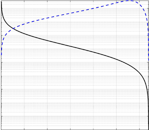
To see the effect of these dispersion coefficients, we study one of the test cases proposed by Kolehmainen et al. (Reference Kolehmainen, Ozel and Sundaresan2018). They studied a three-dimensional periodic box of  $192d_p \times 8d_p \times 8d_p$. Initially, the particles at
  $x<96d_p$ are charged positively
  $Q_p=Q_0$ and the particles at
  $x\geq 96d_p$ are charged negatively
  $Q_p=-Q_0$. An initial granular temperature is imposed, and it remains constant during the simulation. We also neglect all the external forces (gravity, drag, electrostatic, etc.). For simplicity, in this part we also neglect the triboconductivity effect; this is analysed in the next section. Using these hypotheses, the charge transport equation can be simplified to a one-dimensional diffusion equation
 \begin{equation} n_p \frac{\partial Q_p}{\partial t} = n_p[ D_p^{{coll}} + ( 1 + \eta_{{coll}} ) D_p^{{kin}} ] \frac{\partial^2 Q_p}{\partial x^2}. \end{equation}
This equation can be solved analytically
 \begin{gather} Q_p = \sum_{n=1}^{\infty} \lambda_n \exp({-(D_p^{{coll}} + ( 1 + \eta_{{coll}} ) D_p^{{kin}})( {2{\rm \pi} n}/{L})^2 t)} \sin\left( \frac{2{\rm \pi} n x}{L} \right) \end{gather}
 \begin{gather}\lambda_n = \frac{2Q_0}{n{\rm \pi}}( 1 - ( -1 )^n), \end{gather}
where  $L=192d_p$ is the box length in the
  $x$ direction.
This equation allows us to study the evolution of the electric charge as a function of time. For the simulation, we use the same type of particles as before and we set  $\alpha _p=0.60$. In figure 6 we plot the particle charge spatial profile for different values of the non-dimensional time
  $t^*=( {\sqrt {\varTheta }}/{d_p})t$. As we can see, the electric charge is dispersed inside the domain as the time passes and tends to reach the equilibrium value
  $Q_p=0$.

Figure 6. Particle charge profile as a function of  $x/L$ at different times
  $t^*=( {\sqrt {\varTheta }}/{d_p})t$.
A more interesting analysis can be performed if we separate the kinetic and collisional contributions to the dispersion mechanism. Figures 7, 8 and 9 show the particle charge profile for a dense system ( $\alpha _p=0.60$), a dilute system (
 $\alpha _p=0.05$) and an intermediate system (
 $\alpha _p=0.55$). The squares markers with a solid line represent the total dispersion, the solid line represents for the collisional contribution and the dashed line is the contribution of the kinetic term. As we can see, for dilute systems, the dispersion comes almost exclusively from the kinetic dispersion coefficient contribution. On the contrary, for dense systems, the collisional term accounts for most of the electric charge dispersion. However, we can see that, for intermediate values, both coefficients are of the same order of magnitude; they both need to be taken into account in order to accurately predict the dispersion phenomenon.

Figure 7. Particle charge profile at  $t^*=10\,000$ for
  $\alpha _p=0.60$.

Figure 8. Particle charge profile at  $t^*=200$ for
  $\alpha _p=0.05$.

Figure 9. Particle charge profile at  $t^*=20\,000$ for
  $\alpha _p=0.55$.
7. Triboconductivity effect
In addition to the dispersion phenomenon, we found that both the collision term (4.7) and the charge–velocity correlation (5.6) lead to electrical current density transport effects in the mean electric charge equation. These triboelectrical current density contributions obey separate mesoscopic Ohm's laws in terms of collisional and kinetic triboconductivity coefficients,  $\sigma _p^{{coll}}$ and
  $\sigma _p^{{kin}}$, respectively. In figure 10, we represent both contributions as a function of the solid volume fraction. For this particular type of particle, we can see that the kinetic contribution can be dropped for high values of
  $\alpha _p$.

Figure 10. Collisional and kinetic triboconductivity coefficient.
The charge transport equation (5.10) for this simplified problem is written
 \begin{align} n_p \frac{\partial Q_p}{\partial t} = -( \sigma_p^{{coll}} + ( 1 + \eta_{{coll}} ) \sigma_p^{{kin}}) \frac{\partial E}{\partial x} + \frac{\partial}{\partial x}\left[ n_p D_p^{{coll}} + n_p ( 1 + \eta_{{coll}} ) D_p^{{kin}} \frac{\partial Q_p}{\partial x} \right]. \end{align}
Now, taking the divergence of (2.5), we have
 \begin{equation} \frac{\partial E}{\partial x} = - \frac{\partial^2 \varphi}{\partial x^2}. \end{equation}
Using (2.4), and given that the medium permittivity is constant, we obtain
 \begin{equation} \frac{\partial E}{\partial x} = \frac{\varrho}{\varepsilon_0}, \end{equation}
where,  $\varrho = n_p Q_p$ is the volume charge density. Finally, the divergence of the electric field can be written as
 \begin{equation} \frac{\partial E}{\partial x} = \frac{n_pQ_p}{\varepsilon_0}. \end{equation}
This leads to a closed mean charge transport equation of the form
 \begin{align} n_p \frac{\partial Q_p}{\partial t} = -n_p\frac{\sigma_p^{{coll}} + \left( 1 + \eta_{{coll}} \right) \sigma_p^{{kin}}}{\varepsilon_0}Q_p + \frac{\partial}{\partial x}\left[ n_p D_p^{{coll}} + n_p \left( 1 + \eta_{{coll}} \right) D_p^{{kin}} \frac{\partial Q_p}{\partial x} \right]. \end{align}
If we apply this equation to the simplified problem described before, we find the analytic solution (7.6). Using the same parameters as before, we can determine the dynamic evolution of the electric charge (figure 11). As we can see, the electric charge reaches the equilibrium value faster, which confirms the fact that the triboconductivity helps the redistribution of the electric charge. However, it is worth noting that the triboconductivity effect seems to be more important than the dispersion process, this was also reported in the literature (Kolehmainen et al. Reference Kolehmainen, Ozel and Sundaresan2018).
 \begin{align} Q_p &=
\sum_{n=1}^{\infty} \lambda_n \exp([
-(({ \sigma_p^{{coll}} + ( 1 + \eta_{{coll}} ) \sigma_p^{{kin}}})/{
\varepsilon_0})\notag\\ &\quad - ( D_p^{{coll}}
+ ( 1 + \eta_{{coll}} ) D_p^{{kin}})
( {2{\rm \pi} n}/{L})^2 ] t)\sin\left(
\frac{2{\rm \pi} n x}{L} \right).
\end{align}
\begin{align} Q_p &=
\sum_{n=1}^{\infty} \lambda_n \exp([
-(({ \sigma_p^{{coll}} + ( 1 + \eta_{{coll}} ) \sigma_p^{{kin}}})/{
\varepsilon_0})\notag\\ &\quad - ( D_p^{{coll}}
+ ( 1 + \eta_{{coll}} ) D_p^{{kin}})
( {2{\rm \pi} n}/{L})^2 ] t)\sin\left(
\frac{2{\rm \pi} n x}{L} \right).
\end{align}
Figure 11. Particle charge profile as a function of  $x/L$ at different times
  $t^*=( {\sqrt {\varTheta }}/{d_p})t$.
In order to verify this, we rewrite the equation (7.5), so we make the characteristic times for the dispersion ( $\tau _D$) and the triboconductivity (
 $\tau _\sigma$) appear. Taking
  $l$ as the dispersion characteristic length, we have
 \begin{gather} \frac{\partial Q_p}{\partial t} = - \left( \left( 1 + \eta_{{coll}} \right) \frac{1}{\tau_\sigma^{{kin}}} + \frac{1}{\tau_\sigma^{{coll}}} \right)Q_p + l^2\left( \left( 1 + \eta_{{coll}} \right) \frac{1}{\tau_D^{{kin}}} + \frac{1}{\tau_D^{{coll}}} \right) \frac{\partial^2 Q_p}{\partial x^2}, \end{gather}
 \begin{gather}\tau_\sigma = \frac{\varepsilon_0}{\sigma_p}, \end{gather}
 \begin{gather}\tau_D = \frac{l^2}{D_p}. \end{gather}
 If we chose  $l=L$, then we can represent them as a function of the solid volume fraction (figure 12). We remark that the triboconductivity characteristic time is much smaller than the dispersion characteristic time for almost all values of
  $\alpha _p$. For dense regimes, where the collisional triboconductivity and dispersion coefficient are much larger than their kinetic counterparts, the ratio between these two characteristic times reduces to
 \begin{equation} \frac{\tau_\sigma^{{coll}}}{\tau_D^{{coll}}} \propto \left( \frac{d_p}{l} \right)^2. \end{equation}
Figure 12. Triboconductivity and dispersion characteristic times as a function of solid volume fraction for  $\varTheta =0.01\ \textrm {m}^{2}\,\textrm {s}^{-2}$.
This shows, that for dense systems, the dispersion effect is only comparable to the triboconductivity when the dispersion characteristic length scale is of the same order as the particle diameter.
8. Conclusions
In this work, we derived an Eulerian particle model for the mean electric charge equation in gas–solid flow using the framework provided by the kinetic theory of rapid granular flows. The transport equation for the mean electric charge was fully closed using less restrictive hypotheses than previous works found in the literature. The collision term in the transport equation was closed without assuming the electric charge probability density function explicitly. We proposed a linear model for the mean electric charge conditioned by the instantaneous particle velocity to account for the charge–velocity correlation. To close the charge–velocity correlation, we also derived the corresponding transport equation with the same set of hypotheses for the collision term modelling. Then, by using a series of additional hypotheses, we derived an algebraic model for the charge–velocity correlation from the corresponding transport equation. Finally, the modelled particle–particle collision term and electric charge–velocity correlation are considered in the electric charge transport equation, allowing us to identify their main effects. First of all, we found a charge dispersion phenomenon written as the sum of two separate contributions: a collisional contribution due to the electric charge transfer during particle–particle collisions and a kinetic contribution due to the transport of electric charge by the random motion of particles. Each contribution was written using separate gradient model approximations, leading us to derive an electric charge dispersion coefficient as the sum of two separate collisional and kinetic contributions. We showed that the collisional dispersion coefficient is predominant in dense regimes and that the kinetic dispersion coefficient is the most important in dilute ones. There is, nevertheless, an intermediate region where both coefficients have to be taken into account in order to accurately predict the dispersion effect. In addition to the dispersion phenomenon, we found than both the collision term and the charge–velocity correlation lead to electrical current density transport effects in the mean electric charge transport equation. These triboelectrical current density contributions obey separate mesoscopic Ohm's laws in terms of collisional and kinetic triboconductivity coefficients,  $\sigma _p^{{coll}}$ and
  $\sigma _p^{{kin}}$, respectively. Finally, in order to determine which is more important between the dispersion and the triboelectrical current effects, we derived their characteristic times. These parameters allowed us to show that, for dense regimes, both mechanisms are of the same order of magnitude if the characteristic dispersion length scale is comparable with the particle diameter. For dilute regimes, the analysis is more complicated and depends on the particle size and physical properties, the solid fraction and the particle agitation.
Acknowledgements
This work was supported by the ANR–IPAF project, grant ANR-16-CE06-0008 of the French National Agency of Research (ANR).
Declaration of interests
The authors report no conflict of interest.
Appendix A. Integral collision coefficients
The coefficients appearing in the collision terms (4.6) and (5.5) have the following numerical values:
 \begin{align*} \varUpsilon^{(1.1)}&=\frac{2^{{14}/{5}}5}{3 \times 7}\varGamma\left(\frac{3}{2}\right)\varGamma \left(\frac{12}{5}\right),\\ \varUpsilon^{(1.2)}&=\frac{2^{{14}/{5}}5}{3 \times 7}\varGamma\left(\frac{12}{5}\right)\varGamma \left(\frac{3}{2}\right),\\ \varUpsilon^{(1.3)}&=\frac{2^{{4}/{5}}}{{\rm \pi}^{2}}\varGamma\left(\frac{29}{10}\right)\varGamma \left(\frac{3}{2}\right),\\ \varUpsilon^{(1.4)}&=\frac{2^{{24}/{5}}5}{3\times 19}\varGamma\left(\frac{29}{10}\right)\varGamma \left(\frac{3}{2}\right),\\ \varUpsilon^{(1.5)}&=\frac{2^{{9}/{5}}}{{\rm \pi}^{2}}\varGamma\left(\frac{34}{10}\right) \varGamma\left(\frac{3}{2}\right),\\ \varUpsilon^{(2.1)}&=\frac{2^{3}}{3}\varGamma(3)\varGamma\left(\frac{3}{2}\right),\\ \varUpsilon^{(2.2)}&=\frac{2^{{24}/{5}}5}{3 \times 7}\varGamma \left(\frac{34}{10}\right)\varGamma\left(\frac{3}{2}\right),\\ \varUpsilon^{(2.3)}&=\frac{2^{{14}/{5}}5}{3 \times 19}\varGamma\left(\frac{29}{10}\right) \varGamma\left(\frac{3}{2}\right),\\ \varUpsilon^{(2.4)}&=\frac{2^{{14}/{5}}5}{3 \times 19}\varGamma\left(\frac{29}{10}\right) \varGamma\left(\frac{3}{2}\right),\\ \varUpsilon^{( 3.2 )} &= \frac{2^{{24}/{5}}5}{7}\varGamma \left( \frac{24}{10} \right)\varGamma \left(\frac{3}{2}\right),\\ \varUpsilon^{( \xi )} &= \frac{\varUpsilon^{( 2.4 )}}{\varUpsilon^{( 3.2 )}}, \end{align*}
where  $\varGamma$ is the gamma function.
Appendix B. Electric charge covariance transport equation
Following the mean general transport equation (3.12), we set  $\phi _p=\xi _{p}^{\prime }\xi _{p}^{\prime }$
 \begin{equation} n_{p}\frac{\textrm{D}\langle \xi_{p}^{\prime}\xi_{p}^{\prime}\rangle }{\textrm{D}t} +2n_{p}\langle \xi_{p}^{\prime}c_{p,i}^{\prime}\rangle \frac{\partial Q_{p}}{\partial x_{i}}+\frac{\partial}{\partial x_{i}}(n_{p}\langle \xi_{p}^{\prime}\xi_{p}^{\prime}c_{p,i}^{\prime}\rangle )=\mathcal{C}(\xi_{p}\xi_{p})-2Q_{p}\mathcal{C}(\xi_{p}), \end{equation}
 \begin{align} \mathcal{C}(\xi_{p}\xi_{p})&= d_{p}^{3}\beta E_{j}\frac{\partial Q_{p}}{\partial x_{j}} (\varTheta_{p})^{{9}/{10}}n_{p}^{2}g_{0}\varUpsilon^{(3.1)}\nonumber\\ &\quad -d_{p}^{2}\frac{\beta}{\gamma}\langle \xi_{p}^{\prime}\xi_{p}^{\prime} \rangle n_{p}^{2}g_{0}(\varTheta_{p})^{{9}/{10}}\varUpsilon^{(3.2)}\nonumber\\ &\quad - d_{p}^{2}\frac{\beta}{\gamma}Q_{p}^{2}n_{p}^{2}g_{0}(\varTheta_{p})^{{9}/{10}}\varUpsilon^{(3.2)}\nonumber\\ & \quad +d_{p}^{2}\beta^{2}E_{l}E_{j}n_{p}^{2}g_{0}(\varTheta_{p})^{{13}/{10}} \varUpsilon_{lj}^{(3.4)}\nonumber\\ &\quad -d_{p}^{2} E_{l}\frac{\beta^2}{\gamma}d_{p}\frac{\partial Q_{p}}{ \partial x_{j}}(\varTheta_{p})^{{13}/{10}}n_{p}^{2}g_{0} \varUpsilon_{lj}^{(3.5)}\nonumber\\ & \quad +d_{p}^{2} E_{l}\frac{\beta^2}{B}B_{s}(\varTheta_{p})^{{18}/{10}} n_{p}^{2}g_{0}\varUpsilon_{ls}^{(3.6)}\nonumber\\ &\quad +d_{p}^{2}\left(\frac{\beta}{\gamma}\right)^{2}Q_{p}B_{j} (\varTheta_{p})^{{18}/{10}}n_{p}^{2}g_{0}\varUpsilon_{j}^{(3.7)}\nonumber\\ &\quad -\frac{\partial}{\partial x_{i}}(-d_{p}^{3}\beta E_{i}Q_{p}n_{p}^{2} (\varTheta_{p})^{{9}/{10}}g_{0}\varUpsilon^{(3.8)})\nonumber\\ &\quad +\frac{\partial}{\partial x_{i}}\left(d_{p}^{3}\left(\frac{\beta}{\gamma}\right)^{2} Q_{p}B_{j}(\varTheta_{p})^{{18}/{10}}g_{0}n_{p}^{2} \varUpsilon_{ij}^{(3.9)}\right). \end{align}
Therefore, we can identify a destruction term of the electric charge covariance due to particle–particle interactions
 \begin{equation} n_{p}\frac{\partial\langle \xi_{p}^{\prime}\xi_{p}^{\prime}\rangle }{\partial t}+ \cdots=-n_{p}\frac{1}{\tau_{\xi}}\langle \xi_{p}^{\prime}\xi_{p}^{\prime}\rangle +\cdots, \end{equation}
where  $\tau _{\xi }$ is the characteristic time of electric charge covariance destruction by collisions
 \begin{equation} \tau_{\xi}=\left( \varUpsilon^{( 3.2 )} d_p^2 \frac{\beta}{\gamma}n_pg_0\varTheta_p^{{9}/{10}}\right)^{-1}. \end{equation}
With
 \begin{equation} \varUpsilon^{( 3.2)} = \frac{2^{{24}/{5}} 5}{7}\varGamma \left( \frac{24}{10} \right)\varGamma \left( \frac{3}{2} \right). \end{equation}


