


1. Introduction
The purpose of this study is to construct a model based on the Poisson–Nernst–Planck and Stokes equations in the thin Debye layer limit for the flow and deformation of an inclusion that is embedded in an exterior medium, where both the inclusion and exterior medium are electrolyte solutions. The flow and deformation are driven by an imposed electric field and the solutions are strong electrolytes. Two examples are considered side by side. In one example, the electrolyte solutions and their solvents are immiscible, so that the inclusion is a drop, and the interface between the two fluids is assumed to be completely impervious to the passage of ions, so that it is referred to as ideally polarisable. This is perhaps the simplest model for the interface between two immiscible electrolyte solutions (ITIES) of electrochemistry. In the other example, the same electrolyte solution occupies both the interior and exterior phases, which are separated by an interfacial membrane, such as an inextensible lipid bilayer or a vesicle membrane. The membrane significantly impedes the passage of both solvent and ions but still allows a small flux of each species to pass separately between the two phases.
At each point of the interface the diffuse charge Debye layers on its opposite sides have opposite polarity, and together the pair are referred to as an electrical double layer. Both the Debye layer and double layer are fundamental concepts in electrochemistry and colloid science, and have been studied theoretically since Helmholtz (Reference Helmholtz1853), often in the context of an electrically charged solid in contact with an electrolyte solution. The underlying structure used here for the distribution of ions and the electrostatic potential within each Debye layer is the Gouy–Chapman model, due to Gouy (Reference Gouy1910) and Chapman (Reference Chapman1913), in which diffusion of ions is balanced by an electrostatic Coulomb force acting on their electrical charge at the continuum level. Although the model has been developed since to include additional effects such as the non-zero size of ions, the influence of the solvation shell around an ion and other realistic effects, these developments all retain the basic constituents of the Gouy–Chapman model at their core. The texts by Russel, Saville & Schowalter (Reference Russel, Saville and Schowalter1989) and Hunter (Reference Hunter2001) give a review of the general theory of the Debye and double layer and describe related experiments.
The mechanism for flow and deformation is as follows. The electric field  $\boldsymbol {E}$ in the medium causes ions to move or migrate under the action of an electrostatic Coulomb force, with the (positively charged) cations moving in the direction of
  $\boldsymbol {E}$ and the (negatively charged) anions moving in the direction opposite to
  $\boldsymbol {E}$. Both ion species are advected with the underlying fluid velocity modified by a molecular drift velocity due to the combined effects of a concentration-dependent diffusive flux and the Coulomb-force-induced electromigration. Away from boundaries and interfaces that impede their motion ions are present in number densities according to their valence that maintain zero net charge or electroneutrality. For simplicity we consider binary symmetric electrolytes with valence 1 ions, so that these number densities are equal.
However, near a boundary or interface that stops or impedes the movement of ions in the normal direction, ion densities change and charge separation occurs. Positive charge develops when  $\boldsymbol {E}$ has a normal component directed from the medium to the interface and negative charge develops when
  $\boldsymbol {E}$ has a normal component in the opposite direction, that is, directed from the interface into the medium. An electrical double layer forms, with Debye layers of opposite polarity on either side of the interface.
The presence of separated or induced charge in a net electric field causes a force to be exerted on the fluid locally. The force has a normal component that can deform the interface and a tangential component that induces fluid flow along the interface with accompanying shear stress that can also cause interfacial motion and deformation. This is an example, for a deformable interface, of induced charge electrokinetic flow, or induced charge electro-osmosis (ICEO). It is described by Russel et al. (Reference Russel, Saville and Schowalter1989) and Hunter (Reference Hunter2001), and more recent reviews of the theory and experiments of ICEO have been given by, for example, Squires & Bazant (Reference Squires and Bazant2004) and Bazant & Squires (Reference Bazant and Squires2010). Girault (Reference Girault2010) reviewed the electrochemistry of liquid–liquid interfaces, i.e. ITIES, and Reymond et al. (Reference Reymond, Fermin, Lee and Girault2000) discussed current and potential applications at their time of writing.
Much of the recent interest in electrokinetic flow and the related area of electrohydrodynamics (EHD) is motivated by their applications in microfluidics; Vlahovska (Reference Vlahovska2019) gives a comprehensive review that addresses fundamental aspects of many studies in EHD. Central to electrohydrodynamics is the leaky dielectric model of Melcher & Taylor (Reference Melcher and Taylor1969), and a contrast between electrohydrodynamics and electrokinetics is described in the introduction of the review by Saville (Reference Saville1997). Namely, in EHD electric charge is situated at or on the interface between media of different electric permittivity that are either weakly polarisable or weak conductors of charge due to the relatively low concentration of ions that is typical of the solution of a weak electrolyte. The influence of a diffuse charge cloud is either small or absent, and charge accumulates at the interface via conservation of current and mild ohmic conductivity in the bulk phase. Large electric field strengths, of the order of kilovolts per centimetre, must be applied to induce a flow under these circumstances. On the other hand, in electrokinetics, charge-carrying ions are plentiful and present in a diffuse charge cloud near a surface. The action of the applied field on this induced charge cloud dominates the dynamics, and an applied field of the order of a few volts per centimetre is often sufficient to induce flow. Here, the abundance of ions is typical of an aqueous solution of a strong electrolyte at a comparable molarity.
The focus of the study by Saville (Reference Saville1997) was a derivation of the leaky dielectric model based on the Poisson–Nernst–Planck equations of electrokinetics that is applicable to poorly conducting liquids. In this sense, he explains, the two topics merge. Further, this had been anticipated by Taylor (Reference Taylor1966) in the concluding remarks of his study on the circulation induced in a drop by an electric field. There he comments that the predictions of the electrohydrodynamic model ‘may be expected to be realistic even if the charge is not exactly situated at the interface, provided its distance from the interface is small compared with the linear scale of the situation’.
Since Saville (Reference Saville1997), two more recent studies on the derivation of the leaky dielectric, electrohydrodynamic model as a limiting form of the Poisson–Nernst–Planck equations have been made by Schnitzer & Yariv (Reference Schnitzer and Yariv2015) and by Mori & Young (Reference Mori and Young2018). In § 10.2 a comparison is made between these two studies and the present one. However, we note here that the main differences are: (i) the present study is in the electrokinetic regime, not the electrohydrodynamic regime; (ii) the velocity scale here is  $U_{*c}=D_{*}/\lambda _{*}$ associated with diffusion of charge across a Debye layer, where
  $D_{*}$ is an ion diffusion constant and
  $\lambda _{*}$ is the Debye layer screening length. The associated time scale
  $\tau _{*c}=\lambda _{*} a_{*}/D_{*}$, where
  $a_{*}$ is the inclusion length scale, is that on which the separated charge in a Debye layer changes in response to a change in strength of the externally applied field. This is substantially faster that the time scale associated with the Helmholtz–Smoluchowski slip velocity of studies in electrohydrodynamics.
Pascall & Squires (Reference Pascall and Squires2011) gave a detailed study of electrokinetic phenomena at liquid–liquid interfaces. Their main focus is the dependence of the free-stream or slip velocity of an electrolyte solution, far from a double layer, on characteristic properties of the underlying media. In particular, given an imposed tangential electric field, there is an increase in the free-stream velocity by a factor of  $d_{*}/\lambda _{*}\gg 1$ if a liquid film of thickness
  $d_{*}$ is introduced between the electrolyte solution and an underlying solid metal substrate. This occurs when the liquid film is either a perfect conductor or a dielectric permeated by an electric field. Their study compares and successfully reconciles the results and predictions of earlier studies, and establishes similar results for the electrophoresis of spherical liquid drops. The geometry is fixed, either planar or spherical, and the context is that of a steady state.
The present study is organised as follows. In § 2 the governing field equations and boundary conditions, including the conditions at a drop and vesicle interface, are stated together with initial conditions and far-field conditions for an imposed electric field. The field equations consist of the Poisson–Nernst–Planck equations coupled to the equations of zero-Reynolds-number or Stokes flow. Non-dimensional scales are introduced and the non-dimensional form of the system is given in § 2.4. The Nernst–Planck equations for the ion concentrations include rate terms that express the rate of dissociation of salt or electrolyte into ions and the recombination or association of ions into salt. In § 3 the limit of a strong electrolyte is formed, for which all or nearly all of the dissolved salt is present in its dissociated form as ions. The analysis then proceeds with the ion concentration equations in an effectively rate-free form.
In the thin Debye layer limit, a representative Debye layer thickness  $\lambda _{*}$ is much less than the linear dimension
  $a_{*}$ of the inclusion, so that their ratio
  $\epsilon =\lambda _{*}/a_{*}$ is small, that is,
  $0<\epsilon \ll 1$. The
  $\epsilon \rightarrow 0$ limit is taken up first in § 4, where the field equations that apply in the outer regions, away from the Debye layers, are given at leading order in an
  $\epsilon$ expansion. These equations are devoid of source or inhomogeneous forcing terms.
Section 5 concerns the structure of the inner regions or Debye layers. A surface-fitted intrinsic coordinate system is introduced (§ 5.1). With this, the Gouy–Chapman solution for the ion concentrations and electrostatic potential within the layers is constructed, at leading order, in a form that is parameterised by variables at the outer edges of the Debye layers (§ 5.2). Expressions for the pressure and fluid velocity in terms of the local or excess potential within the layers are given in § 5.4, with a similar parameterisation.
For two immiscible electrolyte solutions, a drop possesses a charged double layer even when in equilibrium, and the accompanying jump in potential across the double layer is referred to as an inner or Galvani potential (Hunter Reference Hunter2001). This potential, via the Debye layer  $\zeta$-potentials, is expressed in terms of ion partition coefficients in the reduced or small-
 $\epsilon$ limit in § 5.3. In § 5.5 reduced expressions are given for the small but non-zero trans-membrane ion flux and osmotic solvent flux across a vesicle membrane.
To form a closed, reduced asymptotic or macro-scale model it is necessary to consider the transport of ions within the Debye layers, which is the subject of § 6. Sections 6.1 and 6.2 give the transport relations that are specific to a drop and to a vesicle, and their use as interfacial boundary conditions is taken up in § 6.3.
In § 7 a Fredholm second kind integral equation is derived that gives the fluid velocity on the interface in terms of a net interfacial traction and an integral term that depends on the electrostatic energy density contained in the double layer and which has a Stokes-dipole kernel. Some details of the construction are given in Appendix A. Section 8 recalls the integral equation for the electrostatic potential.
A formulation via integral equations is convenient for simulating large-amplitude deformations. For small-amplitude deformation the stress-balance boundary condition at the interface can be used instead, and this, expressed in terms of quantities at the outer edges of the Debye layers and known surface data, is given in Appendix B for a drop and for a vesicle. The location in the text of relations that are needed to form the model is summarised in § 9. Section 10 contains sample solutions for the flow about a drop, together with a brief comparison between the present electrokinetic model and derivations of the Taylor–Melcher electrohydrodynamic model given by Schnitzer & Yariv (Reference Schnitzer and Yariv2015) and by Mori & Young (Reference Mori and Young2018). Concluding remarks are made in § 11.
2. Formulation: governing equations and boundary conditions
The formulation begins with the Nernst–Planck equations for a dilute electrolyte solution coupled to the Stokes equation for an incompressible fluid. For a symmetric one-to-one binary electrolyte, with one positive ion species (or cation) of charge  $e$ and one negative ion species (or anion) of the same valency, the Nernst–Planck equations for ion conservation are
 $$\begin{gather} \partial_t c^{({\pm})} + \boldsymbol{\nabla}\boldsymbol{\cdot} (c^{({\pm})}\boldsymbol{v}^{({\pm})})={\mathcal{R}} , \end{gather}$$
 $$\begin{gather}\boldsymbol{v}^{({\pm})} - \boldsymbol{u} ={\mp} b^{({\pm})}e\boldsymbol{\nabla}\phi - D^{({\pm})}\boldsymbol{\nabla} \ln c^{({\pm})} , \end{gather}$$
with conservation of the combined salt given by
 $$\begin{gather} \partial_t s + \boldsymbol{\nabla}\boldsymbol{\cdot} (s\boldsymbol{v})={-} {\mathcal{R}} , \end{gather}$$
 $$\begin{gather}\boldsymbol{v} - \boldsymbol{u} ={-} D_{s}\boldsymbol{\nabla} \ln s . \end{gather}$$
Quantities specific to an ion species are given a  $(\pm )$ superscript to denote the ion charge,
  $(+)$ for the cation and
  $(-)$ for the anion, and
  $c$ denotes the ion species concentration. The Eulerian velocity of a species is denoted by
  $\boldsymbol {v}$ and the mass averaged fluid velocity is
  $\boldsymbol {u}$.
Equation (2.1b) gives the drift velocity of ions through the fluid. This is due to (i) the Coulomb force on ion charges in the electric field, which induces electromigration, with ion mobility  $b^{(\pm )}$ and electrostatic potential
  $\phi$, and (ii) the diffusion of ions due to variations in their concentration, with ion diffusivity given by the Einstein–Smoluchowski relation
  $D^{(\pm )}=b^{(\pm )}k_{B}T$. The drift velocity is also the product of the ion mobility and the net thermodynamic force acting on the ions, which is minus the gradient of their electrochemical potential, and (2.1b) is referred to as the Nernst–Planck relation (Russel et al. Reference Russel, Saville and Schowalter1989). It can be used to recast the expression for the molecular ion flux, which is
 \begin{equation} \boldsymbol{j}^{({\pm})}=c^{({\pm})}(\boldsymbol{v}^{({\pm})} - \boldsymbol{u}) . \end{equation}
The concentration of the electrically neutral, combined salt is denoted by  $s$, with diffusivity
  $D_{s}$. The rate term
  ${\mathcal {R}}$ is given by
 \begin{equation} {\mathcal{R}}= k_{d}s -k_{a} c^{(+)}c^{(-)} , \end{equation}
where  $k_{d}$ is the rate of dissociation of the salt into ions and
  $k_{a}$ is the rate of association of ions into salt.
A subscript is used to denote separate phases,  $\varOmega _{in}$ for the dispersed or interior phase and
  $\varOmega _{ex}$ for the continuous or exterior phase. Later, the same convention for subscripts will be applied to material parameters and ambient species concentrations, which can be different in the two phases but are constant within each phase. However, it will be omitted initially when the distinction does not need to be made.
The electric displacement  $\boldsymbol {D}$, electric field
  $\boldsymbol {E}$ and volumetric charge density
  $\rho$ satisfy the relations
 \begin{equation} \boldsymbol{\nabla}\boldsymbol{\cdot} \boldsymbol{D}=\rho, \quad \boldsymbol{D}=\varepsilon \boldsymbol{E}, \quad \boldsymbol{E}={-}\boldsymbol{\nabla} \phi, \quad \rho=e(c^{(+)}-c^{(-)}) . \end{equation}
These are Gauss's law, a linear constitutive relation with relative electric permittivity or dielectric constant  $\varepsilon$, the relation between the electric field and the electrostatic potential and the charge density in terms of the ion densities, respectively. Together they give the Poisson equation in the form
 \begin{equation} \nabla^{2}\phi={-}\frac{e}{\varepsilon}(c^{(+)}-c^{(-)}). \end{equation}
In the Stokes flow or zero-Reynolds-number limit for incompressible solutions,
 \begin{equation} \boldsymbol{\nabla} \boldsymbol{\cdot} \boldsymbol{u}=0\quad \mbox{and} \quad -\boldsymbol{\nabla} p +\mu{\nabla}^{2}\boldsymbol{u} + \rho \boldsymbol{E} = 0 , \end{equation}
where  $p$ is the pressure. The Coulomb force term
  $\rho \boldsymbol {E}$ in the Stokes equation provides the coupling from the electrostatic field or Nernst–Planck and Poisson equations to the fluid field, and can be expressed in various equivalent ways by use of (2.5a–d).
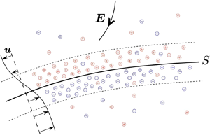
A sketch of the Debye layer pair near the interface which introduces some of the notation that we use is given in figure 1.

Figure 1. An interior phase  $\varOmega _{in}$ with boundary
  $\partial \varOmega _{in}$ and an exterior phase
  $\varOmega _{ex}$ with boundary
  $\partial \varOmega _{ex}$ are separated by the interface
  $S$ of a drop or a vesicle membrane that is either impervious or nearly impervious to the passage of ions. An electric field with strength
  $\boldsymbol {E}$ induces a flow of ions that charges up a pair of Debye layers of opposite polarity. The outer edges of the Debye layers are denoted by
  $S_{+}$ in the exterior phase and
  $S_{-}$ in the interior phase and the induced flow velocity of the host solvent is denoted by
  $\boldsymbol {u}$.
2.1. Boundary conditions for a drop
In the boundary conditions adopted for a drop, the interface has no electrical capacitance and no monopole surface charge. It is also impervious or impenetrable to ions, and is therefore referred to as ideally polarisable. This gives the interfacial boundary conditions
 \begin{equation} [\phi]=0, \quad [\boldsymbol{D}\boldsymbol{\cdot}\boldsymbol{n}]=0, \quad \mbox{and} \quad \boldsymbol{j}^{({\pm})} \boldsymbol{\cdot}\boldsymbol{n}=0 \quad \mbox{on} \ S , \end{equation}
respectively. Here  $S$ denotes the sharp interface between the two phases, with outward unit normal
  $\boldsymbol {n}$, and
  $[\,\cdot\, ]\equiv [\,\cdot\, ]^{\partial \varOmega _{ex}}_{\partial \varOmega _{in}}$ denotes the jump across
  $S$, with the convention that it is the limit as
  $S$ is approached from the exterior domain
  $\varOmega _{ex}$ minus the limit as
  $S$ is approached from the interior domain
  $\varOmega _{in}$.
Continuity of velocity of the solvent and the kinematic boundary condition imply that
 \begin{equation} [\boldsymbol{u}]=0 \quad \mbox{and} \quad \left(\boldsymbol{u}-\frac{\partial\boldsymbol{x}_{s}}{\partial t}\right)\boldsymbol{\cdot}\boldsymbol{n}=0 \quad \mbox{on} \ S, \end{equation}
where  $\boldsymbol {x}_{s}$ is any point on
  $S$. The stress-balance boundary condition is that
 \begin{equation} [(\boldsymbol{\mathsf{T}}_{H} + \boldsymbol{\mathsf{T}}_{M})\boldsymbol{\cdot}\boldsymbol{n}] = \sigma(\kappa_{1}+\kappa_{2})\boldsymbol{n} \quad \mbox{on} \ S,\end{equation}
where
 \begin{equation} \boldsymbol{\mathsf{T}}_{H}={-}p\boldsymbol{\mathsf{I}}+2\mu\boldsymbol{\mathsf{e}} \quad \mbox{and} \quad \boldsymbol{\mathsf{T}}_{M}= \varepsilon\big(\boldsymbol{\nabla} \phi \otimes \boldsymbol{\nabla} \phi-\tfrac{1}{2}|\boldsymbol{\nabla}\phi|^{2}\boldsymbol{\mathsf{I}}\big) . \end{equation}
Here  $\boldsymbol{\mathsf{T}}_{H}$ is the stress tensor for a Newtonian fluid with viscosity
  $\mu$ and
  $(\boldsymbol {e})_{ij}=(\partial _{x_{j}}u_{i}+\partial _{x_{i}}u_{j})/2$ is the symmetric part of the velocity gradient. We use
  $\boldsymbol{\mathsf{T}}_{M}$ to denote the part of the Maxwell stress tensor due to the electric field, which has been written in terms of the potential
  $\phi$,
  $\sigma$ is a constant surface tension and
  $\kappa _{1}$ and
  $\kappa _{2}$ are the principal curvatures of
  $S$. With
  $\boldsymbol {n}$ pointing outward on
  $S$, the principal curvatures are taken to be positive when the curve of intersection of
  $S$ by a plane containing
  $\boldsymbol {n}$ and a principal direction is convex on the side to which
  $\boldsymbol {n}$ points, and is negative otherwise.
Under equilibrium conditions there is typically a difference in the electric potential between distinct phases that occurs at and near the interface between them. It is caused by a difference in the affinity for charge carriers of the phases and is referred to as an inner or Galvani potential (Hunter Reference Hunter2001). The boundary conditions
 \begin{equation} c^{(+)}|_{\partial\varOmega_{in}} = l^{(+)} c^{(+)}|_{\partial\varOmega_{ex}} \quad \mbox{and} \quad c^{(-)}|_{\partial\varOmega_{in}} = l^{(-)} c^{(-)}|_{\partial\varOmega_{ex}} \quad \mbox{on} \ S , \end{equation}
where  $l^{(+)}$ and
  $l^{(-)}$ are constant partition coefficients, imply the presence of a non-zero Galvani potential when
  $l^{(+)}\neq l^{(-)}$. The notation
  $c^{(\pm )}|_{\partial \varOmega _{in,ex}}$ denotes evaluation of the ion concentration
  $c^{(\pm )}$ in the limit as
  $S$ is approached from the interior domain
  $\varOmega _{in}$ or exterior domain
  $\varOmega _{ex}$. Boundary conditions of this type have been considered by, for example, Zholkovskij, Masliyah & Czarnecki (Reference Zholkovskij, Masliyah and Czarnecki2002) and by Mori & Young (Reference Mori and Young2018).
2.2. Boundary conditions for a cell or vesicle
Mori, Liu & Eisenberg (Reference Mori, Liu and Eisenberg2011) introduce a set of phenomenological boundary conditions for the behaviour of a cell or vesicle, where the interior and exterior phases are separated by a membrane, and these are summarised here. Similar boundary conditions for a membrane have been considered by Lacoste et al. (Reference Lacoste, Menon, Bazant and Joanny2009). The membrane is treated as a sharp interface  $S$ between the phases that nonetheless has electromechanical structure. Its initial equilibrium reference configuration, denoted by
  $S_{ref}$, has a Lagrangian or material point coordinate system
  $\boldsymbol {\theta }$, and at later times its position is described by
  $\boldsymbol {x}=\boldsymbol {X}(\boldsymbol {\theta }, t)$.
The same notation for interfacial quantities is used for both a drop and a vesicle. Here we have:  $[\,\cdot\, ]$ for the jump in a quantity across the membrane,
  $\cdot |_{\partial \varOmega _{in,ex}}$ for evaluation as the side
  $\partial \varOmega _{in,ex}$ of the membrane is approached or simply on
  $S$ for a quantity that is continuous.
If the membrane is semi-permeable or porous to the aqueous solvent it allows a flow of solvent in the normal direction that occurs by osmosis and is assumed to be proportional to the jump in the solvent's partial pressure across the membrane. Hence,
 \begin{equation} \boldsymbol{u}-\left.\frac{\partial\boldsymbol{X}}{\partial t}\right|_{\boldsymbol{\theta}} ={-} {\rm \pi}_{m} \, [ p- k_{B}T (c^{(+)}+c^{(-)}) ] \, \boldsymbol{n} \quad \mbox{on} \ S , \end{equation}
where  ${\rm \pi} _{m} \geqslant 0$ is an effective membrane porosity and the partial pressure of the ions is given by the ideal gas law.
The trans-membrane flux for each ion species is taken to be proportional to the jump in its electrochemical potential across the membrane surface. Mori et al. (Reference Mori, Liu and Eisenberg2011) give the boundary condition
 \begin{equation} c^{({\pm})} \left(\boldsymbol{v}^{({\pm})} - \left.\frac{\partial\boldsymbol{X}}{\partial t}\right|_{\boldsymbol{\theta}}\right) \boldsymbol{\cdot} \boldsymbol{n} ={-} g^{({\pm})} [ k_{B}T \ln c^{({\pm})} \pm e \phi ] \quad \mbox{on} \ S , \end{equation}
where  $g^{(\pm )}\geqslant 0$ is a gating constant for each ion species, and the velocity on the left-hand side,
  $\boldsymbol {v}^{(\pm )}-\partial _{t}\boldsymbol {X}|_{\boldsymbol {\theta }}$, is the velocity of ions relative to the membrane material.
In the analysis that follows, a boundary condition is needed for the normal component of the molecular ion flux  $\boldsymbol {j}^{(\pm )}\boldsymbol {\cdot }\boldsymbol {n}$ in the electrolyte solution immediately adjacent to the membrane, where the flux
  $\boldsymbol {j}^{(\pm )}$ is given by (2.3), i.e.
  $\boldsymbol {j}^{(\pm )}=c^{(\pm )}(\boldsymbol {v}^{(\pm )} - \boldsymbol {u})$. If the normal ion flux
  $\boldsymbol {j}^{(\pm )}\boldsymbol {\cdot }\boldsymbol {n}$ in the electrolyte and the normal ion flux across the membrane given by (2.14) are not equal, then charge is not conserved at the membrane boundaries
  $\partial \varOmega _{in,ex}$ but accumulates there. We note that this occurs if both (2.13) and (2.14) are applied to a membrane that is semi-permeable to solvent, i.e. when
  ${\rm \pi} _{m} > 0$. This is verified by subtracting (2.13) multiplied by the ion concentration
  $c^{(\pm )}$ from (2.14) to form the electrolyte ion flux
  $\boldsymbol {j}^{(\pm )}\boldsymbol {\cdot }\boldsymbol {n}$, and noting that the concentration of each ion species is not continuous but has a jump across the membrane.
This difficulty is easily resolved by modifying the trans-membrane flux boundary condition (2.14) to read
 \begin{equation} c^{({\pm})} (\boldsymbol{v}^{({\pm})} - \boldsymbol{u}) \boldsymbol{\cdot} \boldsymbol{n} ={-} g^{({\pm})} [ k_{B}T \ln c^{({\pm})} \pm e \phi ] \quad \mbox{on} \ S , \end{equation}
which conserves charge across the membrane and its boundaries and holds in general, that is, for all  ${\rm \pi} _{m} \geqslant 0$. When the membrane is impermeable to solvent (i.e.
  ${\rm \pi} _{m}=0$) the boundary condition (2.13) reduces to no-slip between the electrolyte and membrane surface, and (2.14) and (2.15) are identical, but when the membrane is semi-permeable to solvent (i.e.
  ${\rm \pi} _{m} > 0$), the solvent and ion species cross the membrane at different rates via distinct pores or channels, and (2.15) must be applied instead.
The membrane has electrical capacitance because it can maintain a jump in the potential across its outer faces, between which the potential varies linearly with normal distance. The jump in the potential is referred to as the trans-membrane potential and is denoted by  $[\phi ]$. The membrane has no net monopole charge, in the sense that at distinct points along the normal the surface charge densities on opposite faces have equal magnitude and opposite polarity, cancelling each other. The charge on each face is related to the trans-membrane potential by the membrane capacitance per unit area
  $C_{m}$. Analogous to the first two boundary conditions of (2.8) for a drop, but modified to express continuity of electric displacement and the capacitance of the membrane, we have the vesicle boundary conditions
 \begin{equation} \varepsilon \boldsymbol{\nabla} \phi\boldsymbol{\cdot}\boldsymbol{n}|_{\partial\varOmega_{in}} = \varepsilon \boldsymbol{\nabla} \phi\boldsymbol{\cdot}\boldsymbol{n}|_{\partial\varOmega_{ex}} = C_{m} [\phi] \quad \mbox{where} \ C_{m} =\frac{\varepsilon_{m}}{d} . \end{equation}
Here  $\varepsilon _{m}$ is the membrane permittivity and
  $d$ is its thickness.
Two specific membrane capacitance models of Mori et al. (Reference Mori, Liu and Eisenberg2011) are
 \begin{equation} C_{m} =
\left\{\begin{array}{@{}ll} C_{m}^{0} & (a) , \\
C_{m}^{0}
\delta A (\boldsymbol{X}) & (b) . \end{array} \right.
\end{equation}
\begin{equation} C_{m} =
\left\{\begin{array}{@{}ll} C_{m}^{0} & (a) , \\
C_{m}^{0}
\delta A (\boldsymbol{X}) & (b) . \end{array} \right.
\end{equation}
These hold if, for example, the bulk material of the membrane is incompressible, and then (2.17a) applies when the membrane surface is locally inextensible and (2.17b) applies when it is locally extensible. The capacitance per unit area in the initial undeformed or reference state is  $C_{m}^{0}$, which is constant for a homogeneous membrane. The ratio of the local surface area in the deformed state to its value in the initial reference state following a material point
  $\boldsymbol {x}=\boldsymbol {X}(\boldsymbol {\theta }, t)$ is denoted by
  $\delta A (\boldsymbol {X})$. Bulk incompressibility implies that the volume of a membrane material element
  ${d}(\boldsymbol {X}) \delta A (\boldsymbol {X})$ is conserved during deformation, so that for the locally inextensible surface of (2.17a)
  $\delta A (\boldsymbol {X})=1$ with
  ${d}(\boldsymbol {X})$ and
  $C_{m}^{0}$ conserved, whereas for (2.17b)
  ${d}(\boldsymbol {X})^{-1} \propto \delta A (\boldsymbol {X})$.
The stress-balance boundary condition is
 \begin{align} [(\boldsymbol{\mathsf{T}}_{H} + \boldsymbol{\mathsf{T}}_{M})\boldsymbol{\cdot}\boldsymbol{n}] = 2\sigma H \boldsymbol{n} - \boldsymbol{\nabla}_{s} \sigma - \kappa_{b} \left( (2H-C_{0})\left(H^{2}-K+\frac{C_{0}H}{2}\right) + {\nabla}_{s}^{2} H \right) \boldsymbol{n} \end{align}
on  $S$. The vesicle membrane has a bending stiffness that is expressed in terms of the bending modulus
  $\kappa _{b}$, the mean curvature
  $H=(\kappa _{1}+\kappa _{2})/2$, the Gaussian curvature
  $K=\kappa _{1}\kappa _{2}$ and a spontaneous curvature
  $C_{0}$. The spontaneous curvature
  $C_{0}$ is twice the mean curvature of the membrane material in a traction-free equilibrium state, see, for example, Vlahovska, Podgorski & Misbah (Reference Vlahovska, Podgorski and Misbah2009) and Seifert (Reference Seifert1999), and it is usually set to zero. Here,
  $\boldsymbol {\nabla }_{s}$ denotes the surface gradient operator,
  ${\nabla }_{s}^{2}$ is the Laplace–Beltrami or surface Laplacian operator and the convention for the sign of the principal curvatures
  $\kappa _{1}$ and
  $\kappa _{2}$ is the same as that in (2.10).
The tension in the membrane surface is denoted by  $\sigma$ in (2.18), but, in contrast to its appearance in (2.10) for a drop, the value of
  $\sigma$ is not a given constant. For a locally inextensible membrane
  $\sigma$ is determined by imposing inextensibility as a constraint, namely
 \begin{equation} \boldsymbol{\nabla}_{s}\boldsymbol{\cdot}\left( \frac{\partial}{\partial t} \boldsymbol{X}_{s}(\boldsymbol{\theta}, t)\right) =0 , \end{equation}
or, equivalently,  $\delta A (\boldsymbol {X})=1$, for all
  $t>0$. Here
  $\partial _{t}\boldsymbol {X}_{s}$ denotes the tangential projection of the velocity
  $\partial _{t}\boldsymbol {X}$ of a material particle onto
  $S$. For a locally extensible membrane a stress–strain equation of state must be introduced, see, for example, Barthès-Biesel (Reference Barthès-Biesel2011). The membrane tension is initially constant, but during deformation it can vary from point to point on
  $S$, leading to the term
  $\boldsymbol {\nabla }_{s} \sigma$ in (2.18).
We note that Mori et al. (Reference Mori, Liu and Eisenberg2011) considered a membrane bending stress given by the variational derivative of a general energy functional. The specific choice of the functional due to Helfrich (Reference Helfrich1973) has been adopted in many studies of cell and vesicle deformation, and leads to the bending stress term on the right-hand side of (2.18). Barthès-Biesel (Reference Barthès-Biesel2011) gives a concise description of the different mechanical properties of vesicle, cell and capsule membranes.
2.3. The far-field and initial conditions
The electric field that induces flow and deformation is applied at time  $t=0$. It can be spatially uniform and constant, or more general, so that
 \begin{equation}
\boldsymbol{E}\rightarrow \left\{ \begin{array}{@{}ll}
E_{\infty}\boldsymbol{e}_{z} & \mbox{for a uniform field}
\\ -\boldsymbol{\nabla} \phi_{\infty} & \mbox{in general}
\end{array} \right.\quad \mbox{as} \ |\boldsymbol{x}|
\rightarrow \infty \ \mbox{for} \ t > 0,
\end{equation}
\begin{equation}
\boldsymbol{E}\rightarrow \left\{ \begin{array}{@{}ll}
E_{\infty}\boldsymbol{e}_{z} & \mbox{for a uniform field}
\\ -\boldsymbol{\nabla} \phi_{\infty} & \mbox{in general}
\end{array} \right.\quad \mbox{as} \ |\boldsymbol{x}|
\rightarrow \infty \ \mbox{for} \ t > 0,
\end{equation}
where  $\phi _{\infty }$ is a solution of Laplace's equation. In addition,
 \begin{equation} \boldsymbol{u}(\boldsymbol{x}, t) \rightarrow 0 \quad \mbox{and} \quad c^{({\pm})}(\boldsymbol{x}, t) \rightarrow \ \mbox{const. as}\ |\boldsymbol{x}|\rightarrow \infty \ \mbox{for} \ t > 0 . \end{equation}
 A drop is assumed to have relaxed to a spherical shape for  $t<0$, with no applied field and equilibrium initial conditions given by
 \begin{equation} \boldsymbol{u}(\boldsymbol{x}, 0)=0 \quad \mbox{and} \quad c^{({\pm})}(\boldsymbol{x}, 0)= \mbox{piecewise constant for all}\ \boldsymbol{x} . \end{equation}
However, when there is a non-zero Galvani potential difference between the two phases the  $t<0$ equilibrium relations for the potential and ion concentrations are revised to accommodate an electrical double layer; this is considered later, in § 5.3.
2.4. Non-dimensionalisation
Quantities used to put the equations in non-dimensional form are listed in table 1. The length scale  $a_{*}$ is the initial drop radius, or a similar length scale for a vesicle. The velocity scale
  $U_{*c}=D_{*}/\lambda _{*}$ is the ion-diffusive scale, where
  $D_{*}$ is a representative ion diffusivity and
  $\lambda _{*}$ is the Debye layer screening thickness. The time scale
  $\tau _{*c}=a_{*}/U_{*c}$ is the scale on which charge in the Debye layers changes in response to changes in the applied electric field, i.e. the charge-up time scale. The scale for the pressure
  $p$ is the scale of the Stokes flow regime, and the scale for the potential is the thermal voltage
  $k_{B}T/e$, where
  $k_{B}$ is the Boltzmann constant and
  $T$ is the temperature.
Table 1. Variables are made non-dimensional by the quantities shown.

All material and rate parameters in the two phases are made non-dimensional by a single representative value. For example, the ion concentrations are made non-dimensional by a representative ambient ion concentration  $c_{*}$, and the salt concentration is made non-dimensional by
  $s_{*}$. Similarly,
  $D^{(\pm )}, k_{d}, k_{a}, \varepsilon$,
  $\sigma$ and
  $\mu$ are made non-dimensional by
  $D_{*}, k_{d*}, k_{a*}, \varepsilon _{*}$,
  $\sigma _{*}$ and
  $\mu _{*}$, respectively. To observe equilibrium between the ion and salt concentrations, the relation
 \begin{equation} k_{d*}s_{*}=k_{a*}c_{*}^{2} \end{equation}
holds. The Debye layer thickness  $\lambda _{*}$ is given by
 \begin{equation} \lambda_{*}^{2}=\frac{\varepsilon_{*}k_{B}T}{2c_{*}e^{2}} . \end{equation}
Dimensionless groups that appear are
 $$\begin{gather} \tau=\frac{k_{d*}a_{*}}{U_{*c}} \gg 1, \quad \alpha= \frac{c_{*}}{s_{*}} \gg 1, \quad \epsilon=\frac{\lambda_{*}}{a_{*}} \ll 1, \end{gather}$$
 $$\begin{gather}\varDelta=\frac{\sigma_{*}}{\mu_{*}U_{*c}}, \quad \nu=\frac{\varepsilon_{*}(k_{B}T/e)^{2}}{\mu_{*}D_{*}} \quad \mbox{and} \quad \varPsi = \frac{e\varPhi_{*\infty}}{k_{B}T} . \end{gather}$$
The role of  $\tau$ and
  $\alpha$ is considered in the following, in § 3. Except for this, the analysis is carried out in the limit of small Debye layer thickness,
  $\epsilon \rightarrow 0$, with
  $\varDelta$,
  $\nu$ and
  $\varPsi$ all of order
  $O(1)$. The quantity
  $\varDelta$ is the ratio of the capillary velocity
  $\sigma _{*}/\mu _{*}$ to the ion-diffusive velocity
  $U_{*c}$. The group
  $\nu \epsilon$ is the ratio of electrostatic stress to viscous stress, and is sometimes referred to either as the inverse of a Mason number or as an electrical Hartmann number. If the Helmholtz–Smoluchowski slip velocity
  $U_{*HS}$ is based on the thermal voltage, then
  $U_{*HS}=\varepsilon _{*}(k_{B}T/e)^{2}/\mu _{*}a_{*}$, and the group
  $\nu \epsilon = U_{*HS}/U_{*c}$ is also the ratio of the two velocity scales. The parameters
  $\epsilon$,
  $\varDelta$ and
  $\nu$ are all fixed for a given choice of electrolytes and initial inclusion size. In contrast, the parameter
  $\varPsi$ is the ratio of the change in potential difference
  $\varPhi _{*\infty } = E_{*\infty }a_{*}$ on the inclusion length scale to the thermal voltage, and is a control parameter.
In the scaling regime of this study, the Péclet number  $Pe=U_{*c}a_{*}/D_{*}$ does not appear independently, because the velocity scale for
  $U_{*c}$ implies that
  $Pe=\epsilon ^{-1}$.
The same variable and parameter names are now used to express the governing equations and boundary conditions in non-dimensional form. The molecular ion flux  $\boldsymbol {j}^{(\pm )}=c^{(\pm )}(\boldsymbol {v}^{(\pm )} - \boldsymbol {u})$ of (2.3), recast via (2.1b) and the relation
  $D^{(\pm )}=b^{(\pm )}k_{B}T$, is
 \begin{equation} \boldsymbol{j}^{({\pm})} ={-} \epsilon D^{({\pm})}( \boldsymbol{\nabla} c^{({\pm})} \pm c^{({\pm})}\boldsymbol{\nabla} \phi ) , \end{equation}
in non-dimensional form. Conservation of ions (2.1) and salt (2.2), together with the expression (2.4) for the ion kinetic rate term  $\mathcal {R}$ and the incompressibility condition of (2.7a,b) give
 $$\begin{gather} (\partial_{t}+\boldsymbol{u}\boldsymbol{\cdot}\boldsymbol{\nabla})c^{({\pm})}-\epsilon D^{({\pm})}\boldsymbol{\nabla}\boldsymbol{\cdot} ( \boldsymbol{\nabla} c^{({\pm})}\pm c^{({\pm})}\boldsymbol{\nabla} \phi) = \tau \alpha^{{-}1} (k_{d}s-k_{a}c^{(+)}c^{(-)}) , \end{gather}$$
 $$\begin{gather}(\partial_{t}+\boldsymbol{u}\boldsymbol{\cdot}\boldsymbol{\nabla})s-\epsilon D_{s}\nabla^{2} s ={-} \tau (k_{d}s-k_{a}c^{(+)}c^{(-)}) . \end{gather}$$
The Poisson equation (2.6) is
 \begin{equation} \epsilon^{2}\nabla^{2}\phi={-}\frac{q}{\varepsilon} , \quad \mbox{where}\ q = \frac{c^{(+)}-c^{(-)}}{2} , \end{equation}
so that  $q$ is a normalised charge density. The continuity and Stokes equation are
 \begin{equation} \boldsymbol{\nabla} \boldsymbol{\cdot} \boldsymbol{u}=0\quad \mbox{and} \quad -\boldsymbol{\nabla} p + \mu {\nabla}^{2}\boldsymbol{u} + \varepsilon \nu \epsilon \nabla^{2}\phi\boldsymbol{\nabla}\phi = 0 , \end{equation}
where the body force is written in terms of the potential via (2.5a–d).
2.4.1 Drop boundary conditions
In non-dimensional form, from (2.5a–d) and (2.26), the interfacial boundary conditions (2.8) on  $S$ become
 \begin{equation} [\phi]=0, \quad [\varepsilon \boldsymbol{\nabla} \phi\boldsymbol{\cdot}\boldsymbol{n}] = 0 , \end{equation}
and
 \begin{equation} \boldsymbol{j}^{({\pm})} \boldsymbol{\cdot}\boldsymbol{n}=0 , \quad \mbox{or equivalently} \ ( \boldsymbol{\nabla} c^{({\pm})}\pm c^{({\pm})}\boldsymbol{\nabla} \phi)\boldsymbol{\cdot} \boldsymbol{n}=0 . \end{equation}
Continuity of velocity and the kinematic condition are formally unchanged, namely
 \begin{equation} [\boldsymbol{u}]=0 \quad \mbox{and} \quad \left(\boldsymbol{u} - \frac{\partial\boldsymbol{x}_{s}}{\partial t}\right)\boldsymbol{\cdot}\boldsymbol{n}=0 \quad \mbox{on} \ S . \end{equation}
The stress-balance boundary condition becomes
 \begin{equation} [(\boldsymbol{\mathsf{T}}_{H} + \nu\epsilon\boldsymbol{\mathsf{T}}_{M})\boldsymbol{\cdot}\boldsymbol{n}] = \varDelta(\kappa_{1}+\kappa_{2})\boldsymbol{n} \quad \mbox{on} \ S,\end{equation}
where
 \begin{equation} \boldsymbol{\mathsf{T}}_{H}={-}p\boldsymbol{\mathsf{I}}+2 \mu \boldsymbol{\mathsf{e}} \quad \mbox{and} \quad \boldsymbol{\mathsf{T}}_{M}= \varepsilon \big(\boldsymbol{\nabla} \phi \otimes \boldsymbol{\nabla} \phi-\tfrac{1}{2}|\boldsymbol{\nabla}\phi|^{2}\boldsymbol{\mathsf{I}}\big) . \end{equation}
The boundary conditions (2.12) for a Galvani potential (when  $l^{(+)}\neq l^{(-)}$) are formally unchanged, namely
 \begin{equation} c^{(+)}|_{\partial\varOmega_{in}} = l^{(+)} c^{(+)}|_{\partial\varOmega_{ex}} \quad \mbox{and} \quad c^{(-)}|_{\partial\varOmega_{in}} = l^{(-)} c^{(-)}|_{\partial\varOmega_{ex}} \quad \mbox{on} \ S . \end{equation}
2.4.2 Vesicle boundary conditions
In non-dimensional form, the trans-membrane ion flux  $\boldsymbol {j}^{(\pm )} \boldsymbol {\cdot }\boldsymbol {n}$ is given by
 \begin{equation} c^{({\pm})} (\boldsymbol{v}^{({\pm})}-\boldsymbol{u}) \boldsymbol{\cdot} \boldsymbol{n} ={-} \epsilon g^{({\pm})} [ \ln c^{({\pm})} \pm \phi ] \quad \mbox{on} \ S , \end{equation}
where the gating constant  $g^{(\pm )}$ of (2.15) has been made non-dimensional and scaled by
  $g_{*}={c_{*}D_{*}}/{k_{B}Ta_{*}}$. The flow of solvent across the membrane is given by
 \begin{equation} \boldsymbol{u} - \left.\frac{\partial\boldsymbol{X}}{\partial t}\right|_{\boldsymbol{\theta}} ={-} \epsilon {\rm \pi}_{m} \left[ \frac{2\epsilon}{\nu} p - (c^{(+)}+c^{(-)}) \right] \boldsymbol{n} \quad \mbox{on} \ S , \end{equation}
where the effective porosity  ${\rm \pi} _{m}$ of (2.13) has been made non-dimensional and scaled by
  ${\rm \pi} _{*}={D_{*}}/{k_{B}Tc_{*}a_{*}}$. These relations contrast with the boundary conditions (2.32) and (2.33) for an ideally polarisable drop with a sharp impervious interface; the cell has a small
  $O(\epsilon )$ flux of ions and solvent across the membrane when it is semi-permeable to these species.
The relations (2.16) that express continuity of electric displacement across the membrane become
 \begin{equation} \varepsilon \epsilon \boldsymbol{\nabla} \phi\boldsymbol{\cdot}\boldsymbol{n}|_{\partial\varOmega_{in}} = \varepsilon \epsilon \boldsymbol{\nabla} \phi\boldsymbol{\cdot}\boldsymbol{n}|_{\partial \varOmega_{ex}} = C_{m} [\phi] . \end{equation}
As a lipid bilayer or similar biomembrane has a thickness of the order of  $5$–
$5$– $8$ nm, which is the same order of magnitude as the thickness of the neighbouring Debye layers, the membrane thickness has been made non-dimensional by
  $\lambda _{*}$ and the membrane capacitance per unit area,
  $C_{m}$ or
  $C_{m}^{0}$ of (2.17), has been made non-dimensional by
  $\varepsilon _{*}/\lambda _{*}$. This accounts for the
  $\epsilon$-scaling in (2.39).
The stress-balance boundary condition is now
 \begin{equation} [(\boldsymbol{\mathsf{T}}_{H} + \nu \epsilon \boldsymbol{\mathsf{T}}_{M})\boldsymbol{\cdot}\boldsymbol{n}] = 2 \sigma H \boldsymbol{n} - \boldsymbol{\nabla}_{s} \sigma - \kappa_{b} (2H(H^{2}-K) + {\nabla}_{s}^{2} H ) \boldsymbol{n} , \end{equation}
where the tension in the membrane and the bending modulus have been made non-dimensional by  $\mu _{*}U_{*c}$ and
  $\mu _{*}U_{*c}a_{*}^{2}$ respectively, and the spontaneous curvature
  $C_{0}$ has been set to zero. The membrane inextensibility constraint is formally unchanged, namely
 \begin{equation} \boldsymbol{\nabla}_{s}\cdot\left( \frac{\partial}{\partial t}\boldsymbol{X}_{s}(\boldsymbol{\theta}, t) \right) =0 . \end{equation}
2.4.3 Initial and far-field conditions
The initial conditions are
 \begin{equation} \phi(\boldsymbol{x}, 0^{+}) ={-} \varPsi z, \quad \boldsymbol{u}(\boldsymbol{x}, 0) = 0 \quad \mbox{and} \quad c^{({\pm})}(\boldsymbol{x}, 0) = c_{in,ex} \quad \mbox{on} \ \varOmega_{in,ex} , \end{equation}
except that the first and third relations are revised for a drop when it has a non-zero Galvani potential, as considered in § 5.3. Here  $c_{in}$ and
  $c_{ex}$ are the initial dimensionless ion concentrations on
  $\varOmega _{in}$ and
  $\varOmega _{ex}$, respectively. A drop is initially spherical with radius 1, whereas a vesicle has a known initial equilibrium configuration
  $S_{ref}$. Far from the inclusion, for a uniform applied field
 \begin{equation} \phi(\boldsymbol{x}, t) \sim{-} \varPsi z, \quad \boldsymbol{u}(\boldsymbol{x}, t) \rightarrow 0, \quad \mbox{and} \quad c^{({\pm})}(\boldsymbol{x}, t)\rightarrow c_{ex} \ \mbox{as} \ |\boldsymbol{x}|\rightarrow \infty \ \mbox{for} \ t > 0 . \end{equation}
For a more general applied field  $\phi$ approaches a specified solution
  $\phi _{\infty }$ of Laplace's equation that has magnitude
  $\varPsi$.
3. The strong electrolyte limit
The two dimensionless groups  $\tau$ and
  $\alpha$ that multiply the rate term
  $\mathcal {R}$ on the right-hand side of (2.27) and (2.28) are defined at (2.25a). Of these,
  $\tau =k_{d*}a_{*}/U_{*c}$ is the ratio of the dissociation rate of salt to the rate of Debye layer charge-up, which is taken to be large. The group
  $\alpha =c_{*}/s_{*}$ is the ratio of the ambient concentration of the dissociated ions to that of the combined salt, which is large for a strong electrolyte.
In the limit  $\tau \rightarrow \infty$, (2.28) implies that to leading order
 \begin{equation} k_{d}s-k_{a} c^{(+)}c^{(-)}=0 , \end{equation}
that is, for all  $\boldsymbol {x}$ and
  $t$ the ion and salt concentrations are in equilibrium at leading order throughout both phases. The right-hand side of the ion conservation equation (2.27) is now of order
  $\tau /\alpha$ times a residual rate term that is of order
  $o(1)$. Provided
  $\tau /\alpha$ is bounded, that is, provided
  $\alpha \rightarrow \infty$ as fast as or faster than
  $\tau \rightarrow \infty$, the right-hand side of (2.27) is
  $o(1)$, which is sufficiently small for it to be neglected as a higher-order effect in the small-
 $\epsilon$ analysis that is developed in the following.
The conservation equations (2.27) and (2.28) can now be simplified: the  $o(1)$ right-hand side rate term of (2.27) for the ion concentrations
  $c^{(+)}$ and
  $c^{(-)}$ is omitted, and after the ion concentrations have been found the leading-order salt concentration
  $s$ is given by (3.1), if required. Equation (2.28) for conservation of
  $s$ can then be omitted, because it contains no further information at the order of calculation of the model. Instead of (2.27) and (2.28), we have
 \begin{equation} (\partial_{t}+\boldsymbol{u}\boldsymbol{\cdot}\boldsymbol{\nabla})c^{({\pm})}-\epsilon D^{({\pm})}\boldsymbol{\nabla}\boldsymbol{\cdot} ( \boldsymbol{\nabla} c^{({\pm})}\pm c^{({\pm})}\boldsymbol{\nabla} \phi) = 0 . \end{equation}
 An equation for the conservation of charge  $q$ is given by forming the difference of (3.2) for the ion species, or by forming the difference of (2.27), to give
 \begin{align} (\partial_{t}+\boldsymbol{u}\boldsymbol{\cdot}\boldsymbol{\nabla}) q = \frac{\epsilon}{2} ( D^{(+)}\nabla^{2}c^{(+)} - D^{(-)}\nabla^{2}c^{(-)} + D^{(+)}\boldsymbol{\nabla}\boldsymbol{\cdot} (c^{(+)}\boldsymbol{\nabla} \phi) + D^{(-)}\boldsymbol{\nabla}\boldsymbol{\cdot} (c^{(-)}\boldsymbol{\nabla} \phi) ) \end{align}
which is exact. The terms grouped on the right-hand side represent charge diffusion.
4. The outer regions away from the Debye layers
In the outer regions, away from the Debye layers, the dependent variables are expanded in integer powers of  $\epsilon$, so that for the ion concentrations and potential, respectively
 $$\begin{gather} c^{({\pm})}=c_{0}^{({\pm})}+\epsilon c_{1}^{({\pm})}+\cdots , \end{gather}$$
 $$\begin{gather}\phi=\phi_{0}+\epsilon \phi_{1}+\cdots , \end{gather}$$
with analogous notation for expansions of  $\boldsymbol {u}$,
  $p$ and
  $q$.
$q$.
To a high degree of approximation, the outer regions are charge neutral and the electrostatic body force in the momentum equation is zero. To see this, note that the Poisson equation (2.29) implies that in an outer approximation  $q_{0} = q_{1}=0$, so that
 \begin{equation} c_{0}^{(+)}=c_{0}^{(-)} \quad \mbox{and} \quad c_{1}^{(+)}=c_{1}^{(-)} \end{equation}
for all  $\boldsymbol {x}$ and
  $t$. Then, at leading order the ion conservation equations (3.2) imply that
 \begin{equation} (\partial_{t}+\boldsymbol{u}_{0}\boldsymbol{\cdot}\boldsymbol{\nabla})c_{0}^{({\pm})}=0 , \end{equation}
so that throughout the outer regions, from the first of relations (4.2a,b),
 \begin{equation} (\partial_{t}+\boldsymbol{u}_{0}\boldsymbol{\cdot}\boldsymbol{\nabla})c_{0} = 0 , \end{equation}
where
 \begin{equation} c_{0}^{(+)} = c_{0}^{(-)} \stackrel{\mathrm{def}}{=} c_{0} \ \mbox{is conserved on particle paths} \frac{{\rm d}\boldsymbol{x}}{{\rm d}t}=\boldsymbol{u}_{0} . \end{equation}
As the two ion concentrations are equal, the indication of their charge has been omitted.
The outer regions of  $\varOmega _{in}$ and
  $\varOmega _{ex}$ are partitioned into subdomains. An outflow subdomain consists of fluid that, at any time
  $t\geqslant 0$, originates from or exits a Debye layer. For want of better terminology, we refer to its complement, which is non-empty at least for sufficiently early times, as an inflow subdomain. Note that if the flow in the outer regions continually recirculates, an inflow subdomain can vanish at some time. However, at the outer edges of the Debye layers, there are always outflow regions where fluid exits the layer to enter the bulk and complementary inflow regions where fluid enters the layer from the bulk. The inflow and outflow subdomains are three-dimensional volumes, whereas the inflow and outflow regions are surfaces.
Figure 2 gives an illustrative sketch of outflow and inflow regions neighbouring the interface. They are distinguished by the sign of the quantity  $\partial _{n}v_{p}|_{S}$, which is introduced in § 5.4 and is the rate of extension (for
  $\partial _{n}v_{p}|_{S}>0$) or contraction (for
  $\partial _{n}v_{p}|_{S}<0$) of a Lagrangian fluid line element that is normal to the interface.

Figure 2. Sketch of characteristics or particle paths  $\boldsymbol {x}$ such that
  ${{\rm d}\kern0.06em \boldsymbol {x}}/{{\rm d}t}=\boldsymbol {u_{0}}$ showing inflow and outflow regions for the Debye layer in the exterior domain
  $\varOmega _{ex}$. The inflow and outflow regions are separated by the location of the marker (
 $\bullet$), which is such that
  $\partial _{n}v_{p}|_{S}=0$ as explained in § 5.4. An impression is given of the deformation of a Lagrangian fluid volume as it enters and leaves the Debye layer. The counterpart in
  $\varOmega _{in}$ is not shown.
On the inflow subdomains, at sufficiently early times the initial and far-field conditions (2.42) and (2.43) imply that (4.4b) becomes
 \begin{equation} c_{0} = c_{in} \quad \mbox{and} \quad c_{0} = c_{ex} , \end{equation}
where  $c_{in}$ and
  $c_{ex}$ are the respective uniform initial ion concentrations on
  $\varOmega _{in}$ and
  $\varOmega _{ex}$. As
  $q_{1}=0$, (3.3) for charge conservation at order
  $O(\epsilon )$ implies that
  $\nabla ^{2}\phi _{0}=0$. From this, the Poisson equation (2.29) implies that
  $q_{2}=0$ also, and the result of charge neutrality at higher integer powers of
  $\epsilon$ begins to repeat or bootstrap: because
  $\nabla ^{2}\phi _{0}=0$ and
  $c_{0}^{(\pm )}$ is constant, ion conservation given by (3.2) at order
  $O(\epsilon )$ implies that
  $(\partial _{t}+\boldsymbol {u}_{0}\boldsymbol {\cdot }\boldsymbol {\nabla })c_{1}^{(\pm )}=0$. The second of relations (4.2a,b) with the far-field and initial conditions implies that
  $c_{1}^{(+)}$ and
  $c_{1}^{(-)}$ are equal and constant on each inflow subdomain. This constant would usually be set to zero, but in any event, because
  $q_{2}=0$ (3.3) for charge conservation at order
  $O(\epsilon ^{2})$ now implies that
  $\nabla ^{2}\phi _{1}=0$, etc.
On the outflow subdomains relations (4.2a,b) to (4.4b) still hold, but the initial data for the transport equation (4.3) is given by matching to the ion concentrations on outflow from the evolving Debye layers. In contrast to (4.5a,b),  $c_{0}$ is then a function of
  $\boldsymbol {x}$ and
  $t$ in the Eulerian frame. Similarly, if regions of re-entrant flow develop, when fluid re-enters a Debye layer it carries a value of
  $c_{0}(\boldsymbol {x}, t)$ equal to the ion concentration that it held at its previous exit. As
  $q_{1}=0$, (3.3) for conservation of charge at order
  $O(\epsilon )$ now implies a constraint or consistency condition between the ion concentration
  $c_{0}$ and the potential
  $\phi _{0}$, which is
 \begin{equation} (D^{(+)}-D^{(-)})\nabla^{2}c_{0} + (D^{(+)}+D^{(-)}) \boldsymbol{\nabla} \boldsymbol{\cdot} (c_{0} \boldsymbol{\nabla} \phi_{0} ) = 0 . \end{equation}
 Without formal proof, we assume that  $q_{2}=0$ everywhere, so that from (2.29) the potential satisfies the Laplace equation
 \begin{equation} \nabla^{2}\phi_{0}=0 \end{equation}
throughout the outer domains. It follows that the equations of Stokes flow are also unforced in the outer domains. That is,
 \begin{equation} \boldsymbol{\nabla} \boldsymbol{\cdot} \boldsymbol{u}_{0}=0 \quad \mbox{and} \quad -\boldsymbol{\nabla} p_{0} + \mu {\nabla}^{2}\boldsymbol{u}_{0} = 0 . \end{equation}
5. The Debye layers: equilibrium solution and hydrodynamics
5.1. The intrinsic coordinate system
To resolve the dynamics of the Debye layers, we introduce a local surface-fitted or intrinsic orthogonal curvilinear coordinate system. This has tangential coordinates  $\xi _{1}$ and
  $\xi _{2}$ that are aligned with the principal directions on
  $S$ and normal coordinate
  $n$, with
  $n=0$ on
  $S$ and
  $n>0$ in
  $\varOmega _{ex}$. The origins of the Eulerian and intrinsic coordinate systems are
  $O$ and
  $O^{\prime }$, respectively, and the position vector
  $\boldsymbol {x}$ of a point
  $P$ in space relative to
  $O$ is written in the two coordinate systems as
 \begin{equation} \boldsymbol{x}=\boldsymbol{X}(\xi_{1}, \xi_{2}, t) + n \boldsymbol{n}(\xi_{1}, \xi_{2}, t). \end{equation}
Here  $\boldsymbol {x}=\boldsymbol {X}(\xi _{1}, \xi _{2}, t)$ is the parametric equation of
  $S$ and
  $\boldsymbol {n}$ is its outward unit normal. As
  $\xi _{1}$ and
  $\xi _{2}$ are principal directions on
  $S$ they define (locally) an orthogonal coordinate system on it with associated unit tangent vectors
  $\boldsymbol {e}_{i}=({1}/{a_{i}})({\partial \boldsymbol {X}}/{\partial \xi _{i}})$, where
  $a_{i}=|{\partial \boldsymbol {X}}/{\partial \xi _{i}}|$ for
  $i=1, 2$. With the convention that
  $\boldsymbol {n}=\boldsymbol {e}_{1}\times \boldsymbol {e}_{2}$, Rodrigues’ formula implies that the principal curvatures
  $\kappa _{i}$ satisfy
  ${\partial \boldsymbol {n}}/{\partial \xi _{i}}=\kappa _{i}({\partial \boldsymbol {X}}/{\partial \xi _{i}})$, and the change in
  $\boldsymbol {x}$ corresponding to increments in the intrinsic coordinates with time fixed is
 \begin{equation} {\rm d}\boldsymbol{x}=l_{1}\,{\rm d}\xi_{1}\, \boldsymbol{e}_{1}+l_{2}\,{\rm d}\xi_{2}\, \boldsymbol{e}_{2}+{\rm d}n \, \boldsymbol{n}, \quad \mbox{where} \ l_{i}=a_{i}(1+n\kappa_{i}) \quad (i=1, 2). \end{equation}
Expressions for vector differential operators and the rate of strain tensor in a general orthogonal curvilinear coordinate system can be found in, for example, Batchelor (Reference Batchelor2000, Appendix 2).
Dependent variables within the Debye layers are denoted by uppercase letters, with terms in an expansion in integer powers of  $\epsilon$ denoted by subscripts, so that for the ion concentrations
  $c^{(\pm )}=C^{(\pm )}=C_{0}^{(\pm )}+\epsilon C_{1}^{(\pm )}+\cdots$ and for the potential
  $\phi =\varPhi = \varPhi _{0}+\epsilon \varPhi _{1}+\cdots$, for example. The analysis of the Debye layers is based on a local normal coordinate
  $N$ defined by
 \begin{equation} n=\epsilon N , \end{equation}
where  $N=O(1)$ as
  $\epsilon \rightarrow 0$.
5.2. The Gouy–Chapman solution
The leading-order ion concentrations and potential are given by the Gouy–Chapman solution. Reviews of this are given by, for example, Russel et al. (Reference Russel, Saville and Schowalter1989) and Hunter (Reference Hunter2001), and it is summarised here because it is the foundation for the analysis that follows. In the present context, all dependent variables depend parametrically on the tangential coordinates  $\xi _{1}$ and
  $\xi _{2}$, and on time
  $t$.
$t$.
In terms of local variables, at leading order, the ion conservation equations (3.2) and the interface condition (2.32) for a drop, or (2.37) with (2.26) for a vesicle, imply that
 $$\begin{gather} \partial_{N} (\partial_{N}C_{0}^{({\pm})}\pm C_{0}^{({\pm})}\partial_{N}\varPhi_{0})=0 \quad N \neq 0, \end{gather}$$
 $$\begin{gather}\mbox{with} \quad \partial_{N}C_{0}^{({\pm})}\pm C_{0}^{({\pm})}\partial_{N}\varPhi_{0} =0 \quad \mbox{on} \ S . \end{gather}$$
An integration immediately gives
 \begin{equation} \partial_{N}C_{0}^{({\pm})}\pm C_{0}^{({\pm})}\partial_{N}\varPhi_{0} =0 \quad \mbox{for all} \ N . \end{equation}
This has a simple interpretation in terms of the molecular ion flux (2.26), which has local expansion  $\boldsymbol {j}^{(\pm )}=\boldsymbol {J}_{0}^{(\pm )}+\epsilon \boldsymbol {J}_{1}^{(\pm )} + O(\epsilon ^{2})$ in the Debye layers, and where the leading-order flux
  $\boldsymbol {J}_{0}^{(\pm )}$ is in the normal direction. Equation (5.5) states that
  $\boldsymbol {J}_{0}^{(\pm )}$ is zero throughout the layers, with diffusion and electromigration of ions in equilibrium at this level of approximation.
The requirement of matching with the outer regions is that
 \begin{equation}
C_{0}^{({\pm})} \rightarrow
\left\{\begin{array}{@{}ll} c_{0}|_{S_{+}} & \mbox{as} \
N\rightarrow \infty \\ c_{0}|_{S_{-}} & \mbox{as} \
N\rightarrow -\infty \end{array} \right.\quad \mbox{and}
\quad \varPhi_{0}\rightarrow \left\{\begin{array}{@{}ll}
\phi_{0}|_{S_{+}} & \mbox{as} \ N\rightarrow \infty \\
\phi_{0}|_{S_{-}} & \mbox{as} \ N\rightarrow -\infty
\end{array} \right. , \end{equation}
\begin{equation}
C_{0}^{({\pm})} \rightarrow
\left\{\begin{array}{@{}ll} c_{0}|_{S_{+}} & \mbox{as} \
N\rightarrow \infty \\ c_{0}|_{S_{-}} & \mbox{as} \
N\rightarrow -\infty \end{array} \right.\quad \mbox{and}
\quad \varPhi_{0}\rightarrow \left\{\begin{array}{@{}ll}
\phi_{0}|_{S_{+}} & \mbox{as} \ N\rightarrow \infty \\
\phi_{0}|_{S_{-}} & \mbox{as} \ N\rightarrow -\infty
\end{array} \right. , \end{equation}
where an  $S_{+}$ or
  $S_{-}$ subscript denotes, respectively, the limit of a quantity in the outer regions as
  $S$ is approached from the exterior of the drop (as
  $n\rightarrow 0^{+}$) or from the interior (as
  $n\rightarrow 0^{-}$). We have just shown at (4.5a,b) that
  $c_{0}|_{S_{+}}=c_{ex}$ and
  $c_{0}|_{S_{-}}=c_{in}$ are constant over regions where the flow enters the Debye layers, at least at early times, but are to be determined and satisfy (4.4b) elsewhere.
Integration of (5.5) with the matching conditions (5.6a,b) gives the Boltzmann distribution between the ion concentrations and the potential, namely
 \begin{equation} C_{0}^{(+)}=c_{0}|_{S_{{\pm}}}e^{-\eta_{0}} , \quad C_{0}^{(-)}=c_{0}|_{S_{{\pm}}}e^{\eta_{0}} , \\ \end{equation}
where
 \begin{equation} \eta_{0}=
\left\{\begin{array}{@{}ll} \varPhi_{0}-\phi_{0}|_{S_{+}} &
\mbox{for} \ N>0, \\ \varPhi_{0}-\phi_{0}|_{S_{-}}
& \mbox{for} \ N<0. \end{array} \right.
\end{equation}
\begin{equation} \eta_{0}=
\left\{\begin{array}{@{}ll} \varPhi_{0}-\phi_{0}|_{S_{+}} &
\mbox{for} \ N>0, \\ \varPhi_{0}-\phi_{0}|_{S_{-}}
& \mbox{for} \ N<0. \end{array} \right.
\end{equation}
Here  $\eta _{0}$ is the first term in the expansion for
  $\eta =\varPhi -\phi |_{S_{\pm }}$, which is the excess potential in the Debye layers.
From (2.29), the charge density  $q$ in the layers is therefore given at leading order by
  $Q_{0}=-c_{0}|_{S_{\pm }}\sinh \eta _{0}$, and the potential
  $\varPhi _{0}$ satisfies the Poisson–Boltzmann equation
 \begin{equation} \varepsilon\partial_{N}^{2}\varPhi_{0}= c_{0}|_{S_{{\pm}}} \sinh (\varPhi_{0}-\phi_{0}|_{S_{{\pm}}}). \end{equation}
This can be integrated once on multiplying by  $\partial _{N}\varPhi _{0}$ and using the matching conditions (5.6a,b) to find
 \begin{equation} \varepsilon (\partial_{N}\varPhi_{0})^{2}=2 c_{0}|_{S_{{\pm}}} (\cosh (\varPhi_{0}-\phi_{0}|_{S_{{\pm}}})-1) . \end{equation}
For a drop, the first of the interfacial boundary conditions (2.31a,b), that  $[\phi ]=0$, states that the potential is continuous across
  $S$ with a surface value denoted by
  $\lim _{N\rightarrow 0^{\pm }}\varPhi _{0}=\varPhi _{0}|_{S}$. A second integration then gives the Gouy–Chapman solution in the form
 \begin{equation} \tanh \tfrac{1}{4}(\varPhi_{0}-\phi_{0}|_{S_{{\pm}}}) = \tanh \tfrac{1}{4} (\varPhi_{0}|_{S}-\phi_{0}|_{S_{{\pm}}}) \exp\left({{\mp}\sqrt{( c_{0}|_{S_{{\pm}}}/\varepsilon )} N}\right), \end{equation}
where the upper choice of signs hold for  $N>0$ and the lower choice for
  $N<0$. For a vesicle, its membrane capacitance implies that there can be a non-zero jump in the potential across the vesicle membrane, with
  $\lim _{N\rightarrow 0^{-}}\varPhi _{0} \equiv \varPhi _{0}|_{\partial \varOmega _{in}} \neq \lim _{N\rightarrow 0^{+}}\varPhi _{0} \equiv \varPhi _{0}|_{\partial \varOmega _{ex}}$. This gives the Gouy–Chapman solution
 $$\begin{gather} \tanh
\tfrac{1}{4}(\varPhi_{0}-\phi_{0}|_{S_{+}}) = \tanh
\tfrac{1}{4}
(\varPhi_{0}|_{\partial\varOmega_{ex}}-\phi_{0}|_{S_{+}})
\exp\left({- \sqrt{( c_{0}|_{S_{+}}/\varepsilon )} N}\right)\quad
\mbox{for} \ N>0 ,
\end{gather}$$
$$\begin{gather} \tanh
\tfrac{1}{4}(\varPhi_{0}-\phi_{0}|_{S_{+}}) = \tanh
\tfrac{1}{4}
(\varPhi_{0}|_{\partial\varOmega_{ex}}-\phi_{0}|_{S_{+}})
\exp\left({- \sqrt{( c_{0}|_{S_{+}}/\varepsilon )} N}\right)\quad
\mbox{for} \ N>0 ,
\end{gather}$$
 $$\begin{gather}\tanh
\tfrac{1}{4}(\varPhi_{0}-\phi_{0}|_{S_{-}}) = \tanh
\tfrac{1}{4}
(\varPhi_{0}|_{\partial\varOmega_{in}}-\phi_{0}|_{S_{-}})
\exp\left({ \sqrt{( c_{0}|_{S_{-}}/\varepsilon )} N}\right) \quad
\mbox{for} \ N <0 .
\end{gather}$$
$$\begin{gather}\tanh
\tfrac{1}{4}(\varPhi_{0}-\phi_{0}|_{S_{-}}) = \tanh
\tfrac{1}{4}
(\varPhi_{0}|_{\partial\varOmega_{in}}-\phi_{0}|_{S_{-}})
\exp\left({ \sqrt{( c_{0}|_{S_{-}}/\varepsilon )} N}\right) \quad
\mbox{for} \ N <0 .
\end{gather}$$
With the same convention for the choice of signs as in (5.10), the branch of the square root of (5.9) is found by considering the behaviour as  $N\rightarrow \pm \infty$, which gives
 \begin{equation} \partial_{N}\varPhi_{0}={\mp} 2 \sqrt{\frac{c_{0}|_{S_{{\pm}}}}{\varepsilon}} \sinh \frac{(\varPhi_{0}-\phi_{0}|_{S_{{\pm}}})}{2} . \end{equation}
At this point, we introduce the  $\zeta$-potential for each layer. This is the excess potential
  $\eta$, which is defined after (5.7), evaluated as
  $S$ is approached from the exterior or interior phase. For a drop, with its continuous surface potential
  $\varPhi _{0}|_{S}$ at
  $S$, the layer
  $\zeta$-potentials are, therefore,
 \begin{equation} \zeta_{0+} = \varPhi_{0}|_{S}-\phi_{0}|_{S_{+}} \quad \mbox{and} \quad \zeta_{0-} = \varPhi_{0}|_{S}-\phi_{0}|_{S_{-}} . \end{equation}
The second of the drop interfacial boundary conditions (2.31a,b), which is the statement of Gauss's law across the interface, then implies the relation
 \begin{equation} \sqrt{\varepsilon_{ex} c_{0}|_{S_{+}}}\sinh \frac{\zeta_{0+}}{2} ={-} \sqrt{\varepsilon_{in} c_{0}|_{S_{-}}} \sinh \frac{\zeta_{0-}}{2} . \end{equation}
Recall that the electric permittivity, as a material parameter, is assumed to be piecewise constant and may take different values,  $\varepsilon _{in}$ and
  $\varepsilon _{ex}$, in the two distinct phases. For a vesicle, with its jump in potential across the membrane surface, the Debye layer
  $\zeta$-potentials are defined by
 \begin{equation} \zeta_{0+} = \varPhi_{0}|_{\partial\varOmega_{ex}}-\phi_{0}|_{S_{+}} \quad \mbox{and} \quad \zeta_{0-} = \varPhi_{0}|_{\partial\varOmega_{in}}-\phi_{0}|_{S_{-}} . \end{equation}
The relation analogous to (5.14) is then given by the interfacial condition (2.39), namely
 \begin{equation} \sqrt{\varepsilon_{ex} c_{0}|_{S_{+}}}\sinh \frac{\zeta_{0+}}{2} ={-} \sqrt{\varepsilon_{in} c_{0}|_{S_{-}}} \sinh \frac{\zeta_{0-}}{2} ={-} \frac{C_{m}}{2} (\varPhi_{0}|_{\partial\varOmega_{ex}}-\varPhi_{0}|_{\partial\varOmega_{in}}) . \end{equation}
 A relation that will simplify an expression in the hydrodynamics of the Debye layers is given by taking the tangential derivative  $\partial _{\xi _{i}}$ of (5.9) and using (5.8), namely
 \begin{equation} \partial_{N}^{2}\varPhi_{0}\partial_{\xi_{i}}\varPhi_{0} - \partial_{N}\varPhi_{0}\partial^{2}_{\xi_{i}N}\varPhi_{0} = \partial_{N}^{2}\varPhi_{0}\partial_{\xi_{i}}\phi_{0}|_{S_{{\pm}}} - \frac{(\partial_{N}\varPhi_{0})^{2}}{2} \partial_{\xi_{i}} \ln c_{0}|_{S_{{\pm}}} . \end{equation}
 The charge per unit area contained within each Debye layer can be found by integrating the Poisson equation (2.29) with respect to  $N$. Integration across each layer implies that at leading order the normalised charge density per unit area (i.e. with the
  $1/2$ normalisation factor in the volume charge density
  $q$ included) is
  $\varepsilon _{ex}\partial _{N}\varPhi _{0}|_{\partial \varOmega _{ex}}$ for
  $N>0$ (i.e. in
  $\varOmega _{ex}$) and is
  $- \varepsilon _{in}\partial _{N}\varPhi _{0}|_{\partial \varOmega _{in}}$ for
  $N<0$ (i.e. in
  $\varOmega _{in}$). It follows from relations (2.31a,b) for a drop and (2.39) for a vesicle that, as anticipated, at each point on
  $S$ the layer charges are equal and opposite for all time
  $t>0$ under dynamic conditions, that is, after the applied electric field is imposed, as well as under the
  $t<0$ equilibrium conditions of a Galvani potential.
From (5.12), the amount of the leading-order normalised charge density in the exterior layer, for example, is given by minus two times: the term on the left-hand side of (5.14) for a drop and the term on the far left-hand side of (5.16) for a vesicle. The charge densities are of opposite sign to the layer  $\zeta$-potentials.
5.3. Reduced expressions for the equilibrium Galvani and  $\zeta$-potentials for a drop

The equilibrium interface conditions (2.36) for a drop, together with the Boltzmann distribution (5.7) and the definition of the  $\zeta$-potentials (5.13a,b), give the relations
 \begin{equation} c_{0}|_{S_{-}} = l^{(+)} c_{0}|_{S_{+}} \exp({[\phi_{0}]^{S_{+}}_{S_{-}}}) = l^{(-)} c_{0}|_{S_{+}} \exp({-[\phi_{0}]^{S_{+}}_{S_{-}}}) \end{equation}
between the ambient ion concentrations immediately outside the Debye layers  $c_{0}|_{S_{\pm }}$, the jump in potential across the outer edges of the Debye layer pair
  $[\phi _{0}]^{S_{+}}_{S_{-}}$ and the ion partition coefficients
  $l^{(\pm )}$. A re-arrangement implies that
 \begin{equation} [\phi_{0}]^{S_{+}}_{S_{-}} = \frac{1}{2} \ln \left(\frac{l^{(-)}}{l^{(+)}}\right) , \end{equation}
where the equilibrium potential jump  $[\phi _{0}]^{S_{+}}_{S_{-}}$ is the Galvani potential, and the ion concentrations are related by
 \begin{equation} c_{0}|_{S_{-}}=c_{0}|_{S_{+}} \sqrt{l^{(+)}l^{(-)}} . \end{equation}
 Expressions for the separate layer  $\zeta$-potentials can be found when the relations (5.18) are rewritten in terms of
  $\zeta _{0+}$ and
  $\zeta _{0-}$ and the pair
  $c_{0}|_{S_{-}}, \zeta _{0-}$ is eliminated in favour of the pair
  $c_{0}|_{S_{+}}, \zeta _{0+}$ (or vice versa) in (5.14). This gives
 \begin{equation} \zeta_{0+} = \ln \left( \frac{1+ \sqrt{\dfrac{\varepsilon_{in} l^{(+)}}{\varepsilon_{ex}}}}{1+ \sqrt{\dfrac{\varepsilon_{in} l^{(-)}}{\varepsilon_{ex}}}} \right) \quad \mbox{and} \quad \zeta_{0-} = \ln \left( \frac{1+ \sqrt{\dfrac{\varepsilon_{ex}}{\varepsilon_{in}l^{(+)}}}}{1+ \sqrt{\dfrac{\varepsilon_{ex}}{\varepsilon_{in}l^{(-)}}}} \right) . \end{equation}
It follows that when  $l^{(-)}>l^{(+)}$ the exterior layer has
  $\zeta$-potential
  $\zeta _{0+}<0$ and carries net positive charge, whereas the interior layer has
  $\zeta _{0-}>0$ and net negative charge. The converse holds when
  $l^{(-)}< l^{(+)}$.
5.4. Debye layer hydrodynamics
The hydrodynamics in the Debye layers is described by considering the Eulerian fluid velocity  $\boldsymbol {u}$ in the intrinsic frame of § 5.1. If
  $P(\xi _{1}, \xi _{2}, n)$ is fixed in space and
  $Q(\xi _{1}, \xi _{2}, 0)$ is the projection of
  $P$ onto
  $S$ in the normal direction, then the fluid velocity
  $\boldsymbol {u}$ at
  $P$ is written in terms of its tangential and normal projections in the intrinsic frame as
 \begin{equation} \boldsymbol{u}= \boldsymbol{u}_{t} + u_{p}\boldsymbol{n} , \quad \mbox{where} \ \boldsymbol{u}_{t}=u_{t1}\boldsymbol{e}_{1}+u_{t2}\boldsymbol{e}_{2} . \end{equation}
In the Debye layers it is useful to compare the fluid velocity  $\boldsymbol {u}$ at
  $P$ to the fluid velocity on the interface at
  $Q$, which in terms of its tangential and normal projections is
  $\boldsymbol {u}_{s}+u_{n}\boldsymbol {n}$. The difference between the fluid velocity at
  $P$ and
  $Q$ is denoted similarly by
  $\boldsymbol {v}_{t} + v_{p} \boldsymbol {n}$, so that
 $$\begin{gather} u_{p}=u_{n}+v_{p} , \end{gather}$$
 $$\begin{gather}u_{ti}=u_{si}+v_{ti} , \quad i=1,2. \end{gather}$$
 The interfacial velocity components  $u_{n}$ and
  $u_{si}$ are necessarily independent of the normal coordinate
  $n$, and the dependence of the remaining components on
  $n$ expresses the shear within the Debye layers. We find in the following that the relative velocity components
  $v_{ti}$ and
  $v_{p}$ are all of order
  $O(\epsilon )$ there.
The scale of the normal component  $v_{p}$ follows from the incompressibility condition
  $\boldsymbol {\nabla } \boldsymbol {\cdot } \boldsymbol {u}=0$, so that temporarily we set
  $v_{p}=\epsilon W_{0}+ O(\epsilon ^{2})$. In the intrinsic frame, the exact expression of the incompressibility condition is
 \begin{equation} \partial_{\xi_{1}}(l_{2}u_{t1})+\partial_{\xi_{2}}(l_{1}u_{t2})+\partial_{n}(l_{1}l_{2}u_{p})=0 . \end{equation}
In the layers the dependent variables and the scale factors  $l_{i}$ of (5.2) depend on the local normal coordinate
  $N=n/\epsilon$. So that, with the convention that terms in a local expansion of a dependent variable are written in uppercase, i.e.
  $u_{ti}=U_{ti0}+\epsilon U_{ti1}+O(\epsilon ^{2})$ etc., the leading-order expression of incompressibility is
 \begin{equation} \frac{1}{a_{1}a_{2}} \left( \partial_{\xi_{1}}(a_{2}U_{t10})+\partial_{\xi_{2}}(a_{1}U_{t20}) \right) + (\kappa_{1}+\kappa_{2})u_{n0} + \partial_{N}W_{0}=0 . \end{equation}
 We now turn to local expansion of the forced Stokes equation from (2.30a,b). When written in terms of  $N$, the electrostatic body force has a normal component that is
  $O(\epsilon ^{-2})$, and this can only be balanced by a normal pressure gradient of the same order. The local expansion for the pressure is therefore
 \begin{equation} p=\frac{P_{{-}1}}{\epsilon}+P_{0} + \cdots . \end{equation}
With the differential operators expressed in the local intrinsic coordinate frame, an estimate for the normal and tangential components of each term in the Stokes equation can be found, and this is listed in table 2.
Table 2. Order of magnitude estimate for the terms in the Stokes equation. The estimate for the normal component of the viscous force is revised after considering the tangential component, as explained in the text.

The leading-order tangential component of the Stokes equation, at order  $O(\epsilon ^{-2})$, gives
 \begin{equation} \partial_{N}^{2}U_{ti0}=0 , \quad i=1,2 . \end{equation}
As a homogeneous solution for the tangential velocity  $U_{i0}$ that is linear in
  $N$ cannot match with the
  $O(1)$ velocity field away from the interface, the leading-order fluid velocity in the layer has a plug flow profile and is equal to the tangential velocity at the interface, namely
 \begin{equation} U_{ti0}=u_{si0}(\xi_{1}, \xi_{2}, t) , \quad i = 1,2 . \end{equation}
In other words, there is no mechanism to support a boundary layer profile in the tangential velocity.
As a consequence of (5.28) the normal component of the viscous force in the Stokes equation is smaller than first estimated, and is  $O(1)$ as listed as revised in table 2. Further, all terms of (5.25) are now seen to be independent of the local normal coordinate
  $N$, so that integration to find
  $v_{p}=\epsilon W_{0}+O(\epsilon ^{2})$ is straightforward.
To find  $v_{p}$, note first that the
  $\xi$-derivative terms of (5.25) are the surface divergence of the tangential fluid velocity on the interface
  $\boldsymbol {u}_{s}$, at leading order, i.e.
  $\boldsymbol {\nabla }_{s}\boldsymbol {\cdot } \boldsymbol {u}_{s0}$. For a drop with an impervious interface the relative velocity
  $v_{p}$ is zero on the interface
  $S$, where
  $N=0$, so that integration of (5.25) with respect to
  $N$ gives
 \begin{equation} v_{p} (\xi_{1}, \xi_{2}, N, t) = \epsilon \partial_{n}v_{p}|_{S} N + O(\epsilon^{2}) , \end{equation}
where
 \begin{equation} \partial_{n}v_{p}|_{S} ={-} (\boldsymbol{\nabla}_{s} \boldsymbol{\cdot} \boldsymbol{u}_{s0}+(\kappa_{1}+\kappa_{2})u_{n0}) . \end{equation}
For a semi-permeable vesicle membrane the relative velocity  $v_{p}$ on the interface is small, of order
  $O(\epsilon )$, and given by (2.38). Integration of (5.25) with respect to
  $N$ then gives
 \begin{equation} v_{p} (\xi_{1}, \xi_{2}, N, t) = \epsilon (v_{p}|_{S} + \partial_{n}v_{p}|_{S} N ) + O(\epsilon^{2}) , \end{equation}
where
 \begin{equation} v_{p}|_{S} ={-} {\rm \pi}_{m} \left[\frac{2}{\nu} P_{{-}1} - (C_{0}^{(+)} + C_{0}^{(-)}) \right] . \end{equation}
The notation in (5.30a) and (5.30b) differs slightly from that elsewhere in this study in the expression of an  $\epsilon$-scaling: (5.30a) gives the leading-order value of
  $v_{p}$ on the interface as
  $v_{p}(N=0) = \epsilon v_{p}|_{S}$, where
  $v_{p}|_{S}$ of (5.30b) is order
  $O(1)$. This choice will ease notation later. The derivative term
  $\partial _{n}v_{p}|_{S}$ is also order
  $O(1)$.
The expression (5.29b) for  $\partial _{n}v_{p}|_{S}$ holds for flow quantities on and immediately adjacent to
  $S$ for both the drop and vesicle, and has a simple interpretation in terms of flow field kinematics for incompressible flow. The group of terms
  $\boldsymbol {\nabla }_{s} \boldsymbol {\cdot } \boldsymbol {u}_{s0}+(\kappa _{1}+\kappa _{2})u_{n0}$ on the right-hand side of (5.29b) is the surface divergence of all components of the interfacial fluid velocity,
  $\boldsymbol {u}_{s0}+ u_{n0}\boldsymbol {n}$, including the normal velocity of
  $S$; see, for example, Weatherburn (Reference Weatherburn1927) and note the different convention for the sign of the principal curvatures. Given the local conservation of volume of a fluid element and the definition of
  $v_{p}$ at (5.23a),
  $\partial _{n}v_{p}|_{S}$ is the rate of extension or contraction of an infinitesimal fluid line element normal to the interface.
The normal component of the Stokes equation, to leading order, implies that
 \begin{equation} {-}\partial_{N}P_{{-}1}+ \varepsilon\nu\partial_{N}^{2}\varPhi_{0}\partial_{N}\varPhi_{0}=0 , \end{equation}
and the solution that tends to zero as  $N\rightarrow \pm \infty$, which confines the large
  $O(\epsilon ^{-1})$ pressure term to the Debye layers, is
 \begin{equation} P_{{-}1}=\frac{\varepsilon\nu}{2}(\partial_{N}\varPhi_{0})^{2} . \end{equation}
At the next order, the normal component of the Stokes equation is
 \begin{equation} -\partial_{N}P_{0} + \varepsilon \nu (\partial_{N}^{2}\varPhi_{0}\partial_{N}\varPhi_{1} + \partial_{N}^{2}\varPhi_{1}\partial_{N}\varPhi_{0} +(\kappa_{1}+\kappa_{2}) (\partial_{N}\varPhi_{0})^{2} ) =0 , \end{equation}
which has solution
 \begin{equation} P_{0} = \varepsilon \nu \left( \partial_{N} \varPhi_{0} \partial_{N}\varPhi_{1} +(\kappa_{1}+\kappa_{2})\int_{{\pm} \infty}^{N}(\partial_{N^{\prime}}\varPhi_{0})^{2}\,{\rm d}N^{\prime}\right) + p_{0}|_{S_{{\pm}}}. \end{equation}
Here, the terms in parenthesis decay exponentially as  $N \rightarrow \pm \infty$ because of the exponential decay of the excess potential implied by the Gouy–Chapman solution (5.10) or (5.11), and
  $p_{0}|_{S_{\pm }}=\lim _{n\rightarrow 0^{\pm }}p_{0}$ is the pressure in the outer regions immediately outside the Debye layers.
We resolve the velocity profile in the Debye layers further by considering the tangential components of the Stokes equation at order  $O(\epsilon ^{-1})$, and this result is needed to evaluate the tangential viscous stress on both sides of the interface. As the components
  $(u_{t1}, u_{t2}, u_{p})$ of the Eulerian velocity (5.22) are known to be independent of
  $N$ at order
  $O(1)$ the expression for the tangential viscous force at order
  $O(\epsilon ^{-1})$ simplifies. The component of the Stokes equation in the
  $\xi _{1}$-direction is therefore
 \begin{equation} -\frac{1}{a_{1}}\partial_{\xi_{1}}P_{{-}1} + \mu \partial_{N}^{2}U_{t11} + \varepsilon\nu \partial_{N}^{2}\varPhi_{0} \frac{1}{a_{1}}\partial_{\xi_{1}}\varPhi_{0}=0 , \end{equation}
with an analogous expression for the component in the  $\xi _{2}$-direction. If
  $P_{-1}$ is eliminated in favour of
  $\varPhi _{0}$ using (5.32) and the relation (5.17) is used, we find that
 \begin{equation} \partial_{N}^{2}U_{t11}={-}\frac{\varepsilon\nu}{\mu a_{1}} \left( \partial_{N}^{2}\varPhi_{0}\partial_{\xi_{1}}\phi_{0}|_{S_{{\pm}}} - \frac{(\partial_{N}\varPhi_{0})^{2}}{2} \, \partial_{\xi_{1}} \ln c_{0}|_{S_{{\pm}}} \right) . \end{equation}
This has the solution, in terms of the excess potential  $\eta _{0}=\varPhi _{0}-\phi _{0}|_{S_{\pm }}$ in each layer,
 \begin{align} U_{t11} &={-} \frac{\varepsilon\nu}{\mu a_{1}} \left( \eta_{0} \, \partial_{\xi_{1}}\phi_{0}|_{S_{{\pm}}} - 4 \ln \left( \cosh \frac{\eta_{0}}{4}\right) \partial_{\xi_{1}} \ln c_{0}|_{S_{{\pm}}} \right) \nonumber\\ &\quad + N \partial_{n}u_{10}|_{S_{{\pm}}} + u_{t11}|_{S_{{\pm}}} . \end{align}
As  $N\rightarrow \pm \infty$ this satisfies the matching condition that
  $U_{t11} \sim N \partial _{n}u_{10}|_{S_{\pm }} + u_{t11}|_{S_{\pm }}$, and the terms in parentheses tend to zero exponentially. The tangential fluid velocity on the interface at order
  $O(\epsilon )$,
  $u_{s11}$, will remain undetermined but an expression for the
  $O(\epsilon )$ jump in tangential velocity across the combined Debye layer pair can be found by taking the limit of (5.37) as
  $N\rightarrow 0^{\pm }$. In constructing (5.37) the antiderivative
  $\varepsilon \int (\partial _{N}\varPhi _{0})^{2} /2 \, {\rm d}N$ as found after (A10) has been used, from which a second integration follows.
Consideration of the stress-balance boundary condition, which is given by (2.34) for a drop or (2.40) for a vesicle, together with the expressions (2.35a,b) for the stress tensors, confirms that there is no net traction on either side of the interface at order  $O(\epsilon ^{-1})$. The hydrodynamic and electrostatic tractions separately each have an order
  $O(\epsilon ^{-1})$ component in the normal direction, but these cancel as a consequence of (5.32). This point is taken up in Appendix B.
5.5. Reduced expressions for the trans-membrane ion flux and solvent osmotic flow speed for a vesicle
The trans-membrane ion flux,  $\boldsymbol {j}^{(\pm )}\boldsymbol {\cdot }\boldsymbol {n}$ on
  $S$, is given in terms of the jump in the electrochemical potential across the membrane by (2.37), which we write here as
 \begin{equation} \boldsymbol{j}^{({\pm})} \boldsymbol{\cdot} \boldsymbol{n} ={-} \epsilon g^{({\pm})} [ \ln c^{({\pm})} \pm \phi ] \quad \mbox{on} \ S . \end{equation}
When the flux  $\boldsymbol {j}^{(\pm )}$ within the Debye layers is given the local expansion
  $\boldsymbol {j}^{(\pm )}=\boldsymbol {J}_{0}^{(\pm )}+\epsilon \boldsymbol {J}_{1}^{(\pm )}+O(\epsilon ^{2})$ we have the fundamental result that
  $\boldsymbol {J}_{0}$ is zero, as noted below (5.5). Then, when the electrochemical potential on the right-hand side of (5.38) is written in terms of the local variables
  $C_{0}^{(\pm )}$ and
  $\varPhi _{0}$, the Boltzmann distribution (5.7a,b) implies that
 \begin{equation} \boldsymbol{J}_{1}^{({\pm})}\boldsymbol{\cdot}\boldsymbol{n} ={-}g^{({\pm})} \left( \ln \left(\frac{c_{0}|_{S_{+}}}{c_{0}|_{S_{-}}}\right) \pm (\phi_{0}|_{S_{+}}-\phi_{0}|_{S_{{-}}}) \right) \quad \mbox{on} \ S . \end{equation}
This is written in a more compact form as
 \begin{equation} j|_{S}^{({\pm})} ={-} g^{({\pm})} [ \ln c_{0} \pm \phi_{0} ]^{S_{+}}_{S_{-}} \quad \mbox{on} \ S , \end{equation}
where  $j|_{S}^{(\pm )}$ denotes
  $\boldsymbol {J}_{1}^{(\pm )}\boldsymbol {\cdot }\boldsymbol {n}$ evaluated on
  $S$, i.e. when
  $N=0$ and
  $[\,\cdot \,]^{S_{+}}_{S_{-}}$ denotes the jump in a quantity across the outer edges of the Debye layer pair.
To interpret this we note that, in the Debye layers, the flux  $\boldsymbol {J}_{0}$ being zero and the Boltzmann distribution together imply that the electrochemical potential is independent of
  $N$ to leading order, so that its jump across the membrane in (5.38) is equal to the jump across the outer edges of the electrical double layer in (5.40).
Similarly, for a semi-permeable membrane the scaled osmotic flow speed  $v_{p}|_{S}$ of (5.30a,b) can be written in terms of quantities immediately outside or at the outer edges of the Debye layers. Inside the layers, the absolute pressure is given by (5.32) with (5.9) whereas the dissolved salt concentration is given by (5.7a,b). It turns out that their difference, which is the partial pressure of the solvent, is independent of
  $N$, and the expression for the jump across the membrane surface simplifies, to give
 \begin{equation} v_{p}|_{S} = 2{\rm \pi}_{m} [ c_{0} ]^{S_{+}}_{S_{-}} , \end{equation}
which is proportional to the difference in the total ion concentrations at the outer edges of the layers and is independent of the layer  $\zeta$-potentials.
6. Ion transport in the Debye layers
The transport of ions in the Debye layers is determined by a local analysis of the ion conservation equations (3.2) at order  $O(1)$, for which the material derivative is needed. The change of variables from the Eulerian to the intrinsic coordinate system gives the exact result that
 \begin{equation} (\partial_{t}+\boldsymbol{u}\boldsymbol{\cdot}\boldsymbol{\nabla}) \mapsto \partial_{t}+\boldsymbol{v}_{t}\boldsymbol{\cdot}\boldsymbol{\nabla}_{t} + v_{p}\partial_{n} , \end{equation}
which holds for all  $n$. On the right-hand side, the time derivative is taken in the moving frame, i.e. with the intrinsic coordinates
  $(\xi _{1}, \xi _{2}, n)$ fixed, and
  $v_{p}$ is the normal relative velocity introduced at (5.23a). The velocity
  $\boldsymbol {v}_{t}$ and tangential gradient
  $\boldsymbol {\nabla }_{t}$ are given by
 \begin{equation} \boldsymbol{v}_{t} = \boldsymbol{u}_{t} - \left. \frac{\partial \boldsymbol{X}}{\partial t} \right|_{\boldsymbol{\xi}} - n \left. \frac{\partial \boldsymbol{n}}{\partial t} \right|_{\boldsymbol{\xi}} \quad\mbox{and} \quad \boldsymbol{\nabla}_{t} = \frac{\boldsymbol{e}_{1}}{l_{1}}\frac{\partial}{\partial \xi_{1}} + \frac{\boldsymbol{e}_{2}}{l_{2}}\frac{\partial}{\partial \xi_{2}} , \end{equation}
where the tangential fluid velocity  $\boldsymbol {u}_{t}$ was introduced at (5.22).
The leading-order expression for the material derivative in the Debye layers is given by setting  $n=\epsilon N$ with
  $N=O(1)$ in (6.1) and (6.2a,b) as
  $\epsilon \rightarrow 0$. First, the time derivative in (6.1) is taken at fixed
  $(\xi _{1}, \xi _{2})$ with
  $n=0$. In the expression for
  $\boldsymbol {v}_{t}$ given by (6.2a,b) the tangential velocity
  $\boldsymbol {u}_{t}$ is approximated by its leading-order value
  $\boldsymbol {u}_{s0}$ at the interface, as found at (5.28), and the term in
  $n$ is higher order. Similarly, the tangential gradient
  $\boldsymbol {\nabla }_{t}$ is approximated by the surface gradient
  $\boldsymbol {\nabla }_{s}$, which is given by replacing
  $l_{i}$ by
  $a_{i}$ (
 $i=1, 2$). The normal relative velocity
  $v_{p}$ in (6.1) is approximated by the first non-zero terms in its Taylor series, which are given in terms of the local coordinate
  $N$ at order
  $O(\epsilon )$ by (5.29a,b) for a drop and by (5.30a,b) for a vesicle.
It follows that in the Debye layers the leading-order expression for the material derivative is given by
 \begin{equation} \partial_{t} +\boldsymbol{v}_{s0}\boldsymbol{\cdot}\boldsymbol{\nabla}_{s} + (v_{p}|_{S} + \partial_{n}v_{p}|_{S} N) \partial_{N} , \end{equation}
where
 \begin{equation} \boldsymbol{v}_{s0} = \boldsymbol{u}_{s0} - \partial_{t}\boldsymbol{X}|_{\boldsymbol{\xi}} . \end{equation}
Here, for  $v_{p}$ we have used the slightly more general expression (5.30a) pertaining to a vesicle, which includes the expression (5.29a) for a drop when
  $v_{p}|_{S}$ is set to zero. We note that
  $v_{p}|_{S}$,
  $\boldsymbol {v}_{s0}$ and
  $\partial _{n}v_{p}|_{S}$ are functions of
  $\xi _{1}$,
  $\xi _{2}$ and
  $t$ alone and are independent of
  $N$, and that
  $\boldsymbol {v}_{s0}$ and
  $\partial _{n}v_{p}|_{S}$ depend on interface data alone, see (5.29b).
More details of the coordinate transformation and reduction have been given in Booty & Siegel (Reference Booty and Siegel2010) and Atwater (Reference Atwater2020) in the context of bulk-interface surfactant exchange at large bulk Péclet number.
From the ion conservation equations (3.2), conservation at order  $O(1)$ therefore requires that
 \begin{align} &D^{({\pm})} \partial_{N} ( \partial_{N}C_{1}^{({\pm})} \pm (C_{0}^{({\pm})}\partial_{N}\varPhi_{1} + C_{1}^{({\pm})}\partial_{N}\varPhi_{0})) \nonumber\\ &\quad = \left( \partial_{t} +\boldsymbol{v}_{s0}\boldsymbol{\cdot}\boldsymbol{\nabla}_{s} + (v_{p}|_{S} + \partial_{n}v_{p}|_{S}N) \partial_{N}\right) C_{0}^{({\pm})} \end{align}
for  $N\neq 0$. As noted below (5.5), the leading-order molecular ion flux
  $\boldsymbol {J}_{0}^{(\pm )}$ is zero throughout the Debye layers, and as a result of this terms multiplied by the mean curvature are absent from the left-hand side of (6.4), whereas the terms in parenthesis there taken together with the diffusivity
  $D^{(\pm )}$ constitute the normal flux
  $-\boldsymbol {J}_{1}^{(\pm )}\cdot \boldsymbol {n}$ at the next order, as seen by expansion of (2.26).
6.1. Debye layer ion transport for a drop
For a drop with an interface that is impermeable to ions the boundary condition (2.32) implies that the normal flux term  $\boldsymbol {J}_{1}^{(\pm )}\boldsymbol {\cdot }\boldsymbol {n}$ vanishes at
  $N=0$, that is,
 \begin{equation} \partial_{N}C_{1}^{({\pm})} \pm (C_{0}^{({\pm})}\partial_{N}\varPhi_{1} + C_{1}^{({\pm})} \partial_{N}\varPhi_{0})=0 \quad \mbox{on} \ S . \end{equation}
The interface is also impermeable to flow of the immiscible liquids that it separates, so that the relative normal fluid velocity  $v_{p}|_{S}=0$, and an integration of (6.4) gives
 \begin{align} &\partial_{N}C_{1}^{({\pm})} \pm (C_{0}^{({\pm})}\partial_{N}\varPhi_{1} + C_{1}^{({\pm})} \partial_{N}\varPhi_{0}) \nonumber\\ &\quad =\frac{1}{D^{({\pm})}} \int_{0}^{N} \left(\partial_{t} +\boldsymbol{v}_{s0}\boldsymbol{\cdot}\boldsymbol{\nabla}_{s} + \partial_{n}v_{p}|_{S}N^{\prime} \partial_{N^{\prime}} \right) C_{0}^{({\pm})} \,{\rm d}N^{\prime} . \end{align}
This expresses a balance between the electrodiffusive flux of ions in the normal direction and advection of ions within the layers in integrated form.
To form the limit of (6.6) as  $N\rightarrow \pm \infty$ we match with the outer regions, which requires that:
  $\partial _{N}C_{1}^{(\pm )}\rightarrow \partial _{n}c_{0}|_{S_{\pm }}$ and
  $\partial _{N}\varPhi _{1}^{(\pm )}\rightarrow \partial _{n}\phi _{0}|_{S_{\pm }}$; both
  $C_{0}^{(\pm )}\rightarrow c_{0}|_{S_{\pm }}$ and
  $\varPhi _{0}\rightarrow \phi _{0}|_{S_{\pm }}$, where the approach to the limit is exponential in
  $N$ from (5.7) and (5.10). The limit of the left-hand side is therefore
  $\partial _{n}c_{0}|_{S_{\pm }}\pm c_{0}|_{S_{\pm }}\partial _{n}\phi _{0}|_{S_{\pm }}$, in which the upper (lower) choice of the sign that sits between the two groups of terms refers to the positive (negative) ions, respectively, so that it is now written as
  $\partial _{n}c_{0}|_{S_{\pm }} (\pm ) c_{0}|_{S_{\pm }}\partial _{n}\phi _{0}|_{S_{\pm }}$.
To see that the integral on the right-hand side of (6.6) converges as  $N\rightarrow \pm \infty$ and to evaluate it in terms of the layer
  $\zeta$-potentials, etc., we recall from (3.2) and § 4 that in the outer regions, leading-order ion conservation requires that
  $(\partial _{t}+\boldsymbol {u}_{0}\boldsymbol {\cdot }\boldsymbol {\nabla })c_{0}=0$ for all
  $n$, including the limit
  $n\rightarrow 0^{\pm }$ in which
  $c_{0}=c_{0}|_{S_{\pm }}$. In the local intrinsic coordinate system, from (6.3a,b) this becomes
 \begin{equation} \left( \partial_{t} +\boldsymbol{v}_{s0}\boldsymbol{\cdot}\boldsymbol{\nabla}_{s} \right) c_{0}|_{S_{{\pm}}}=0 , \end{equation}
because  $c_{0}|_{S_{\pm }}$ is independent of
  $N$. When this is subtracted from the integrand of (6.6), in the limit we have
 \begin{align} &\partial_{n}c_{0}|_{S_{{\pm}}} ({\pm}) c_{0}|_{S_{{\pm}}}\partial_{n}\phi_{0}|_{S_{{\pm}}} \nonumber\\ &\quad = \frac{1}{D^{({\pm})}} \left( (\partial_{t} +\boldsymbol{v}_{s0}\boldsymbol{\cdot}\boldsymbol{\nabla}_{s}) \int_{0}^{{\pm}\infty} (C_{0}^{({\pm})}-c_{0}|_{S_{{\pm}}}) \, {\rm d}N + \partial_{n}v_{p}|_{S} \int_{0}^{{\pm}\infty} N\partial_{N} C_{0}^{({\pm})} \,{\rm d}N \right) . \end{align}
 The last integral on the right-hand side of (6.8) can be found by integration by parts, where because of the exponential approach of  $C_{0}^{(\pm )}$ to
  $c_{0}|_{S_{\pm }}$ as
  $N\rightarrow \pm \infty$ the antiderivative of
  $\partial _{N}C_{0}^{(\pm )}$ is chosen to be
  $C_{0}^{(\pm )}-c_{0}|_{S_{\pm }}$, so that
  $\int _{0}^{\pm \infty }N\partial _{N} C_{0}^{(\pm )} \,{\rm d}N = - \int _{0}^{\pm \infty } (C_{0}^{(\pm )}-c_{0}|_{S_{\pm }}) \,{\rm d}N$. In physical terms both integrals in (6.8) are now, up to a sign, the excess ion concentration integrated across a layer. As the excess potential
  $\eta _{0}$ is a monotone function of
  $N$ and of the same sign as the
  $\zeta$-potential, the variable of integration can be changed from
  $N$ to
  $\eta _{0}$, from which (5.7) and (5.12) give
 \begin{equation} \int_{0}^{{\pm}\infty} (C_{0}^{({\pm})}-c_{0}|_{S_{{\pm}}}) \,{\rm d}N ={\pm} 2 \sqrt{\varepsilon c_{0}|_{S_{{\pm}}}} \left( \exp({({\mp})\zeta_{0\pm}/2}) -1 \right) . \end{equation}
 When (6.8) is written out for each ion species separately, their sum and difference is formed and (6.9) is used, we find a pair of boundary conditions to be applied at the outer edge of each Debye layer. To do so, recall that in (6.8) and (6.9) when a choice of sign appears in parenthesis, as in  $(\pm )$ and
  $(\mp )$, the upper (lower) choice of sign refers to the positive (negative) ion species, respectively. When a choice of sign appears without parenthesis, the upper (lower) choice of sign refers to the Debye layer in the exterior (interior) phase, where
  $N>0$ (
 $N<0$). This gives
 \begin{equation} \partial_{n}c_{0}|_{S_{{\pm}}} ={\pm} \left( \partial_{t} +\boldsymbol{v}_{s0}\boldsymbol{\cdot}\boldsymbol{\nabla}_{s} - \partial_{n} v_{p}|_{S} \right) \sqrt{\varepsilon c_{0}|_{S_{{\pm}}}} \left( \frac{\exp\left({\dfrac{-\zeta_{0\pm}}{2}}\right)\,{-}\,1}{D^{(+)}} + \frac{\exp\left({\dfrac{\zeta_{0\pm}}{2}}\right)\,{-}\,1}{D^{(-)}}\right)\!, \end{equation}
and
 \begin{align} &c_{0}|_{S_{{\pm}}}\partial_{n}\phi_{0}|_{S_{{\pm}}}\nonumber\\ &\quad ={\pm} \left(\partial_{t} +\boldsymbol{v}_{s0}\boldsymbol{\cdot}\boldsymbol{\nabla}_{s} - \partial_{n} v_{p}|_{S}\right) \sqrt{\varepsilon c_{0}|_{S_{{\pm}}}} \left( \dfrac{\exp\left({\dfrac{-\zeta_{0\pm}}{2}}\right)-1}{D^{(+)}} - \frac{\exp\left({\dfrac{\zeta_{0\pm}}{2}}\right)-1}{D^{(-)}}\right) . \end{align}
 To conclude this section we note that for a drop the permittivity  $\varepsilon$ and ion diffusivities
  $D^{(\pm )}$ may differ between the interior and exterior phases. When this occurs, the material properties are ascribed an
  $ex$ subscript (or
  $in$ subscript) when relations (6.10) and (6.11) are applied as boundary conditions on
  $S_{+}$ (or
  $S_{-}$) for the exterior (or interior) phase.
6.2. Debye layer ion transport for a vesicle
When compared with a drop, some steps of the analysis for ion transport in the Debye layers need to be modified for a vesicle, because its membrane can be semi-permeable to ion gating and solvent osmosis channels.
First, the expression (6.4) for ion conservation in the Debye layers can be written in terms of the normal ion flux  $\boldsymbol {J}_{1}^{(\pm )}\boldsymbol {\cdot }\boldsymbol {n}$ as
 \begin{equation} \partial_{N} ( - \boldsymbol{J}_{1}^{({\pm})}\boldsymbol{\cdot}\boldsymbol{n} ) = \left( \partial_{t} +\boldsymbol{v}_{s0}\boldsymbol{\cdot}\boldsymbol{\nabla}_{s} + (v_{p}|_{S} + \partial_{n}v_{p}|_{S}N) \partial_{N} \right) C_{0}^{({\pm})} . \end{equation}
This includes the trans-membrane osmotic flow velocity  $v_{p}|_{S}$ in the ion advection terms on the right-hand side.
Next, the trans-membrane ion flux  $\boldsymbol {J}_{1}^{(\pm )}\cdot \boldsymbol {n}$ evaluated on
  $S$, i.e. when
  $N=0$, is denoted by
  $j|_{S}^{(\pm )}$ and given in reduced form by (5.40). An integration of (6.12) with respect to
  $N$, with the ion flux restored to terms of the ion concentrations and potential, gives
 \begin{align} &\partial_{N}C_{1}^{({\pm})} \pm (C_{0}^{({\pm})}\partial_{N}\varPhi_{1} + C_{1}^{({\pm})} \partial_{N}\varPhi_{0}) \nonumber\\ &\quad =\frac{-j|_{S}^{({\pm})}}{D^{({\pm})}} + \frac{1}{D^{({\pm})}} \int_{0}^{N} \left(\partial_{t} +\boldsymbol{v}_{s0}\boldsymbol{\cdot}\boldsymbol{\nabla}_{s} + (v_{p}|_{S} + \partial_{n}v_{p}|_{S}N^{\prime}) \partial_{N^{\prime}} \right) C_{0}^{({\pm})} \,{\rm d}N^{\prime} . \end{align}
The procedure of matching with the outer regions and subtracting (6.7) from the integrand remains unchanged, with the result that the analog for a vesicle of (6.8) is
 \begin{align} \partial_{n}c_{0}|_{S_{{\pm}}} ({\pm}) c_{0}|_{S_{{\pm}}}\partial_{n}\phi_{0}|_{S_{{\pm}}} &=\frac{-j|_{S}^{({\pm})}}{D^{({\pm})}} + \frac{1}{D^{({\pm})}} \left( (\partial_{t} +\boldsymbol{v}_{s0}\boldsymbol{\cdot}\boldsymbol{\nabla}_{s}) \int_{0}^{{\pm}\infty} (C_{0}^{({\pm})}-c_{0}|_{S_{{\pm}}}) \, {\rm d}N \right.\nonumber\\ &\qquad\left.+ \int_{0}^{{\pm}\infty} ( v_{p}|_{S} + \partial_{n}v_{p}|_{S} N ) \partial_{N} C_{0}^{({\pm})} \,{\rm d}N \right) . \end{align}
As the osmotic flow velocity  $v_{p}|_{S}$ is independent of
  $N$, the additional integral term is simply the change in the ion concentrations across either Debye layer, which is given by (5.7a,b) and (5.15a,b) as
  $c_{0}|_{S_{\pm }}(1-\exp ({(\mp )\zeta _{0\pm }}))$.
When (6.14) is written for each ion species, and then their sum and difference is formed, we find that for a vesicle the boundary conditions (6.10) and (6.11) are modified to become
 \begin{align} \partial_{n}c_{0}|_{S_{{\pm}}} &={-} \frac{1}{2} \left( \frac{j|_{S}^{(+)}}{D^{(+)}} + \frac{j|_{S}^{(-)}}{D^{(-)}} \right) + \frac{v_{p}|_{S} c_{0}|_{S_{{\pm}}}}{2} \left( \frac{1-{\rm e}^{-\zeta_{0\pm}}}{D^{(+)}} + \frac{1-{\rm e}^{\zeta_{0\pm}}}{D^{(-)}} \right) \nonumber\\ &\quad \pm \left( \partial_{t} +\boldsymbol{v}_{s0}\boldsymbol{\cdot}\boldsymbol{\nabla}_{s} - \partial_{n} v_{p}|_{S} \right) \sqrt{\varepsilon c_{0}|_{S_{{\pm}}}} \left( \frac{\exp\left({\dfrac{-\zeta_{0\pm}}{2}}\right)-1}{D^{(+)}} + \frac{\exp\left({\dfrac{\zeta_{0\pm}}{2}}\right)-1}{D^{(-)}}\right) , \end{align}
and
 \begin{align} c_{0}|_{S_{{\pm}}}\partial_{n}\phi_{0}|_{S_{{\pm}}} &={-} \frac{1}{2} \left( \frac{j|_{S}^{(+)}}{D^{(+)}} - \frac{j|_{S}^{(-)}}{D^{(-)}} \right) + \frac{v_{p}|_{S} c_{0}|_{S_{{\pm}}}}{2} \left( \frac{1-{\rm e}^{-\zeta_{0\pm}}}{D^{(+)}} - \frac{1-{\rm e}^{\zeta_{0\pm}}}{D^{(-)}} \right) \nonumber\\ &\quad \pm \left(\partial_{t} +\boldsymbol{v}_{s0}\boldsymbol{\cdot}\boldsymbol{\nabla}_{s} - \partial_{n} v_{p}|_{S} \right) \sqrt{\varepsilon c_{0}|_{S_{{\pm}}}} \left( \frac{\exp\left({\dfrac{-\zeta_{0\pm}}{2}}\right)-1}{D^{(+)}} - \frac{\exp\left({\dfrac{\zeta_{0\pm}}{2}}\right)-1}{D^{(-)}}\right) , \end{align}
where the upper (lower) choice of sign refers to the outer edge of the Debye layer in the exterior (interior) phase, where  $N>0$ (
 $N<0$).
Expressions for the additional trans-membrane ion flux contributions to (6.15) and (6.16), written in reduced form via (5.40), are found on noting that
 \begin{equation} \frac{j|_{S}^{(+)}}{D^{(+)}} \pm \frac{j|_{S}^{(-)}}{D^{(-)}} ={-} \left( \frac{g^{(+)}}{D^{(+)}} \pm \frac{g^{(-)}}{D^{(-)}} \right) [ \ln c_{0} ]^{S_{+}}_{S_{-}} - \left( \frac{g^{(+)}}{D^{(+)}} \mp \frac{g^{(-)}}{D^{(-)}} \right) [ \phi_{0} ]^{S_{+}}_{S_{-}} . \end{equation}
Similarly, for the osmotic flow contribution we recall from (5.41) that  $v_{p}|_{S} = 2{\rm \pi} _{m} [ c_{0} ]^{S_{+}}_{S_{-}}$.
For a vesicle, the same solvent occupies both the exterior ( $\varOmega _{ex}$) and interior (
 $\varOmega _{in}$) phases and we consider single cation and anion species, so that material properties such as the permittivity
  $\varepsilon$ and ion diffusivities
  $D^{(\pm )}$ are constant throughout.
6.3. Use of the ion transport relations as boundary conditions
As noted in § 4 the parts of  $\varOmega _{in}$ and
  $\varOmega _{ex}$ in the outer regions, outside the Debye layers, are charge-neutral to high order, where the field equations are
 $$\begin{gather} \nabla^{2}\phi_{0} = 0 , \quad (\partial_{t}+\boldsymbol{u}_{0}\boldsymbol{\cdot}\boldsymbol{\nabla})c_{0}=0 , \end{gather}$$
 $$\begin{gather}-\boldsymbol{\nabla} p_{0} +\mu{\nabla}^{2}\boldsymbol{u}_{0} = 0 \quad \mbox{and} \quad \boldsymbol{\nabla} \boldsymbol{\cdot} \boldsymbol{u}_{0} = 0 . \end{gather}$$
Except for the appearance of the fluid velocity  $\boldsymbol {u}_{0}$ in the transport equation for
  $c_{0}$, the field equations are uncoupled.
The relation (6.11) for a drop or (6.16) for a vesicle is a Neumann boundary condition for the potential  $\phi _{0}$ of the Laplace equation that is applied at the outer edge of each Debye layer, that is,
  $S_{+}$ in
  $\varOmega _{ex}$ and
  $S_{-}$ in
  $\varOmega _{in}$. It depends on the local fluid velocity and on the local ion concentration
  $c_{0}$ and
  $\zeta$-potential
  $\zeta _{0}$ at each point of the respective Debye layer edges. For a vesicle, the boundary condition also depends on the jump in both the ion concentration and potential across the double layer pair, per (6.17) and the expression for
  $v_{p}|_{S}$ below it.
The relation (6.10) for a drop or (6.15) for a vesicle is a boundary condition of mixed type for the ion concentration  $c_{0}$ of the transport equation at (6.18a). It depends on the local fluid velocity and the layer
  $\zeta$-potential. For a vesicle it also depends on the jump in the ion concentration and on the jump in the potential across the double layer. We note that, especially for a drop, the boundary condition cannot be applied exactly on the interface
  $S$, because the characteristics of the transport equation are particle paths satisfying
  ${{\rm d}\kern0.06em \boldsymbol {x}}/{{\rm d}t}=\boldsymbol {u}_{0}$ that are tangential to
  $S$ in the Lagrangian frame and, therefore, do not enter the outer regions. Instead, for both a drop and a vesicle the boundary condition is applied only on the outflow regions of the Debye layers, where the quantity
  $\partial _{n}v_{p}|_{S}$ introduced in § 5.4 is positive, at some fixed
  $\epsilon >0$ and
  $N\neq 0$. Further details of this construction will be given elsewhere.
7. The integral equation for the fluid velocity on the interface
In this section a boundary integral equation is formulated for the fluid velocity on the interface. The subscript  $in$ or
  $ex$ is appended to the piecewise constant material parameters
  $\mu$ and
  $\varepsilon$ in the disjoint domains
  $\varOmega _{in}$ and
  $\varOmega _{ex}$, respectively, when it is needed but is omitted otherwise. A brief derivation is given first for Stokes flow with a general body force
  $\boldsymbol {f}$, so that
 \begin{equation} {-}\boldsymbol{\nabla} p + \mu{\nabla}^{2}\boldsymbol{u} + \boldsymbol{f} = 0 \quad \mbox{and} \quad \boldsymbol{\nabla} \boldsymbol{\cdot} \boldsymbol{u}=0. \end{equation}
We then find the form this takes for the problem at hand with  $\boldsymbol {f}= \varepsilon \nu \epsilon \nabla ^{2}\phi \boldsymbol {\nabla }\phi$ in the small-
 $\epsilon$ limit, when the body force is confined to a neighbourhood of the interface
  $S$ .
$S$ .
The free-space dyadic Green's function is the solution of
 \begin{equation} {-}\boldsymbol{\nabla} p^{\prime} + \mu{\nabla}^{2}\boldsymbol{u}^{\prime} + \boldsymbol{g}\delta(\boldsymbol{x}-\boldsymbol{x}_{0}) = 0 \quad \mbox{and} \quad \boldsymbol{\nabla} \boldsymbol{\cdot} \boldsymbol{u}^{\prime}=0, \end{equation}
where  $\boldsymbol {g}$ is an arbitrary constant. In suffix notation the solution is
 \begin{equation} u_i^{\prime}(\boldsymbol{x})=\frac{1}{8{\rm \pi}\mu} {\mathsf{G}}_{{\mathsf{ij}}}(\boldsymbol{x}, \boldsymbol{x}_{0})g_{j}, \quad {\mathsf{T}}^{\prime}_{{\mathsf{Hik}}}=\frac{1}{8{\rm \pi}}{\mathsf{T}}_{{\mathsf{ijk}}}(\boldsymbol{x}, \boldsymbol{x}_{0})g_{j}, \quad p^{\prime}=\frac{1}{8{\rm \pi}}p_{*j}(\boldsymbol{x}, \boldsymbol{x}_{0})g_{j} . \end{equation}
Explicit expressions for the Stokeslet  ${\mathsf{G}}_{{\mathsf{ij}}}(\boldsymbol {x}, \boldsymbol {x}_{0})$, stresslet
  ${\mathsf{T}}_{{\mathsf{ijk}}}(\boldsymbol {x}, \boldsymbol {x}_{0})$ and pressure
  ${p}_{*j}(\boldsymbol {x}, \boldsymbol {x}_{0})$ are
 \begin{equation} {\mathsf{G}}_{{\mathsf{ij}}}(\boldsymbol{x}, \boldsymbol{x}_{0})=\frac{\delta_{ij}}{r}+\frac{\hat{x}_{i}\hat{x}_{j}}{r^{3}}, \quad {\mathsf{T}}_{{\mathsf{ijk}}}(\boldsymbol{x}, \boldsymbol{x}_{0})={-}6 \frac{\hat{x}_{i}\hat{x}_{j}\hat{x}_{k}}{r^{5}}, \quad p_{*j}(\boldsymbol{x}, \boldsymbol{x}_{0})=2\frac{\hat{x}_{j}}{r^{3}}, \end{equation}
see, for example, Pozrikidis (Reference Pozrikidis1992). Here  $\hat {\boldsymbol {x}}=\boldsymbol {x}-\boldsymbol {x}_{0}$ and
  $r=|\hat {\boldsymbol {x}}|$.
The reciprocal identity for the flow fields of (7.1a,b) and (7.2a,b) is
 \begin{equation} \frac{\partial}{\partial x_{k}}(u^{\prime}_{i}{\mathsf{T}}_{{\mathsf{Hik}}}-u_{i}{\mathsf{T}}^{\prime}_{{\mathsf{Hik}}})= u_{i}g_{i}\delta(\boldsymbol{x}-\boldsymbol{x}_{0})-u^{\prime}_{i}f_{i} . \end{equation}
Written in terms of the Stokeslet and stresslet, because  $\boldsymbol {g}$ is arbitrary, this is
 \begin{align} &\frac{\partial}{\partial x_{k}}\left({\mathsf{G}}_{{\mathsf{ij}}}(\boldsymbol{x}, \boldsymbol{x}_{0}){\mathsf{T}}_{{\mathsf{Hik}}}(\boldsymbol{x})-\mu u_{i}(\boldsymbol{x}){\mathsf{T}}_{{\mathsf{ijk}}}(\boldsymbol{x}, \boldsymbol{x}_{0})\right) \nonumber\\ &\quad =8{\rm \pi} \mu u_{j}(\boldsymbol{x})\delta(\boldsymbol{x}-\boldsymbol{x}_{0})-{\mathsf{G}}_{{\mathsf{ij}}}(\boldsymbol{x}, \boldsymbol{x}_{0})f_{i}(\boldsymbol{x}) . \end{align}
The procedure of fixing the location of the pole or target point  $\boldsymbol {x}_{0}$, and here we choose
  $\boldsymbol {x}_{0}\in \varOmega _{ex}$, then integrating over
  $\boldsymbol {x}\in \varOmega _{in}$ and over
  $\boldsymbol {x}\in \varOmega _{ex}$ in turn, applying the divergence theorem, and noting that the stress tensor
  $\boldsymbol{\mathsf{T}}_{H}(\boldsymbol {x}, \boldsymbol {x}_{0})$ and body force
  $\boldsymbol {f}(\boldsymbol {x})$ may have finite jump discontinuities across the interface
  $S$, whereas
  $\boldsymbol {u}(\boldsymbol {x})$ is continuous there, gives the integral representation
 \begin{align} u_{j}(\boldsymbol{x}_{0})&={-}\frac{1}{8{\rm \pi}\mu_{ex}}\int_{S}{\mathsf{G}}_{{\mathsf{ij}}}(\boldsymbol{x}, \boldsymbol{x}_{0}) [{\mathsf{T}}_{{\mathsf{Hik}}}(\boldsymbol{x})]n_{k}(\boldsymbol{x})\,{\rm d}S_{\boldsymbol{x}} \nonumber\\ &\quad+\frac{\mu_{ex}-\mu_{in}}{8{\rm \pi}\mu_{ex}} \int_{S} u_{i}(\boldsymbol{x}) {\mathsf{T}}_{{\mathsf{ijk}}}(\boldsymbol{x}, \boldsymbol{x}_{0}) n_{k}(\boldsymbol{x}) \,{\rm d}S_{\boldsymbol{x}} + \frac{1}{8{\rm \pi}\mu_{ex}} \int_{\varOmega_{in}\cup\varOmega_{ex}} {\mathsf{G}}_{{\mathsf{ij}}}(\boldsymbol{x}, \boldsymbol{x}_{0})f_{i}(\boldsymbol{x}) \,{\rm d}V_{\boldsymbol{x}} , \end{align}
for the fluid velocity  $\boldsymbol {u}$ at
  $\boldsymbol {x}_{0}\in \varOmega _{ex}$.
In the limit when  $\boldsymbol {x}_{0}$ approaches
  $S$ from
  $\varOmega _{ex}$ the stresslet integral of (7.7) has an order-one local contribution from a neighbourhood of
  $\boldsymbol {x}_{0}$, which is
  $4{\rm \pi} u_{j}(\boldsymbol {x}_{0})$. This leads to the boundary integral equation
 \begin{align} u_{j}(\boldsymbol{x}_{0}) &= \frac{-1}{4{\rm \pi}(\mu_{ex}+\mu_{in})}\int_{S}{\mathsf{G}}_{{\mathsf{ij}}}(\boldsymbol{x}, \boldsymbol{x}_{0})[{\mathsf{T}}_{{\mathsf{Hik}}}(\boldsymbol{x})]n_{k}(\boldsymbol{x})\,{\rm d}S_{\boldsymbol{x}} \nonumber\\ &\quad+\frac{(\mu_{ex}-\mu_{in})}{4{\rm \pi}(\mu_{ex}+\mu_{in})} \int^{PV}_{S} u_{i}(\boldsymbol{x}) {\mathsf{T}}_{{\mathsf{ijk}}}(\boldsymbol{x}, \boldsymbol{x}_{0}) n_{k}(\boldsymbol{x}) \,{\rm d}S_{\boldsymbol{x}} \nonumber\\ &\quad + \frac{1}{4{\rm \pi}(\mu_{ex}+\mu_{in})}\int_{\varOmega_{in}\cup\varOmega_{ex}} {\mathsf{G}}_{{\mathsf{ij}}}(\boldsymbol{x}, \boldsymbol{x}_{0})f_{i}(\boldsymbol{x}) \,{\rm d}V_{\boldsymbol{x}} , \end{align}
for the fluid velocity  $\boldsymbol {u}$ at
  $\boldsymbol {x}_{0}\in S$, where
  $PV$ denotes the principal value of the improper integral. This holds for both a drop and a vesicle.
The integral equation (7.8) can also be constructed by placing the target point  $\boldsymbol {x}_{0}$ at an arbitrary location on the interface
  $S$ at the outset, and excising a small sphere
  $B_{\delta }(\boldsymbol {x}_{0})$ centred on
  $\boldsymbol {x}_{0}$ with radius
  $\delta$ from the region of integration. This removes the contribution of the
  $\delta$-function term in the reciprocal identity (7.6). With
  $B_{\delta }(\boldsymbol {x}_{0})$ removed, the reciprocal identity is integrated over the interior
  $\boldsymbol {x}\in \varOmega _{in}$, and then over that part of the exterior
  $\boldsymbol {x}\in \varOmega _{ex}$ bounded by a large sphere
  $B_{R}$ of radius
  $R$. After the divergence theorem is applied, the contribution from the surface integral over
  $B_{R}$ vanishes in the limit
  $R\rightarrow \infty$, and in the limit
  $\delta \rightarrow 0$ integration of the stresslet term over the hemispherical surface of
  $B_{\delta }(\boldsymbol {x}_{0})$ makes a local contribution
  $4{\rm \pi} \mu _{in,ex}u_{j}(\boldsymbol {x}_{0})$ in each domain
  $\varOmega _{in,ex}$, when the unit normal points out from
  $\boldsymbol {x}_{0}$. See, for example, Rallison & Acrivos (Reference Rallison and Acrivos1978).
7.1. The net force on the interface and the integral equation for a drop
The traction on the interface  $S$ due to the hydrodynamic field appears in the first integral on the right-hand side of (7.8) and can be expressed in terms of the capillary stress and electrostatic potential from the stress-balance boundary condition for a drop (2.34) and the Maxwell stress tensor (2.35a,b). This gives the exact relation
 \begin{equation} [\boldsymbol{\mathsf{T}}_{H}\cdot \boldsymbol{n}] = \varDelta (\kappa_{1}+\kappa_{2})\boldsymbol{n} - \nu\epsilon \big[ \varepsilon \big(\tfrac{1}{2}(\partial_{n}\phi^{2}-| \boldsymbol{\nabla}_{s}\phi |^{2})\boldsymbol{n} + \partial_{n}\phi\boldsymbol{\nabla}_{s}\phi\big)\big] , \end{equation}
where the permittivity  $\varepsilon$ in the jump operator is, in general, discontinuous across
  $S$. As the drop interface is sharp, with no surface charge and no electrical capacitance, the electrostatic potential
  $\phi$ and its tangential gradient
  $\boldsymbol {\nabla }_{s}\phi$ are continuous across
  $S$, and, per the second of (2.31a,b),
  $[\varepsilon \partial _{n}\phi ]=0$. On the right-hand side of (7.9), the last term is therefore zero. Recalling the
  $\epsilon$-scaling and local expansion of
  $\phi$ in the Debye layers, we find that the preceding term, containing
  $|\boldsymbol {\nabla }_{s}\phi |^{2}$, is of order
  $O(\epsilon )$, so that the hydrodynamic traction on
  $S$ is
 \begin{equation} [\boldsymbol{\mathsf{T}}_{H}\cdot \boldsymbol{n}] = \varDelta (\kappa_{1}+\kappa_{2})\boldsymbol{n} - \frac{\nu}{2\epsilon} [ \varepsilon (\partial_{N}\varPhi_{0})^{2}] \boldsymbol{n} -\nu [ \varepsilon \partial_{N}\varPhi_{0}\partial_{N}\varPhi_{1}] \boldsymbol{n} + O(\epsilon) . \end{equation}
 It turns out that the last two terms on the right-hand side of (7.10) are cancelled by contributions to the total force on the electric charge distribution within the layers, which is given by the last integral on the right-hand side of (7.8) containing the Coulomb force density  $\boldsymbol {f}$. This integral is recast as a surface integral by performing the integration in the normal direction over the
  $\epsilon$-support of the Debye layers, for which we give details in Appendix A.
The result of this analysis is that the integral equation (7.8) can be written as
 \begin{align} u_{j}(\boldsymbol{x}_{0})
&=
\frac{-1}{4{\rm \pi}(\mu_{ex}+\mu_{in})}\int_{S}{\mathsf{G}}_{{\mathsf{ij}}}(\boldsymbol{x},
\boldsymbol{x}_{0})[\hat{{\mathsf{T}}}_{{\mathsf{ik}}}(\boldsymbol{x})]n_{k}(\boldsymbol{x})
\,{\rm d}S_{\boldsymbol{x}} \nonumber\\ &\quad
+\frac{(\mu_{ex}-\mu_{in})}{4{\rm \pi}(\mu_{ex}+\mu_{in})}
\int^{PV}_{S} u_{i}(\boldsymbol{x})
{\mathsf{T}}_{{\mathsf{ijk}}}(\boldsymbol{x},
\boldsymbol{x}_{0}) n_{k}(\boldsymbol{x}) \,{\rm
d}S_{\boldsymbol{x}} \nonumber\\ &\quad-
\frac{1}{4{\rm \pi}(\mu_{ex}+\mu_{in})}\int_{S}
n_{k}(\boldsymbol{x})\frac{\partial}{\partial x_{k}}
{\mathsf{G}}_{{\mathsf{ij}}}(\boldsymbol{x},
\boldsymbol{x}_{0}) \nu \varTheta(\boldsymbol{x})
n_{i}(\boldsymbol{x}) \,{\rm d}S_{\boldsymbol{x}} .
\end{align}
\begin{align} u_{j}(\boldsymbol{x}_{0})
&=
\frac{-1}{4{\rm \pi}(\mu_{ex}+\mu_{in})}\int_{S}{\mathsf{G}}_{{\mathsf{ij}}}(\boldsymbol{x},
\boldsymbol{x}_{0})[\hat{{\mathsf{T}}}_{{\mathsf{ik}}}(\boldsymbol{x})]n_{k}(\boldsymbol{x})
\,{\rm d}S_{\boldsymbol{x}} \nonumber\\ &\quad
+\frac{(\mu_{ex}-\mu_{in})}{4{\rm \pi}(\mu_{ex}+\mu_{in})}
\int^{PV}_{S} u_{i}(\boldsymbol{x})
{\mathsf{T}}_{{\mathsf{ijk}}}(\boldsymbol{x},
\boldsymbol{x}_{0}) n_{k}(\boldsymbol{x}) \,{\rm
d}S_{\boldsymbol{x}} \nonumber\\ &\quad-
\frac{1}{4{\rm \pi}(\mu_{ex}+\mu_{in})}\int_{S}
n_{k}(\boldsymbol{x})\frac{\partial}{\partial x_{k}}
{\mathsf{G}}_{{\mathsf{ij}}}(\boldsymbol{x},
\boldsymbol{x}_{0}) \nu \varTheta(\boldsymbol{x})
n_{i}(\boldsymbol{x}) \,{\rm d}S_{\boldsymbol{x}} .
\end{align}
Here,  $[\hat {\boldsymbol{\mathsf{T}}}\boldsymbol {\cdot }\boldsymbol {n}]$ is a modified surface traction, given by
 \begin{equation} [\hat{\boldsymbol{\mathsf{T}}}\boldsymbol{\cdot}\boldsymbol{n}] = (\kappa_{1}+\kappa_{2})\left( \varDelta - \nu\varTheta \right)\boldsymbol{n} + \nu \boldsymbol{\nabla}_{s}\varTheta , \end{equation}
and where  $\varTheta$ is given in terms of the layer
  $\zeta$-potentials and other parameters by
 \begin{equation} \varTheta= 4 \left( \surd({\varepsilon_{ex}c_{0}|_{S_{+}}}) \sinh^{2}\frac{\zeta_{0+}}{4} + \surd({\varepsilon_{in}c_{0}|_{S_{-}}}) \sinh^{2}\frac{\zeta_{0-}}{4} \right) . \end{equation}
 The quantity  $\varTheta$ is defined in Appendix A at (A10) by
  $\varTheta =\int _{-\infty }^{\infty }\varepsilon ({\partial _{N}\varPhi _{0}^{2}}/{2})\,{\rm d}N$, which brings to mind the electrostatic energy density per unit area in the Debye layers. To verify this conjecture, at leading order, the dimensions can be restored to (7.11) to (7.13), when it is found that they still hold with the only modifications that:
  $\nu$ is set to 1 in (7.11) and (7.12),
  $\varDelta$ is replaced by the surface tension
  $\sigma$ in (7.12), and the
  $\zeta$-potentials in (7.13) are replaced by
  $\zeta _{0\pm }/\phi _{*}$ so as to remain dimensionless. Then the scale by which
  $\varTheta$ is made dimensionless is found to be
  $\varepsilon _{*}\phi _{*}^{2}/\lambda _{*}$, which is consistent with the
  $O(1/\epsilon )$ magnitude of the potential gradient and the
  $\epsilon$-width of the Debye layers.
7.2. Modification of the net force on the interface and the integral equation for a vesicle
Relative to a drop with constant uniform surface tension, the stress in a vesicle membrane includes the effects of bending stiffness and a surface tension  $\sigma$ that varies so as to maintain local conservation of area via the inextensibility constraint
  $\boldsymbol {\nabla }_{s}\boldsymbol {\cdot }(\partial _{t}\boldsymbol {X}_{s}(\boldsymbol {\theta }, t))=0$ of (2.41). This modifies the stress-balance boundary condition (7.9) by replacing the capillary stress
  $\varDelta (\kappa _{1}+\kappa _{2})\boldsymbol {n}$ on the right-hand side of the relation with the membrane stress
 \begin{equation} \boldsymbol{\tau}_{m} = 2 \sigma H \boldsymbol{n} - \boldsymbol{\nabla}_{s} \sigma - \kappa_{b} (2H(H^{2}-K) + \nabla_{s}^{2}H) \boldsymbol{n} , \end{equation}
 The second modification to the analysis for a vesicle membrane concerns the jump in the tangential Maxwell stress, which is proportional to  $[\varepsilon \partial _{n}\phi \boldsymbol {\nabla }_{s}\phi ]$ in (7.9). For a membrane that has no net monopole charge the electric displacement is continuous, so that
  $[\varepsilon \partial _{n}\phi ]=0$ per the boundary condition (2.39). However, the trans-membrane potential
  $[\phi ]$ is non-zero and varies around the membrane surface
  $S$, so that
  $[\boldsymbol {\nabla }_{s}\phi ]\neq 0$, and the tangential Maxwell stress jump is therefore also non-zero. However, the electrostatic force in the Debye layers has a component that, up to the order of calculation, exactly cancels this contribution to the interfacial traction. This point is made in the analysis of Appendix A, below (A14) at item (i).
It follows that the integral equation (7.11) also holds for a vesicle, but with the surface traction (7.12) replaced by
 \begin{equation}
[\hat{\boldsymbol{\mathsf{T}}}\boldsymbol{\cdot}\boldsymbol{n}]
= \{ (\kappa_{1}+\kappa_{2}) (\sigma - \nu\varTheta) -
\kappa_{b} (2H(H^{2}-K) + {\nabla}_{s}^{2} H)\} \boldsymbol{n} - \boldsymbol{\nabla}_{s} (\sigma -
\nu\varTheta) . \end{equation}
\begin{equation}
[\hat{\boldsymbol{\mathsf{T}}}\boldsymbol{\cdot}\boldsymbol{n}]
= \{ (\kappa_{1}+\kappa_{2}) (\sigma - \nu\varTheta) -
\kappa_{b} (2H(H^{2}-K) + {\nabla}_{s}^{2} H)\} \boldsymbol{n} - \boldsymbol{\nabla}_{s} (\sigma -
\nu\varTheta) . \end{equation}
The Stokes dipole integral remains unchanged. However, as noted below (6.17) for example, because the same solvent and ion species occupy both phases, the permittivity is either the same constant throughout or nearly so, so that in the expression (7.13) for the energy density  $\varTheta$,
  $\varepsilon _{in}=\varepsilon _{ex}$.
8. The integral equations for the electrostatic potential on either side of the interface
In the charge-neutral outer regions away from the interface, the electrostatic potential  $\phi =\phi _{0}+\epsilon \phi _{1}+\cdots$ is such that
  $\phi _{0}$ satisfies Laplace's equation, as noted in § 4. A fundamental result of potential theory gives the potential
  $\phi _{0}$ on either side of
  $S$ in terms of its normal derivative
  $\partial _{n}\phi _{0}$ via solution of a Fredholm second type integral equation (Kress Reference Kress1999), where the data for the normal derivative are considered to be known from (6.11) for a drop or (6.16) for a vesicle.
With the normal directed outward from  $\varOmega _{in}$ to
  $\varOmega _{ex}$, the potential
  $\phi _{0}|_{S_{-}}$ on the Debye layer edge
  $S_{-}$ interior to the interface
  $S$ satisfies
 \begin{equation} \int_{S}^{PV}\phi_{0}|_{S_{-}}(\boldsymbol{x})\, \frac{\partial G}{\partial n}(\boldsymbol{x}, \boldsymbol{x_{0}}) \, {\rm d}S(\boldsymbol{x}) - \frac{1}{2} \phi_{0}|_{S_{-}}(\boldsymbol{x_{0}}) = \int_{S} G(\boldsymbol{x}, \boldsymbol{x_{0}}) \left. \frac{\partial \phi_{0}}{\partial n}\right|_{S_{-}} (\boldsymbol{x}) \, {\rm d}S (\boldsymbol{x}) . \end{equation}
The potential  $\phi _{0}|_{S_{+}}$ on the Debye layer edge
  $S_{+}$ exterior to the interface satisfies
 \begin{align} \int_{S}^{PV}\phi_{0}|_{S_{+}}(\boldsymbol{x})\, \frac{\partial G}{\partial n}(\boldsymbol{x}, \boldsymbol{x_{0}})\, {\rm d}S(\boldsymbol{x}) + \frac{1}{2} \phi_{0}|_{S_{+}}(\boldsymbol{x_{0}}) &= \int_{S} G(\boldsymbol{x}, \boldsymbol{x_{0}}) \left. \frac{\partial \phi_{0}}{\partial n}\right|_{S_{+}}(\boldsymbol{x}) \, {\rm d}S (\boldsymbol{x}) \nonumber\\ & \quad + w(\phi_{\infty}, \boldsymbol{x_{0}}) , \end{align}
where
 \begin{align} w(\phi_{\infty}, \boldsymbol{x_{0}}) = \int_{S}^{PV} \phi_{\infty} (\boldsymbol{x}) \frac{\partial G}{\partial n}(\boldsymbol{x}, \boldsymbol{x_{0}}) \, {\rm d}S (\boldsymbol{x}) - \int_{S} G(\boldsymbol{x}, \boldsymbol{x_{0}}) ) \frac{\partial \phi_{\infty}}{\partial n}(\boldsymbol{x}) \, {\rm d}S (\boldsymbol{x}) + \frac{1}{2}\phi_{\infty}(\boldsymbol{x_{0}}) . \end{align}
Here the free-space Green's function is  $G(\boldsymbol {x}, \boldsymbol {x_{0}})=-1/(4{\rm \pi} |\boldsymbol {x}-\boldsymbol {x_{0}}|)$, and for a leading-order model the integration is over the interface
  $S$.
$S$.
9. Model summary
In this section we give a summary of the model by collecting together results from the text or by indicating where they may be found, or both, beginning with the more basic components. As it is a closed leading-order model, all  $0$ subscripts are now omitted or understood as being omitted.
9.1. Initial conditions
The initial conditions of (2.42), for which the applied field is uniform, are
 \begin{equation} \phi(\boldsymbol{x}, 0^{+}) ={-} \varPsi z, \quad \boldsymbol{u}(\boldsymbol{x}, 0) = 0 \quad \mbox{and} \quad c^{({\pm})}(\boldsymbol{x}, 0) = c_{in,ex} \ \mbox{on} \ \varOmega_{in,ex} . \end{equation}
An exception to this is a drop that has a non-zero Galvani potential. Then, for  $t<0$ the potential is piecewise constant with jump across
  $S$ given by (5.19), namely
 \begin{equation} [\phi]^{S_{+}}_{S_{-}} = \frac{1}{2} \ln \left(\frac{l^{(-)}}{l^{(+)}}\right) . \end{equation}
The potential at  $t=0^{+}$ is given by superimposing the applied potential. The ambient ion concentrations on
  $\varOmega _{in}$ and
  $\varOmega _{ex}$ for
  $t<0$ are related by (5.20), that is
 \begin{equation} c_{in} = c_{ex} \sqrt{l^{(+)}l^{(-)}} , \end{equation}
where the ion partition coefficients  $l^{(\pm )}$ are known. The
  $\zeta$-potentials for
  $t<0$ that correspond to this are given by (5.21a,b). A drop is initially spherical with radius 1, whereas a vesicle has a known initial equilibrium configuration
  $S_{ref}$.
9.2. Far-field conditions
Far from a drop or vesicle, for a uniform applied field
 \begin{equation} \phi(\boldsymbol{x}, t) \sim{-} \varPsi z, \quad \boldsymbol{u}(\boldsymbol{x}, t) \rightarrow 0, \quad \mbox{and} \quad c^{({\pm})}(\boldsymbol{x}, t)\rightarrow c_{ex} \ \mbox{as} \ |\boldsymbol{x}|\rightarrow \infty \ \mbox{for} \ t > 0 . \end{equation}
For a more general applied field  $\phi$ approaches a specified solution
  $\phi _{\infty }$ of Laplace's equation that has magnitude
  $\varPsi$. This may be time-dependent on the scale of the charge-up time.
9.3. Kinematic condition
Time update of the interface position is determined by the kinematic condition. For a drop this is given by
 \begin{equation} \left(\boldsymbol{u} - \frac{\partial\boldsymbol{x}_{s}}{\partial t}\right)\boldsymbol{\cdot}\boldsymbol{n}=0 \quad \mbox{on}\ S , \end{equation}
per (2.33), at any point  $\boldsymbol {x}_{s}$ on
  $S$. The continuity of velocity across
  $S$,
$S$,  $[\boldsymbol {u}]=0$, is built-in to both the integral equation for
  $\boldsymbol {u}$ and the reduced stress-balance boundary condition.
For a vesicle with a semi-permeable membrane  $S$ having equation
  $\boldsymbol {x}=\boldsymbol {X}(\boldsymbol {\theta }, t)$, we have the boundary condition
 \begin{equation} \boldsymbol{u} - \left.\frac{\partial\boldsymbol{X}}{\partial t}\right|_{\boldsymbol{\theta}} = \epsilon v_{p}|_{S} \, \boldsymbol{n} \quad \mbox{on } S, \ \mbox{ where} \ v_{p}|_{S} = 2 {\rm \pi}_{m} [c]^{S_{+}}_{S_{-}} , \end{equation}
per (2.38) and (5.41) via (5.30b). The normal component of this is a slightly modified version of the relation (9.5) for a drop; when the permeability  ${\rm \pi} _{m}>0$ there is a small
  $O(\epsilon )$ osmotic flux and change in vesicle volume on the charge-up time scale. The tangential projection of (9.6) implies continuity of tangential fluid velocity across
  $S$, i.e.
  $[\boldsymbol {u}_{s}]=0$, which is already built-in to other components of the model where needed, but, in addition, it ensures no slip between the membrane and adjacent fluid. That is,
  $\boldsymbol {u}_{s}= \partial _{t}\boldsymbol {X}_{s}|_{\boldsymbol {\theta }}$, so that local conservation of membrane area or incompressibility implies the additional constraint that
 \begin{equation} \boldsymbol{\nabla}_{s}\boldsymbol{\cdot}\left( \frac{\partial}{\partial t}\boldsymbol{X}_{s}(\boldsymbol{\theta}, t) \right) =0 \end{equation}
of (2.41). It also ensures that the tangential fluid velocity  $\boldsymbol {u}_{s}$ is such that
  $\boldsymbol {\nabla }_{s}\boldsymbol {\cdot }\boldsymbol {u}_{s}=0$.
9.4. Inflow–outflow condition
The rate of extension of an infinitesimal fluid element based on and normal to  $S$ is denoted by
  $\partial _{n}v_{p}|_{S}$, and given in terms of surface data by (5.29b), which is
 \begin{equation} \partial_{n}v_{p}|_{S} ={-} (\boldsymbol{\nabla}_{s} \boldsymbol{\cdot} \boldsymbol{u}_{s}+(\kappa_{1}+\kappa_{2})u_{n}) . \end{equation}
For a vesicle with an incompressible membrane, from the comment below (9.7), this simplifies to
 \begin{equation} \partial_{n}v_{p}|_{S} ={-} (\kappa_{1}+\kappa_{2})u_{n} . \end{equation}
9.5. $\zeta$-potentials and potential jumps

The definition of the  $\zeta$-potentials for a drop, for which there is no jump in the potential across its sharp interface, is given at (5.13a,b), from which we have
 \begin{equation} [\phi]^{S_{+}}_{S_{-}} = \zeta_{-}-\zeta_{+} . \end{equation}
For a vesicle, which can sustain a jump in the potential across its membrane, the definition of the  $\zeta$-potentials is given at (5.15a,b), from which
 \begin{equation} [\phi]^{S_{+}}_{S_{-}} -[\phi]_{m} = \zeta_{-}-\zeta_{+} . \end{equation}
In this summary, the jump in a quantity across the faces of the membrane, which earlier was denoted by  $[\,\cdot\, ] = [\,\cdot\, ]^{\partial \varOmega _{ex}}_{\partial \varOmega _{in}}$, is now denoted by
  $[\,\cdot\, ]_{m}$ instead.
9.6. Gauss's relation between the $\zeta$-potentials

The drop interface holds no monopole charge, from which Gauss's law implies the relation (5.14) between the  $\zeta$-potentials and the ion concentrations at the outer edges of the Debye layers, namely
 \begin{equation} \sqrt{\varepsilon_{ex} c|_{S_{+}}}\sinh \frac{\zeta_{+}}{2} ={-} \sqrt{\varepsilon_{in} c|_{S_{-}}} \sinh \frac{\zeta_{-}}{2} . \end{equation}
This also implies that the charge per unit area in the back-to-back Debye layers is equal and opposite at all points. For a vesicle, Gauss's law relates the charge held in the layers to the membrane capacitance  $C_{m}$ and the trans-membrane potential
  $[\phi ]_{m}$, per (5.16), namely
 \begin{equation} \sqrt{\varepsilon_{ex} c|_{S_{+}}}\sinh \frac{\zeta_{+}}{2} ={-} \sqrt{\varepsilon_{in} c|_{S_{-}}} \sinh \frac{\zeta_{-}}{2} ={-} \frac{C_{m}}{2} [\phi]_{m} . \end{equation}
 At this point we see that, relative to a drop, the model for a vesicle contains an additional variable  $[\phi ]_{m}$ and an additional constraint in (9.13).
9.7. Transport relations for the potential
For a drop, the relation (6.11) for ion transport in the Debye layers gives the boundary condition on  $S_{+}$ that
 \begin{align} c|_{S_{+}}\partial_{n}\phi|_{S_{+}} = \left(\partial_{t} +\boldsymbol{v}_{s}\boldsymbol{\cdot}\boldsymbol{\nabla}_{s} - \partial_{n} v_{p}|_{S} \right) \sqrt{\varepsilon_{ex} c|_{S_{+}}} \left( \frac{\exp\left({\dfrac{-\zeta_{+}}{2}}\right)-1}{D^{(+)}_{ex}} - \frac{\exp\left({\dfrac{\zeta_{+}}{2}}\right)-1}{D^{(-)}_{ex}}\right) . \end{align}
Similarly, on  $S_{-}$ we have
 \begin{align} c|_{S_{-}}\partial_{n}\phi|_{S_{-}} ={-} \left(\partial_{t} +\boldsymbol{v}_{s}\boldsymbol{\cdot}\boldsymbol{\nabla}_{s} - \partial_{n} v_{p}|_{S} \right) \sqrt{\varepsilon_{in} c|_{S_{-}}} \left( \frac{\exp\left({\dfrac{-\zeta_{-}}{2}}\right)-1}{D^{(+)}_{in}} - \frac{\exp\left({\dfrac{\zeta_{-}}{2}}\right)-1}{D^{(-)}_{in}}\right) . \end{align}
 These give the normal derivative  $\partial _{n}\phi$ in terms of flow field quantities on
  $S$ and the
  $\zeta$-potential and ion concentration at the outer edge of each respective Debye layer,
  $S_{+}$ or
  $S_{-}$. This can be used either as data for the integral equations (8.1) and (8.2) for
  $\phi$ or for the construction of a solution to Laplace's equation
 \begin{equation} \nabla^{2}\phi = 0 \end{equation}
by some other means.
For a vesicle, analogous data for  $\partial _{n}\phi$ in the exterior and interior phase are given by (6.16), which includes a contribution from the trans-membrane ion flux (6.17) and osmotic solvent flux (5.41). These trans-membrane effects introduce an additional coupling via the jumps in the potential
  $[\phi ]^{S_{+}}_{S_{-}}$ and ion concentration
  $[c]^{S_{+}}_{S_{-}}$ across the outer edges of the double layer pair.
9.8. Transport relations for the ion concentrations
For a drop, the relation (6.10) for Debye layer ion transport gives the boundary condition on  $S_{+}$ that
 \begin{align} \partial_{n}c|_{S_{+}} = \left( \partial_{t} +\boldsymbol{v}_{s}\boldsymbol{\cdot}\boldsymbol{\nabla}_{s} - \partial_{n} v_{p}|_{S} \right) \sqrt{\varepsilon_{ex} c|_{S_{+}}} \left( \frac{\exp\left({\dfrac{-\zeta_{+}}{2}}\right)-1}{D^{(+)}_{ex}} + \frac{\exp\left({\dfrac{\zeta_{+}}{2}}\right)-1}{D^{(-)}_{ex}}\right) , \end{align}
and on  $S_{-}$
 \begin{align} \partial_{n}c|_{S_{-}} ={-} \left( \partial_{t} +\boldsymbol{v}_{s}\boldsymbol{\cdot}\boldsymbol{\nabla}_{s} - \partial_{n} v_{p}|_{S} \right) \sqrt{\varepsilon_{in} c|_{S_{-}}} \left( \frac{\exp\left({\dfrac{-\zeta_{-}}{2}}\right)-1}{D^{(+)}_{in}} + \frac{\exp\left({\dfrac{\zeta_{-}}{2}}\right)-1}{D^{(-)}_{in}}\right) . \end{align}
These are boundary conditions for the transport equation
 \begin{equation} (\partial_{t}+\boldsymbol{u}\boldsymbol{\cdot}\boldsymbol{\nabla})c=0 \end{equation}
in both the exterior and interior phase outer regions that, as noted in § 6.3, must be applied away from or off  $S$ at some chosen small value of the normal coordinate
  $n \lessgtr 0$. Further, they can only be applied on regions of outflow from the Debye layers to the bulk, which are such that the quantity
  $\partial _{n}v_{p}|_{S}$ of (9.8) is positive, i.e. where
  $\partial _{n}v_{p}|_{S}>0$, because otherwise the problem for the ion transport equation outside the Debye layers is over-determined.
For a vesicle, analogous boundary conditions are given by (6.15), which include the influence of trans-membrane ion and osmotic flux terms given by (6.17) and (5.41). In the outflow condition  $\partial _{n}v_{p}|_{S}>0$ that determines where the boundary conditions can be applied, membrane incompressibility implies that
  $\partial _{n}v_{p}|_{S}$ is given by the relation (9.9).
The boundary conditions for both a drop and a vesicle show coupling from the flow field on  $S$ and the layer
  $\zeta$-potentials to the ion concentration in the outer regions away from the Debye layers. For a vesicle, additional coupling is induced when the trans-membrane fluxes are included.
9.9. Determination of the flow field
The fluid velocity  $\boldsymbol {u}$ on the interface can be found from the integral equation (7.11) together with its ancillary components. For a drop these are the net or modified traction (7.12) and the electrostatic energy density (7.13). For a vesicle the modified traction is given by (7.15), which includes the effects of membrane bending stiffness and incompressibility, and in the energy density the electrical permittivity is constant throughout the interior and exterior phases.
Instead of solution via an integral equation, the unforced equations of Stokes flow
 \begin{equation} -\boldsymbol{\nabla} p + \mu {\nabla}^{2}\boldsymbol{u} = 0 \quad \mbox{and} \quad \boldsymbol{\nabla} \boldsymbol{\cdot} \boldsymbol{u} = 0 , \end{equation}
where  $\mu =\mu _{in}$ on
  $\varOmega _{in}$ and
  $\mu =\mu _{ex}$ on
  $\varOmega _{ex}$, can be solved by some other means, for example by Lamb's general solution, with the reduced stress-balance boundary conditions for a drop or vesicle that are given in Appendix B. In this formulation, because the model is closed at leading order, the tangential fluid velocity is continuous across the outer edges of the double layer pair but there is a jump in pressure and there can be a mismatch in the viscosity
  $\mu _{in}\neq \mu _{ex}$.
Either formulation shows coupling to the flow field on the interface from the electrostatic and ion concentration fields.
10. Induced flow for a drop and contrast with electrohydrodynamic models
10.1. Sample numerical simulations for the flow about a drop
Table 3 lists representative values of material properties for a typical aqueous electrolyte solution, together with values for the charge-up time scale  $\tau _{*c}$ and velocity scale
  $U_{*c}$, and dimensionless groups. As already noted, these scales are much faster than the scale of the Helmholtz–Smoluchowski slip velocity, which is given in the table by
  $U_{*}$ based on an applied field strength of
  $100\ {\rm V} \ {\rm cm}^{-1}$.
Table 3. Representative scales and dimensionless groups.

The surface tension  $\sigma _{*}$ listed in the table is for a water–nitrobenzene interface, and this is a common choice for experiments on ITIES, see, for example, Samec (Reference Samec1988). This fluid pair was taken for the sample numerical solutions, which imply dimensionless drop parameters
  $\varepsilon _{in} = 0.45$ for permittivity and
  $\mu _{in}=1.8$ for viscosity with suspending phase values
  $\varepsilon _{ex}=\mu _{ex}=1$. The ion diffusivities
  $D_{in,ex}^{(\pm )}$ and ambient concentrations
  $c_{in}$ and
  $c_{ex}$ were all set to unity for the computational runs, and the integral equation formulation of (7.11)–(7.13) for the fluid velocity and (8.1)–(8.3) for the potential were used.
Sample data from the simulations are shown in figures 3 and 4. The drop and surroundings are initially at rest with no Galvani potential, and a uniform applied DC field is applied impulsively at  $t=0^{+}$ with potential
  $\phi _{\infty }=-\varPsi z$, which maintains a geometry that is axisymmetric about the
  $z$-axis. The applied field charges up the double layer pair and sets up the familiar quadrupolar flow pattern about the drop from the initial zero equilibrium state.

Figure 3. Numerical simulation of the electrokinetic flow induced in and around a drop by a uniform applied field with potential  $\phi _{\infty }=-\varPsi z$ and dimensionless strength
  $\varPsi = 5$. (a) The geometry is axisymmetric about the
  $z$-axis, with the flow magnitude and direction indicated by arrows, at time
  $t=2.0$. (b) The
  $\zeta$-potential in the exterior Debye layer
  $\zeta _{+}$ versus normalised arc length
  $\bar {s}$ along the interface in a meridional plane. This is shown from drop pole to pole with
  $\bar {s} \in [0, 1]$ at a sequence of times from
  $t=0.5$ to
  $t=2.0$. (c) The tangential fluid velocity
  $u_{s}$ on the drop interface versus normalised arc length
  $\bar {s}$ at the same sequence of times.

Figure 4. The data here are analogous to those shown in figure 3 but at increased applied field strength  $\varPsi = 10$. (a) The axisymmetric, quadrupolar flow field at time
  $t=2.0$. (b) The exterior
  $\zeta$-potential
  $\zeta _{+}$ and (c) the tangential fluid velocity
  $u_{s}$ on the interface, both shown versus the normalised pole-to-pole arc length
  $\bar {s}$, at times from
  $t=0.5$ to
  $t=2.0$ as indicated.
Figures 3 and 4 show parallel data at different applied field strengths, with  $\varPsi =5$ in figure 3 and
  $\varPsi =10$ in figure 4. Panel
  $(a)$ shows the flow magnitude and direction with the interface profile at the final, near steady state time
  $t=2.0$. The deformation is small due to the large value of the inverse capillary number
  $\varDelta$. With centre-to-pole radius
  $L$ and centre-to-equator radius
  $B$,
$B$,  $(L, B) = (1.0011, 0.9994)$ when
  $\varPsi =5$ and
  $(L, B) = (1.0021, 0.9986)$ when
  $\varPsi =10$, so that the shape is slightly prolate. The flow direction is from pole to equator, as is familiar in the context of electrokinetic flow.
Panel  $(b)$ of the figures shows data for the
  $\zeta$-potential in the exterior layer
  $\zeta _{+}$ versus arc length measured from pole to pole in a meridional plane, normalised so that
  $\bar {s}\in [0, 1]$. In the absence of a Galvani potential, the layer
  $\zeta$-potentials and charge are zero at
  $t=0^{+}$ and increase with time. Figure 3(b) shows that the potential profile is close to a cosine at all times when
  $\varPsi =5$, but at
  $\varPsi =10$ figure 4(b) shows the profile departs from this and saturates, especially at later times, with an abrupt change in sign or polarity near the drop equator at
  $z=0$ and
  $\bar {s}=0.5$. This effect is also seen in the data of panel
  $(c)$ of both figures for the tangential fluid velocity on the interface
  $u_{s}$ versus
  $\bar {s}$. Here the profile is close to a sine only at
  $t=0.5$ and
  $\varPsi =5$, and departs from it at later times or with increase in
  $\varPsi$.
10.2. Comparison with electrohydrodynamic models derived from the Poisson–Nernst–Planck equations
In common with this electrokinetic study, two studies that are based on the Poisson–Nernst–Planck and Stokes equations, but which diverge from it in that they derive the electrohydrodynamic Taylor–Melcher leaky dielectric model in specific limits, have been given by Schnitzer & Yariv (Reference Schnitzer and Yariv2015) and by Mori & Young (Reference Mori and Young2018). Here we give a short synopsis and comparison.
The study by Schnitzer & Yariv (Reference Schnitzer and Yariv2015) adopts the limit  $1/\epsilon \gg \varPsi \gg 1$, proposed by Baygents & Saville (Reference Baygents and Saville1989), in which Debye layers are thin and the strength of the imposed field is asymptotically large. A steady-state and fixed spherical drop geometry are assumed. Importantly, sorption of ions at the sharp interface is included. This limit leads to the presence of Debye layers on either side of an interfacial surface charge distribution. In a first approximation, the potential difference across the Debye layers is relatively weak and the charge they contain completely screens the interfacial charge; the combined layer–interface structure is spherically symmetric with zero net or apparent charge. The symmetry is broken in a second approximation, and the combined layer–interface structure carries non-zero net charge that is related to the normal component of the electric field at its outer edges. The final flow scale that appears is the slip velocity
  $U_{*}$ of table 3, and convection of surface charge does not appear in their macro-scale model.
This contrasts with the limit taken in our study, where  $\epsilon \ll 1$ but
  $\varPsi =O(1)$. Here there is a large potential difference across each side of the electrical double layer, so that each side contains substantial separated charge, and there is no symmetry of the charge distribution tangential to the interface at leading order. For a drop, we omit ion sorption at the interface; nonetheless an imposed electric field induces a flow that is set up on the charge-up time scale
  $\tau _{*c}$.
In common with our study for a drop, the study by Mori & Young (Reference Mori and Young2018) also omits interfacial ion sorption and surface charge, but relaxes our assumption of an ideally polarisable interface. Instead, the no-ion flux boundary condition  $\boldsymbol {j}^{(\pm )} \boldsymbol {\cdot }\boldsymbol {n}=0$ on
  $S$ of (2.32) is replaced by continuity of the molecular ion and salt fluxes, so that, e.g.,
  $[\boldsymbol {j}^{(\pm )} \boldsymbol {\cdot }\boldsymbol {n}]=0$. Their study also includes the presence of a non-zero Galvani potential.
Mori & Young (Reference Mori and Young2018) then pass directly to the limit in which the rate of dissociation of salt into its component ions is slow, namely the limit of a weak electrolyte  $\alpha \ll 1$, where the ratio of bulk concentration of ions to combined salt is small. In this limit, the concentration of combined salt is piecewise constant, and conservation of ions is replaced by a single nonlinear drift-diffusion equation for the conservation of ionic charge
  $q=c^{(+)}-c^{(-)}$. This charge diffusion model is then further reduced in the thin Debye layer limit,
  $\epsilon \ll 1$. The velocity scale is the slip velocity based on the thermal voltage,
  $U_{*HS}=\varepsilon _{*}(k_{B}T/e)^{2}/\mu _{*}a_{*}$ as introduced below (2.25b), with corresponding time scale
  $a_{*}/U_{*HS}$. Different scaling regimes for the applied potential, Péclet number and capillary number in terms of
  $\epsilon$ are found to lead to the macro-scale descriptions of the Taylor–Melcher model, with or without surface charge convection. As in Schnitzer & Yariv (Reference Schnitzer and Yariv2015), the potential difference across the outer sides of the Debye layers and the separated charge they contain is relatively small.
11. Concluding remarks
We have derived a model for the flow and deformation of either a drop or a vesicle in an applied electric field that is caused by electrokinetic effects, or induced charge electro-osmosis. It is derived from the Poisson–Nernst–Planck equations for dilute electrolyte solutions coupled to the zero-Reynolds-number equations of Stokes flow, in the limit where both the interior and exterior phase are strong electrolytes, and the Debye layers that contain the induced charge are thin relative to the linear scale of the inclusion. The induced charge is contained in two Debye layers of opposite polarity that form back-to-back on opposite sides of the sharp drop interface or vesicle membrane. This configuration is referred to as an electrical double layer, and here it is of liquid–liquid type as opposed to the more widely studied solid–liquid type.
Three distinct fields are present and mutually coupled: the electrostatic field, the hydrodynamic field and the ion concentration field. The derivation leads to a reduced asymptotic or macro-scale model that is closed at leading order, in which the structure of the Debye layers for the three fields is collapsed onto a single surface, whose opposite faces  $S_{+}$ and
  $S_{-}$ are the outer edges of the Debye layers at the microscopic scale of the original governing equations.
The point of view has been to give a derivation that is systematic. No modelling insight has been used. In this respect the evolution of the leaky dielectric model has been quite different. Taylor compared his theoretical predictions on the circulation produced in a drop by an electric field (Taylor Reference Taylor1966) primarily with the experimental results of Allan & Mason (Reference Allan and Mason1962), obtaining good agreement based largely on existing electrodynamic models for dielectrics. By the time of Melcher & Taylor (Reference Melcher and Taylor1969) this had developed into the leaky dielectric model of electrohydrodynamics. Later, it was shown that the leaky dielectric model can be underpinned theoretically as the thin Debye layer limit of the Poisson–Nernst–Planck equations for weakly polar fluids or low ionic charge density electrolyte solutions (Saville Reference Saville1997; Schnitzer & Yariv Reference Schnitzer and Yariv2015; Mori & Young Reference Mori and Young2018).
It is generally believed that a model that is derived in a particular limit may still provide predictions that are valuable and have some accuracy in regimes and circumstances outside the confines in which the model was originally derived. This could be considered a defining attribute of a good model. The main difference between the leaky dielectric model and that of the present study is our premise of the relatively high ionic charge densities in solution that are associated with strong electrolytes.
The similarities or differences that the models predict is a topic for future work. However, here we note an aspect concerning the polarity of the double layer and the direction of its dipole moment. The component of the local electric field normal to the interface that separates the double layer charge is opposite or anti-parallel to the dipole moment of the induced charge. This is sketched in figure 1. Surface tension, bending stiffness and effects of viscous flow can stabilise the interface but on its own this dipole orientation is destabilising. It is possible that this could be a dominant effect at high applied field strengths and induced charge densities.
The nonlinearity of the Poisson–Boltzmann equation has been kept, in addition to arbitrary curvature, which leads to a mutual coupling between the electrostatic, hydrodynamic, and ion concentration fields inside the double layer. This coupling is simplified at low applied field strengths, when the expressions in the  $\zeta$-potentials are linearised and the redistribution of ions in the double layer is decreased.
The ideally polarisable boundary condition that we have adopted for a drop interface is a simplifying assumption and approximation. In fact, mechanisms for ion transfer and exchange at the interface between immiscible electrolyte solutions continues to be an active area of research in electrochemistry; recent review articles on this topic have been given by Mareček & Samec (Reference Mareček and Samec2017) and Gschwend et al. (Reference Gschwend, Olaya, Peljo and Girault2020). We have included the vesicle membrane model together with that for a drop. The vesicle model indicates one way in which a semi-permeable, selective interface can be introduced to the analysis, in addition to incorporating mechanical bending stiffness. It has been noted elsewhere and in related contexts that an area-preserving or incompressible membrane greatly constrains the flow field relative that of a drop. See, for example, the studies by Vlahovska & Gracia (Reference Vlahovska and Gracia2007), Schwalbe, Vlahovska & Miksis (Reference Schwalbe, Vlahovska and Miksis2011) and Woodhouse & Goldstein (Reference Woodhouse and Goldstein2012).
Funding
The authors gratefully acknowledge support from National Science Foundation grants DMS-1412789 and DMS-1909407.
Declaration of interests
The authors report no conflict of interest.
Appendix A. Derivation of (7.11)
In this appendix the volume integral containing the electrostatic or Coulomb force density  $\boldsymbol {f}$ in the integral equation (7.8) for the interfacial fluid velocity
  $\boldsymbol {u}(\boldsymbol {x}_{0})$ is reduced to a surface integral over
  $S$. The integral appears in the third or last term on the right-hand side of (7.8). In terms of the potential, the force density
  $\boldsymbol {f}=\varepsilon \nu \epsilon \nabla ^{2}\phi \boldsymbol {\nabla }\phi$ from equations (2.30a,b) or (7.1a,b), where the permittivity
  $\varepsilon$ takes the values
  $\varepsilon _{in}$ on
  $\varOmega _{in}$ and
  $\varepsilon _{ex}$ on
  $\varOmega _{ex}$. In terms of the local coordinates of the intrinsic frame and the local expression for the potential
  $\varPhi$,
 \begin{equation} \boldsymbol{f}=\varepsilon \nu (\epsilon^{{-}1}\partial_{N}^{2}\varPhi + (\kappa_{1}+\kappa_{2})\partial_{N}\varPhi + O(\epsilon)) (\epsilon^{{-}1}\partial_{N}\varPhi \, \boldsymbol{n} + \boldsymbol{\nabla}_{s} \varPhi +O(\epsilon)). \end{equation}
The volume element  ${\rm d}V=\epsilon l_{1}l_{2} \,{\rm d}\xi _{1}\,{\rm d}\xi _{2}\,{\rm d}N=\epsilon \,{\rm d}S\,{\rm d}N (1+\epsilon N(\kappa _{1}+\kappa _{2}) +O(\epsilon ^{2}) )$, where
  ${\rm d}S=a_{1}a_{2}\,{\rm d}\xi _{1}\,{\rm d}\xi _{2}$ is the surface element on
  $S$. If
  $\boldsymbol {x}_{v}$ is a point in the domain of integration, i.e. in the
  $\epsilon$-support of
  $\boldsymbol {f}$ near
  $S$, and
  $\boldsymbol {x}$ is its normal projection onto
  $S$, then
  $\boldsymbol {x}_{v}= \boldsymbol {x}+\epsilon N \boldsymbol {n}$, so that the Stokeslet
  $\boldsymbol{\mathsf{G}}(\boldsymbol {x}_{v}, \boldsymbol {x}_{0})$ in the integrand has the local expansion
 \begin{equation} \boldsymbol{\mathsf{G}}(\boldsymbol{x}_{v}, \boldsymbol{x}_{0})=\boldsymbol{\mathsf{G}}(\boldsymbol{x}, \boldsymbol{x}_{0}) + \epsilon N \boldsymbol{n}\boldsymbol{\cdot}\boldsymbol{\nabla}_{\boldsymbol{x}}\boldsymbol{\mathsf{G}}(\boldsymbol{x}, \boldsymbol{x}_{0}) + O(\epsilon^{2}) . \end{equation}
 Introducing the local expansion for  $\varPhi =\varPhi _{0}+\epsilon \varPhi _{1} + O(\epsilon ^{2})$ of § 5.1, we find that in the last term on the right-hand side of (7.8)
 \begin{align} \boldsymbol{\mathsf{G}}(\boldsymbol{x}_{v}, \boldsymbol{x}_{0})\boldsymbol{\cdot}\boldsymbol{f} \, {\rm d}V_{\boldsymbol{x}_{v}} & = \varepsilon\nu\boldsymbol{\mathsf{G}}(\boldsymbol{x}, \boldsymbol{x}_{0}) \left\{ \epsilon^{{-}1}\partial_{N}^{2}\varPhi_{0}\partial_{N}\varPhi_{0} + \partial_{N}(\partial_{N}\varPhi_{0}\partial_{N}\varPhi_{1}) \right. \end{align}
 \begin{align} &\quad + \left. (\kappa_{1}+\kappa_{2})((\partial_{N}\varPhi_{0})^{2}+N \partial_{N}^{2}\varPhi_{0}\partial_{N}\varPhi_{0}) + O(\epsilon) \right\} \boldsymbol{\cdot} \boldsymbol{n}(\boldsymbol{x}) \, {\rm d}N \,{\rm d}S_{\boldsymbol{x}} \end{align}
 \begin{align} &\quad + \varepsilon \nu \left\{ \boldsymbol{n}(\boldsymbol{x})\boldsymbol{\cdot}\boldsymbol{\nabla}_{\boldsymbol{x}}\boldsymbol{\mathsf{G}}(\boldsymbol{x}, \boldsymbol{x}_{0}) N\partial_{N}^{2}\varPhi_{0}\partial_{N}\varPhi_{0} + O(\epsilon) \right\} \boldsymbol{\cdot} \boldsymbol{n}(\boldsymbol{x}) \, {\rm d}N \,{\rm d}S_{\boldsymbol{x}} \end{align}
 \begin{align} &\quad + \varepsilon \nu \boldsymbol{\mathsf{G}}(\boldsymbol{x}, \boldsymbol{x}_{0})\boldsymbol{\cdot} \partial_{N}^{2}\varPhi_{0} \boldsymbol{\nabla}_{s}\varPhi_{0} \, {\rm d}N \,{\rm d}S_{\boldsymbol{x}} + O(\epsilon) . \end{align}
The dependence on  $N$ in the right-hand side of this expression is contained in the terms
  $\varPhi _{0}$ and
  $\varPhi _{1}$ of the potential and in the piecewise constant permittivity ratio
  $\varepsilon$. The integration over
  $N\in (-\infty, 0^{-})\cup (0^{+}, \infty )$ can be evaluated in closed form to produce a pair of surface integrals over
  $S$ as described in the following.
First, we recall that the hydrodynamic contribution to the traction on  $S$ appears in the first integral on the right-hand side of (7.8), which was written in terms of the capillary and electrostatic stress at (7.10), namely
 \begin{equation} [\boldsymbol{\mathsf{T}}_{H}\boldsymbol{\cdot}\boldsymbol{n}] = \varDelta (\kappa_{1}+\kappa_{2})\boldsymbol{n} - \frac{\nu}{2\epsilon} [ \varepsilon (\partial_{N}\varPhi_{0})^{2}] \boldsymbol{n} -\nu [ \varepsilon \partial_{N}\varPhi_{0}\partial_{N}\varPhi_{1}] \boldsymbol{n} + O(\epsilon) . \end{equation}
 Integration of (A3) to (A6) across the Debye layers requires evaluation of integrals for five distinct  $N$-dependent quantities. Proceeding in the order in which these appear, because
  $\partial _{N}^{2}\varPhi _{0}\partial _{N}\varPhi _{0}=\partial _{N}(\partial _{N}\varPhi _{0})^{2}/2$ and
  $\partial _{N}\varPhi _{0}$ tends to zero exponentially as
  $N\rightarrow \pm \infty$, as implied by (5.10), we find for the first evaluation that
 \begin{equation} (\nu/\epsilon)\int_{-\infty}^{\infty} \varepsilon \partial_{N}^{2}\varPhi_{0}\partial_{N}\varPhi_{0} \, {\rm d}N ={-} \frac{\nu}{2\epsilon} [ \varepsilon (\partial_{N}\varPhi_{0})^{2}] . \end{equation}
The corresponding contribution from the body force therefore cancels with the second term on the right-hand side of (A7) for the surface traction on recalling the opposite signs that precede the first and third integrals on the right-hand side of (7.8) that are being developed here. Similarly, the exponential decay of  $\partial _{N}\varPhi _{0}$ and matching condition that
  $\partial _{N}\varPhi _{1}\sim \partial _{n}\phi _{0}|_{S_{\pm }}$ is bounded at infinity, implies that
 \begin{equation} \nu \int_{-\infty}^{\infty} \varepsilon \partial_{N}(\partial_{N}\varPhi_{0}\partial_{N}\varPhi_{1}) \,{\rm d}N ={-}\nu [ \varepsilon \partial_{N}\varPhi_{0}\partial_{N}\varPhi_{1}] , \end{equation}
which cancels with the third term on the right-hand side of (A7) for the surface traction.
Integration of the next quantity, which appears in the first term of (A4), leads us to define
 \begin{equation} \varTheta \equiv \int_{-\infty}^{\infty} \varepsilon \frac{(\partial_{N}\varPhi_{0})^{2}}{2} \, {\rm d}N = \int_{0^{+}}^{\infty} \varepsilon_{ex}\frac{(\partial_{N}\varPhi_{0})^{2}}{2} \,{\rm d}N + \int_{-\infty}^{0^{-}} \varepsilon_{in}\frac{(\partial_{N}\varPhi_{0})^{2}}{2} \, {\rm d}N . \end{equation}
It is explained in the text at the end of § 7.1 that, up to non-dimensionalisation and  $\epsilon$-rescaling, this is the electrostatic energy per unit area contained within the Debye layers, at leading order. To evaluate the integral, we note that (5.12) gives
  $\partial _{N}\varPhi _{0}$ in terms of the excess potential
  $\eta _{0}$ and that the definition (5.7b) of
  $\eta _{0}$ implies that
  $\partial _{N}\varPhi _{0}=\partial _{N}\eta _{0}$. A change of variable from
  $N$ to
  $\eta _{0}$ shows that
  $\int (\partial _{N}\varPhi _{0})^{2}\,{\rm d}N=\int \partial _{N}\eta _{0} \, {\rm d}\eta _{0}$, so that
  $\varTheta$ is given in terms of the layer
  $\zeta$-potentials by
 \begin{equation} \varTheta= 4 \left( \surd({\varepsilon_{ex} c_{0}|_{S_{+}}}) \sinh^{2}\frac{\zeta_{0+}}{4} + \surd({\varepsilon_{in} c_{0}|_{S_{-}}})\sinh^{2}\frac{\zeta_{0-}}{4} \right) . \end{equation}
The integral that is introduced by both the second term of (A4) and the Stokes dipole term of (A5) is evaluated by an integration by parts, namely
 \begin{equation} \int_{-\infty}^{\infty} N \partial_{N}^{2}\varPhi_{0}\partial_{N}\varPhi_{0} \, {\rm d}N = \left[ N \frac{(\partial_{N}\varPhi_{0})^{2}}{2} \right]_{-\infty,0^{+}}^{0^{-},\infty} - \int_{-\infty}^{\infty} \frac{(\partial_{N}\varPhi_{0})^{2}}{2} \, {\rm d}N . \end{equation}
The contributions from the boundary terms in the limits  $N\rightarrow \pm \infty$ and
  $N\rightarrow 0^{\pm }$ are zero, so that the integral across the Debye layers can be expressed in terms of the quantity
  $\varTheta$ of (A10) as
 \begin{equation} \int_{-\infty}^{\infty} \varepsilon N \partial_{N}^{2}\varPhi_{0}\partial_{N}\varPhi_{0} \, {\rm d}N ={-} \varTheta . \end{equation}
The integral that is introduced by the last, tangential derivative term of (A6) is found by an integration by parts to be
 \begin{equation} \int_{-\infty}^{\infty} \varepsilon \partial_{N}^{2}\varPhi_{0} \boldsymbol{\nabla}_{s}\varPhi_{0} \, {\rm d}N = \left[ \varepsilon \partial_{N}\varPhi_{0} \boldsymbol{\nabla}_{s}\varPhi_{0} \right]_{-\infty,0^{+}}^{0^{-},\infty} - \boldsymbol{\nabla}_{s} \int_{-\infty}^{\infty} \varepsilon \frac{(\partial_{N}\varPhi_{0})^{2}}{2} \, {\rm d}N . \end{equation}
In the boundary term, the contributions as  $N\rightarrow {\pm \infty }$ are zero because of the exponential approach of
  $\varPhi _{0}$ to the outer potential
  $\phi _{0}|_{S_{\pm }}$. The contributions as
  $N\rightarrow 0^{\pm }$ are also zero. This occurs: (i) because of a cancellation, for both a vesicle and a drop, with the exact jump discontinuity
  $[\varepsilon \partial _{n}\phi \boldsymbol {\nabla }_{s}\phi ]$ across
  $S$ of (7.9), when the exact relation is evaluated at leading order; and (ii) a fortiori for a drop, because, as noted below (7.9), the jump discontinuity itself vanishes for the sharp interface of a drop that carries no monopole surface charge, because this implies that
  $[\varepsilon \partial _{n}\phi ]=0$ per the second of (2.31a,b), and both
  $\phi$ and
  $\boldsymbol {\nabla }_{s}\phi$ are continuous across
  $S$. Hence,
 \begin{equation} \int_{-\infty}^{\infty} \varepsilon \partial_{N}^{2}\varPhi_{0} \boldsymbol{\nabla}_{s}\varPhi_{0} \, {\rm d}N ={-} \boldsymbol{\nabla}_{s} \varTheta . \end{equation}
 Apart from the Stokes dipole term of (A5), integration across the Debye layers of the third integral of (7.8), i.e. that containing the electrostatic force  $\boldsymbol {f}$, is seen to produce four contributions to a surface integral over
  $S$ that has the same form as the first, Stokeslet integral of (7.8) containing the hydrodynamic stress. These are combined with the one remaining capillary stress term on the right-hand side of (A7) to define a modified surface traction due to the combined effects of the hydrodynamic stress and the electrostatic force exerted by the adjacent Debye layers on
  $S$. This is given by replacing the surface traction
  $[\boldsymbol{\mathsf{T}}_{H}\boldsymbol {\cdot }\boldsymbol {n}]$ in (7.8) with
 \begin{equation} [\hat{\boldsymbol{\mathsf{T}}}\boldsymbol{\cdot}\boldsymbol{n}]=(\kappa_{1}+\kappa_{2})\left( \varDelta - \nu\varTheta \right)\boldsymbol{n} + \nu \boldsymbol{\nabla}_{s}\varTheta , \end{equation}
where  $\varTheta$ is given by (A11). The surface integral that contains the Stokes dipole replaces the third and last integral of (7.8) with
 \begin{equation} \frac{-1}{4{\rm \pi}(\mu_{ex}+\mu_{in})}\int_{S} n_{k}(\boldsymbol{x})\frac{\partial}{\partial x_{k}} G_{ij}(\boldsymbol{x}, \boldsymbol{x}_{0}) \, \nu\varTheta(\boldsymbol{x})\, n_{i}(\boldsymbol{x})\, {\rm d}S_{\boldsymbol{x}} . \end{equation}
This results in the integral equation (7.11).
Appendix B. Reduced form of the stress-balance boundary condition
For some purposes, such as the construction of a small-amplitude expansion about an equilibrium state, the stress-balance boundary condition needs to be used in a reduced form, as opposed to being embedded in an integral equation. We use the term ‘reduced’ in the same sense in which it has been used elsewhere in this study. Here, the Debye layer structure is used to express the stress-balance boundary condition on  $S$ in terms of dependent variables at the outer edges of the layers and known surface data. The formulation uses the intrinsic orthogonal curvilinear coordinate system of § 5.1.
The boundary condition can be written as
 \begin{equation} [(\boldsymbol{\mathsf{T}}_{H} + \nu \epsilon \boldsymbol{\mathsf{T}}_{M})\boldsymbol{\cdot}\boldsymbol{n}] = \boldsymbol{\tau} , \end{equation}
on  $S$, where the stress in the interface is
 \begin{equation} \boldsymbol{\tau} =
\left\{ \begin{array}{@{}ll} \boldsymbol{\tau}_{d} \equiv
\varDelta(\kappa_{1}+\kappa_{2})\, \boldsymbol{n} &
\mbox{for a drop} , \\ \boldsymbol{\tau}_{m} \equiv 2
\sigma H \boldsymbol{n} - \boldsymbol{\nabla}_{s} \sigma &
\\ \quad \quad - \kappa_{b} \left( 2H(H^{2}-K) +
\boldsymbol{\nabla}_{s}^{2} H \right) \boldsymbol{n} &
\mbox{for a vesicle} . \end{array} \right.
\end{equation}
\begin{equation} \boldsymbol{\tau} =
\left\{ \begin{array}{@{}ll} \boldsymbol{\tau}_{d} \equiv
\varDelta(\kappa_{1}+\kappa_{2})\, \boldsymbol{n} &
\mbox{for a drop} , \\ \boldsymbol{\tau}_{m} \equiv 2
\sigma H \boldsymbol{n} - \boldsymbol{\nabla}_{s} \sigma &
\\ \quad \quad - \kappa_{b} \left( 2H(H^{2}-K) +
\boldsymbol{\nabla}_{s}^{2} H \right) \boldsymbol{n} &
\mbox{for a vesicle} . \end{array} \right.
\end{equation}
The hydrodynamic stress is given in coordinate-free form by the first of relations (2.35a,b). When expressed in the intrinsic frame and then evaluated on the interface  $n=0$ the traction is given by
 \begin{align} \boldsymbol{\mathsf{T}}_{H}\boldsymbol{\cdot}\boldsymbol{n} &= \mu ( \boldsymbol{\nabla}_{s}u_{p} +\boldsymbol{e}_{1} (\partial_{n}-\kappa_{1})u_{t1}+\boldsymbol{e}_{2} (\partial_{n}-\kappa_{2})u_{t2} ) + ( - p + 2\mu\partial_{n}u_{p} ) \, \boldsymbol{n} \nonumber\\ &= \mu \left( \boldsymbol{\nabla}_{s}u_{n0} +\boldsymbol{e}_{1} (\partial_{N}U_{t11}-\kappa_{1}u_{s10}) +\boldsymbol{e}_{2} (\partial_{N}U_{t21}-\kappa_{2}u_{s20}) \right) \nonumber\\ &\quad + \left( - \frac{P_{{-}1}}{\epsilon} - P_{0} + 2\mu\partial_{n}v_{p}|_{S} \right) \boldsymbol{n} + O(\epsilon) , \end{align}
where the first relation is exact and the second relation is found by expansion of variables within the Debye layers. The electrostatic stress is given in coordinate-free form by the second of relations (2.35a,b), and its expression in the intrinsic frame on  $n=0$ was developed in (7.9) and (7.10). The interfacial traction is given by
 \begin{align} \nu\epsilon \boldsymbol{\mathsf{T}}_{M} \boldsymbol{\cdot} \boldsymbol{n} &= \nu\epsilon \varepsilon \left( \frac{1}{2}(\partial_{n}\phi^{2}-| \boldsymbol{\nabla}_{s}\phi |^{2}) \, \boldsymbol{n} + \partial_{n}\phi\boldsymbol{\nabla}_{s}\phi \right) \nonumber\\ &= \nu \varepsilon \left( \frac{(\partial_{N}\varPhi_{0})^{2}}{2\epsilon} + \partial_{N}\varPhi_{0} \partial_{N}\varPhi_{1} \right) \boldsymbol{n} + \nu \varepsilon \partial_{N}\varPhi_{0} \boldsymbol{\nabla}_{s}\varPhi_{0} + O(\epsilon) , \end{align}
where the terms in  $\boldsymbol {\nabla }_{s}\phi$ that vanish in the jump condition for a drop have been kept.
B.1. The normal component
When the jump operator is applied, the  $O(\epsilon ^{-1})$ terms of the tractions are found to cancel, via (5.32), and when the expression (5.34) for
  $P_{0}$ is used integrals appear that give the quantity
  $\varTheta$ defined at (A10); see also (A11). The normal component of the stress-balance boundary condition is
 \begin{equation} 2(\kappa_{1}+\kappa_{2})\nu\varTheta - [p_{0}]^{S_{+}}_{S_{-}} + 2 (\mu_{ex}-\mu_{in}) \partial_{n}v_{p}|_{S} = \boldsymbol{\tau} \boldsymbol{\cdot} \boldsymbol{n} , \end{equation}
where the interface stress  $\boldsymbol {\tau }$ for a drop or vesicle is given by (B2).
B.2. The tangential component
First, we form the shear stress term  $\mu \partial _{N}U_{t11}$ by differentiating equation (5.37) to find that, because
  $\partial _{N}\eta _{0}=\partial _{N}\varPhi _{0}$,
 \begin{equation} \mu\partial_{N}U_{t11} ={-} \nu \varepsilon \partial_{N}\varPhi_{0} \left( \frac{1}{a_{1}} \partial_{\xi_{1}} \phi_{0}|_{S_{{\pm}}} - \tanh \frac{\eta_{0}}{4} \, \frac{1}{a_{1}} \partial_{\xi_{1}} \ln c_{0}|_{S_{{\pm}}} \right) + \mu\partial_{n} u_{10}|_{S_{{\pm}}} \end{equation}
in the Debye layers. A similar expression holds for  $\mu \partial _{N}U_{t21}$. Note that a factor
  $\varepsilon \partial _{N}\varPhi _{0}$ premultiplies the
  $N$-dependent contribution from within the layers, and when the jump operator is applied across the interface at
  $n=0$ this factor is continuous, per the jump conditions of no monopole charge at (2.31a,b) for a drop and (2.39) for a vesicle. We choose to express the factor in the limit that the interface is approached from the exterior
  $\varOmega _{ex}$, or on
  $\partial \varOmega _{ex}$, although the choice is arbitrary, and evaluation is found from (5.12).
The electrostatic stress as evaluated at (B4) has a tangential component given by  $\nu \varepsilon \partial _{N}\varPhi _{0} \boldsymbol {\nabla }_{s}\varPhi _{0}$. Here the factor
  $\varepsilon \partial _{N}\varPhi _{0}$ that has just been noted as continuous across
  $S$ appears again, multiplied by
  $\boldsymbol {\nabla }_{s}\varPhi _{0}$. We noted earlier that for a drop, the boundary condition (2.31a,b) that the potential is continuous, or
  $[\phi ]=0$, implies that
  $[\boldsymbol {\nabla }_{s}\varPhi _{0}]=0$, so that, when the jump is formed, there is seen to be no tangential electrostatic stress exerted on the drop's interface. However, for a vesicle there is a non-zero jump and electrostatic stress component that can be expressed as
  $\nu \varepsilon _{ex} \partial _{N}\varPhi _{0}|_{\partial \varOmega _{ex}} [\boldsymbol {\nabla }_{s}\varPhi _{0}]$. This can be combined with the quantity
  $- \nu \varepsilon _{ex} \partial _{N}\varPhi _{0}|_{\partial \varOmega _{ex}} [\boldsymbol {\nabla }_{s}\phi _{0}]^{S_{+}}_{S_{-}}$, which is implied by (B6) and its companion for
  $\mu \partial _{N}U_{t21}$, to give a term for a vesicle that is proportional to the jump
  $[\boldsymbol {\nabla }_{s}\zeta _{0}]^{S_{+}}_{S_{-}}$ in the
  $\zeta$-potentials. For a drop, however, the analogous term is proportional to the jump
  $[\boldsymbol {\nabla }_{s}\phi _{0}]^{S_{+}}_{S_{-}}$ in the outer potentials with a change of sign.
Piecing these results together with the interface stress  $\boldsymbol {\tau }$ given by (B2), we have the tangential component of the stress-balance boundary condition for a drop given by
 \begin{align} &(\mu_{ex}-\mu_{in}) \left\{ \boldsymbol{\nabla}_{s}u_{n0} -(\kappa_{1}u_{s10}\boldsymbol{e}_{1} + \kappa_{2}u_{s20}\boldsymbol{e}_{2})\right\} + \left[ \mu ( \partial_{n}u_{10}\boldsymbol{e}_{1} + \partial_{n}u_{20}\boldsymbol{e}_{2} ) \right]^{S_{+}}_{S_{-}} \nonumber\\ &\quad + 2\nu \surd({\varepsilon_{ex} c_{0}|_{S_{+}}}) \sinh \frac{\zeta_{0+}}{2} \left[\boldsymbol{\nabla}_{s}\phi_{0} - \tanh \frac{\zeta_{0}}{4} \, \boldsymbol{\nabla}_{s} \ln c_{0} \right]^{S_{+}}_{S_{-}} = 0 . \end{align}
The analogous expression for a vesicle is
 \begin{align} &(\mu_{ex}-\mu_{in}) \left\{ \boldsymbol{\nabla}_{s}u_{n0} -(\kappa_{1}u_{s10}\boldsymbol{e}_{1} + \kappa_{2}u_{s20}\boldsymbol{e}_{2})\right\}+ \left[ \mu ( \partial_{n}u_{10}\boldsymbol{e}_{1} + \partial_{n}u_{20}\boldsymbol{e}_{2} ) \right]^{S_{+}}_{S_{-}} \nonumber\\ &\quad - 2\nu \surd({\varepsilon_{ex} c_{0}|_{S_{+}}}) \sinh \frac{\zeta_{0+}}{2} \left[\boldsymbol{\nabla}_{s}\zeta_{0} + \tanh \frac{\zeta_{0}}{4} \, \boldsymbol{\nabla}_{s} \ln c_{0} \right]^{S_{+}}_{S_{-}} ={-}\boldsymbol{\nabla}_{s} \sigma . \end{align}


