


1. Introduction
Rayleigh–Bénard (RB) convection is a classical fluid dynamics problem and has been the subject of numerous experimental, theoretical and numerical studies. When Rayleigh numbers are high (generally above  $10^6$), two distinct theories, called classical and ultimate, give two distinct asymptotic behaviours for the Nusselt number as a function of the Rayleigh number. The classical theory states that the heat flux should be independent of the height of the fluid layer leading from the definition of
  $Nu$ and
  $Ra$ to the following asymptotic law:
  $Nu \sim Ra^{1/3}$ (Malkus Reference Malkus1954; Priestley Reference Priestley1954; Grossmann & Lohse Reference Grossmann and Lohse2000). The ultimate theory asserts that, for very high Rayleigh numbers, the heat flux should become independent of the fluid dissipative coefficients
  $\nu$ and
  $\kappa$ giving an asymptotic law like
  $Nu \sim Ra^{1/2}$ (Kraichnan Reference Kraichnan1962; Spiegel Reference Spiegel1971; Siggia Reference Siggia1994; Chavanne et al. Reference Chavanne, Chillà, Castaing, Hébral, Chabaud and Chaussy1997; Ahlers, Grossmann & Lohse Reference Ahlers, Grossmann and Lohse2009; Grossmann & Lohse Reference Grossmann and Lohse2011; Chillà & Schumacher Reference Chillà and Schumacher2012).
This paper is an extension of RB theories in the case of a heat source spatially distributed within the fluid layer. An example of this kind of heating is given by Lepot, Aumaître & Gallet (Reference Lepot, Aumaître and Gallet2018) and Bouillaut et al. (Reference Bouillaut, Lepot, Aumaître and Gallet2019). The authors experimentally developed a new RB cell concept for which heat is not injected through thermal conduction between the lower heating plate and the fluid above it. In their experiment, the lower plate is transparent and the working fluid is a homogeneous mixture of water and dye. A powerful spotlight placed under the lower plate shines through the fluid, and the light, after passing through the transparent plate, is absorbed by dye and therefore by the fluid located near the plate. According to the Beer–Lambert law, this kind of heating corresponds to a volume heat source that decays exponentially from the lower plate to a characteristic height  $l$, leading to a local heating of the following form:
 \begin{equation} q_v(z) = \frac{Q}{l} \exp \left(-\frac{z}{l} \right), \end{equation}
where  $Q$ is the total heat flux radiated by the spotlight into the fluid (in W m
 $^{-2}$) and
  $z$ is the vertical coordinate with
  $z=0$ on the lower plate. The characteristic height
  $l$ can be changed since it is inversely proportional to the dye concentration. Hereafter, (1.1) is assumed to be valid even if the model proposed in this article can easily be generalized to other forms of local heating rates.
Lepot et al. (Reference Lepot, Aumaître and Gallet2018), Bouillaut et al. (Reference Bouillaut, Lepot, Aumaître and Gallet2019) and Doering (Reference Doering2019) claimed that the study of this type of modified RB experiment should allow progress in understanding turbulent convection in both natural flows and a conventional RB cell. Indeed, in many geophysical and astrophysical flows, convection is driven by internal heating due to, for example, the radioactive decay in the Earth's mantle or the thermonuclear reactions in stars. It is therefore easy to understand that a modified RB experiment is a first approach to model turbulent flows in natural systems even if the  $Ra$ numbers are very different. In addition, this work also aims to provide interesting information on turbulent convection. Indeed, heat transport in a conventional RB cell is essentially controlled by the thermal boundary layers near the plates and their stability explains the difference between the two theories of convection (the classical and the ultimate). To investigate these boundary layers, the location of the heat sources can be easily changed by adjusting the absorption height
  $l$ (Lepot et al. Reference Lepot, Aumaître and Gallet2018; Bouillaut et al. Reference Bouillaut, Lepot, Aumaître and Gallet2019). This is a similar approach to that used by other authors, which consists of replacing the lower and upper plates with rough plates (Shen, Tong & Xia Reference Shen, Tong and Xia1996; Roche et al. Reference Roche, Castaing, Chabaud and Hébral2001; Qiu, Xia & Tong Reference Qiu, Xia and Tong2005; Stringano, Pascazio & Verzicco Reference Stringano, Pascazio and Verzicco2006; Tisserand et al. Reference Tisserand, Creyssels, Gasteuil, Pabiou, Gibert, Castaing and Chillà2011; Zhu et al. Reference Zhu, Stevens, Verzicco and Lohse2017, Reference Zhu, Stevens, Shishkina, Verzicco and Lohse2019). Roche et al. (Reference Roche, Castaing, Chabaud and Hébral2001) and Tisserand et al. (Reference Tisserand, Creyssels, Gasteuil, Pabiou, Gibert, Castaing and Chillà2011) reported an increase of the
  $Nu$ vs
  $Ra$ scaling exponent from 1/3 to 1/2, even if the range of
  $Ra$ explored and their interpretation of it was very different. Roche et al. (Reference Roche, Castaing, Chabaud and Hébral2001) interpreted the transition for the exponent to the value 1/2 as a turbulent transition for the thermal boundary layers because the
  $Ra$ numbers were high (
 $>10^{12}$) and the transition was already observed with smooth plates. On the contrary, Tisserand et al. (Reference Tisserand, Creyssels, Gasteuil, Pabiou, Gibert, Castaing and Chillà2011) interpreted the increase in the exponent as a destabilization by buoyancy of the fluid placed between the rough elements. The observation of the exponent 1/2 is then fortuitous in the latter case and, as underlined by Zhu et al. (Reference Zhu, Stevens, Verzicco and Lohse2017) and Rusaouën et al. (Reference Rusaouën, Liot, Castaing, Salort and Chillà2018), the exponent 1/2 can only be seen over a limited range of the Rayleigh number. By increasing
  $Ra$ further, the exponent decreases and returns to its classical value close to 1/3. Note that the range of
  $Ra$ for which exponent 1/2 is observed can be increased using multi-scale roughness (Zhu et al. Reference Zhu, Stevens, Shishkina, Verzicco and Lohse2019).
In this theoretical study, a model is proposed to deduce scaling laws of the Nusselt number as a function of the three non-dimensional parameters that control turbulent convection i.e.  $Ra$,
$Ra$,  $Pr$ and the ratio of absorption height to cell height (
 $\tilde {l} = l/h$). In a standard RB experiment, both plates play the same role (for a small temperature difference and by adopting the Boussinesq approximation) and the corresponding thermal boundary layers have the same behaviour and therefore the same width (
 $\delta _{T}$). To have two similar boundary layers in a modified RB cell, the upper part of the cell must be cooled with the same power profile as that used for the heating process, so
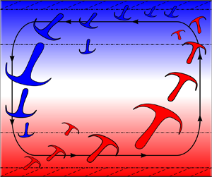
  $q_v(z) = - ({Q}/{l}) \exp (-{(h-z)}/{l})$. The injected or extracted power profile is shown in figure 1 for both cases
  $l/\delta _{T} <1$ (a) and
  $l/\delta _{T} >1$ (b). When
  $l\to 0$, this experiment becomes a standard RB experiment while, when the length
  $l$ increases, the lower and upper thermal boundary layers are heated and cooled respectively. Finally, when
  $l$ becomes greater than
  $\delta _{T}$, the bulk flow is also heated and cooled simultaneously since the lower region is heated while the upper region is cooled (figure 1b). The Rayleigh number in a modified RB experiment can be defined as in a conventional RB cell by using the temperature difference between the two plates (
 $(\rm \Delta) T = T_h - T_c$), between the lower plate and the mean bulk flow (
 $(\rm \Delta) T = 2(T_h - T_b)$) or between the mean bulk flow and the upper plate (
 $(\rm \Delta) T = 2(T_b - T_c)$). When Rayleigh numbers are high, it is assumed that the convective flow of a modified RB experiment is strong enough to impose an almost constant mean temperature over time in the bulk flow, i.e. outside the boundary layers (see figure 1), as experimentally observed in a standard RB experiment.

Figure 1. Modified RB experiment in the case of  $l / \delta _{T} <1$ (a) and in the case of
  $l / \delta _{T} >1$ (b). The heat is injected in volume near the lower plate (red zone) while the fluid is cooled in volume near the upper plate (blue area), both with a characteristic length
  $l$. The two thermal boundary layers with a width of
  $\delta _{T}$ are also displayed (hatched areas). The profiles of the volumetric (positive and negative) power source (
 $q_v$), the mean heat flux (
 $\bar {\Phi }$) and the mean temperature (
 $\bar {T}$) are also shown for each case.
A major difference between modified and standard RB experiments concerns the mean heat flux through the cell from the bottom plate to the top plate. Indeed, when a steady state is reached, the heat flux averaged over a horizontal section must be independent of the vertical coordinate ( $z$) for a standard RB experiment, whereas for a modified RB cell, this heat flux cannot be constant even in a steady state. When considering a horizontal slice of fluid, the energy given in volume must be evacuated outside the slice, which requires a gradient of the mean heat flux in the fluid (see figure 1). For
  $z=0$ and
  $z=h$, the heat flux is zero because the two horizontal plates are assumed to be perfectly insulated. Far from the plates, in the centre of the cell where
  $l \ll z \ll h-l$, the volumetric heat source
  $q_v$ is close to 0, and energy conservation leads to a heat flux equal to
  $Q \boldsymbol {e}_z$. Thus, with the exception of the blue and red regions shown in figure 1,
  $Q$ represents the heat flux through the cell and the Nusselt number can be defined as in a standard RB experiment as
 \begin{equation} Nu = \frac{Q h}{\lambda (\rm \Delta) T}, \end{equation}
where  $\lambda$ is the thermal conductivity of the fluid and
  $h$ the height of the cell. As previously mentioned, when
  $\tilde {l} \to 0$,
  $Nu$ tends towards the Nusselt number that can be obtained in the same cell but with standard RB conditions that are a constant heat flux and fixed temperatures at both plates. Hereafter, this Nusselt number will be taken as a reference and called
  $Nu_0(Ra{,Pr}) = \lim _{ \tilde {l} \rightarrow 0}Nu(Ra,{Pr}, \tilde {l})$.
Finally, it is questionable whether this type of modified RB experiment can be performed experimentally. Indeed, heating in volume can be achieved using either strong light (Lepot et al. Reference Lepot, Aumaître and Gallet2018), an electric current or even by fixing heating elements in the fluid (Kulacki & Goldstein Reference Kulacki and Goldstein1972; Goluskin Reference Goluskin2015; Goluskin & van der Poel Reference Goluskin and van der Poel2016). On the contrary, cooling in volume is more difficult to achieve experimentally. However, Lepot et al. (Reference Lepot, Aumaître and Gallet2018) and Bouillaut et al. (Reference Bouillaut, Lepot, Aumaître and Gallet2019) have shown that, in their experiments, turbulent convection develops quasi-stationary internal temperature gradients leading to a temperature difference between the lower plate and the bulk flow that is almost constant over time (see figure 1b in Lepot et al. Reference Lepot, Aumaître and Gallet2018). Therefore, the theoretical results given below will be compared in § 4 with those obtained experimentally by Lepot et al. (Reference Lepot, Aumaître and Gallet2018) and Bouillaut et al. (Reference Bouillaut, Lepot, Aumaître and Gallet2019). The theoretical model is based, on the one hand, on the known structure of the flow and temperature fields observed experimentally and numerically in a standard RB cell at high Rayleigh numbers (generally  ${>}10^6$), on the other hand, on the different theories of RB convection given in the literature.
2. Background on  $Nu$ vs $Ra$ scalings for standard RB convection


For high Rayleigh numbers, convective flow is turbulent almost everywhere in the cell except in two thin thermal boundary layers located against the lower and upper plates. This dynamic structure of the flow yields a particular field for the mean temperature. Indeed, in the bulk flow, turbulent convection produces large temporal and spatial variations for temperature fluctuations but an almost uniform mean temperature field with  $\bar {T}_b = (T_h+T_c)/2$ for symmetry reasons and assuming the Boussinesq approximation is valid (the mean temperature profile is represented in figure 1). On the contrary, the mean temperature increases or decreases by
  $(\rm \Delta) T /2 = (T_h-T_c)/2$ in each boundary layer. Therefore, the heat transfer averaged over a horizontal section is dominated by turbulent convection in the bulk flow (
 $\bar {\Phi } \approx \rho c_p \overline {w' T'}$, where
  $w'$ and
  $T'$ are the fluctuations of the vertical velocity and temperature respectively), whereas the heat transfer is driven by thermal conduction in the two thin boundary layers (
 $\bar {\Phi } \approx - \lambda \partial \bar {T} / \partial z$, where
  $\bar {T}(z)$ is the temperature averaged both on time and on a horizontal section located at the distance
  $z$ from the plate). The thickness of each thermal boundary layer (
 $\delta _{T}$) is controlled by the temperature difference
  $(\rm \Delta) T /2$ and the mean heat flux assuming that
  $\bar {\Phi }$ can be written as
  $\bar {\Phi } = \lambda (\rm \Delta) T / (2 \delta _{T})$. This last equation is valid regardless of the convection regime or the adopted theory (see Kraichnan Reference Kraichnan1962; Grossmann & Lohse Reference Grossmann and Lohse2000), leading to a ratio
  $\delta _{T} /h$ depending only on the Rayleigh number as
 \begin{equation} \frac{\delta_{T}}{h} = \frac{1}{2 Nu_0(Ra,Pr)}. \end{equation}
2.1. Classical regime by Malkus (Reference Malkus1954)
The first regime of convection, called classical, was proposed by Malkus (Reference Malkus1954) and Priestley (Reference Priestley1954). It has the merit of simplicity and predicts a scaling law  $Nu_0 \sim Ra^{1/3}$, hence with an exponent 1/3 close to the exponents observed both in the experiments and the numerical simulations in the range of
  $Ra$ between
  $10^6$ and
  $10^{12}$. This regime of convection is entirely characterized by a constant Rayleigh number for each boundary layer as
 \begin{equation} \frac{g \alpha (\rm \Delta) T \delta_{T}^3}{2 \nu \kappa} = Ra^*. \end{equation}
Using (2.1) and (2.2), we obtain for the classical regime
 \begin{equation} Nu_0 = \left (\frac{Ra}{2^4 Ra^*}\right)^{1/3}. \end{equation}
2.2. Ultimate regime by Kraichnan (Reference Kraichnan1962)
For very large Rayleigh numbers, the thermal boundary layers observed in the case of the classical regime can be destabilized and Kraichnan (Reference Kraichnan1962) and Spiegel (Reference Spiegel1971) assumed that they could become similar to the velocity boundary layers observed in the case of a fully developed mean shear flow. This ultimate regime is then characterized by a constant but Prandtl-dependent Péclet number for each thermal boundary layer
 \begin{equation} \frac{v_0^* \delta_{T}}{\kappa} = Pe^*(Pr), \end{equation}
where  $\kappa = \lambda / (\rho c_p)$ is the thermal diffusivity of the fluid. For small Prandtl numbers, the thickness of the viscous sublayer is smaller than
  $\delta _{T}$ leading to a constant Péclet number
  $Pe^* = Pe^*_{Pr \to 0}$. On the contrary, at moderate
  $Pr$ numbers,
  $Pe^*$ varies as
  $\sqrt {Pr}$ since
  $Pe^* = \sqrt {Pe^*_{Pr \to 0} Re_s Pr }$, where
  $Re_s$ is the characteristic Reynolds number for the top of the viscous sublayer (Kraichnan Reference Kraichnan1962). The new unknown parameter
  $v_0^*$ can be interpreted as a friction velocity and measures the root-mean-square value of velocity fluctuations at the edge of each boundary layer, similarly to the friction velocity defined in the case of a channel flow. Unlike the classical regime for which the characteristic Rayleigh number
  $Ra^*$ depends only on
  $(\rm \Delta) T$ and
  $\delta _{T}$,
  $Pe^*$ is linked to the convective flow in the bulk by the velocity fluctuations
  $v_0^*$. Thus, determining the Nusselt number for the ultimate regime requires additional assumptions and equations. The parameter
  $v_0^*$ is an increasing function of the large-scale mean velocity (
 $U_0$), also called as the wind turbulence. By analogy with what is well known for the channel flow, Kraichnan (Reference Kraichnan1962) assumed that
  $v_0^* \sim U_0 / \ln Re_0$, with
  $Re_0 = U_0 h / \nu$. In addition, the wind velocity is obtained by writing that the Richardson number in the bulk flow is of order 1, i.e.
  $Ri = g \alpha (\overline {w' T'}) h / U_0^3 \sim 1$. Using the definitions of
  $Re_0$,
  $Ra$ and
  $Nu_0$, this last equation yields
 \begin{equation} Re_0^3 \sim \frac{Ra Nu_0}{Pr^2}. \end{equation}
We can note that (2.5) is valid for the classical regime obtained by Malkus (Reference Malkus1954), the ultimate regime proposed by Kraichnan (Reference Kraichnan1962) and the two convection regimes (II and IV) of the Grossmann & Lohse (Reference Grossmann and Lohse2000) theory (see § 2.3). Using (2.1), (2.5) and  $v_0^* \sim U_0 / \ln Re_0$, (2.4) becomes
 \begin{equation} Re_0^2 \ln (Re_0) \sim \frac{Ra}{Pr Pe^*}. \end{equation}
Then, using (2.6), (2.5) gives the Nusselt number for the ultimate regime
 \begin{equation} Nu_0 \sim \left (\frac{Pr \, Ra}{ [ Pe^* \ln (Re_0) ]^3 }\right)^{1/2}. \end{equation}
For small  $Pr$ numbers (typically
  $Pr < Pe^*_{Pr \to 0} / Re_s$),
  $Nu_0 \sim Pr^{1/2} Ra^{1/2} / (\ln Re_0 )^{3/2}$ while for moderate
  $Pr$ numbers,
  $Nu_0 \sim Pr^{-1/4} Ra^{1/2} / [\ln (Re_0) ]^{3/2}$.
2.3. RB theory by Grossmann & Lohse (Reference Grossmann and Lohse2000)
Grossmann & Lohse (Reference Grossmann and Lohse2000) (GL) proposed a RB theory to describe with more precision the Rayleigh and Prandtl dependence of the Nusselt number. The kinetic energy and thermal dissipation rates which are defined respectively as  $\epsilon _u = ({\nu }/{2}) \sum _{i,j} (\partial _j u_i + \partial _i u_j)^2$ and
  $\epsilon _T = \kappa \sum _{i} (\partial _i T)^2$ play a central role in GL theory. In steady state and averaging over the whole RB cell the two equations of conservation of the turbulent kinetic energy (
 $\frac {1}{2}\sum _i u_i^2$) and of the square of the temperature give the following two exact relations:
 \begin{gather} \langle\epsilon_u\rangle = \frac{\nu^3}{h^4} \frac{(Nu_0 - 1) Ra}{Pr^{2}} , \end{gather}
 \begin{gather}\langle \epsilon_T \rangle = \kappa \left (\frac{(\rm \Delta) T}{h} \right )^2 Nu_0. \end{gather}
The key idea of the GL theory is to split both mean dissipation rates into two contributions each, one from the bulk (Bu) and one from the boundary layers (BLs) as
 \begin{gather} \langle\epsilon_u\rangle = \langle\epsilon_u\rangle_{Bu} + \langle\epsilon_u\rangle_{BL}, \end{gather}
 \begin{gather}\langle \epsilon_T \rangle = \langle \epsilon_T \rangle_{Bu} + \langle \epsilon_T \rangle_{BL} , \end{gather}
where
 \begin{equation} \langle\epsilon_u\rangle_{Bu} = \frac{1}{h} \int_{\delta_u}^{h-\delta_u} \overline{\epsilon_u} (z)\,\mathrm{d} z\quad \text{and}\quad \langle \epsilon_T \rangle_{Bu} = \frac{1}{h} \int_{\delta_{T}}^{h-\delta_{T}} \overline{\epsilon_T} (z)\,\mathrm{d} z \end{equation}
are, respectively, the viscous and thermal dissipation taking place in the bulk flow. Whereas the viscous and thermal dissipation taking place in the boundary layers can be written as
 \begin{equation} \langle\epsilon_u\rangle_{BL} = \frac{2}{h} \int_{0}^{\delta_u} \overline{\epsilon_u} (z)\,\mathrm{d} z\quad \text{and}\quad \langle \epsilon_T \rangle_{BL} = \frac{2}{h} \int_{0}^{\delta_{T}} \overline{\epsilon_T} (z)\,\mathrm{d} z. \end{equation}
In (2.12a,b) and (2.13a,b), the kinetic energy and thermal dissipation rates are first averaged over a horizontal cross-section giving  $\overline {\epsilon _u}$ and
  $\overline {\epsilon _T}$, respectively. The thickness of the thermal BLs (
 $\delta _T$) is given by (2.1) while a Blasius-type layer is assumed for the viscous BLs, with a thickness of
 \begin{equation} \frac{\delta_{u}}{h} = \frac{a}{\sqrt{Re_0}}. \end{equation}
Note that the prefactor  $a$ is obtained by match with a record of experimental results (Stevens et al. Reference Stevens, van der Poel, Grossmann and Lohse2013).
To obtain the Rayleigh dependence of the Nusselt and Reynolds numbers,  $\overline {\epsilon _u}$ and
  $\overline {\epsilon _T}$ need to be estimated both in the bulk flow and in the BLs
 \begin{gather} \langle{\epsilon_u}\rangle_{Bu} \sim \frac{U_0^2}{h/U_0} \left(1-\frac{\delta_u}{h} \right)\approx \frac{\nu^3}{h^4} Re_0^3, \end{gather}
 \begin{gather}\langle{\epsilon_T}\rangle_{Bu} \sim \frac{((\rm \Delta) T)^2}{h/U_0^{edge}} \left(1-\frac{\delta_T}{h} \right) \approx \kappa \left ( \frac{(\rm \Delta) T}{h} \right)^2 Re_0 Pr\,f \left( \frac{2 a Nu_0}{\sqrt{Re_0}} \right), \end{gather}
 \begin{gather}\langle{\epsilon_u}\rangle_{BL} \sim \nu \left(\frac{U_0}{\delta_u} \right )^2 \frac{\delta_u}{h} = \frac{\nu^3}{h^4} \frac{Re_0^{5/2}}{2a}, \end{gather}
 \begin{gather}\langle{\epsilon_T}\rangle_{BL} \sim \kappa \left( \frac{(\rm \Delta) T}{\delta_T}\right )^2 \frac{\delta_T}{h} = 2 \kappa \left (\frac{(\rm \Delta) T}{h}\right)^2 Nu_0. \end{gather}
In (2.16), the relevant velocity at the edge between thermal BL and the thermal bulk can be less than  $U_0$, depending on the ratio:
  $\delta _u / \delta _T = 2 a Nu_0 / \sqrt {Re_0}$. Grossmann & Lohse (Reference Grossmann and Lohse2001) introduced a function
  $0 \leq f \leq 1$ saying that the relevant velocity at the edge then becomes
  $U_0^{edge} = U_0 \,f(\delta _u / \delta _T)$, with
  $f \to 1$ when
  $\delta _u / \delta _T \to 0$ and
  $f \to 0$ for
  $\delta _u \gg \delta _T$. They gave
  $f(x) = (1 + x^n )^{-1/n}$, with
  $n\!=\!4$ as an example of function
  $f$.
$f$.
Grossmann & Lohse (Reference Grossmann and Lohse2001) have also extended those estimations of the viscous and dissipation rates for very large Prandtl numbers for which (2.14) cannot stay valid. Indeed, when  $Pr$ is high enough,
  $\delta _u$ must saturate to a maximum value
  $\delta _u(Re_c)$ lower than the height of the cell. The critical Reynolds number
  $Re_c$ was estimated from experimental data to 0.28 by Grossmann & Lohse (Reference Grossmann and Lohse2001) and 0.35 by Stevens et al. (Reference Stevens, van der Poel, Grossmann and Lohse2013). However, for the sake of simplicity, only the case of
  $Re_0 \gg Re_c$ is considered here.
From decomposition of the two global dissipation rates (2.10) and (2.11), four regimes of convection can be defined depending on whether the bulk or the BL contributions dominate the global dissipations. Besides, each of these four regimes is in principle divided into two subregimes, depending on whether the thermal BL or the kinetic BL is larger. The two  $\langle \overline {\epsilon _u}\rangle _{Bu}$ bulk-dominated regimes (referred to as II and IV) are first presented because most of the experimental and numerical results fall under one of these two regimes (see figure 8 from Stevens et al. (Reference Stevens, van der Poel, Grossmann and Lohse2013)).
2.3.1. Regimes II and IV, $\langle {\epsilon _u} \rangle \sim \langle {\epsilon _u}\rangle _{Bu}$

For regimes II and IV, the kinetic energy dissipation rate is dominated by its bulk contribution. Combining (2.8) and (2.15), and assuming  $Nu_0 \gg 1$, we obtain (2.5) again. Regime IV is obtained for high
  $Ra$ numbers for which thermal dissipation rate is dominated by its bulk contribution. Combining (2.9) and (2.16) yields
 \begin{equation} Nu_0 \sim Re_0 Pr\,f \left( \frac{2 a Nu_0}{\sqrt{Re_0}} \right)\quad \text{(Regime IV)}. \end{equation}
For lower  $Ra$ numbers, the thermal dissipation rate is dominated by its BL contribution. However, combining (2.9) and (2.18) yields a trivial equation for
  $Nu_0$. To obtain a scaling relation between
  $Nu_0$ and
  $Re_0$, Grossmann & Lohse (Reference Grossmann and Lohse2000) proposed to consider, in each thermal BL, the order of magnitude of the different terms of energy equation
 \begin{equation} u_x \partial_x T + u_z \partial_z = \kappa \partial_{zz} T. \end{equation}
Both terms on the left-hand side are of order  $U_0^{edge} (\rm \Delta) T /h$ whereas
  $\kappa \partial _{zz} T \sim \kappa (\rm \Delta) T / \delta _T^2$. Hence, using (2.1), one gets
 \begin{equation} Nu_0 \sim \sqrt{Re_0 Pr\,f \left( \frac{2 a Nu_0}{\sqrt{Re_0}} \right)} \quad \text{(Regime II)}. \end{equation}
Combining (2.5) and (2.19) or else (2.5) and (2.21), we obtain
 \begin{equation} Nu_0^{\theta_i} \sim (Nu_0 Ra Pr)^{1/3} f \left [ \frac{2a (Nu_0 Ra Pr)^{1/3} }{ (Ra /Nu_0)^{1/2} } \right ],\quad \text{with} \ \theta_{II}=2 \ \text{and} \ \theta_{IV}=1. \end{equation}
For Prandtl numbers small or large enough,  $f(x) \approx 1$ (
 $\delta _T \gg \delta _u$) or
  $f(x) \approx 1/x$ (
 $\delta _u \gg \delta _T$), and (2.22) can be simplified as follows:
 \begin{equation} {Nu_0 \sim} \begin{cases}(Ra Pr)^{1/(3\theta_i-1)},\quad \ \text{for} \ \delta_T \gg \delta_u, \\ Ra^{1/(2\theta_i+1)},\qquad \quad\text{for} \ \delta_u \gg \delta_T. \end{cases} \end{equation}
We can note that the sub-regime  $\textrm {IV}_u$ (
 $\delta _u \gg \delta _T$) gives the same scaling as predicted by Malkus (Reference Malkus1954), i.e.
  $Nu_0 \sim Pr^0 Ra^{1/3}$.
2.3.2. Regimes I and III, $\langle {\epsilon _u} \rangle \sim \langle {\epsilon _u}\rangle _{BL}$

For these two regimes, (2.5) needs to be replaced by
 \begin{equation} Re_0^{5/2} \sim \frac{Ra Nu_0}{Pr^2}. \end{equation}
Equation (2.24) is obtained by combining (2.8) and (2.17). As for regime IV, the thermal dissipation rate is dominated by its bulk contribution in regime III and (2.19) is valid. On the contrary, in regime I, we use (2.21) instead of (2.19), as for regime II. The  $Ra$- and
  $Pr$-dependent Nusselt number is then given by
 \begin{equation} Nu_0^{\theta_i} \sim (Nu_0 Ra \sqrt{Pr})^{2/5} f \left \{ \frac{2a (Nu_0 Ra \sqrt{Pr})^{2/5} } { [Ra^3 / (Nu_0^2 Pr)]^{1/5} } \right \},\quad \text{with} \ \theta_{I}=2 \ \text{and} \ \theta_{III}=1.\end{equation}
For Prandtl numbers small or large enough, (2.25) becomes
 \begin{equation}{Nu_0 \sim} \begin{cases} (Ra \sqrt{Pr})^{2/(5\theta_i-2)},\qquad \quad\text{for} \ \delta_T \gg \delta_u, \\ Ra^{3/(5\theta_i+2)} Pr^{{-}1/(5\theta_i+2)},\quad \ \text{for} \ \delta_u \gg \delta_T. \end{cases} \end{equation}
2.3.3. Grossmann & Lohse (Reference Grossmann and Lohse2001) theory for the whole parameter $(Ra,Pr)$ plane

The four previous regimes can only be observed experimentally and numerically for extreme values of  $Ra$ and
  $Pr$ numbers. For instance regime IV corresponds to very high
  $Ra$ numbers but in this case ultimate convection could appear while regime II is valid only for very small
  $Ra$ numbers for which convection is not really turbulent. Grossmann & Lohse (Reference Grossmann and Lohse2001) proposed to describe convection at any
  $Ra$ and
  $Pr$ numbers as a mixture of these four regimes. By replacing the expressions of
  $\langle {\epsilon _u}\rangle _{Bu}$ (2.15) and
  $\langle {\epsilon _u}\rangle _{BL}$ (2.17) in the balance equation for the viscous dissipation rate (2.10), they obtained this first generalised equation:
 \begin{equation} \frac{Ra Nu_0}{Pr^2} = c_1 \frac{Re_0^{5/2}}{2a} + c_2 Re_0^3. \end{equation}
Using (2.19) and (2.21), the second generalized equation can be written as
 \begin{equation} Nu_0 = c_3 \sqrt{Re_0 Pr\,f \left( \frac{2 a Nu_0}{\sqrt{Re_0}} \right)} + c_4 {Re_0 Pr\,f \left( \frac{2 a Nu_0}{\sqrt{Re_0}} \right)}. \end{equation}
Equations (2.27) and (2.28) give the dependency in  $Ra$ and
  $Pr$ of both
  $Re_0$ and
  $Nu_0$ numbers, assuming the five coefficients (
 $a$,
$a$, $c_1$–
 $c_4$) are known. Stevens et al. (Reference Stevens, van der Poel, Grossmann and Lohse2013) determined these coefficients from previous experimental measurements in the literature.
3. The $Nu$ vs $Ra$ scalings for internal source driven convection


Using the assumptions discussed below, the  $Nu$
$Nu$ $vs$
$vs$ $Ra$ scalings presented in previous section for standard RB experiments are generalized for the modified experiments described in the introduction and in figure 1. The basic assumption is to state that, for high
  $Ra$ numbers, the dynamical structure of the convective flow is the same in the standard and modified RB experiments. At a constant
  $Ra$ number, heating in volume produces the same type of thermal boundary layers as those observed in a standard RB cell. The increase in the power of the heating and cooling sources results in an increase in the bulk flow temperature, but the two types of convection experiments are so similar and the mechanisms that control the convective flow are so robust that for both classical and ultimate regimes, the values of
  $Ra^*$ and
  $Pe^*$ are identical in both types of experiments. For the GL theory, the
  $a$ parameter and the 4 dimensionless prefactors (1 by regime) are assumed to be independent of the experiment under consideration.
Secondly, in steady state, the equation of heat averaged over a horizontal section can be written as
 \begin{equation} \frac{\textrm{d} (\overline{w'T'})}{\textrm{d} z} - \lambda \frac{\textrm{d}^2 \bar{T}}{\textrm{d} z^2} = q_v(z). \end{equation}
The internal heating and cooling sources are balanced either by convective flux in the bulk flow or by a conductive flux in both boundary layers. Hereafter, only the lower boundary layer will be considered since the upper boundary layer has the same behaviour. In the boundary layer, by neglecting the convective term and using the expression of  $q_v(z)$ (see (1.1)), (3.1) can be integrated twice to obtain
 \begin{equation} T_h -\bar{T}(z) = \frac{Q h}{\lambda} \left \{ \frac{z}{h} - \frac{l}{h} [1 - \exp({-}z/l)] \right \}. \end{equation}
For  $z=\delta _{T}$ and using the definition of the Nusselt number (1.2), (3.2) yields
 \begin{equation} \frac{1}{2 Nu} = \frac{\delta_{T}}{h} - \frac{l}{h} [1 - \exp(-\delta_{T}/l)]. \end{equation}
3.1. Extension of the classical regime given by Malkus
In the classical regime by Malkus, (2.2) yields
 \begin{equation} \frac{\delta_{T}}{h} = \left ( \frac{2Ra^*}{Ra} \right )^{1/3} = \frac{1}{2 Nu_0}. \end{equation}
 \begin{equation} \frac{Nu}{Nu_0} = \frac{1}{ 1- 2 \tilde{l} Nu_0 \left[1 - \exp \left(- \dfrac{1}{2 \tilde{l} Nu_0 } \right)\right ] }. \end{equation}
In (3.4) and (3.5),  $Nu_0$ is the Nusselt number for a standard RB experiment in the classical regime but it also represents the limit of
  $Nu$ when
  $\tilde {l} = l/h \to 0$. Even if
  $Nu$ depends on both parameters
  $\tilde {l}$ and
  $Ra$, (3.5) shows that the Nusselt ratio
  $Nu / Nu_0$ is a function of a single variable that is the product of
  $\tilde {l}$ and
  $Nu_0$. This is the main result of the present theory and is tested against experimental results in § 4.
The limits of (3.5) when  $\tilde {l} \to 0$ and
  $\tilde {l} Nu_0 \gg 1$ are given in table 1. It can be noted that, when the product of
  $\tilde {l}$ and
  $Nu_0$ increases from 0 to
  $\infty$, the
  $Ra$-dependent Nusselt number (
 $Nu$) increases from a power law of one third to one of two thirds, i.e. with an exponent greater than 1/2 which characterizes the ultimate regime for a standard RB experiment (2.7).
Table 1. Limits when  $\tilde {l} Nu_0 \ll 1$ and
  $\tilde {l} Nu_0 \gg 1$ of the Nusselt number for a radiatively heated convection experiment. For the ultimate regime by Kraichnan,
  $\alpha = \ln ( Nu / Nu_0 ) / (3 \ln Re_0 )$ and
  $C_0^{{\mathcal {U}}} = {Pr } / { ( Pe^* \ln Re_0 )^3 }$. For regimes IV and III by GL, we assume that
  $\tilde {l} \ll 1$ to have
  ${\mathcal {C}} \to 0$.

3.2. Extension of Kraichnan's ultimate regime
Unlike the classical regime for which the thickness of the boundary layers depends only on  $Ra$ whatever the type of experiment considered (see (3.4)), (2.4) shows that, in the ultimate regime,
  $\delta _{T}$ depends on the velocity fluctuations in the bulk (
 $v^*$) and therefore on the thermal power injected into the bulk flow. Assuming as before that
  $v^* \sim U / \ln Re$ (Kraichnan Reference Kraichnan1962), (2.4) becomes for a modified RB experiment
 \begin{equation} \frac{\delta_{T}}{h} = \frac{Pe^*}{Pr} \frac{\ln (Re)}{ Re } = \frac{(\delta_{T})_0}{h} \frac{Re_0}{ \ln (Re_0) } \frac{\ln (Re)}{ Re }. \end{equation}
For a standard RB experiment,  $(\delta _{T})_0$ is given by (2.1) and thus (3.6) becomes
 \begin{equation} \frac{\delta_{T}}{h} = \frac{1}{2 Nu_0} \frac{Re_0}{ Re } \left [ 1 + \frac{ \ln (Re / Re_0) }{\ln (Re_0) } \right]. \end{equation}
 As assumed previously for standard RB experiments, the Richardson number in the bulk flow is taken of order 1 i.e.  $Ri = g \alpha (\overline {w' T'}) h / U^3 = g \alpha \kappa Q h / (\lambda U^3 ) \sim 1$ yielding
  $Re^3 \sim {Ra Nu / Pr^{2}}$, similarly to (2.5). Therefore, at constant Rayleigh number, the ratio of the Reynolds numbers for standard and modified RB experiments is proportional to the one-third power law of the ratio of the Nusselt numbers
 \begin{equation} \frac{Re}{Re_0} = \left ( \frac{Nu}{Nu_0} \right )^{1/3}. \end{equation}
Furthermore, (3.8) is valid both for ultimate and classical regimes of convection. Using (3.7) and (3.8), (3.3) can be written as
 \begin{equation} {\mathcal{N}}^2 = \frac{1}{ 1 + \alpha - 2\tilde{l} Nu_0 {\mathcal{N}} \left [ 1 - \exp \left ( - \dfrac{1+\alpha}{2 \tilde{l} Nu_0 {\mathcal{N}}} \right ) \right ] } , \end{equation}
where  ${\mathcal {N}} = (Nu / Nu_0 )^{1/3}$ and
  $\alpha = \ln {\mathcal {N}} / \ln Re_0$.
In the ultimate regime and similarly to the classical regime case, the ratio  $Nu / Nu_0$ is a function of the product
  $\tilde {l} \times Nu_0$. However,
  $\alpha$ also depends on the Rayleigh number through the Reynolds number
  $Re_0$. When
  $\tilde {l} \to 0$,
  $\alpha \approx 0$ since on the one hand
  ${\mathcal {N}} \to 1$ and on the other Reynolds numbers
  $Re_0$ must be large enough to reach the ultimate regime. The limit of (3.9) when
  $\tilde {l} \to 0$ is then given in table 1. For large values of
  $\tilde {l}$, (3.9) can be solved numerically for each chosen couple (
 $Ra$,
$Ra$, $\tilde {l}$) to obtain
  ${\mathcal {N}}$ and then
  $Nu$. At high
  $Nu_0$ or else at very high Rayleigh numbers,
  $Nu$ scales asymptotically as
  $Ra^2$ i.e. with an exponent 2 well above 1/2 (see table 1).
3.3. Extension of the GL theory
The balances of the turbulent kinetic energy and of the thermal variance give the following two exact relations (Shraiman & Siggia Reference Shraiman and Siggia1990; Grossmann & Lohse Reference Grossmann and Lohse2000):
 \begin{gather} \langle\epsilon_u\rangle = \frac{g \alpha}{h} \left [ \int_{0}^h \frac{\bar{\Phi}(z)}{\rho c_p} \,\mathrm{d}z - \frac{\lambda (\rm \Delta) T}{\rho c_p} \right ], \end{gather}
 \begin{gather}\langle \epsilon_T \rangle = \frac{1}{h} \int_{0}^h \bar{T}(z) \frac{q_v(z)}{\rho c_p} \,\mathrm{d}z + \frac{T_h \bar{\Phi}(0) - T_c \bar{\Phi}(h)}{\rho c_p h } . \end{gather}
Actually, for a standard RB experiment, the convective flow is driven by the thermal boundary conditions ( $(\rm \Delta) T$ or
  $\bar {\Phi }(z=0)$) whereas for the modified RB experiment presented in figure 1, the volumetric power source controls the intensity of the convective flow. Besides, for the second case, the lower and upper plates are assumed to be perfectly insulated conducting to
  $\bar {\Phi }(0) = \bar {\Phi }(h) = 0$. In steady state, energy conservation yields the following relation between the heat flux and volumetric power source:
 \begin{equation} \frac{\bar{\Phi}(z)}{Q} = \begin{cases} 1-\exp \left(-\dfrac{z}{l} \right) \quad \text{for} \ z \leq h/2 , \\ 1-\exp \left( \dfrac{h-z}{l} \right) \quad \text{for} \ h/2 \leq z \leq h.\end{cases} \end{equation}
Using (3.12) and (1.2), and assuming  $Nu \gg 1$, (3.10) becomes
 \begin{equation} \langle\epsilon_u\rangle =\frac{\nu^3}{h^4} \frac{Nu Ra}{Pr^{2}} (1 - {\mathcal{C}} ). \end{equation}
The corrective term  ${\mathcal {C}} = 2\tilde {l} [1-\exp (-{1}/{2\tilde {l}} ) ]$ only depends on
  $\tilde {l}$ and varies as
  $2\tilde {l}$ when
  $\tilde {l} \to 0$. Thus, the expression giving the dissipation rate of kinetic energy averaged over the whole cell (3.13) is very similar to that obtained for a standard RB experiment (2.8).
As for the thermal dissipation rate, its average over the cell is related to the profile of the mean temperature (3.11). As the GL theory is based on Prandtl–Blasius–Pohlhausen laminar boundary layers (Grossmann & Lohse Reference Grossmann and Lohse2000), the mean temperature can be written as
 \begin{equation} 2 \frac{\bar{T}(z) - T_b}{(\rm \Delta) T} =\begin{cases} 1 - \Theta_P \left(\dfrac{z}{\delta_T} \right) \quad \text{for} \ z \leq h/2 , \\ \Theta_P \left(\dfrac{h- z}{\delta_T} \right) - 1 \quad \text{for} \ h/2 \leq z \leq h , \end{cases} \end{equation}
with  $\Theta _P$ the Pohlhausen temperature profile which is assumed to be independent of the Prandtl number. In particular,
  $\Theta _P(0)=0$ and
  $\Theta _P(\eta )\to 1$ when
  $\eta \gg 1$. Using (3.14) and (1.1), (3.11) then becomes
 \begin{equation} \langle \epsilon_T \rangle = \kappa \left ( \frac{(\rm \Delta) T}{h} \right )^2 Nu \frac{\delta_T}{l} \int_{0}^{h/(2\delta_T)} [1-\Theta_P(\eta)] \exp \left ( -\frac{\delta_T}{l} \eta \right ) \mathrm{d} \eta . \end{equation}
Equation (3.15) shows that  $\langle \epsilon _T \rangle$ depends both on
  $\tilde {l}=l/h$ and
  $\delta _T/h$. The hypothesis adopted in § 3.1 for extending the classical regime of Malkus is again adopted here (3.4);
  $\delta _T/h$ is assumed to be only controlled by the Rayleigh number so that
  $\delta _T/h = 1/ [2 Nu_0(Ra)]$, where
  $Nu_0$ is the Nusselt number for a standard RB experiment. Equation (3.15) becomes
 \begin{equation} \langle \epsilon_T \rangle = \kappa \left ( \frac{(\rm \Delta) T}{h} \right )^2 Nu \, {\mathcal{G}}(2 Nu_0 \tilde{l}), \end{equation}
with
 \begin{equation} {\mathcal{G}}(y) = \frac{1}{y} \int_{0}^{\infty} [1-\Theta_P(\eta)] \exp \left ( -\frac{\eta}{ y} \right ) \mathrm{d} \eta . \end{equation}
Then, the central idea of the GL theory is to split the dissipation rates into two contributions (see (2.10)–(2.13a,b)). Generalization of (2.15)–(2.17) gives
 \begin{gather} \langle{\epsilon_u}\rangle_{Bu} \sim \frac{U^2}{h/U} \left(1-\frac{\delta_u}{h} \right) \approx \frac{\nu^3}{h^4} Re^3, \end{gather}
 \begin{gather}\langle{\epsilon_T}\rangle_{Bu} \sim \frac{((\rm \Delta) T)^2}{h/U^{edge}} \left(1-\frac{\delta_T}{h} \right) \approx \kappa \left ( \frac{(\rm \Delta) T}{h} \right )^2 Re Pr\,f \left( \frac{2 a Nu_0}{\sqrt{Re}} \right), \end{gather}
 \begin{gather}\langle{\epsilon_u}\rangle_{BL} \sim \nu \left(\frac{U}{\delta_u} \right )^2 \frac{\delta_u}{h} = \frac{\nu^3}{h^4} \frac{Re^{5/2}}{2a}. \end{gather}
To obtain (3.19), the relevant velocity at the edge between the thermal BL and bulk is assumed to be expressed as  $U^{edge} = U f(\delta _u / \delta _T)$, with the same function
  $f$ used for standard RB convection. Besides, we have
 \begin{equation} \frac{\delta_u}{\delta_T} = \frac{2 Nu_0 }{\sqrt{Re}}. \end{equation}
Combining (3.13) and (3.18), and using (2.5), we obtain the following first equation valid for both regimes II and IV:
 \begin{equation} \frac{Nu}{Nu_0} (1 - {\mathcal{C}} ) = \left ( \frac{Re}{Re_0} \right)^{3}\quad \text{(regimes II and IV)}. \end{equation}
Forgetting the corrective term  ${\mathcal {C}}$ which must be small since
  $\tilde {l} \ll 1$, (3.22) is the same equation as the one obtained both for extending the classical and ultimate regimes of Malkus and Kraichnan (see (3.8)). On the contrary, for regimes I and III, (3.22) needs to be replaced by
 \begin{equation} \frac{Nu}{Nu_0} (1 - {\mathcal{C}} ) = \left ( \frac{Re}{Re_0} \right)^{5/2} \quad (\text{regimes I and III}). \end{equation}
The results of this theory is first presented for regime IV because most of the experimental and numerical results fall into this regime. In addition, unlike regime II, the extension of regime IV to internally heated convection does not require the introduction of any adjustable parameters.
3.3.1. Regime IV, $\langle {\epsilon _u} \rangle \sim \langle {\epsilon _u}\rangle _{Bu}$ and $\langle {\epsilon _T} \rangle \sim \langle {\epsilon _T}\rangle _{Bu}$


For regime IV, the thermal dissipation rate is dominated by its bulk contribution. Combining (3.16) and (3.19), and using (2.19), we obtain
 \begin{equation} \frac{Nu}{Nu_0} {\mathcal{G}} (2 Nu_0 \tilde{l}) = \frac{Re}{Re_0} \frac{f ( {2 a Nu_0}/ {\sqrt{Re}}) }{f ( {2 a Nu_0}/ {\sqrt{Re_0}}) } . \end{equation}
The system of equations (3.22) and (3.24) gives the dependency of both  $Nu/Nu_0$ and
  $Re/Re_0$ as a function of the 3 control parameters:
  $Ra$,
$Ra$,  $Pr$ and
  $\tilde {l}=l/h$. For Prandtl numbers small or large enough, (3.24) can be simplified as follows:
 \begin{equation}{\frac{Nu}{Nu_0} = } \begin{cases}(1 - {\mathcal{C}} )^{-{1}/{2}} \, [{\mathcal{G}}(2 Nu_0 \tilde{l}) ]^{-{3}/{2}} ,\quad \text{for} \ \delta_T \gg \delta_u\quad (\text{regime IV}_l) \\ (1 - {\mathcal{C}} ) \, [{\mathcal{G}} (2 Nu_0 \tilde{l}) ]^{{-}2} ,\qquad\quad \text{for} \ \delta_u \gg \delta_T\quad (\text{regime IV}_u). \end{cases} \end{equation}
Besides, the limits of (3.25a) and (3.25b) when  $\tilde {l} Nu_0$ tends to 0 or
  $\infty$ can be obtained saying that
  ${\mathcal {G}}(y) \overset {y \to 0}{\approx } 1 - \Theta _P^{\prime }(0) y$ or
  ${\mathcal {G}}(y) \overset {y \to \infty }{\approx } \delta _{\Theta }^d / y$, where
  $\delta _{\Theta }^d = \int _0^{\infty } [1-\theta _P(\eta )]\, \textrm {d} \eta$. A summary of the corresponding results is given in table 1.
3.3.2. Regime II, $\langle {\epsilon _u} \rangle \sim \langle {\epsilon _u}\rangle _{Bu}$ and $\langle {\epsilon _T} \rangle \sim \langle {\epsilon _T}\rangle _{BL}$

Following the idea of Grossmann & Lohse (Reference Grossmann and Lohse2000), we consider the order of magnitude of the different terms of energy equation i.e.  $u_x \partial _x T + u_z \partial _z T = \kappa \partial _{zz} T + {q_v}/{(\rho c_p)}$. It yields
 \begin{equation} \frac{U^{edge} (\rm \Delta) T}{h} \sim \frac{\kappa (\rm \Delta) T}{\delta_T^2} + A \frac{q_v(\delta_T)}{\rho c_p}. \end{equation}
Using (1.1), (1.2), (2.1), (2.21) and  $U^{edge} = U f(\delta _u / \delta _T)$, (3.26) becomes
 \begin{equation} 1 + \tilde{A} \frac{Nu}{Nu_0} {\mathcal{H}} (2 Nu_0 \tilde{l}) = \frac{Re}{Re_0} \frac{f({2a Nu_0} / {\sqrt{Re}})}{ f({2a Nu_0} / {\sqrt{Re_0}} ) }, \end{equation}
with  ${\mathcal {H}} (y) = ({1}/{y}) \exp ( -{1}/{y} )$,
  $0\leq {\mathcal {H}} (y) \leq \exp (-1) \approx 0.37$ and
  $\tilde {A}$ a numerical constant of the order of one to be determined experimentally.
Equations (3.22) and (3.27) give the dependency of both  $Nu/Nu_0$ and
  $Re/Re_0$ as a function of
  $Ra$,
$Ra$,  $Pr$ and
  $\tilde {l}=l/h$. Contrary to the regime IV,
  $Re/Re_0$ and
  $Nu/Nu_0$ both tend towards 1 when
  $Nu_0 \tilde {l} \gg 1$ for regime II because
  ${\mathcal {H}}(y) \approx 1/y$ when
  $y\gg 1$. For the two limits
  $Nu_0 \tilde {l} \ll 1$ and
  $Nu_0 \tilde {l} \gg 1$, we obtain
 \begin{equation} \frac{Nu}{Nu_0} (1 - {\mathcal{C}} ) = 1+ \frac{\tilde{A} \, \theta_i }{ 1 - {\mathcal{C}} } {\mathcal{H}} (2 Nu_0 \tilde{l}), \end{equation}
with  $\theta _i=3$ for
  $\delta _T \gg \delta _u$ (regime
  $\textrm {II}_l$) and
  $\theta _i=2$ for
  $\delta _u \gg \delta _T$ (regime
  $\textrm {II}_u$).
For any value of  $Nu_0 \tilde {l}$, we show in appendix A that
  $Nu/Nu_0$ can be given with a very good approximation by
 \begin{equation} \frac{Nu}{Nu_0} (1 - {\mathcal{C}}) = \left [ {\mathcal{S}}_{\beta_0} \left(\frac{ \tilde{A} \, {\mathcal{H}} }{1 - {\mathcal{C}}} \right ) \right ]^3, \end{equation}
with  ${\mathcal {S}}_{\beta }(x)$ the real and positive solution of the equation:
  $1+x {\mathcal {S}}_{\beta }^3 = {\mathcal {S}}_{\beta }^{1+ \beta /2}$, and
 \begin{equation} \beta_0 = \left[\frac{2a Nu_0}{\sqrt{Re_0}} f\left( \frac{2a Nu_0}{\sqrt{Re_0}} \right) \right]^{{-}n}. \end{equation}
3.3.3. Regime I, $\langle {\epsilon _u} \rangle \sim \langle {\epsilon _u}\rangle _{BL}$ and $\langle {\epsilon _T} \rangle \sim \langle {\epsilon _T}\rangle _{BL}$


For regime I, (3.23) and (3.27) give  $Nu/Nu_0$ and
  $Re/Re_0$ as a function of
  $Ra$,
$Ra$,  $Pr$ and
  $\tilde {l}=l/h$. For the two limits
  $Nu_0 \tilde {l} \ll 1$ and
  $Nu_0 \tilde {l} \gg 1$, (3.28) is valid with
  $\theta _i=5/2$ for
  $\delta _T \gg \delta _u$ (regime
  $\textrm {I}_l$) and
  $\theta _i=5/3$ for
  $\delta _u \gg \delta _T$ (regime
  $\textrm {I}_u$).
3.3.4. Regime III, $\langle {\epsilon _u} \rangle \sim \langle {\epsilon _u}\rangle _{BL}$ and $\langle {\epsilon _T} \rangle \sim \langle {\epsilon _T}\rangle _{Bu}$

For regime III, (3.23) and (3.24) give  $Nu/Nu_0$ and
  $Re/Re_0$ as a function of
  $Ra$,
$Ra$,  $Pr$ and
  $\tilde {l}=l/h$. For Prandtl numbers large enough, we obtain
 \begin{equation} \frac{Nu}{Nu_0} = (1 - {\mathcal{C}}_{u} )^{3/2} [{\mathcal{G}} (2 Nu_0 \tilde{l}) ]^{{-}5/2}\quad \text{for} \ \delta_u \gg \delta_T\quad (\text{regime III}_u). \end{equation}
The limits of (3.31) when  $\tilde {l} \times Nu_0$ tends to 0 or
  $\infty$ are given in table 1.
3.3.5. Theory in the whole parameter $(Ra,Pr,\tilde {l})$ plane

Following the idea of Grossmann & Lohse (Reference Grossmann and Lohse2001) (see paragraph 2.3.3), at given  $Ra$,
$Ra$,  $Pr$ and
  $\tilde {l}$, radiatively driven convection can be described as a mixture of these 4 regimes. By replacing the expressions of
  $\langle {\epsilon _u}\rangle _{Bu}$ (3.18) and
  $\langle {\epsilon _u}\rangle _{BL}$ (3.20) in the balance equation for the viscous dissipation rate (3.13), the first generalized equation can be written as
 \begin{equation} \frac{Ra Nu}{Pr^2} (1 - {\mathcal{C}} ) = c_1 \frac{Re^{5/2}}{2a} + c_2 Re^3. \end{equation}
Using (3.24) and (3.29), the second generalised equation becomes
 \begin{equation} Nu = \frac{{c}_3}{ 1 - {\mathcal{C}} } \left [ {\mathcal{S}}_{\beta} \left(\frac{ \tilde{A} \, {\mathcal{H}} }{1 - {\mathcal{C}}} \right ) \right ]^3 {\sqrt{Re_0 Pr\,f \left( \frac{2 a Nu_0}{\sqrt{Re_0}} \right ) }} + \frac{{c}_4}{{\mathcal{G}}} {Re Pr\,f \left( \frac{2 a Nu_0}{\sqrt{Re}} \right)}.\end{equation}
By combining, on the one hand, (2.27) and (3.32), and, on the other hand, (2.28) and (3.33), we obtain the two equations which give  $Nu$ and
  $Re$ numbers as a function of the three parameters
  $Ra$,
$Ra$,  $Pr$ and
  $\tilde {l}$
 \begin{gather} \frac{Nu}{Nu_0} = \frac{1}{1 -{\mathcal{C}}} \frac{{c}_1 \dfrac{Re^{5/2}}{2a} + {c}_2 Re^3}{{c}_1 \dfrac{Re_0^{5/2}}{2a} + {c}_2 Re_0^3}, \end{gather}
 \begin{gather}\frac{Nu}{Nu_0} = \frac{ \dfrac{{c}_3}{ 1 - {\mathcal{C}} } \left [ {\mathcal{S}}_{\beta} \left(\dfrac{ \tilde{A} \, {\mathcal{H}} }{1 - {\mathcal{C}}} \right ) \right ]^3 {\sqrt{Re_0 Pr\,f \left( \dfrac{2 a Nu_0}{\sqrt{Re_0}} \right ) }} +\dfrac{{c}_4}{{\mathcal{G}}} {Re Pr\,f \left( \dfrac{2 a Nu_0}{\sqrt{Re}} \right)}} {c_3 \sqrt{Re_0 Pr\,f \left( \dfrac{2 a Nu_0}{\sqrt{Re_0}} \right)} + c_4 Re_0 Pr\,f \left( \dfrac{2 a Nu_0}{\sqrt{Re_0}} \right)}. \end{gather}
Figures 2( $a$) and 2(
 $b$) show the variations of the ratio
  $Nu/Nu_0$ against
  $Ra$ and
  $Pr$ for fixed values of
  $\tilde {l}$, while
  $Nu/Nu_0$ is plotted against
  $\tilde {l}$ in figure 2(
 $c$) for
  $Pr=1$ and for fixed values of
  $Ra$ between
  $10^6$ and
  $10^{14}$. As observed previously for the extensions of the Malkus and Kraichnan theories, the use of the variable
  $Nu_0 \times \tilde {l}$ allows us to gather the various curves drawn in figure 2(
 $c$) (see figure 2
 $d$). As underlined by Grossmann & Lohse (Reference Grossmann and Lohse2001) for RB convection, pure regime
  $\textrm {IV}_u$ is only reached for very high
  $Ra$ and
  $Pr$ numbers (blue upper solid line in figure 2
 $d$) while for moderate values of
  $Ra$ and
  $Pr$ numbers, radiatively heated convection is described by a mixing of the 4 regimes I–IV.

Figure 2. Results for the extension of GL theory for radiatively heated convection using (3.34) and (3.35) with  $\tilde {A}=0.3$. The coefficient
  $a$ and prefactors
  $c_1$–
 $c_4$ are given by Stevens et al. (Reference Stevens, van der Poel, Grossmann and Lohse2013). (
 $a$)
$a$)  $Nu/Nu_0$ versus
  $Ra$ for
  $Pr=0.01$ (red dotted lines) and
  $Pr=1$ (blue dashed lines), and for
  $\tilde {l} = 10^{-3}$ (lowest line),
  $\tilde {l} = 10^{-2}$ (middle line) and
  $\tilde {l} = 0.1$ (highest line). (
 $b$)
$b$)  $Nu/Nu_0$ versus
  $Pr$ for
  $Ra = 10^8$ (red dotted lines) and
  $Ra = 10^{10}$ (blue dashed lines), and for
  $\tilde {l} = 0.01$ (lowest line),
  $\tilde {l} = 0.02$ (middle line) and
  $\tilde {l} = 0.05$ (highest line). (
 $c$)
$c$)  $Nu/Nu_0$ versus
  $\tilde {l}$ for
  $Pr=1$ and for
  $Ra = 10^6$ (lowest line),
  $10^8$,
  $10^{10}$,
  $10^{12}$ and
  $10^{14}$ (highest line). (
 $d$) Same results as (
 $c$) but using
  $\tilde {l} \times Nu_0$ as
  $x$-coordinate. Also shown: regime
  $\textrm {IV}_u$ (
 $Nu/Nu_0 = {\mathcal {G}}^{-2}$) (blue solid line), regime
  $\textrm {IV}_l$ (
 $Nu/Nu_0 = {\mathcal {G}}^{-3/2}$) (blue dashed line), regime
  $\textrm {II}_u$ (red solid line) and regime
  $\textrm {II}_l$ (red dashed line).
4. Comparison with experimental results
The predictions of this theoretical approach can be tested thanks to the recent experimental investigation of Lepot et al. (Reference Lepot, Aumaître and Gallet2018) and Bouillaut et al. (Reference Bouillaut, Lepot, Aumaître and Gallet2019). The measurements cover a range of  $4 \times 10^6$ to
  $4 \times 10^9$ for
  $Ra$,
$Ra$,  $5 \times 10^{-5}$ to 0.1 for
  $\tilde {l}=l/h$ and the working fluid was water so the Prandtl number was set at a constant value close to 7. Here, the Rayleigh and Nusselt numbers are defined using
  $(\rm \Delta) T = 2(T_h - T_b)$, where
  $T_h$ and
  $T_b$ are the measured temperature of the lower plate and the bulk flow, respectively. Hence, there is a factor 2 for
  $Ra$ (and a factor 1/2 for
  $Nu$) by comparing the figures from Lepot et al. (Reference Lepot, Aumaître and Gallet2018) and Bouillaut et al. (Reference Bouillaut, Lepot, Aumaître and Gallet2019) and with those presented here. Instead of plotting
  $Nu$ as a function of
  $Ra$, the theory presented in § 3 shows that Nusselt numbers for various
  $\tilde {l}$ should better collapse around a single curve by plotting the ratio of the Nusselt numbers for modified and standard RB experiments (
 $Nu / Nu_0$) against the product of
  $\tilde {l}$ and
  $Nu_0$. As underlined by Lepot et al. (Reference Lepot, Aumaître and Gallet2018) and Bouillaut et al. (Reference Bouillaut, Lepot, Aumaître and Gallet2019), their experiments converge to RB experiments when
  $\tilde {l} \to 0$, even though the boundary conditions are very different (the horizontal plates are insulated while they are perfectly conductive for RB convection). Indeed, for
  $\tilde {l} = 5 \times 10^{-5}$, Nusselt numbers given by Bouillaut et al. (Reference Bouillaut, Lepot, Aumaître and Gallet2019) can be fitted by a simple scaling such as
  $Nu = 0.076 \times Ra^{1/3}$ with a maximum deviation of 7 %, or by the GL theory with
  $a=0.75$,
  $c_1 = 8.05$,
  $c_2 = 1.38$,
  $c_3 = 0.3$ and
  $c_4 = 0.03$. Prefactors
  $c_1$ and
  $c_2$ are the ones given by Stevens et al. (Reference Stevens, van der Poel, Grossmann and Lohse2013) while
  $c_3$ and
  $c_4$ are slightly modified to better fit to the experimental results (Stevens et al. (Reference Stevens, van der Poel, Grossmann and Lohse2013) advocated taking
  $c_3 = 0.487$ and
  $c_4 = 0.0252$). Using GL theory for defining
  $Nu_0$, the experimental results of Bouillaut et al. (Reference Bouillaut, Lepot, Aumaître and Gallet2019) are plotted in figure 3 for
  $0.0015 \leq \tilde {l} \leq 0.01$ (coloured symbols). The black dashed and blue solid lines represent, respectively, the extension of the classical scaling proposed by Malkus (Reference Malkus1954, (3.5)) and the extension of regime
  $\textrm {IV}_u$ proposed by Grossmann & Lohse (Reference Grossmann and Lohse2000, (3.25
 $b$)). First, instead of plotting
  $Nu$ against
  $Ra$ (see figure 2 in Bouillaut et al. (Reference Bouillaut, Lepot, Aumaître and Gallet2019)), plotting compensated Nusselt numbers
  $Nu/Nu_0$ as a function of
  $\tilde {l} Nu_0 \sim \tilde {l} Ra^{1/3}$ allows the collapse of the experimental data onto a single curve. Secondly, this curve is given by (3.5) or (3.25b) with a fairly good accuracy and without the use of any adjustable parameter. The system of equations (3.34) and (3.35) that results from a mixture of regimes I to IV and is represented by grey symbols in figure 3 gives slightly lower values for the ratio
  $Nu / Nu_0$ than the pure regime IV (blue solid line). The new parameter
  $\tilde {A}$ has little impact on the curve for these data set and is fixed to 0.35 in figure 3. In view of: (i) the experimental uncertainties, (ii) the product
  $\tilde {l} \times Nu_0$ being always less than 5 and (iii)
  $Pr$ number being fixed to 7 for the experimental results, it is difficult to discriminate between the different extensions of the theoretical models presented in § 3 describing convection in classical regimes.

Figure 3. Compensated Nusselt numbers for a radiatively heated convection experiment as a function of  $\tilde {l} Nu_0$. Coloured symbols: experiments from Bouillaut et al. (Reference Bouillaut, Lepot, Aumaître and Gallet2019) with
  $\tilde {l}=0.0015$ (
 $\star$),
  $\tilde {l}=0.003$ (
 $+$),
$+$),  $\tilde {l}=0.006$ (
 $\Diamond$),
  $\tilde {l}=0.0012$ (
 $*$),
$*$),  $\tilde {l}=0.0024$ (
 $\square$),
  $\tilde {l}=0.048$ (
 $\rhd$),
  $\tilde {l}=0.05$ (
 $\circ$),
  $\tilde {l}=0.096$ (
 $\nabla$). Black dashed line: extension of the classical regime by Malkus (Reference Malkus1954, (3.5)), no adjustable parameter. Blue solid line: extension of the regime
  $\textrm {IV}_u$ by Grossmann & Lohse (Reference Grossmann and Lohse2000, (3.25
 $b$)) with
  ${\mathcal {C}}=0$, no adjustable parameter. Grey symbols: (3.34) and (3.35) with
  $\tilde {A} =0.35$. Upper red lines: extension of the ultimate regime by Kraichnan (Reference Kraichnan1962, (3.9)) with
  $Re_0=1000$ (red dotted line) and
  $Re_0=10^{10}$ (red dashed line).
On the contrary, it is well known that convection in the so-called ultimate regime behaves very differently since  $Nu_0$ scales asymptotically as
  $Ra^{1/2}$, thus with an exponent 1/2 much higher than 1/3. The theoretical work presented in § 3 shows that, for radiatively heated convection, there is also a clear difference for the ratio
  $Nu/Nu_0$ between classical regimes and the ultimate regime. In figure 3, the two upper red lines represent the ultimate regime (3.9) for two fixed Reynolds numbers (dotted line:
  $Re_0=1000$, dashed line:
  $Re_0=10^{10}$). They are clearly above all other curves and symbols describing the theoretical and experimental results for classical regimes. Indeed,
  $Ra$ numbers achieved by the experiments of Bouillaut et al. (Reference Bouillaut, Lepot, Aumaître and Gallet2019) are not sufficient to trigger the ultimate regime (a detailed discussion is given in appendix B).
5. Conclusions
The well-known theories of RB convection have been extended here to radiatively heated convection. The evolution of the Nusselt number as a function of  $Ra$,
$Ra$,  $Pr$ and
  $l/h$ (where
  $l$ is the heating length near the lower plate and
  $h$ the height of the cell) is predicted whatever the convection regime considered. In the classical regime and using the simple theory of Malkus (Reference Malkus1954), equation (3.5) gives
  $Nu / Nu_0$ as a function of
  $Ra$ and
  $l/h$ without an adjustable parameter, while, considering the more recent Grossmann & Lohse (Reference Grossmann and Lohse2000) theory, the two equations (3.34) and (3.35) give the dependency of both
  $Nu/Nu_0$ and
  $Re/Re_0$ as a function of the 3 control parameters
  $Ra$,
$Ra$,  $Pr$ and
  $l/h$. It can be noted that only the extension of regimes I and II of the GL theory, observable only at low
  $Ra$ numbers, needs an adjustable parameter. A good agreement is observed between the experimental results obtained by Bouillaut et al. (Reference Bouillaut, Lepot, Aumaître and Gallet2019) and the theoretical results for the classical regime. For the ultimate regime, equation (3.9) gives the Nusselt number as a function of
  $Ra$ and
  $l/h$ without an adjustable parameter, but, in this case, no experimental or numerical results exist to test this prediction. Finally, this work predicts that the Nusselt number behaves asymptotically as
  $Ra^{2/3}$ or
  $Ra$ for the classical regime (see table 1) while it scales as
  $Ra^{2}$ in the ultimate regime, and this prediction is of major interest for geophysical and astrophysical flows where convection is driven by internal heat sources.
Acknowledgements
B. Castaing is gratefully thanked for his suggestions and the review of the article.
Declaration of interests
The author reports no conflict of interest.
Appendix A. Extension of regime II of the GL theory
For regime II, (3.22) and (3.27) give the dependency of both  $Nu/Nu_0$ and
  $Re/Re_0$ as a function of
  $Ra$,
$Ra$,  $Pr$ and
  $\tilde {l}=l/h$. Using (3.22), (3.27) becomes
 \begin{equation} 1 + \frac{\tilde{A} \, {\mathcal{H}}}{1 - {\mathcal{C}}} \left ( \frac{Re}{Re_0} \right)^{3} = \frac{Re}{Re_0} \frac{f \left( \dfrac{2 a Nu_0}{\sqrt{Re}} \right )}{ f \left( \dfrac{2 a Nu_0}{\sqrt{Re_0}} \right ) }. \end{equation}
A.1. Regime $\textrm {II}_u$ (high $Pr$ numbers or $\delta _u \gg \delta _T)$


Equation (A 1) becomes
 \begin{equation} 1 + \frac{\tilde{A} \, {\mathcal{H}}}{1 - {\mathcal{C}}} \left ( \frac{Re}{Re_0} \right)^{3} = \left (\frac{Re}{Re_0}\right)^{3/2}. \end{equation}
To get a positive value for  $Re$, we must have:
  $\tilde {A} {\mathcal {H}} \leq (1 - {\mathcal {C}})/4 \leq 1/4$. As
  ${\mathcal {H}}\leq \exp (-1)$, the parameter
  $\tilde {A}$ needs to be lower than
  $\exp (1)/4 \approx 0.68$. Resolution of (A 2) gives
 \begin{equation} \frac{Re}{Re_0} = {\mathcal{S}}_u \left(\frac{ \tilde{A} \, {\mathcal{H}} }{1 - {\mathcal{C}}} \right ), \end{equation}
with  ${\mathcal {S}}_u(x) = ({(1-\sqrt {1- 4x})}/{2x} )^{2/3}$;
  ${\mathcal {S}}_u(x)$ is an increasing function of
  $x$ with
  ${\mathcal {S}}_u(0) = 1$ and
  ${\mathcal {S}}_u(1/4) = 2^{2/3} \approx 1.59$, yielding
  $1 \leq Re/Re_0 \leq 1.59$.
A.2. Regime $\textrm {II}_l$ (low $Pr$ numbers or $\delta _T \gg \delta _u$)


Equation (A 1) becomes
 \begin{equation} 1 + \frac{\tilde{A} \, {\mathcal{H}}}{1 - {\mathcal{C}}} \left ( \frac{Re}{Re_0} \right)^{3} = \frac{Re}{Re_0}. \end{equation}
To get a positive value for  $Re$, we must have:
  $\tilde {A} {\mathcal {H}} \leq 4(1 - {\mathcal {C}})/27 \leq 4/27$. As
  ${\mathcal {H}}\leq \exp (-1)$, the parameter
  $\tilde {A}$ needs to be lower than
  $4 \exp (1)/27 \approx 0.40$. Resolution of (A 4) gives
 \begin{equation} \frac{Re}{Re_0} = {\mathcal{S}}_l \left(\frac{ \tilde{A} \, {\mathcal{H}} }{1 - {\mathcal{C}}} \right ), \end{equation}
with
 \begin{equation} {\mathcal{S}}_l(x) = \frac{2}{\sqrt{3x}} \cos \left[ \frac{1}{3} \arccos \left( \frac{3 \sqrt{3x}}{2} \right) + \frac{\rm \pi}{3} \right]. \end{equation}
Here,  ${\mathcal {S}}_l(x)$ is an increasing function of
  $x$ with
  ${\mathcal {S}}_l(0) = 1$ and
  ${\mathcal {S}}_l(4/27) = 3/2$ yielding
  $1 \leq Re/Re_0 \leq 3/2$.
A.3. Approximation of (A 1) for any $Pr$ numbers

For the two limits  $Pr\gg 1$ and
  $Pr \ll 1$, we have shown that
  ${1 \leq Re/Re_0 \leq 3/2}$. The following approximation can then be adopted:
  $f(x_0) \approx f(x) ( {x}/{x_0} )^{-\beta _0}$, with
  $\beta _0 = - ({\textrm {d} \ln f }/{\textrm {d} \ln x} )_{x=x_0} = [x_0 f(x_0)]^{-n}$ (
 $n=4$). When
  $x_0 \gg 1$,
  $\beta _0 \to 3/2$ while
  $\beta _0 \to 0$ when
  $x_0 \to 0$. Equation (A 1) can therefore be approximated by
 \begin{equation} 1 + \frac{\tilde{A} \, {\mathcal{H}}}{1 - {\mathcal{C}}} \left ( \frac{Re}{Re_0} \right)^{3} = \left (\frac{Re}{Re_0} \right)^{1+ \beta_0/2}. \end{equation}
By calling  ${\mathcal {S}}_{\beta }(x)$ the real and positive solution of the equation:
  $1+x {\mathcal {S}}_{\beta }^3 = {\mathcal {S}}_{\beta }^{1+ \beta /2}$, we obtain
 \begin{equation} \frac{Re}{Re_0} = {\mathcal{S}}_{\beta_0} \left(\frac{ \tilde{A} \, {\mathcal{H}} }{1 - {\mathcal{C}}} \right ), \end{equation}
with
 \begin{equation} \beta_0 = \left[ \frac{2a Nu_0}{\sqrt{Re_0}} f\left( \frac{2a Nu_0}{\sqrt{Re_0}} \right)\right]^{{-}n}. \end{equation}
Using (A 8), (3.22) gives the variations of  $Nu/Nu_0$ as a function of
  $Ra$,
$Ra$,  $Pr$ and
  $\tilde {l}$ in regime II (3.29). These variations are plotted in figure 4(
 $a$) with
  $\tilde {A} = 4 \exp (1)/27 \approx 0.40$ and in figure 4(
 $b$) with
  $\tilde {A} = 0.35$. For each case, we can note that (3.29) (represented by black solid lines) is a good approximation of the solution of the system of (3.22) and (3.27) (grey symbols). That is why (3.29) is used in § 3.3.5 to extent GL theory to radiatively heated convection in the whole parameter
  $(Ra,Pr,\tilde {l})$ plane.

Figure 4. Value of  $Nu/Nu_0$ versus
  $\tilde {l} Nu_0$ in regime II of the extended GL theory for radiatively heated convection. Grey symbols: solution of (3.22) and (3.27) with
  ${\mathcal {C}} = 0$,
  $\tilde {A} = 4 \exp (1)/27 \approx 0.40$ (
 $a$) and
  $\tilde {A} = 0.35$ (
 $b$). Black solid lines: (3.29). From top to bottom, the parameter
  $2a Nu_0 / \sqrt {Re_0}$ is taken to be equal to 0.5, 1 and 1.5. The lower solid red line represents regime
  $\textrm {II}_u$ while the upper dashed red line shows regime
  $\textrm {II}_l$.
Appendix B. Discussion of the model and scaling proposed by Bouillaut et al. (Reference Bouillaut, Lepot, Aumaître and Gallet2019)
Bouillaut et al. (Reference Bouillaut, Lepot, Aumaître and Gallet2019) proposed a simple model to describe radiatively driven convection leading to the scaling relation  $Nu \sim \tilde {l} (Ra Pr) ^{1/2}$. The theory presented in § 3 shows that the scaling
  $Nu \sim Ra^{1/2}$ can only be observed for a limited range of
  $Ra$ for each
  $\tilde {l}$ considered. Indeed, using for example (3.5),
  $Nu$ scales as
  $Ra^{1/3}$ when
  $\tilde {l} \to 0$ while it scales as
  $Ra^{2/3}$ when
  $\tilde {l} \times Ra^{1/3}$ is quite high. Thus, for a limited range of
  $Ra$,
$Ra$,  $Nu$ can be fitted by
  $Ra^{1/2}$ but this scaling cannot be observed asymptotically. Bouillaut et al. (Reference Bouillaut, Lepot, Aumaître and Gallet2019) have also proposed representing the experimental data considering the product of
  $Nu$ and
  $\tilde {l}^2$ as a function of the product of
  $Ra$ and
  $\tilde {l}^6$ (see figure 5
 $a$). The theory presented here shows that, in this representation, the experimental data can only collapse on a single curve if both the range of
  $Ra$ is relatively small and this range is the same for all the
  $\tilde {l}$ investigated. On the contrary, (3.5) predicts that
  $Nu \, \tilde {l}$ depends only on
  $Nu_0 \, \tilde {l}$ or only on
  $Ra \, \tilde {l}^3$ assuming
  $Nu_0 \sim Ra^{1/3}$ (2.3). Besides, in this representation (figure 5
 $b$), the curve is given by (3.5) and without any adjustable parameter.

Figure 5. Comparison of the scaling proposed by Bouillaut et al. (Reference Bouillaut, Lepot, Aumaître and Gallet2019) ( $a$) and the model described in § 3 (
 $b$). Symbols as in figure 3. Dotted lines: (3.5), without an adjustable parameter.


