


1 Introduction
The study of the shape and stability of a free surface of fluid at rest is an important field of fluid mechanics. The description and classification of the shapes of soap films supported by the wire frames (see figure 1a–d) is called the Plateau problem, named after the Belgian physicist Joseph Plateau who discovered many surprising phenomena associated with this seemingly simple system (Plateau Reference Plateau1863, Reference Plateau1873). The soap film takes on a shape which minimizes its surface area, hence the Plateau problem is equivalent to the problem of finding minimal surfaces. Mathematically, one has to find a surface with zero mean curvature with the boundary conditions stating that the surface must touch the given frame (Thi & Fomenko Reference Thi and Fomenko1991; Courant Reference Courant2005; Nitsche Reference Nitsche2011).
The classical Plateau problem has a distinguished history and finds numerous applications. In particular, soap films supported by solid frames of different shapes can be used to generate the fundamental periodic cell of the translation symmetry group of triply periodic minimal surfaces (TPMS) (Courant Reference Courant2005; Nitsche Reference Nitsche2011). An example of such a periodic cell is shown in figure 1(e,f), where the surface is supported by the triangular frames. Filling the whole space with the obtained hexagonal cells, one obtains the so-called Schwarz’s H TPMS (Nitsche Reference Nitsche2011).

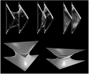
Figure 1. (a) The catenoid is a classical minimal surface formed by a soap film between two coaxial circular wire rings of 25 mm diameter. (b) Soap film supported by two triangular equilateral wire frames with the 25 mm long side. (c) Soap films can form complex periodic structures such as those shown here using the triangular frames from (b). (d) Minimal surface on the L-shaped frame ( $20\times 20\times 50~\text{mm}$) analytically described by Chaplygin. (e) An example illustrating the construction of a TPMS taking (b) as a generator and rotating the obtained minimal surface about the sides of the triangle by
  $180^{\circ }$. First, from a single generating cell one obtains a double-cell structure. Then, one forms a hexagonal cell using the double-cell constructs; see the movie in the supplementary material available online at https://doi.org/10.1017/jfm.2020.391. This hexagonal cell is used to generate a TPMS. (f) The side and top views of the obtained periodic cell of TPMS.
Minimal surfaces, having their principal curvatures equal in magnitude and opposite in sign at all points on the surface, have been found in many natural systems and inspired generations of engineers to use them in practical applications (Hildebrandt & Tromba Reference Hildebrandt and Tromba1986; Andersson et al. Reference Andersson, Hyde, Larsson and Lidin1988; Klinowski, Mackay & Terrones Reference Klinowski, Mackay and Terrones1996; Lord, Mackay & Ranganathan Reference Lord, Mackay and Ranganathan2006; Nitsche Reference Nitsche2011; Han & Che Reference Han and Che2018). New experiments on moving liquid films have ignited the interest of the fluid mechanics community in periodic minimal surfaces (Chen & Steen Reference Chen and Steen1997; Buckingham & Bush Reference Buckingham and Bush2001; Clanet Reference Clanet2001; Dressaire et al. Reference Dressaire, Courbin, Delancy, Roper and Stone2013).
The main progress in the analytical description and classification of TPMS has been done using the Weierstrass representation of minimal surfaces given in the parametric form as the real part of the complex-valued integrals
 $$\begin{eqnarray}\displaystyle & \displaystyle x(\unicode[STIX]{x1D714})=\text{Re}\int _{\unicode[STIX]{x1D714}_{0}}^{\unicode[STIX]{x1D714}}(1-\unicode[STIX]{x1D714}^{2})R(\unicode[STIX]{x1D714})\,\text{d}\unicode[STIX]{x1D714},\quad y(\unicode[STIX]{x1D714})=\text{Re}\int _{\unicode[STIX]{x1D714}_{0}}^{\unicode[STIX]{x1D714}}i(1+\unicode[STIX]{x1D714}^{2})R(\unicode[STIX]{x1D714})\,\text{d}\unicode[STIX]{x1D714}, & \displaystyle \nonumber\\ \displaystyle & \displaystyle z(\unicode[STIX]{x1D714})=\text{Re}\int _{\unicode[STIX]{x1D714}_{0}}^{\unicode[STIX]{x1D714}}2\unicode[STIX]{x1D714}R(\unicode[STIX]{x1D714})\,\text{d}\unicode[STIX]{x1D714}, & \displaystyle \nonumber\end{eqnarray}$$
 where  $(x,y,z)$ are the Cartesian coordinates of a point on the minimal surface and
  $R(\unicode[STIX]{x1D714})$ is the Weierstrass function of a complex variable
  $\unicode[STIX]{x1D714}$ (for an introduction to this method see Nitsche Reference Nitsche2011). The Weierstrass formulas provide a general representation of surfaces using an a priori unknown function
  $R(\unicode[STIX]{x1D714})$, the generation function; thus, the minimal surface description is reduced to an analysis of the surface shapes represented by the Weierstrass formulas by guessing different generation functions. This is an inverse boundary value problem which does not give a straightforward recipe for calculating the minimal surface of interest; fortunately, in a series of papers (Fogden & Hyde Reference Fogden and Hyde1992a,Reference Fogden and Hydeb; Fogden Reference Fogden1993), Hyde and Fogden explained how to identify and numerically calculate a broad class of TPMS generated by polygonal frames. It remains questionable whether these surfaces are stable and could be realized in experiments. Karcher discovered another way to generate a new class of TPMS taking the available explicit representations of known TPMS and generating new ones by combining them in a special way (Karcher Reference Karcher1989; Karcher & Polthier Reference Karcher and Polthier1996). Existing methods based on the Weierstrass parametrization and related approaches generate surfaces which may have self-intersections. Hence, while this methodology is very attractive from the geometrical perspective, it requires a significant effort to eliminate self-intersecting minimal surfaces and specify the physical properties of the generated surfaces and their stability.
Chaplygin, in the last chapter of his fundamental work (Chaplygin Reference Chaplygin1904, Reference Chaplygin1944), noticed that the two-dimensional flow equations for a fictitious gas also describe some minimal surfaces. This analogy appears quite useful for investigation of geometrical properties of minimal surfaces (Bers Reference Bers1951a,Reference Bersb, Reference Bers2016; Dierkes, Hildebrandt & Tromba Reference Dierkes, Hildebrandt and Tromba2010; Nitsche Reference Nitsche2011). Without any derivation and figures, Chaplygin gave analytical formulas describing a minimal surface supported by the L-shaped frame shown in figure 1(d). This example has been forgotten and, to the best of our knowledge, never been mentioned in the literature on minimal surfaces. We recently revisited Chaplygin’s method, applying it to study stability of soap films supported by circular rings (Alimov & Kornev Reference Alimov and Kornev2019).
In the present paper, we generalize Chaplygin’s method to study minimal surfaces generated by the polygonal frames. As an illustration of the proposed methodology, we study theoretically and experimentally the shape and stability of soap films supported by equilateral triangular frames (figure 1b). This minimal surface has been identified earlier as a model system for demonstration of the robustness of the parametrization algorithms for the Weierstrass method (Lidin Reference Lidin1988; Cvijovic & Klinowski Reference Cvijovic and Klinowski1992a,Reference Cvijovic and Klinowskib), but the stability analysis of these surfaces has never been performed. We, therefore, fill this gap and present the critical separation distance when the minimal surface will break up. These results are given not only for triangular frames, but for any equilateral supporting polygons. First, in §§ 2–3, we formulate the Plateau problem closely following Chaplygin’s method and using the developments of his method in the theory of flow of non-Newtonian fluids through porous media, as partially discussed in Goldstein & Entov (Reference Goldstein and Entov1994). The calculations necessary for the hodograph formulation of the Plateau problem are given in §§ 2–3 and in the supplementary material. They are missing in the Chaplygin (Reference Chaplygin1904, Reference Chaplygin1944) and Goldstein & Entov (Reference Goldstein and Entov1994) books. The theory developed in §§ 4–7 is new. In § 8, we experimentally study the shapes of the soap films formed on triangular frames and compare the theoretical shapes to show an excellent fit confirming the theory.
Presenting an explicit solution for the surfaces supported by equilateral  $n$-gons, we enrich the class of TPMS crystals for which the closed-form analytical representation is available (Cvijovic & Klinowski Reference Cvijovic and Klinowski1992a,Reference Cvijovic and Klinowskib; Karcher & Polthier Reference Karcher and Polthier1996; Klinowski et al. Reference Klinowski, Mackay and Terrones1996; Nitsche Reference Nitsche2011) and open up a new opportunity for the development of analytical classification of minimal surfaces using a rich arsenal of methods of ideal gas fluid mechanics.
2 The Plateau problem as a free boundary value problem for the mean curvature equation
The minimal surface,  $\unicode[STIX]{x1D6F4}$, consists of two identical frames of equilateral
  $n$-polygons
  $(n\geqslant 3)$. The frames are parallel to each other and their centroids are sitting on the same axis; this axis is chosen as the
  $z$-axis of Cartesian coordinates. We will use a triangular frame as an illustrative example of the geometrical constructions (figure 2). This example bears all the necessary elements of the general
  $n$-sided polygons, yet it demonstrates the most important features distinguishing these minimal surfaces from a catenoid (Chen & Steen Reference Chen and Steen1997; Arfken, Weber & Harris Reference Arfken, Weber and Harris2012; Alimov & Kornev Reference Alimov and Kornev2019), a minimal surface supported by two circular frames. The centre of Cartesian coordinates, point
  $O$ in figure 2, corresponds to the centroid of the lower frame.

Figure 2. (a) Schematic of a minimal surface supported by two parallel frames  $A_{1}A_{2}A_{3}$ and
  $A_{1}^{\prime }A_{2}^{\prime }A_{3}^{\prime }$. The surface
  $\unicode[STIX]{x1D6F4}$ is mirror symmetric with respect to the midplane passing through point
  $O^{\prime }$. The dashed curve shows the contour of a neck
  $\unicode[STIX]{x1D6E4}$ of this minimal surface, the plane
  $O^{\prime }CD$ is parallel to the planes
  $A_{1}A_{2}A_{3}$ and
  $A_{1}^{\prime }A_{2}^{\prime }A_{3}^{\prime }$. The dashed lines
  $DA_{1}$ and
  $CB$ mark the
  $\unicode[STIX]{x1D6F4}$ fundamental patch of symmetry: the entire surface is obtained by the mirror-symmetric reflections of surface
  $A_{1}BCDA_{1}$ with respect to vertical planes, formed by the medians of triangular frames as well as with respect to the horizontal plane
  $O^{\prime }CD$. The vector
  $\boldsymbol{N}$ is an outward unit normal vector to the surface
  $\unicode[STIX]{x1D6F4}$ at any point on the surface and the vector
  $\boldsymbol{J}$ is the
  $xy$-projection of vector
  $\boldsymbol{N}$. (b) Schematic of a minimal surface supported by two parallel frames
  $A_{1}A_{2}A_{3}$ and
  $A_{1}^{\prime }A_{2}^{\prime }A_{3}^{\prime }$; the surface is partitioned by a lamella
  $\unicode[STIX]{x1D6F4}_{3}$ – a flat film supported by the Plateau ring
  $\unicode[STIX]{x1D6E4}$. This lamella belongs to the plane
  $O^{\prime }CD$. Two surfaces
  $\unicode[STIX]{x1D6F4}_{1}$ and
  $\unicode[STIX]{x1D6F4}_{2}$ are mirror symmetric with respect to plane
  $O^{\prime }CD$ and they meet at ring
  $\unicode[STIX]{x1D6E4}$ forming
  $2\unicode[STIX]{x03C0}/3$ angle. (c) Projection of
  $1/12$ of the surface
  $\unicode[STIX]{x1D6F4}$,
  $A_{1}BCDA_{1}$, on the
  $xy$-plane. The shaded area
  $A_{1}BCDA_{1}$ can be considered as the shadow of the minimal surface when the light is shining parallel to the
  $z$-axis;
  $|A_{1}B|=|A_{3}B|$. For any equilateral polygons, the angle
  $\unicode[STIX]{x1D6FD}_{n}$ in the right triangle
  $OA_{1}B$ at the centroid
  $O$, is
  $\unicode[STIX]{x1D6FD}_{n}=\unicode[STIX]{x03C0}/n$,
  $n\geqslant 3$. The vector
  $\boldsymbol{J}$, the projection of normal vector
  $\boldsymbol{N}$ on the
  $xy$-plane is specified by the angle
  $\unicode[STIX]{x1D703}$ formed by
  $\boldsymbol{J}$ and the
  $x$-axis. The direction of vector
  $\boldsymbol{J}$ is completely specified at the sides of polygon
  $A_{1}BCDA_{1}$, but its direction is unknown at the neck contour
  $\unicode[STIX]{x1D6E4}$, except it is known that
  $\boldsymbol{J}$ is perpendicular to
  $\unicode[STIX]{x1D6E4}$.
For equilateral polygons, the minimal surface  $\unicode[STIX]{x1D6F4}$ is mirror symmetric with respect to any plane passing through the angle bisectors perpendicularly to the frames; in figure 2, for example, the plane
  $A_{2}OO^{\prime }$ is the plane of symmetry.
Let  $A_{1},\ldots ,A_{n}$ be the vertices of the lower polygon, and let the
  $x$-axis pass through
  $A_{1}$. Introduce point
  $B$ that splits the side
  $A_{1}A_{n}$ into halves,
  $|A_{1}B|=|A_{n}B|$. The length will be measured in terms of the radius of a circle that encloses the polygon,
  $|OA_{1}|=r$. Thus, introducing dimensionless variables,
  $x=X/r$,
  $y=Y/r$,
  $z=Z/r$, we will have in dimensionless coordinates
 $$\begin{eqnarray}|OA_{1}|=1.\end{eqnarray}$$
 As shown in our experiments, for certain conditions discussed below, the continuous surface  $\unicode[STIX]{x1D6F4}$ can spontaneously form a lamella splitting this surface in two mirror-symmetric parts, as shown in figure 2(b). The smooth parts
  $\unicode[STIX]{x1D6F4}_{1}$ and
  $\unicode[STIX]{x1D6F4}_{2}$ meet at the Plateau angle (Plateau Reference Plateau1863, Reference Plateau1873) of
  $2\unicode[STIX]{x03C0}/3$. We confirm this observation of Plateau below. Thus, there are two possibilities for shaping of the minimal surfaces supported by equilateral polygons, both of which will be analysed in detail using the proposed Chaplygin hodograph formulation.
For equilateral polygons, the angle  $\unicode[STIX]{x1D6FD}_{n}$ in the right triangle
  $OA_{1}B$ at the centroid
  $O$, is (figure 2c)
 $$\begin{eqnarray}\unicode[STIX]{x1D6FD}_{n}=\unicode[STIX]{x03C0}/n,\quad n\geqslant 3.\end{eqnarray}$$
 We will work only with a fundamental symmetry patch (like  $A_{1}BCDA_{1}$ in figure 2) where the height of the surface with respect to the lower frame is represented as
 $$\begin{eqnarray}z=h(x,y).\end{eqnarray}$$
 This function is defined in domain  $\unicode[STIX]{x1D6FA}$ as illustrated in figure 2(c). The normal vector
  $\boldsymbol{N}=(1+|\unicode[STIX]{x1D735}h|^{2})^{-1/2}(-\unicode[STIX]{x2202}h/\unicode[STIX]{x2202}x,-\unicode[STIX]{x2202}h/\unicode[STIX]{x2202}y,1)$ to the surfaces
  $\unicode[STIX]{x1D6F4}_{1}$ and the projection
  $\boldsymbol{J}=-(1+|\unicode[STIX]{x1D735}h|^{2})^{-1/2}\unicode[STIX]{x1D735}h$ of the normal vector
  $\boldsymbol{N}$ on the
  $xy$-plane are defined through the two-dimensional gradient operator
  $\unicode[STIX]{x1D735}=(\unicode[STIX]{x2202}/\unicode[STIX]{x2202}x,\unicode[STIX]{x2202}/\unicode[STIX]{x2202}y)$. The mean curvature (2.3) is defined as
  $\unicode[STIX]{x1D705}=\unicode[STIX]{x1D735}\boldsymbol{\cdot }\boldsymbol{J}=-\unicode[STIX]{x1D735}\boldsymbol{\cdot }[(1+|\unicode[STIX]{x1D735}h|^{2})^{-1/2}\unicode[STIX]{x1D735}h]$. To find function
  $z=h(x,y)$, we need to solve the nonlinear mean curvature equation
  $\unicode[STIX]{x1D705}=0$:
 $$\begin{eqnarray}\unicode[STIX]{x1D6FA}:\quad \unicode[STIX]{x1D735}\boldsymbol{\cdot }[(1+|\unicode[STIX]{x1D735}h|^{2})^{-1/2}\unicode[STIX]{x1D735}h]=0.\end{eqnarray}$$
 The necessary conditions for smooth mirror-symmetric continuation of function  $h(x,y)$ through the boundary
  $A_{1}D$ and, consequently, through
  $BC$ require the following boundary conditions
 $$\begin{eqnarray}\displaystyle & \displaystyle A_{1}D:\quad \unicode[STIX]{x2202}h/\unicode[STIX]{x2202}y=0, & \displaystyle\end{eqnarray}$$
 $$\begin{eqnarray}\displaystyle & \displaystyle BC:\quad \unicode[STIX]{x2202}h/\unicode[STIX]{x2202}n_{BC}=0. & \displaystyle\end{eqnarray}$$
The height at the lower frame is known,
 $$\begin{eqnarray}A_{1}B:\quad h=0,\end{eqnarray}$$
 and the height of the neck is  $H/2$, as it is located between two frames separated by the distance
  $H$. The shape of curve
  $\unicode[STIX]{x1D6E4}=CD$ is unknown in advance and has to be found as a part of the solution, i.e. the boundary
  $\unicode[STIX]{x1D6E4}$ is a free boundary. Thus, we have two boundary conditions at
  $\unicode[STIX]{x1D6E4}$. We need to employ one more condition stating that the surface approaches the neck contour vertically
 $$\begin{eqnarray}\unicode[STIX]{x1D6E4}:\quad h=\frac{H}{2},\quad |\unicode[STIX]{x1D735}h|\rightarrow \infty .\end{eqnarray}$$
 The second condition (2.8) has to be modified for the case of a surface partitioned by the lamella (figure 2b). The Plateau law (Plateau Reference Plateau1863, Reference Plateau1873) requires the normal vectors  $\boldsymbol{N}$ to the surfaces
  $\unicode[STIX]{x1D6F4}_{1}$ and
  $\unicode[STIX]{x1D6F4}_{2}$ at the common contour
  $\unicode[STIX]{x1D6E4}$ to form a
  $2\unicode[STIX]{x03C0}/3$ angle. The projection of the normal vector
  $\boldsymbol{N}$ on the
  $xy$-plane defines vector
  $\boldsymbol{J}$ (figure 2a). Therefore, projecting vector
  $\boldsymbol{N}$ on the
  $xy$-plane, we have
  $J=|\boldsymbol{J}|=|\boldsymbol{N}|\cos (\unicode[STIX]{x03C0}/6)$, or
 $$\begin{eqnarray}\unicode[STIX]{x1D6E4}:\quad h=\frac{H}{2},\quad J=\frac{|\unicode[STIX]{x1D735}h|}{\sqrt{1+|\unicode[STIX]{x1D735}h|^{2}}}=\cos (\unicode[STIX]{x03C0}/6).\end{eqnarray}$$
Thus, the Plateau problem of finding a minimal surface supported by polygonal frames is formulated as a free boundary value problem for the nonlinear mean curvature equation.
3 Fluid mechanics analogy. Chaplygin’s hodograph method
We follow Chaplygin’s method (Chaplygin Reference Chaplygin1904, Reference Chaplygin1944; Bers Reference Bers2016; Alimov & Kornev Reference Alimov and Kornev2019) and rewrite the mean curvature equation in terms of a flow of a fictitious compressible gas or a flow of a fictitious non-Newtonian fluid through a porous medium (Khristianovich Reference Khristianovich1940; Sokolovsky Reference Sokolovsky1949; Goldstein & Entov Reference Goldstein and Entov1994). We interpret the projection of normal vector  $\boldsymbol{N}$ on the
  $xy$-plane, vector
  $\boldsymbol{J}$, as a flux of a fictitious fluid and the height
  $h(x,y)$ as a fictitious pressure. Therefore, the flux–pressure gradient relation is written in Chaplygin’s form as
 $$\begin{eqnarray}\boldsymbol{J}=-\frac{\unicode[STIX]{x1D735}h}{|\unicode[STIX]{x1D735}h|}J,\quad J=\frac{|\unicode[STIX]{x1D735}h|}{\sqrt{1+|\unicode[STIX]{x1D735}h|^{2}}},\end{eqnarray}$$
 where the square root  $\sqrt{}$ is considered positive and the flux vector
  $\boldsymbol{J}$ is characterized by its magnitude
  $J=|\boldsymbol{J}|$ and direction, i.e. the angle
  $\unicode[STIX]{x1D703}$ with respect to the
  $x$-axis, figure 2(b). This fictitious fluid flows from the higher elevation of the minimal surface to its lower elevation. Therefore, the surface height can be considered as a hydraulic head of this fictitious flow (Alimov & Kornev Reference Alimov and Kornev2014, Reference Alimov and Kornev2016).
The magnitude  $J=|\boldsymbol{J}|$ of the flux vector thus depends on the magnitude of the fictitious pressure gradient as
 $$\begin{eqnarray}|\unicode[STIX]{x1D735}h|=\unicode[STIX]{x1D6F7}(J),\quad \unicode[STIX]{x1D6F7}(J)=\frac{J}{\sqrt{1-J^{2}}},\end{eqnarray}$$
 where  $\unicode[STIX]{x1D6F7}(J)\geqslant 0$,
  $\unicode[STIX]{x1D6F7}^{\prime }(J)\geqslant 0$. The mean curvature equation (2.4) is therefore represented in Chaplygin’s form as an equivalent system of vector equations for flow of a fictitious fluid (Chaplygin Reference Chaplygin1904; Khristianovich Reference Khristianovich1940; Sokolovsky Reference Sokolovsky1949; Goldstein & Entov Reference Goldstein and Entov1994; Chaplygin Reference Chaplygin1944; Bers Reference Bers2016; Alimov & Kornev Reference Alimov and Kornev2019)
 $$\begin{eqnarray}\unicode[STIX]{x1D6FA}:\quad \unicode[STIX]{x1D735}h=-\frac{\boldsymbol{J}}{J}\unicode[STIX]{x1D6F7}(J),\quad \unicode[STIX]{x1D735}\boldsymbol{\cdot }\boldsymbol{J}=0.\end{eqnarray}$$
 For a two-dimensional flow, one can introduce the streamfunction  $\unicode[STIX]{x1D713}(x,y)$ as (Chaplygin Reference Chaplygin1904; Goldstein & Entov Reference Goldstein and Entov1994; Chaplygin Reference Chaplygin1944; Bers Reference Bers2016)
 $$\begin{eqnarray}J_{x}=J\cos \unicode[STIX]{x1D703}=\frac{\unicode[STIX]{x2202}\unicode[STIX]{x1D713}}{\unicode[STIX]{x2202}y},\quad J_{y}=J\sin \unicode[STIX]{x1D703}=-\frac{\unicode[STIX]{x2202}\unicode[STIX]{x1D713}}{\unicode[STIX]{x2202}x},\end{eqnarray}$$
 where angle  $\unicode[STIX]{x1D703}$ defines the inclination of the flux vector with respect to the
  $x$-axis. Thus, the system of (3.3), (3.4) is rewritten as
 $$\begin{eqnarray}\left.\begin{array}{@{}c@{}}\displaystyle \frac{\unicode[STIX]{x2202}h}{\unicode[STIX]{x2202}x}=-\unicode[STIX]{x1D6F7}(J)\cos \unicode[STIX]{x1D703},\quad \frac{\unicode[STIX]{x2202}h}{\unicode[STIX]{x2202}y}=-\unicode[STIX]{x1D6F7}(J)\sin \unicode[STIX]{x1D703};\\ \displaystyle \frac{\unicode[STIX]{x2202}\unicode[STIX]{x1D713}}{\unicode[STIX]{x2202}x}=-J\sin \unicode[STIX]{x1D703},\quad \frac{\unicode[STIX]{x2202}\unicode[STIX]{x1D713}}{\unicode[STIX]{x2202}y}=J\cos \unicode[STIX]{x1D703}.\end{array}\right\}\end{eqnarray}$$
 As known since Chaplygin’s time (Chaplygin Reference Chaplygin1904, Reference Chaplygin1944), in a special system of coordinates, the system of equations (3.5) can be reduced to the Cauchy–Riemann system of equations. As shown in the supplementary material, it is convenient to relate the flux magnitude  $J$ and function
  $\unicode[STIX]{x1D6F7}(J)$ to
  $t$ as (Khristianovich Reference Khristianovich1940; Sokolovsky Reference Sokolovsky1949)
 $$\begin{eqnarray}t=\text{arccosh}\frac{1}{J},\quad J=\frac{1}{\cosh t},\quad \unicode[STIX]{x1D6F7}(J)=\frac{1}{\sinh t}.\end{eqnarray}$$
 With these  $(t,\unicode[STIX]{x1D703})$-functions, one can introduce a complex flow potential
  $W$ and the flow hodograph
  $\unicode[STIX]{x1D712}$ as (Alimov & Kornev Reference Alimov and Kornev2014, Reference Alimov and Kornev2016; Bers Reference Bers2016; Alimov & Kornev Reference Alimov and Kornev2019; Batchelor Reference Batchelor2000)
 $$\begin{eqnarray}W=-h+\text{i}\unicode[STIX]{x1D713},\quad \unicode[STIX]{x1D712}=t+\text{i}\unicode[STIX]{x1D703}.\end{eqnarray}$$
Equations (3.5) reduce to the Cauchy–Riemann equations (see the supplementary material) (Khristianovich Reference Khristianovich1940; Sokolovsky Reference Sokolovsky1949; Alimov & Kornev Reference Alimov and Kornev2014)
 $$\begin{eqnarray}\frac{\unicode[STIX]{x2202}\unicode[STIX]{x1D713}}{\unicode[STIX]{x2202}t}=\frac{\unicode[STIX]{x2202}h}{\unicode[STIX]{x2202}\unicode[STIX]{x1D703}},\quad \frac{\unicode[STIX]{x2202}\unicode[STIX]{x1D713}}{\unicode[STIX]{x2202}\unicode[STIX]{x1D703}}=-\frac{\unicode[STIX]{x2202}h}{\unicode[STIX]{x2202}t}.\end{eqnarray}$$
 Thus, the problem of finding a minimal surface is reduced to determining two complex-valued functions  $W$ and
  $\unicode[STIX]{x1D712}$. These functions can be obtained by conformal mapping or some other methods of analytic functions theory (Carrier & Krook Reference Carrier and Krook2005). The remaining task is to relate these analytic functions with the
  $xy$-plane. As shown in the supplementary material, when the function
  $\unicode[STIX]{x1D712}(W)$ is known, then
  $x(h,\unicode[STIX]{x1D713})$ and
  $y(h,\unicode[STIX]{x1D713})$ are obtained by integrating the following differential equations (Khristianovich Reference Khristianovich1940; Goldstein & Entov Reference Goldstein and Entov1994; Alimov & Kornev Reference Alimov and Kornev2014)
 $$\begin{eqnarray}\text{d}x=-\cos \unicode[STIX]{x1D703}\sinh t\,\text{d}h-\sin \unicode[STIX]{x1D703}\cosh t\,\text{d}\unicode[STIX]{x1D713},\quad \text{d}y=-\sin \unicode[STIX]{x1D703}\sinh t\,\text{d}h+\cos \unicode[STIX]{x1D703}\cosh t\,\text{d}\unicode[STIX]{x1D713}.\end{eqnarray}$$
4 The complex potential and hodograph planes
As follows from the boundary conditions (2.5), (2.6), in the  $\unicode[STIX]{x1D6FA}$ domain, the boundaries
  $A_{1}D$ and
  $BC$ are streamlines for fictitious flow while the height
  $h$ of the minimal surface at the boundaries
  $A_{1}B$ and
  $CD$ is constant. Thus, the domain
  $\unicode[STIX]{x1D6FA}_{W}$ of the complex potential is rectangular (figure 3a).
To determine the shape of  $\unicode[STIX]{x1D6FA}_{\unicode[STIX]{x1D712}}$ corresponding to the minimal surface in the hodograph plane
  $\unicode[STIX]{x1D712}=t+\text{i}\unicode[STIX]{x1D703}$, we use the geometric features of flux
  $\boldsymbol{J}$ at the boundaries of fundamental patch
  $A_{1}BCDA_{1}$ of surface
  $\unicode[STIX]{x1D6F4}$. One should keep in mind that vector
  $\boldsymbol{J}(x,y)$ is the projection of normal vector
  $\boldsymbol{N}(x,y)$ to the minimal surface on the
  $xy$-plane. Thus, the vector
  $\boldsymbol{J}$ at the boundary
  $A_{1}B$ is orthogonal to this boundary (figure 2c)
 $$\begin{eqnarray}A_{1}B:\quad \unicode[STIX]{x1D703}=\unicode[STIX]{x1D6FD}_{n}.\end{eqnarray}$$
 At the free boundary  $CD$, vector
  $\boldsymbol{J}$ is also normal to
  $CD$. However, its configuration is not known in advance and has to be found as a part of the solution. Taking into account the second boundary condition (2.8) and definition (3.1) one obtains
  $J=1$. Therefore, using the first expression (3.6), we write
 $$\begin{eqnarray}CD:\quad t=0.\end{eqnarray}$$
 The boundaries  $A_{1}D$ and
  $BC$ are the streamlines of this fictitious flow, so we write
 $$\begin{eqnarray}A_{1}D:\quad \unicode[STIX]{x1D703}=0;\quad BC:\quad \unicode[STIX]{x1D703}=\unicode[STIX]{x1D6FD}_{n}.\end{eqnarray}$$
 One observes from the boundary conditions (4.1) and (4.3) that point  $A_{1}$ is a singular point of our fictitious flow where flux
  $\boldsymbol{J}$ has to change its direction, implying that its magnitude is zero:
  $J=0$ (Goldstein & Entov Reference Goldstein and Entov1994; Batchelor Reference Batchelor2000). Using the first formula (3.6), we obtain
 $$\begin{eqnarray}A_{1}:\quad t\rightarrow \infty .\end{eqnarray}$$
 Thus, the fundamental patch  $A_{1}BCDA_{1}$ of our minimal surface corresponds to a semi-infinite strip
  $\unicode[STIX]{x1D6FA}_{\unicode[STIX]{x1D712}}$ in the hodograph plane.
The case with a lamella dividing the minimal surface into two halves deserves special attention. The presence of the lamella does not change the shape of the  $\unicode[STIX]{x1D6FA}_{W}$ domain: it remains rectangular (the constant
  $\unicode[STIX]{x1D713}$ specifying boundary
  $CB$ changes). However, the hodograph plane must be modified to take into account the Plateau conditions for meeting three surfaces at boundary
  $\unicode[STIX]{x1D6E4}$: the lamella forms angle
  $2\unicode[STIX]{x03C0}/3$ with each surface
  $\unicode[STIX]{x1D6F4}_{1}$,
  $\unicode[STIX]{x1D6F4}_{2}$ (Plateau Reference Plateau1863, Reference Plateau1873). Approaching this contour
  $\unicode[STIX]{x1D6E4}$ from either side
  $\unicode[STIX]{x1D6F4}_{1}$ or
  $\unicode[STIX]{x1D6F4}_{2}$, the normal vector
  $\boldsymbol{N}$ will make an angle of
  $\unicode[STIX]{x03C0}/6$ with the lamella plane. Therefore, the projection of vector
  $\boldsymbol{N}$ on the
  $xy$-plane is well defined with
  $J_{\unicode[STIX]{x1D6E4}}=\cos (\unicode[STIX]{x03C0}/6)$. Using the first formula (3.6), we obtain
  $t$ at
  $\unicode[STIX]{x1D6E4}$ as
 $$\begin{eqnarray}\unicode[STIX]{x1D6E4}:\quad t_{\unicode[STIX]{x1D6E4}}=\text{arccosh}\left[\frac{1}{\cos (\unicode[STIX]{x03C0}/6)}\right].\end{eqnarray}$$
 Thus, the boundary  $\unicode[STIX]{x1D6E4}_{\unicode[STIX]{x1D712}}$ is shifted from
  $t=0$ in the regular case to
  $t=t_{\unicode[STIX]{x1D6E4}}$ in the case with the lamella. Figure 3 graphically summarizes the results of this section showing the shape of
  $\unicode[STIX]{x1D6FA}_{W}$ and
  $\unicode[STIX]{x1D6FA}_{\unicode[STIX]{x1D712}}$ domains.

Figure 3. (a) The fundamental rectangular domain of the complex potential  $W$ corresponding to the fundamental symmetry patch of a minimal surface. (b) The flux hodograph
  $\unicode[STIX]{x1D712}$ for a regular surface
  $\unicode[STIX]{x1D6F4}$. (c) The flux hodograph
  $\unicode[STIX]{x1D712}$ for a surface with a lamella as shown in figure 2(c).
5 Conformal mapping
Conformal maps are found using elliptic functions (Whittaker & Watson Reference Whittaker and Watson1996; Carrier & Krook Reference Carrier and Krook2005). To do that, we will seek a conformal map  $W\rightarrow \unicode[STIX]{x1D712}$ introducing an auxiliary complex plane
  $\unicode[STIX]{x1D701}=\unicode[STIX]{x1D709}+\text{i}\unicode[STIX]{x1D702}$ and rectangular domain
  $\unicode[STIX]{x1D6FA}_{\unicode[STIX]{x1D701}}$ with sides
  $K$ and
  $K^{\prime }$ (figure 4a). Thus, to find the function
  $\unicode[STIX]{x1D712}(W)$, we seek the conformal mappings
  $W(\unicode[STIX]{x1D701})$ and
  $\unicode[STIX]{x1D712}(\unicode[STIX]{x1D701})$ allowing one to express
  $\unicode[STIX]{x1D712}(W)$ parametrically through
  $W(\unicode[STIX]{x1D701})$ and
  $\unicode[STIX]{x1D712}(\unicode[STIX]{x1D701})$. The complex potential
  $W(\unicode[STIX]{x1D701})$ is immediately obtained as
 $$\begin{eqnarray}W(\unicode[STIX]{x1D701})=\frac{H}{2K}\unicode[STIX]{x1D701}.\end{eqnarray}$$
 The conformal map  $\unicode[STIX]{x1D712}(\unicode[STIX]{x1D701})$ is obtained in three steps. First, we introduce a quadrant
  $\unicode[STIX]{x1D6FA}_{u}$ (figure 4b), by moving point
  $B$ to infinity, point
  $A_{1}$ to the centre of coordinates
  $u_{A_{1}}=(0,0)$ and point
  $D$ to
  $u_{D}=(-1,0)$. Point
  $C$ is therefore moved to the real axis at an as yet unknown position
  $u_{C}=(-1/\sqrt{m},0)$ with unknown parameter
  $m$.
$m$.

Figure 4. Auxiliary domains (a)  $\unicode[STIX]{x1D6FA}_{\unicode[STIX]{x1D701}}$, (b)
  $\unicode[STIX]{x1D6FA}_{u}$, (c)
  $\unicode[STIX]{x1D6FA}_{\unicode[STIX]{x1D714}}$ used to find conformal maps
  $\unicode[STIX]{x1D712}\rightarrow \unicode[STIX]{x1D701}\rightarrow W$.
The conformal map  $\unicode[STIX]{x1D701}\rightarrow u$ is given by the Jacobi elliptic sine function (Whittaker & Watson Reference Whittaker and Watson1996)
 $$\begin{eqnarray}u(\unicode[STIX]{x1D701})=\text{sn}(\unicode[STIX]{x1D701}|m).\end{eqnarray}$$
 We map this quadrant  $\unicode[STIX]{x1D6FA}_{u}$ onto the quadrant
  $\unicode[STIX]{x1D6FA}_{\unicode[STIX]{x1D714}}$ (figure 4c), where point
  $A_{1}$ is at infinity and point
  $C$ is on the real axis with
  $\unicode[STIX]{x1D714}_{C}=(-1,0)$ and point
  $D$ at the centre of coordinates
  $\unicode[STIX]{x1D714}_{D}=(0,0)$. Point
  $B$ is therefore moved to the real axis to an unknown position
  $\unicode[STIX]{x1D714}_{B}=(-\unicode[STIX]{x1D714}_{B},0)$. The map of
  $u^{2}$ to the half-plane
  $\unicode[STIX]{x1D714}^{2}$ is obtained by a Mobius transformation (Carrier & Krook Reference Carrier and Krook2005)
 $$\begin{eqnarray}\unicode[STIX]{x1D714}^{2}=\unicode[STIX]{x1D714}_{B}^{2}\left(\frac{u^{2}-1}{u^{2}}\right)=\unicode[STIX]{x1D714}_{B}^{2}(1-u^{-2})=\unicode[STIX]{x1D714}_{B}^{2}\left(1-\frac{1}{\text{sn}^{2}(\unicode[STIX]{x1D701}|m)}\right),\end{eqnarray}$$
 where  $\unicode[STIX]{x1D714}_{B}=-1/\sqrt{1-m}$.
The quadrant  $\unicode[STIX]{x1D6FA}_{\unicode[STIX]{x1D714}}$ is then mapped onto the
  $\unicode[STIX]{x1D6FA}_{\unicode[STIX]{x1D712}}$-domain by the functions (Carrier & Krook Reference Carrier and Krook2005)
 $$\begin{eqnarray}\unicode[STIX]{x1D714}(\unicode[STIX]{x1D712})=\sin \left(\frac{\text{i}\unicode[STIX]{x03C0}\unicode[STIX]{x1D712}}{2\unicode[STIX]{x1D6FD}_{n}}\right),\quad \unicode[STIX]{x1D712}(\unicode[STIX]{x1D714})=-\text{i}\left(\frac{2\unicode[STIX]{x1D6FD}_{n}}{\unicode[STIX]{x03C0}}\right)\arcsin \unicode[STIX]{x1D714}.\end{eqnarray}$$
 Finally, substituting (5.3) in (5.4) and expressing the arcsine function through the natural logarithm function (see the details in the supplementary material), we obtain  $\unicode[STIX]{x1D712}(\unicode[STIX]{x1D701})=t(\unicode[STIX]{x1D709},\unicode[STIX]{x1D702})+\text{i}\unicode[STIX]{x1D703}(\unicode[STIX]{x1D709},\unicode[STIX]{x1D702})$
 $$\begin{eqnarray}\unicode[STIX]{x1D712}(\unicode[STIX]{x1D701})=\frac{2\unicode[STIX]{x1D6FD}_{n}}{\unicode[STIX]{x03C0}}\{\ln \sqrt{1-m}-\ln ([\text{sn}^{-2}(\unicode[STIX]{x1D701}|m)-m]^{1/2}-[\text{sn}^{-2}(\unicode[STIX]{x1D701}|m)-1]^{1/2})\},\end{eqnarray}$$
 where the branches of the logarithm and square root are fixed by choosing the correspondence of points  $A_{1}$ in the
  $\unicode[STIX]{x1D701}$- and
  $\unicode[STIX]{x1D712}$-planes that have zero argument at the
  $A_{1}D$ boundary where the Jacobi elliptic function
  $\text{sn}(\unicode[STIX]{x1D701}|m)$ is real valued.
When the minimal surface is divided by a lamella, one needs to change the map of the quadrant  $\unicode[STIX]{x1D6FA}_{\unicode[STIX]{x1D714}}$ onto the
  $\unicode[STIX]{x1D6FA}_{\unicode[STIX]{x1D712}}$ domain to
 $$\begin{eqnarray}\unicode[STIX]{x1D712}(\unicode[STIX]{x1D701})=\frac{2\unicode[STIX]{x1D6FD}_{n}}{\unicode[STIX]{x03C0}}\{\ln \sqrt{1-m}-\ln ([\text{sn}^{-2}(\unicode[STIX]{x1D701}|m)-m]^{1/2}-[\text{sn}^{-2}(\unicode[STIX]{x1D701}|m)-1]^{1/2})\}+t_{\unicode[STIX]{x1D6E4}}.\end{eqnarray}$$
 Introducing an auxiliary parameter, the Jacobi nome,  $q=\text{e}^{-\unicode[STIX]{x03C0}K^{\prime }K}$,
  $0\leqslant q\leqslant 1$, we can relate all three parameters
  $m$,
$m$,  $K$,
$K$,  $K^{\prime }$ using (Abramowitz & Stegun Reference Abramowitz and Stegun1965)
 $$\begin{eqnarray}\displaystyle m=16q\left[1+\mathop{\sum }_{n=1}^{\infty }q^{n^{2}+n}\right]^{4}\left[1+2\mathop{\sum }_{n=1}^{\infty }q^{n^{2}}\right]^{-4}, & & \displaystyle\end{eqnarray}$$
 $$\begin{eqnarray}\displaystyle K=\frac{\unicode[STIX]{x03C0}}{2}\left[1+2\mathop{\sum }_{n=1}^{\infty }q^{n^{2}}\right]^{2},\quad K^{\prime }=-\frac{K}{\unicode[STIX]{x03C0}}\ln q. & & \displaystyle\end{eqnarray}$$
 Thus, the complex potential  $W(\unicode[STIX]{x1D701})$ is given by formula (5.1), the flow hodograph
  $\unicode[STIX]{x1D712}(\unicode[STIX]{x1D701})$ is given by formulas (5.5) or (5.6) so that the conformal mappings
  $W(\unicode[STIX]{x1D712})$ and
  $\unicode[STIX]{x1D712}(W)$ are parametrically defined through the complex variable
  $\unicode[STIX]{x1D701}=\unicode[STIX]{x1D709}+\text{i}\unicode[STIX]{x1D702}$ and auxiliary parameter
  $q$.
$q$.
6 Finding the minimal surface  $h(x,y)$

We turn to the  $\unicode[STIX]{x1D701}$-plane and use the complex potential
  $W(\unicode[STIX]{x1D701})=-h(\unicode[STIX]{x1D709},\unicode[STIX]{x1D702})+\text{i}\unicode[STIX]{x1D713}(\unicode[STIX]{x1D709},\unicode[STIX]{x1D702})$ and the hodograph function
  $\unicode[STIX]{x1D712}(\unicode[STIX]{x1D701})=t(\unicode[STIX]{x1D709},\unicode[STIX]{x1D702})+\text{i}\unicode[STIX]{x1D703}(\unicode[STIX]{x1D709},\unicode[STIX]{x1D702})$ parametrized by
  $\unicode[STIX]{x1D701}=\unicode[STIX]{x1D709}+\text{i}\unicode[STIX]{x1D702}$. Separating the real and imaginary parts from formula (5.1), we have
 $$\begin{eqnarray}h(\unicode[STIX]{x1D709},\unicode[STIX]{x1D702})=-\frac{H}{2K}\unicode[STIX]{x1D709},\quad \unicode[STIX]{x1D713}(\unicode[STIX]{x1D709},\unicode[STIX]{x1D702})=\frac{H}{2K}\unicode[STIX]{x1D702}.\end{eqnarray}$$
 The function  $h(\unicode[STIX]{x1D709},\unicode[STIX]{x1D702})$ is obtained. To determine a parametric equation of the surface,
  $z=h(x,y)$, one has to find the functions
  $x(\unicode[STIX]{x1D709},\unicode[STIX]{x1D702})$ and
  $y(\unicode[STIX]{x1D709},\unicode[STIX]{x1D702})$. We are in a position to obtain these functions by integrating (3.9). We first need to obtain the derivatives of the complex potential by calculating them straightforwardly from (6.1) as
 $$\begin{eqnarray}\frac{\unicode[STIX]{x2202}h}{\unicode[STIX]{x2202}\unicode[STIX]{x1D709}}=-\frac{H}{2K},\quad \frac{\unicode[STIX]{x2202}h}{\unicode[STIX]{x2202}\unicode[STIX]{x1D702}}=0;\quad \frac{\unicode[STIX]{x2202}\unicode[STIX]{x1D713}}{\unicode[STIX]{x2202}\unicode[STIX]{x1D709}}=0,\quad \frac{\unicode[STIX]{x2202}\unicode[STIX]{x1D713}}{\unicode[STIX]{x2202}\unicode[STIX]{x1D702}}=\frac{H}{2K}.\end{eqnarray}$$
 The exact differentials in (3.9) are transformed to the  $\unicode[STIX]{x1D709}$ and
  $\unicode[STIX]{x1D702}$ variables using (6.2)
 $$\begin{eqnarray}\displaystyle \frac{\unicode[STIX]{x2202}x}{\unicode[STIX]{x2202}\unicode[STIX]{x1D709}}=\frac{H}{2K}\cos \unicode[STIX]{x1D703}\sinh t,\quad \frac{\unicode[STIX]{x2202}y}{\unicode[STIX]{x2202}\unicode[STIX]{x1D709}}=\frac{H}{2K}\sin \unicode[STIX]{x1D703}\sinh t, & & \displaystyle\end{eqnarray}$$
 $$\begin{eqnarray}\displaystyle \frac{\unicode[STIX]{x2202}x}{\unicode[STIX]{x2202}\unicode[STIX]{x1D702}}=-\frac{H}{2K}\sin \unicode[STIX]{x1D703}\cosh t,\quad \frac{\unicode[STIX]{x2202}y}{\unicode[STIX]{x2202}\unicode[STIX]{x1D702}}=\frac{H}{2K}\cos \unicode[STIX]{x1D703}\cosh t. & & \displaystyle\end{eqnarray}$$
These formulas (6.3), (6.4) can be represented in the following identical forms
 $$\begin{eqnarray}\frac{\unicode[STIX]{x2202}(x+\text{i}y)}{\unicode[STIX]{x2202}\unicode[STIX]{x1D709}}=\frac{H}{4K}[\text{e}^{\unicode[STIX]{x1D712}(\unicode[STIX]{x1D701})}-\text{e}^{-\overline{\unicode[STIX]{x1D712}(\unicode[STIX]{x1D701})}}],\quad \frac{\unicode[STIX]{x2202}(x+\text{i}y)}{\unicode[STIX]{x2202}\unicode[STIX]{x1D702}}=\text{i}\frac{H}{4K}[\text{e}^{\unicode[STIX]{x1D712}(\unicode[STIX]{x1D701})}+\text{e}^{-\overline{\unicode[STIX]{x1D712}(\unicode[STIX]{x1D701})}}],\end{eqnarray}$$
 where the bars stand for the complex conjugate functions. Thus, the first formula (6.1) and (6.5) implicitly relate the height of the minimal surface to the  $xy$-plane.
Finding contour  $\unicode[STIX]{x1D6E4}$. From the right triangle
  $OA_{1}B$ in figure 2(c) with
  $|OA_{1}|=1$, we determine the position of point
  $B$ on the
  $xy$-plane as
 $$\begin{eqnarray}x_{B}=\cos ^{2}\unicode[STIX]{x1D6FD}_{n},\quad y_{B}=\sin \unicode[STIX]{x1D6FD}_{n}\cos \unicode[STIX]{x1D6FD}_{n}.\end{eqnarray}$$
 The position of point  $C$ is obtained by integrating the first equation (6.3) along
  $BC$ where
  $\unicode[STIX]{x1D703}=\unicode[STIX]{x1D6FD}_{n}$, (boundary condition (4.3))
 $$\begin{eqnarray}x_{C}=x_{B}+\frac{H\cos \unicode[STIX]{x1D6FD}_{n}}{2K}\left.\int _{0}^{-K}\sinh t\right|_{\unicode[STIX]{x1D702}=K^{\prime }}\,\text{d}\unicode[STIX]{x1D709},\quad y_{C}=x_{C}\tan \unicode[STIX]{x1D6FD}_{n},\end{eqnarray}$$
 where the function  $t(\unicode[STIX]{x1D709},K^{\prime })$ is the real part of the function
  $\unicode[STIX]{x1D712}$ defined by (5.5).
With these constants fixed, one can integrate (6.4) to describe the contour  $\unicode[STIX]{x1D6E4}=CD$ which corresponds to the straight line
  $\unicode[STIX]{x1D709}=-K$ in the
  $\unicode[STIX]{x1D701}$ plane with
  $t=0$
$t=0$
 $$\begin{eqnarray}\unicode[STIX]{x1D6E4}:\quad x_{\unicode[STIX]{x1D6E4}}(\unicode[STIX]{x1D702})=x_{C}-\frac{H}{2K}\left.\int _{K^{\prime }}^{\unicode[STIX]{x1D702}}\sin \unicode[STIX]{x1D703}\right|_{\unicode[STIX]{x1D709}=-K}\,\text{d}\unicode[STIX]{x1D702},\quad y_{\unicode[STIX]{x1D6E4}}(\unicode[STIX]{x1D702})=y_{C}+\frac{H}{2K}\left.\int _{K^{\prime }}^{\unicode[STIX]{x1D702}}\cos \unicode[STIX]{x1D703}\right|_{\unicode[STIX]{x1D709}=-K}\,\text{d}\unicode[STIX]{x1D702},\end{eqnarray}$$
 where function  $\unicode[STIX]{x1D703}(-K,\unicode[STIX]{x1D702})$ is the imaginary part of function
  $\unicode[STIX]{x1D712}$ defined by (5.5). The point
  $D$ where
  $\unicode[STIX]{x1D702}=0$ is special because we have to have
  $y_{\unicode[STIX]{x1D6E4}}(\unicode[STIX]{x1D702})=0$. This requirement gives us a solvability condition, which, according to the second formula (6.8), reads
 $$\begin{eqnarray}y_{C}+\frac{H}{2K}\left.\int _{K^{\prime }}^{0}\cos \unicode[STIX]{x1D703}\right|_{\unicode[STIX]{x1D709}=-K}\,\text{d}\unicode[STIX]{x1D702}=0.\end{eqnarray}$$
 Using (6.6), (6.7) we solve (6.9) for  $H$ to obtain
 $$\begin{eqnarray}H=K\sin (2\unicode[STIX]{x1D6FD}_{n})\left[\sin \unicode[STIX]{x1D6FD}_{n}\left.\int _{-K}^{0}\sinh t\right|_{\unicode[STIX]{x1D702}=K^{\prime }}\,\text{d}\unicode[STIX]{x1D709}+\left.\int _{0}^{K^{\prime }}\cos \unicode[STIX]{x1D703}\right|_{\unicode[STIX]{x1D709}=-K}\,\text{d}\unicode[STIX]{x1D702}\right]^{-1},\end{eqnarray}$$
 where functions  $t(\unicode[STIX]{x1D709},K^{\prime })$ and
  $\unicode[STIX]{x1D703}(-K,\unicode[STIX]{x1D702})$ are the real and imaginary parts of the function
  $\unicode[STIX]{x1D712}$ defined by (5.5).
Finding the minimal surface. To determine the entire minimal surface, one needs to calculate the shape of fundamental patch  $A_{1}BCDA_{1}$ by implicitly expressing
  $h(\unicode[STIX]{x1D709},\unicode[STIX]{x1D702})$,
  $x(\unicode[STIX]{x1D709},\unicode[STIX]{x1D702})$ and
  $y(\unicode[STIX]{x1D709},\unicode[STIX]{x1D702})$ at the same point
  $\unicode[STIX]{x1D701}=\unicode[STIX]{x1D709}+\text{i}\unicode[STIX]{x1D702}$. Thus, one needs to relate implicitly
  $h(\unicode[STIX]{x1D709},\unicode[STIX]{x1D702})=-\unicode[STIX]{x1D709}H/(2K)$ with
  $H$ defined by (6.10) to the functions
  $x(\unicode[STIX]{x1D709},\unicode[STIX]{x1D702})$ and
  $y(\unicode[STIX]{x1D709},\unicode[STIX]{x1D702})$ which are found by integrating equations (6.3) using (6.8) for
  $x_{\unicode[STIX]{x1D6E4}}(\unicode[STIX]{x1D702})$ and
  $y_{\unicode[STIX]{x1D6E4}}(\unicode[STIX]{x1D702})$ as
 $$\begin{eqnarray}\left.\begin{array}{@{}c@{}}\displaystyle x(\unicode[STIX]{x1D709},\unicode[STIX]{x1D702})=x_{\unicode[STIX]{x1D6E4}}(\unicode[STIX]{x1D702})+\frac{H}{2K}\int _{-K}^{\unicode[STIX]{x1D709}}\cos \unicode[STIX]{x1D703}(\unicode[STIX]{x1D709}^{\prime },\unicode[STIX]{x1D702})\sinh t(\unicode[STIX]{x1D709}^{\prime },\unicode[STIX]{x1D702})\,\text{d}\unicode[STIX]{x1D709}^{\prime },\\ \displaystyle y(\unicode[STIX]{x1D709},\unicode[STIX]{x1D702})=y_{\unicode[STIX]{x1D6E4}}(\unicode[STIX]{x1D702})+\frac{H}{2K}\int _{-K}^{\unicode[STIX]{x1D709}}\sin \unicode[STIX]{x1D703}(\unicode[STIX]{x1D709}^{\prime },\unicode[STIX]{x1D702})\sinh t(\unicode[STIX]{x1D709}^{\prime },\unicode[STIX]{x1D702})\,\text{d}\unicode[STIX]{x1D709}^{\prime },\end{array}\right\}\end{eqnarray}$$
 where functions  $t(\unicode[STIX]{x1D709},\unicode[STIX]{x1D702})$ and
  $\unicode[STIX]{x1D703}(\unicode[STIX]{x1D709},\unicode[STIX]{x1D702})$ are taken from (5.5) by extracting the real and imaginary parts of function
  $\unicode[STIX]{x1D712}$.
Numerical integration of (6.11) is straightforward except for the point  $A_{1}$ where
  $t\rightarrow \infty$ and this singularity has to be resolved. Within a small vicinity of this point we have an asymptotic representation of the Jacobi elliptic function as (Whittaker & Watson Reference Whittaker and Watson1996)
 $$\begin{eqnarray}|\unicode[STIX]{x1D701}|\ll 1:\quad \text{sn}(\unicode[STIX]{x1D701}|m)\approx \unicode[STIX]{x1D701}.\end{eqnarray}$$
To show that this singularity in integrals (6.11) is integrable, we analyse the integrand by taking (6.5) as a starting point for this derivation. Substituting asymptotic formula (6.12) in (5.5) and then in (6.5), we have
 $$\begin{eqnarray}|\unicode[STIX]{x1D701}|\ll 1:\quad \unicode[STIX]{x1D712}(\unicode[STIX]{x1D701})\approx \ln \unicode[STIX]{x1D701}^{-2/3},\quad \frac{\unicode[STIX]{x2202}(x+\text{i}y)}{\unicode[STIX]{x2202}\unicode[STIX]{x1D709}}\approx \frac{H}{4K}\unicode[STIX]{x1D701}^{-2/3},\quad \frac{\unicode[STIX]{x2202}(x+\text{i}y)}{\unicode[STIX]{x2202}\unicode[STIX]{x1D702}}\approx \frac{\text{i}H}{4K}\unicode[STIX]{x1D701}^{-2/3}.\end{eqnarray}$$
Thus, the singularity in (6.11) is integrable!
It is convenient to introduce a quantitative metric of roundness of the contour  $\unicode[STIX]{x1D6E4}=CD$. For the classical catenoid, this contour is a circle. Thus, the distances measured from points
  $D$ and
  $C$ (figure 2a) to the central axis
  $z$:
$z$:  $R_{D}\equiv x_{D}$,
  $R_{C}\equiv y_{C}/\sin \unicode[STIX]{x1D6FD}_{n}$, will show how far this contour deviates from the circle. The contour roundness is naturally introduced as
  $\unicode[STIX]{x1D6E5}^{\ast }(n)=[R_{D}^{\ast }(n)-R_{C}^{\ast }(n)]/R_{D}^{\ast }(n)$; the smaller the parameter
  $\unicode[STIX]{x1D6E5}^{\ast }(n)$, the more circular the contour
  $\unicode[STIX]{x1D6E4}$ is. The dependences
  $R_{D}(q)$ and
  $R_{C}(q)$ on the auxiliary parameter
  $q$ follow from (6.8)
 $$\begin{eqnarray}\left.\begin{array}{@{}c@{}}\displaystyle R_{D}=\cos ^{2}\unicode[STIX]{x1D6FD}_{n}-\frac{H}{2K}\left[\cos \unicode[STIX]{x1D6FD}_{n}\left.\int _{-K}^{0}\sinh t\right|_{\unicode[STIX]{x1D702}=K^{\prime }}\,\text{d}\unicode[STIX]{x1D709}-\left.\int _{0}^{K^{\prime }}\sin \unicode[STIX]{x1D703}\right|_{\unicode[STIX]{x1D709}=-K}\,\text{d}\unicode[STIX]{x1D702}\right],\\ \displaystyle R_{C}=\frac{H}{2K\sin \unicode[STIX]{x1D6FD}_{n}}\left.\int _{0}^{K^{\prime }}\cos \unicode[STIX]{x1D703}\right|_{\unicode[STIX]{x1D709}=-K}\,\text{d}\unicode[STIX]{x1D702},\end{array}\right\}\end{eqnarray}$$
 where functions  $t(\unicode[STIX]{x1D709},K^{\prime })$,
  $t(-K,\unicode[STIX]{x1D702})$and
  $\unicode[STIX]{x1D703}(-K,\unicode[STIX]{x1D702})$ are defined by (5.5) and depend on parameter
  $q$ through (5.7)–(5.8).
Finding minimal surface with a lamella. Following the same line of derivation of the basic formulas describing the minimal surface without a lamella, we need first to determine the contour  $\unicode[STIX]{x1D6E4}$. We can integrate the same (6.4) applying the boundary condition (4.5) to obtain
 $$\begin{eqnarray}\unicode[STIX]{x1D6E4}:\quad x_{\unicode[STIX]{x1D6E4}}(\unicode[STIX]{x1D702})=x_{C}-\frac{H\cosh t_{\unicode[STIX]{x1D6E4}}}{2K}\!\left.\int _{K^{\prime }}^{\unicode[STIX]{x1D702}}\!\sin \unicode[STIX]{x1D703}\right|_{\unicode[STIX]{x1D709}=-K}\,\text{d}\unicode[STIX]{x1D702},\quad y_{\unicode[STIX]{x1D6E4}}(\unicode[STIX]{x1D702})=y_{C}+\frac{H\cosh t_{\unicode[STIX]{x1D6E4}}}{2K}\left.\int _{K^{\prime }}^{\unicode[STIX]{x1D702}}\cos \unicode[STIX]{x1D703}\right|_{\unicode[STIX]{x1D709}=-K}\,\text{d}\unicode[STIX]{x1D702},\end{eqnarray}$$
 where function  $\unicode[STIX]{x1D703}(-K,\unicode[STIX]{x1D702})$ is the imaginary part of function
  $\unicode[STIX]{x1D712}$ defined by (5.6).
In the lamella case, the solvability condition (6.10) stating that  $y_{\unicode[STIX]{x1D6E4}}(\unicode[STIX]{x1D702})=0$ when
  $\unicode[STIX]{x1D702}=0$ at point
  $D$, is replaced by the following representation:
 $$\begin{eqnarray}H=K\sin (2\unicode[STIX]{x1D6FD}_{n})\left[\sin \unicode[STIX]{x1D6FD}_{n}\left.\int _{-K}^{0}\sinh t\right|_{\unicode[STIX]{x1D702}=K^{\prime }}\,\text{d}\unicode[STIX]{x1D709}+\cosh t_{\unicode[STIX]{x1D6E4}}\left.\int _{0}^{K^{\prime }}\cos \unicode[STIX]{x1D703}\right|_{\unicode[STIX]{x1D709}=-K}\,\text{d}\unicode[STIX]{x1D702}\right]^{-1},\end{eqnarray}$$
 where functions  $t(\unicode[STIX]{x1D709},K^{\prime })$ and
  $\unicode[STIX]{x1D703}(-K,\unicode[STIX]{x1D702})$ are defined by (5.6).
The dependences of  $R_{D}(q)$ and
  $R_{C}(q)$ characterizing the roundness of lamella comparing the distances from points
  $D$ and
  $C$ to the central axis
  $z$:
$z$:  $R_{D}\equiv x_{D}$,
  $R_{C}\equiv y_{C}/\sin \unicode[STIX]{x1D6FD}_{n}$ follow from (6.15)
 $$\begin{eqnarray}\left.\begin{array}{@{}c@{}}\displaystyle R_{D}=\cos ^{2}\unicode[STIX]{x1D6FD}_{n}-\frac{H}{2K}\left[\cos \unicode[STIX]{x1D6FD}_{n}\left.\int _{-K}^{0}\sinh t\right|_{\unicode[STIX]{x1D702}=K^{\prime }}\,\text{d}\unicode[STIX]{x1D709}-\cosh t_{\unicode[STIX]{x1D6E4}}\left.\int _{0}^{K^{\prime }}\sin \unicode[STIX]{x1D703}\right|_{\unicode[STIX]{x1D709}=-K}\,\text{d}\unicode[STIX]{x1D702}\right],\\ \displaystyle R_{C}=\frac{H\cosh t_{\unicode[STIX]{x1D6E4}}}{2K\sin \unicode[STIX]{x1D6FD}_{n}}\left.\int _{0}^{K^{\prime }}\cos \unicode[STIX]{x1D703}\right|_{\unicode[STIX]{x1D709}=-K}\,\text{d}\unicode[STIX]{x1D702},\end{array}\right\}\end{eqnarray}$$
 where the functions  $t(\unicode[STIX]{x1D709},K^{\prime })$,
  $t(-K,\unicode[STIX]{x1D702})$ and
  $\unicode[STIX]{x1D703}(-K,\unicode[STIX]{x1D702})$ are defined by (5.6) and depend on parameter
  $q$ through (5.7), (5.8).
The minimal surface is then determined implicitly by expressions (6.11) and  $h(\unicode[STIX]{x1D709},\unicode[STIX]{x1D702})=-\unicode[STIX]{x1D709}H/(2K)$ with
  $H$ defined by (6.16) and where the functions
  $x_{\unicode[STIX]{x1D6E4}}(\unicode[STIX]{x1D702})$ and
  $y_{\unicode[STIX]{x1D6E4}}(\unicode[STIX]{x1D702})$ are taken from (6.15) and the functions
  $t(\unicode[STIX]{x1D709},\unicode[STIX]{x1D702})$ and
  $\unicode[STIX]{x1D703}(\unicode[STIX]{x1D709},\unicode[STIX]{x1D702})$ are taken from (5.6) by extracting the real and imaginary parts of function
  $\unicode[STIX]{x1D712}$.
7 Characteristic features of minimal surfaces
The solution obtained is parameterized by the auxiliary variable  $\unicode[STIX]{x1D701}$ and parameter
  $q$. The algorithm for calculation of minimal surfaces is as follows. Taking a certain
  $q$, one can calculate all parameters,
  $m$,
$m$,  $K$,
$K$,  $K^{\prime }$ from (5.7), (5.8), specifying the domain
  $\unicode[STIX]{x1D6FA}_{\unicode[STIX]{x1D701}}$ in the plane
  $\unicode[STIX]{x1D701}$. Then, using either (6.10) or (6.16), one calculates the height
  $H$. Having given
  $H(q)$, one can use either (6.8) or (6.15) to calculate contour
  $\unicode[STIX]{x1D6E4}$ and then apply (6.1), (6.11) to calculate the functions
  $h(\unicode[STIX]{x1D709},\unicode[STIX]{x1D702})$,
  $x(\unicode[STIX]{x1D709},\unicode[STIX]{x1D702})$,
  $y(\unicode[STIX]{x1D709},\unicode[STIX]{x1D702})$ describing the
  $A_{1}BCDA_{1}$ element of minimal surface
  $\unicode[STIX]{x1D6F4}$.
7.1 Minimal surface without lamella
Characteristic parameters of surfaces. Classical catenoids supported by circular frames possess many characteristic features of complex minimal surfaces supported by polygonal frames (Andersson et al. Reference Andersson, Hyde, Larsson and Lidin1988; Lidin Reference Lidin1988). The classical catenoid has two solutions, one represents the actual minimal surface; the other does not. The catenoid describing a minimal surface has a larger neck radius at the same separation distance. The classical catenoid demonstrates an interesting behaviour: as the distance between frames increases and reaches a certain critical value, the solution disappears (Plateau Reference Plateau1863, Reference Plateau1873; Chen & Steen Reference Chen and Steen1997; Arfken et al. Reference Arfken, Weber and Harris2012). For example, a catenoidal soap film breaks up (Plateau Reference Plateau1863; Chen & Steen Reference Chen and Steen1997; Salkin et al. Reference Salkin, Schmit, Panizza and Courbin2014; Alimov & Kornev Reference Alimov and Kornev2019; Arfken et al. Reference Arfken, Weber and Harris2012). We therefore check whether this effect could be inherited by the minimal surfaces generated by the polygonal frames.
As shown in the supplementary material, for any  $n$-gonal frame, the dependence
  $H(q)$ is always non-monotonic, while
  $R_{D}(q)$ and
  $R_{C}(q)$ are always monotonic. There is a maximum
  $H^{\ast }(n)$ for each curve
  $H(q)$ suggesting that, for each separation distance smaller than
  $H\leqslant H^{\ast }(n)$, we have two surfaces specified by two different
  $q$-values. Thus, the behaviour of surfaces supported by polygonal frames is similar to that of the classical catenoid: each solution of system (2.4)–(2.8) generates two surfaces, one is the actual minimal surface and the other one is not (Arfken et al. Reference Arfken, Weber and Harris2012). The difference between the classical catenoid and the studied surfaces is that the hole forming contour
  $\unicode[STIX]{x1D6E4}$ is not circular for the polygonal frames. We illustrate the non-uniqueness of solutions in figure 5, where we plot the
  $R_{D}(H)$ and
  $R_{C}(H)$ dependencies for
  $n$-gons with
  $n=3$,
  $n=4$ and
  $n=5$.

Figure 5. Plots of  $R_{D}$,
  $R_{C}$ as functions of
  $H$ for the cases without lamella, (a)
  $n=3$, (b)
  $n=4$, (c)
  $n=5$, (d) the case with lamella separating the surface supported by triangular frames. The solid lines correspond to the stable minimal surface, while the dotted lines describe unstable solutions, which cannot be realized in experiments (the unstable branches
  $R_{D}(H)$ and
  $R_{C}(H)$ closely follow the same dotted line and are practically indistinguishable).
  $H^{\ast }$ is the turning point of the
  $R_{D}(H)$ and
  $R_{C}(H)$ functions where their slope is vertical.
Table 1. Characteristic parameters of surfaces supported by polygonal frames:  $q^{\ast }(n),H^{\ast }(n),R_{D}^{\ast }(n),\unicode[STIX]{x1D6E5}^{\ast }(n),$ dimensionless distance
  $|A_{1}A_{n}|=L=2\sin \unicode[STIX]{x1D6FD}_{n}$ and the ratio
  $H^{\ast }/L$.

For the surfaces supported by  $n$-gons with
  $n=3,\ldots ,8$ and for the classical catenoid,
  $n\rightarrow \infty$ (Arfken et al. Reference Arfken, Weber and Harris2012), all critical values of the auxiliary parameter
  $q^{\ast }(n)$ corresponding to the maximum achievable separation distance
  $H^{\ast }(n)$ and
  $R_{D}^{\ast }(n)$ and
  $\unicode[STIX]{x1D6E5}^{\ast }(n)=[R_{D}^{\ast }(n)-R_{C}^{\ast }(n)]/R_{D}^{\ast }(n)$ are provided in table 1.
Which surface is minimal? We observe that each separation distance  $H\leqslant H^{\ast }(n)$ generates two different surfaces
  $\unicode[STIX]{x1D6F4}$: one surface has hole radii
  $R_{D}$ and
  $R_{C}$ less than the critical radii
  $R_{D}^{\ast }(n)$ and
  $R_{C}^{\ast }(n)$ corresponding to
  $H=H^{\ast }(n)$, while the other has critical radii greater than
  $R_{D}^{\ast }(n)$ and
  $R_{C}^{\ast }(n)$. These two configurations of surface
  $\unicode[STIX]{x1D6F4}$ can be called the internal and external configurations referenced to the critical configuration corresponding to that with the maximum separation distance
  $H^{\ast }(n)$. We illustrate this statement schematically in figure 6. Following an analogy with the classical catenoid, Lidin conjectured (Lidin Reference Lidin1988) that the real minimal surface corresponds to the external configuration of
  $\unicode[STIX]{x1D6F4}$ with
  $R_{D}\geqslant R_{D}^{\ast }(n)$.
In order to examine which  $\unicode[STIX]{x1D6F4}$-surface provides the minimal surface area, we calculate the surface area
  $S$ of each configuration of the
  $\unicode[STIX]{x1D6F4}$-surface as a function of separation distance
  $H$.
$H$.

Figure 6. (a) The internal, (b) critical and (c) external configurations of the  $\unicode[STIX]{x1D6F4}$ surface. (d) Two flat separated lamellae supported by the polygonal frames also represent two minimal surfaces.
Using the fundamental patch  $A_{1}BCDA_{1}$ in figure 2 we have
 $$\begin{eqnarray}S=12\iint _{\unicode[STIX]{x1D6FA}}\sqrt{1+|\unicode[STIX]{x1D735}h(x,y)|^{2}}\,\text{d}x\,\text{d}y,\end{eqnarray}$$
 where  $|\unicode[STIX]{x1D735}h(x,y)|^{2}$ is represented through
  $t(\unicode[STIX]{x1D709},\unicode[STIX]{x1D702})$ by (3.5), (3.6) as
 $$\begin{eqnarray}\sqrt{1+|\unicode[STIX]{x1D735}h(x,y)|^{2}}=\text{cotanh}t.\end{eqnarray}$$
 Changing the  $x$,
$x$,  $y$-variables to the
  $\unicode[STIX]{x1D709}$,
  $\unicode[STIX]{x1D702}$-variables in integral (7.1)
 $$\begin{eqnarray}\text{d}x\,\text{d}y=\frac{\unicode[STIX]{x2202}(x,y)}{\unicode[STIX]{x2202}(\unicode[STIX]{x1D709},\unicode[STIX]{x1D702})}\,\text{d}\unicode[STIX]{x1D709}\,\text{d}\unicode[STIX]{x1D702},\end{eqnarray}$$
where the Jacobian of transformation is calculated using (6.3), (6.4), we have
 $$\begin{eqnarray}\frac{\unicode[STIX]{x2202}(x,y)}{\unicode[STIX]{x2202}(\unicode[STIX]{x1D709},\unicode[STIX]{x1D702})}\equiv \frac{\unicode[STIX]{x2202}x}{\unicode[STIX]{x2202}\unicode[STIX]{x1D709}}\frac{\unicode[STIX]{x2202}y}{\unicode[STIX]{x2202}\unicode[STIX]{x1D702}}-\frac{\unicode[STIX]{x2202}x}{\unicode[STIX]{x2202}\unicode[STIX]{x1D702}}\frac{\unicode[STIX]{x2202}y}{\unicode[STIX]{x2202}\unicode[STIX]{x1D709}}=\frac{H^{2}}{4K^{2}}\sinh t\cosh t.\end{eqnarray}$$
Substituting (7.2)–(7.4) in formula (7.1), we finally obtain
 $$\begin{eqnarray}S=\frac{3H^{2}}{K^{2}}\iint _{\unicode[STIX]{x1D6FA}_{\unicode[STIX]{x1D701}}}\cosh ^{2}t(\unicode[STIX]{x1D709},\unicode[STIX]{x1D702})\,\text{d}\unicode[STIX]{x1D709}\,\text{d}\unicode[STIX]{x1D702},\end{eqnarray}$$
 where  $t(\unicode[STIX]{x1D709},\unicode[STIX]{x1D702})=\text{Re}\unicode[STIX]{x1D712}(\unicode[STIX]{x1D701})$, and the function
  $\unicode[STIX]{x1D712}(\unicode[STIX]{x1D701})$ is given by (5.5). This integral is calculated numerically, as discussed in the supplementary material.
In figure 7(a) we plot the surface area  $S(H)$ as a function of separation distance
  $H$ for
  $n=3$. The dashed horizontal line gives the total area of two separated lamellae stretched on two triangular frames which is equal to the total area of two triangles,
  $S=1.5\sqrt{3}\approx 2.6$.
The behaviour of the surface area  $S(H)$ as a function of the separation distance
  $H$ in figure 7(a) is qualitatively similar to that of the classical catenoid shown in figure 7(b) (Chen & Steen Reference Chen and Steen1997; Arfken et al. Reference Arfken, Weber and Harris2012; Alimov & Kornev Reference Alimov and Kornev2019). The line 1 selects those configurations of
  $\unicode[STIX]{x1D6F4}$-surfaces which are actual minimal surfaces; the line 2 corresponds to unstable surfaces, which cannot be realized in experiments. These calculations confirm Lidin’s hypothesis (Lidin Reference Lidin1988).

Figure 7. (a) The surface area  $S(H)$ as a function of separation distance
  $H$ for
  $\unicode[STIX]{x1D6F4}$-surfaces supported by triangular equilateral frames. The curve 1 corresponds to the external configuration (figure 6c) and curve 2 corresponds to the internal configuration (figure 6a). The dashed horizontal line corresponds to two separated lamellae sitting on triangular frames (figure 6d). The curve
  $1^{\prime }$ corresponds to the external configuration of
  $\unicode[STIX]{x1D6F4}$-surface with lamella, and curve
  $2^{\prime }$ corresponds to the internal configuration of
  $\unicode[STIX]{x1D6F4}$-surface with lamella. (b)
  $S(H)$ for classical catenoid supported by the circular frames of radius 1. The surface area 1 corresponds to the external catenoid with larger neck radius, the surface area 2 corresponds to the internal catenoid with smaller neck radius. The curve
  $1^{\prime }$ corresponds to the external catenoid with separating lamella, and curve
  $2^{\prime }$ corresponds to the internal catenoid with separating lamella. The dashed horizontal line gives the area of two separated lamellae stretched on the circular frames. Points
  $G,M$ give the areas of minimal surfaces equal to the areas of two lamellae stretched on the frames.
  $H^{\ast }$ marks the maximum separation distance between the frames where the minimal surface
  $\unicode[STIX]{x1D6F4}$ disappears.
It is important to mention that the surface area of external surfaces, line 1 in figure 7(a), crosses the two lamellae configuration at point  $M$ before lines 1 and 2 merge to form a cusp. Thus, at point
  $M$ the surface area, and hence the surface energy of the external surface, becomes equal to that of two separated lamellae. At the separation distance corresponding to point
  $M$ we expect the minimal surface to be very sensitive to any perturbations and it might break up to form two separated lamellae supported by the triangular frames. We check this possibility experimentally in the experimental section.
The maximum separation distance for the minimal surface stretched on triangular frames is approximately twice smaller than that for the classical catenoid stretched on circular frames of radius  $|OA_{1}|=1$. As shown in table 1, the triangular frames offer the least stable minimal surfaces: the larger the number of sides of the
  $n$-gonal frames, the greater the separation distance
  $H$.
$H$.

Figure 8. (a) The minimal surface (external  $\unicode[STIX]{x1D6F4}$-surface) for the critical distance
  $H=H^{\ast }$, (b) the minimal surface without lamella for
  $H\approx 0.15$, (c) the minimal surface (external
  $\unicode[STIX]{x1D6F4}$-surface) with a separating lamella for critical distance
  $H=H^{\ast }$, (d) the minimal surface with a separating lamella for
  $H\approx 0.11$. The frames and lamella boundaries are shown as the black solid lines and the level curves of constant height are shown as the white lines (the lamella is not shown).
The shape of the minimal surface which is about to break is shown in figure 8(a). Figure 8(b) illustrates a minimal surface spanning a very narrow separation distance  $H\approx 0.15$ at
  $q=10^{-16}$.
Using this solution, we generated a periodic cell of the Schwarz  $H$ surface as explained in figure 1(e,f). We used
  $H=H^{\ast }=0.7656$ to calculate these surfaces. A movie in the supplementary material helps the reader to visualize this surface.
7.2 Minimal surface with lamella
As shown in the supplementary material, the non-uniqueness of solutions with a lamella separating the  $\unicode[STIX]{x1D6F4}$-surface can be straightforwardly demonstrated by calculating the
  $H(q)$ dependence. For the triangular frames, the maximum separation distance is
  $H^{\ast }=0.4662$ corresponding to
  $q^{\ast }=0.04445$. This maximum separation distance is almost two times smaller than that offered by the minimal surface without lamella, which breaks at
  $H^{\ast }=0.7656$. This almost twofold difference in the separation distance between supporting frames is indicative to superior stability of minimal surfaces without lamellae.
Following our classification of  $\unicode[STIX]{x1D6F4}$-surfaces without lamellae, we introduce two configurations, an external configuration when
  $R_{D}>R_{D}^{\ast }$ corresponding
  $H=H^{\ast }$, and an internal configuration when
  $R_{D}<R_{D}^{\ast }$. The roundness of separating lamella at the maximum separation distance is characterized by
  $R_{D}^{\ast }=0.2599$,
  $R_{C}^{\ast }=0.2492$. The dependence of lamella radii
  $R_{D}$ and
  $R_{C}$ on the separation distance
  $H$ is shown in figure 5(d).
For the surfaces separated by lamellae and supported by  $n$-gons with
  $n=3,\ldots ,8$ and for a catenoid with lamella,
  $n\rightarrow \infty$ (Arfken et al. Reference Arfken, Weber and Harris2012), all critical values of the auxiliary parameter
  $q^{\ast }(n)$ corresponding to the maximum achievable separation distance
  $H^{\ast }(n)$ and
  $R_{D}^{\ast }(n)$ and
  $\unicode[STIX]{x1D6E5}^{\ast }(n)=[R_{D}^{\ast }(n)-R_{C}^{\ast }(n)]/R_{D}^{\ast }(n)$ are provided in table 2.
The prove that the external configuration is an actual minimal surface, we calculate the total surface area
 $$\begin{eqnarray}S=S_{1}+S_{2}+S_{3},\end{eqnarray}$$
 of constituent surfaces  $\unicode[STIX]{x1D6F4}_{1}$,
  $\unicode[STIX]{x1D6F4}_{2}$,
  $\unicode[STIX]{x1D6F4}_{3}$ shown in figure 2(b) as a function of the separation distance
  $H$.
$H$.
Table 2. Characteristic parameters of surfaces separated by lamellae and supported by supported by polygonal frames:  $q^{\ast }(n)$,
  $H^{\ast }(n)$,
  $R_{D}^{\ast }(n)$,
  $\unicode[STIX]{x1D6E5}^{\ast }(n)$, dimensionless distance
  $|A_{1}A_{n}|=L$ and the ratio
  $H^{\ast }/L$.

The surface area  $S_{1}+S_{2}$ of surfaces
  $\unicode[STIX]{x1D6F4}_{1}+\unicode[STIX]{x1D6F4}_{2}$ is calculated following the derivation of expression (7.5) as
 $$\begin{eqnarray}S_{1}+S_{2}=\frac{3H^{2}}{K^{2}}\iint _{\unicode[STIX]{x1D6FA}_{\unicode[STIX]{x1D701}}}\cosh ^{2}t\,\text{d}\unicode[STIX]{x1D709}\,\text{d}\unicode[STIX]{x1D702},\end{eqnarray}$$
 where  $t(\unicode[STIX]{x1D709},\unicode[STIX]{x1D702})=\text{Re}\unicode[STIX]{x1D712}(\unicode[STIX]{x1D701})$, and the function
  $\unicode[STIX]{x1D712}(\unicode[STIX]{x1D701})$ is given by (5.6).
The surface area  $S_{3}$ of lamella
  $\unicode[STIX]{x1D6F4}_{3}$ is equal to the area bounded by contour
  $\unicode[STIX]{x1D6E4}$, which is defined by (6.15).
The results of the calculations are summarized in figure 7(a). As  $H\rightarrow 0$, the surface area tends to the surface area
  $S=0.75\sqrt{3}\approx 1.3$ of one triangular frame.
For the  $\unicode[STIX]{x1D6F4}$-surface with lamella we observe the same phenomenon as that for the
  $\unicode[STIX]{x1D6F4}$-surface without lamella: the surface area of external surfaces, line
  $1^{\prime }$ in figure 7 crosses the two lamellae configuration at point
  $G$ before lines
  $1^{\prime }$ and
  $2^{\prime }$ merge to form a cusp. Hence at this crossing point
  $G$, the surface energy of external surface becomes equal to that of the two separated lamellae.
The shape of minimal surface with a lamella which is about to break is shown in figure 8(c). Twelve curves with different constant height  $h$ are shown by the white lines with the step
  $H^{\ast }/14$. Figure 8(d) illustrates a minimal surface spanning a very narrow separation distance
  $H\approx 0.11$ at
  $q=10^{-16}$. Four lines with different constant
  $h$ were calculated with the step
  $H^{\ast }/6$.
The surface area of minimal surfaces without lamellae is always smaller than that of the surfaces with lamellae; this area may become larger only when the separation distance between the  $n$-gons increases beyond the critical separation distance
  $H^{\ast }$ for surfaces with lamellae.
8 Experiments with soap films
8.1 Experimental set-up, materials and protocol for the film shape fitting
The proposed theory has been validated experimentally using soap films made of a 7 wt.% water solution of a dishwashing liquid (Fairy, Procter & Gamble) with addition of 16 wt.% of glycerol. The surface tension of the solution was measured by a pendant drop method to obtain  $\unicode[STIX]{x1D70E}=23.9\pm 0.5~\text{mN}~\text{m}^{-1}$. All experiments were performed at
  $20^{\circ }\text{C}{-}22^{\circ }\text{C}$.
A steel wire of 1.1 mm in diameter was used to make two triangular almost equilateral wire frames with the sides approximately equal to 30 mm (figure 9). These frames were attached to the jaws of a digital calliper which was fastened either horizontally or placed at some angle on a stand to make different parts of the film surface visible with the camera (figure 9).
To generate a minimal surface, these frames were joined together and then immersed into the soap solution. Lowering the beaker with the soap solution, one leaves the calliper with triangular frames suspended in the air with a single lamella formed on the joined wires. Just after lowering the beaker, the film remaining on the wire moved towards the corners of the frames where some droplets formed. These droplets were gently removed by applying a tissue paper. We then gently separated these frames: when the wire frames detached from each other, a minimal surface having a planar separating lamella at the middle was created. To eliminate this lamella, one needs to pierce the lamella by a needle. These experiments are repeatable and the lamella forms in nearly all instances.
The thickness  $h_{f}$ of the formed soap films was approximately
  $5~\unicode[STIX]{x03BC}\text{m}$ (Sett, Sinha-Ray & Yarin Reference Sett, Sinha-Ray and Yarin2013). Taking for the soap solution density
  $\unicode[STIX]{x1D70C}=10^{3}~\text{kg}~\text{m}^{-3}$, the estimated Bond number is
  $\text{Bo}=\unicode[STIX]{x1D70C}gh_{f}^{2}/\unicode[STIX]{x1D70E}=10^{-5}$. This estimate suggests that, in the film shaping, the effect of the film weight is negligible compared to the surface tension.

Figure 9. Schematic of the experimental set-up: (a) digital calliper with two co-aligned triangular wire frames with a soap film between them, (b) the beaker containing the soap solution, (c) the photographs of the soap films without and with a separating lamella and two flat lamellae on the frames after the films break, (d) the theoretical separation distance  $h$ is greater than the measured separation distance
  $h_{exp}$ between frames.
Using a Canon7D DSLR camera with Canon EF-S 60 mm  $f/2.8$ USM Macro lens, the obtained minimal surfaces were photographed with
  $50~\text{pixel}~\text{mm}^{-1}$ resolution from the front and from the side; the separation distance was changed with the calliper. The images obtained were processed using the ImageJ software.
To confirm repeatability of the minimal shapes of films as well as the critical separation distance, we experimentally studied the shape of contour  $\unicode[STIX]{x1D6E4}$ in figure 2(a,b) by changing the separation distance more than 10 times. The procedures used for the data processing and comparison with the theory are outlined below. One has to recognize that:
(i) The frames made of wires cannot make ideal equilateral triangles. Moreover, the corners on the frames are always have rounded. Processing the obtained images, we determine the centrelines of the visible sides of the triangular frame, and by continuation of the centrelines until their intersection, we locate the frame vertices
$A_{1}^{\Box }$, $A_{2}^{\Box }$, $A_{3}^{\Box }$. The triangle $A_{1}^{\Box }A_{2}^{\Box }A_{3}^{\Box }$ is not equilateral, and hence some extra processing steps are required to make comparison with the theory possible.(ii) We first identify the centre of symmetry
$O$ of the contour $\unicode[STIX]{x1D6E4}$, as discussed in the supplementary material. This point $O$ is considered as a centre of mass of the theoretical triangle $A_{1}A_{2}A_{3}$. Next, from the obtained point $O$, one has to find three distances $OA_{1}^{\Box }$, $OA_{2}^{\Box }$, $OA_{3}^{\Box }$. We select the minimum of these three distances, $r=\min \{|OA_{1}^{\Box }|,|OA_{2}^{\Box }|,|OA_{3}^{\Box }|\}$ as a characteristic size $r=|OA_{1}|=|OA_{2}|=|OA_{3}|$ for the theoretical triangle $A_{1}A_{2}A_{3}$. Then, all theoretical dimensionless profiles and coordinates were scaled by this $r$ for comparison.(iii) In experiments, the theoretical separation distance
$h$ is unknown: we were able to measure only the distance $h_{exp}$ between the wire frames as shown by the calliper (figure 9d). According to the Plateau law, the soap film approaches the wire making an angle of $\unicode[STIX]{x03C0}/2$ with it; moreover, it forms menisci, which were ignored in the theory. It can only be stated that the points at which the film approaches the wire lie within a semicircular arc of perimeter of the wire cross-section, and hence: $h_{exp}\leqslant h\leqslant h_{exp}+d_{w}$ (where $d_{w}$ is the wire diameter). We therefore have to adjust the theoretical separation distance $h$ by adding a short correction distance $\unicode[STIX]{x1D6FF}$ to the measured distance: $h=h_{exp}+\unicode[STIX]{x1D6FF}$, where $\unicode[STIX]{x1D6FF}$ is less than the wire diameter. Analysis of experiments shows that the best fit is achieved with $0.2~\text{mm}\leqslant \unicode[STIX]{x1D6FF}\leqslant 0.5~\text{mm}$. We have reached rather good agreement between theoretical and experimental contours using the same value of $\unicode[STIX]{x1D6FF}$ for all measured separation distances $h_{exp}$ ($\unicode[STIX]{x1D6FF}=0.5~\text{mm}$ for soap films with no separating lamella and $\unicode[STIX]{x1D6FF}=0.2~\text{mm}$ for soap films with separating lamella). The fitting results can be improved even further if one used different $\unicode[STIX]{x1D6FF}$ for different $h_{exp}$: the larger the separation distance $h_{exp}$, the smaller the correction factor $\unicode[STIX]{x1D6FF}$.


8.2 Results
Using this procedure, we confirmed that the soap films take on the same shape for all runs. To ensure that the fluid flow does influence the shape of soap films and to validate the boundary condition at  $\unicode[STIX]{x1D6E4}$ – the contour where the separating lamella joins the soap films – we have examined Plateau’s law stating that the three soap films meet at equal angles of
  $2\unicode[STIX]{x03C0}/3$ (Plateau Reference Plateau1863, Reference Plateau1873). Rotating the triangular frames spaced apart at a fixed distance we compared the angles at two segments of the separating lamella where one observes the most distinct changes in the shape of the Plateau border (figure 10). The Plateau angle remained the same
  $2\unicode[STIX]{x03C0}/3$ at both the sides of the lamella border suggesting that the boundary conditions were used correctly and the soap films acquired their equilibrium shapes. In figures 11 and 12, we compare the theoretical shapes of
  $\unicode[STIX]{x1D6E4}$-necks with the experimental ones.

Figure 10. Testing Plateau’s law for three soap films meeting at a Plateau border. (a,b) Side view of the planar lamella separating the soap films supported by triangular frames. The dots mark the areas magnified and viewed from the front to show that three films are meeting at the Plateau border and forming a  $120^{\circ }$ angle between each pair. The distance between frames is
  $h_{exp}=3.5~\text{mm}$. (c) Sketch illustrating the front cross-section of minimal surface with a central lamella dividing this surface into two halves. The half-films and lamella meet at equal angles of
  $120^{\circ }$.

Figure 11. (a–c) Side view of soap film showing the shape change of the separating lamella as the distance between triangular wire frames increases. (d) The experimental (dots) and theoretical (solid lines) profiles of dimensional lamella contour  $\unicode[STIX]{x1D6E4}$ for four separation distances
  $h$: 1 – 3.87 mm, 2 – 6.02 mm, 3 – 7.00 mm, 4 – 8.10 mm, 5 – is the critical distance according to the theory,
  $h^{\ast }=8.06~\text{mm}$ (1 –
  $H=0.224$, 2 –
  $H=0.348$, 3 –
  $H=0.405$, 4 –
  $H=0.468$, 5 –
  $H^{\ast }=0.466$). The data points are taken from the experimental images. The apparent coordinates of frame vertices are shown by the squares. To fit the experimental data points, a correction distance
  $\unicode[STIX]{x1D6FF}=0.5~\text{mm}$ was added to the measured separation distance. The units are given in mm.

Figure 12. (a–c) Side view of soap film showing the shape change of the hole at the neck of the film as the distance between triangular wire frames increases. (d) The experimental (dots) and theoretical (solid lines) profiles of the hole contour  $\unicode[STIX]{x1D6E4}$ for four separation distances
  $h$: 1 – 11.00 mm, 2 – 12.10 mm, 3 – 12.85 mm, 4 – 13.03 mm, 5 – 13.20 mm is the critical distance according to the theory (1 –
  $H=0.638$, 2 –
  $H=0.702$, 3 –
  $H=0.745$, 4 –
  $H=0.756$, 5 –
  $H^{\ast }=0.766$). The data points are taken from the experimental images. The apparent coordinates of frame vertices are shown by the squares. To fit the experimental data points, a correction distance
  $\unicode[STIX]{x1D6FF}=0.2~\text{mm}$ was added to the measured separation distance. The units are given in mm.
To fit the theoretical contours  $\unicode[STIX]{x1D6E4}$, the following parameters were identified: for the case of soap films with no separating lamella, we have
  $r=17.239~\text{mm}$,
  $h^{\ast }=12.923\pm 0.067~\text{mm}$ (the average
  $\pm$ the standard deviation, six experiments;
  $\unicode[STIX]{x1D6FF}=0.2~\text{mm}$ has been added to the measured
  $h_{exp}^{\ast }$); for the case of soap films with a separating lamella, we have
  $r=17.294~\text{mm}$,
  $h^{\ast }=8.096\pm 0.034~\text{mm}$ (the average
  $\pm$ the standard deviation, six experiments; and
  $\unicode[STIX]{x1D6FF}=0.5~\text{mm}$ has been added to the measured
  $h_{exp}^{\ast }$). For the soap film without a separating lamella, when the frames were very close to one another, the profiles of
  $\unicode[STIX]{x1D6E4}$-necks were difficult to identify because parts of them were obscured by the wire frames.
Despite the fact that the experiments have been conducted with non-ideal triangular frames, the agreement is good. Even for the most difficult case when the frames were approaching the critical separation distance and the soap film was about to break, we were able to reach agreement with the theory. In our experiments, the dimensionless critical distance was found to be  $H^{\ast }=h^{\ast }/r=0.749\pm 0.004$ for the case of soap films with no separating lamella and
  $H^{\ast }=0.468\pm 0.002$ for the case of soap films with a separating lamella. Comparison of these data with those from tables 1 and 2 confirms that the minimal surface is quite stable and can be stretched beyond points
  $M$ and
  $G$ in figure 7. This effect of stretchability of soap films in the form of a catenary supported by circular rings has been discussed in the literature (Chen & Steen Reference Chen and Steen1997; Salkin et al. Reference Salkin, Schmit, Panizza and Courbin2014). The films on
  $n$-gons inherit this catenary property, but the level of their stretchability is less than that of the catenary.
9 Conclusion
So far, the Weierstrass inverse method has been widely used to find minimal surfaces. As an alternative to this inverse method and following Chaplygin’s idea, we have reformulated the Plateau problem of finding a minimal surface as a fluid mechanics problem for flow of a fictitious gas or for filtration of a fictitious non-Newtonian fluid through a porous medium. This analogy allowed us to introduce Chaplygin’s plane of velocity hodograph and complex flow potential. A rich arsenal of methods of analytic functions can be employed to solve the Plateau problems. In particular, this method can be used in crystallography to identify new classes of triply periodic surfaces.
We illustrated this methodology by classifying all triply periodic minimal surfaces generated by two equilateral  $n$-gonal frames per unit cell. The
  $n$-gons in the periodic cell are placed parallel to one another with the vertices one over the other.
We use the technique of conformal mappings to solve the Plateau problem in Chaplygin’s velocity hodograph formulation. The proposed approach gives an analytical representation of the entire family of surfaces with the prescribed symmetry allowing us to fully analyse this family and identify all possible configurations of minimal surfaces on  $n$-gons. We analytically describe two subclasses of this family of minimal surfaces. The
  $n$-gons generate minimal surfaces with either holes or with lamellae dividing the minimal surfaces into two halves; these halves are mirror symmetric with respect to a plane parallel to the
  $n$-gonal frames. Tables 1 and 2 summarize all characteristic parameters of these surfaces. The triangular frames are shown to be the most constraining: the allowed minimal surfaces have the shortest span between the frames.
The theoretical construction has been validated by experiments on soap films stretched on the triangular wire frames. Changing the separation distance between frames, we examined the stability of soap films. It was found that the soap film can be stretched beyond the intuitively thought limit when the film surface reaches the area equal to the area of two flat lamellae stretched on the separated frames. Thus, the curved minimal surfaces are quite stable and can represent some periodic crystalline materials.
The new approach is believed to compliment the Weierstrass methodology and will be useful in the search of new minimal surfaces.
Acknowledgements
M.M.A. is partially supported by the Russian Government Program of Competitive Growth of Kazan Federal University. A.V.B. is supported by the Russian Government Program (Project AAAA-A20-120011690131-7). K.G.K. is partially supported by the SC EPSCoR/IDeA Program under NSF Award no. OIA-1655740. The views, perspective and content do not necessarily represent the official views of the SC EPSCoR/IDeA Program nor those of the NSF.
Declaration of interests
The authors report no conflict of interest.
Supplementary material and movie
Supplementary material and movie are available at https://doi.org/10.1017/jfm.2020.391.


