


1. Introduction
Many biological cells are capable of autonomous locomotion. Bacteria, for example, exhibit directed motion as they sense and move towards nutrients while navigating complex environments (Bastos-Arrieta et al. Reference Bastos-Arrieta, Revilla-Guarinos, Uspal and Simmchen2018). Artificial systems that mimic this type of behaviour possess great potential for the engineering of autonomous micro-robots (Li et al. Reference Li, Esteban-Fernández de Ávila, Gao, Zhang and Wang2017; Lee et al. Reference Lee, Raj, Day and Shields2023a ), however, achieving internally driven motility is a challenging task. Active matter, which consists of entities (active particles) capable of harvesting energy from the environment and converting it into motion, presents a promising solution of this problem. The constant energy dissipation unlocks a wealth of phenomena in active matter that are impossible at equilibrium, e.g. self-organization and directed coherent motion on scales much larger than the individual particle (Marchetti et al. Reference Marchetti, Joanny, Ramaswamy, Liverpool, Prost, Rao and Simha2013). Bacteria and swimming microorganisms are examples of living active particles (Elgeti, Winkler & Gompper Reference Elgeti, Winkler and Gompper2015; Bechinger et al. Reference Bechinger, Leonardo, Löwen, Reichhardt, Volpe and Volpe2016; Gompper et al. Reference Gompper, Bechinger, Stark and Winkler2021). There has been a great effort to create self-propelled particles emulating microswimmers (Shields & Velev Reference Shields and Velev2017; Ebbens & Gregory Reference Ebbens and Gregory2018; Bishop, Biswal & Bharti Reference Bishop, Biswal and Bharti2023; Al Harraq et al. Reference Al Harraq, Bello and Bharti2022; Birrer, Cheon & Zarzar Reference Birrer, Cheon and Zarzar2022; Boymelgreen et al. Reference Boymelgreen, Schiffbauer, Khusid and Yossifon2022; Diwakar et al. Reference Diwakar, Kunti, Miloh, Yossifon and Velev2022; Michelin Reference Michelin2023). However, effective strategies to control the collective dynamics of such artificial micromotors without external steering, or utilize micromotors to move cargo-carrying containers remain elusive.
Recently, spontaneous displacement of a cell-like soft container enclosing active particles has been achieved experimentally using a droplet containing motile colloids (Kokot et al. Reference Kokot, Faizi, Pradillo, Snezhko and Vlahovska2022) or bacteria (Ramos, Cordero & Soto Reference Ramos, Cordero and Soto2020; Rajabi et al. Reference Rajabi, Baza, Turiv and Lavrentovich2021). While one can intuitively appreciate that the activity of the particles drives droplet motion, a comprehensive understanding of the mechanisms underlying droplet self-propulsion is necessary to design a strategy to effectively control the droplet locomotion. It is well known that geometric boundaries strongly influence the particle dynamics and often are used to orchestrate the collective behaviour of active ensembles. For example, while unconfined suspensions of bacteria exhibit turbulent-like flow (Wensink et al. Reference Wensink, Dunkel, Heidenreich, Goldstein and Yeomans2012; Alert, Casademunt & Joanny Reference Alert, Casademunt and Joanny2022), directed motion emerges when the suspension is confined to a channel (Wioland, Lushi & Goldstein Reference Wioland, Lushi and Goldstein2016) or a macroscale vortex forms when the bacteria are constrained in a droplet (Wioland et al. Reference Wioland, Woodhouse, Dunkel, Kessler and Goldstein2013; Lushi, Wioland & Goldstein Reference Lushi, Wioland and Goldstein2014). Similar behaviour is observed with Quincke rollers constrained by solid boundaries (Bricard et al. Reference Bricard, Caussin, Desreumaux, Dauchot and Bartolo2013; Chardac et al. Reference Chardac, Shankar, Marchetti and Bartolo2021; Chardac et al. Reference Chardac, Shankar, Marchetti and Bartolo2021).
In the case of the droplet, the boundary is soft and can deform in response to the internal flow generated by the active particles. The flow about a self-propelled active particle such as microswimmers or active droplets in unbounded fluid is well known (Lauga Reference Lauga2016; Saintillan Reference Saintillan2018; Lauga Reference Lauga2020; Michelin Reference Michelin2023; Ishikawa Reference Ishikawa2024). However, active particles in a spherical container are less studied and most work is focused on modelling particle motion in a rigid enclosure (Aponte-Rivera & Zia Reference Aponte-Rivera and Zia2016; Aponte-Rivera, Su & Zia Reference Aponte-Rivera, Su and Zia2018; Chamolly & Lauga Reference Chamolly and Lauga2020; Marshall & Brady Reference Marshall and Brady2021).
In the case of a non-deformable spherical drop, exact solutions for a microswimmer modelled as a squirmer at the centre the droplet along with boundary integral simulations of the squirmer placed in an arbitrary location inside the drop were first considered in Reigh et al. (Reference Reigh, Zhu, Gallaire and Lauga2017); Reigh & Lauga (Reference Reigh and Lauga2017). Subsequent works developed analytical solutions also for non-axisymmetric configurations (Kree & Zippelius Reference Kree and Zippelius2021, Reference Kree and Zippelius2022), or surfactant-covered drops (Shaik, Vasani & Ardekani Reference Shaik, Vasani and Ardekani2018). Models of the active particle as a point singularity have examined the case of a point force, a stresslet and a rotlet placed at an arbitrary position inside the drop (Daddi-Moussa-Ider, Löwen & Gekle Reference Daddi-Moussa-Ider, Löwen and Gekle2018; Hoell et al. Reference Hoell, Löwen, Menzel and Daddi-Moussa-Ider2019; Sprenger et al. Reference Sprenger, Shaik, Ardekani, Lisicki, Mathijssen, Guzmán-Lastra, Löwen, Menzel and Daddi-Moussa-Ider2020; Kree, Rueckert & Zippelius Reference Kree, Rueckert and Zippelius2021). These works reported that even a force-free singularity can give rise to net droplet translation. Deformation in response to the active internal flow was solved analytically in the case of an elastic shell, assuming the container shape remains close to a sphere (Hoell et al. Reference Hoell, Löwen, Menzel and Daddi-Moussa-Ider2019). Large deformations of a container due to active particles have only been considered in the absence of hydrodynamic interactions (Paoluzzi et al. Reference Paoluzzi, Di, Roberto, Cristina and Angelani2016; Wang et al. Reference Wang, Guo, Tian and Chen2019; Quillen, Smucker & Peshkov Reference Quillen, Smucker and Peshkov2020; Uplap, Hagan & Baskaran Reference Uplap, Hagan and Baskaran2023; Lee et al. Reference Lee, Schonhofer and Glotzer2023b ). In these simulations, the boundary is modelled as a chain of spring-connected beads and the container deformation arises solely from the collisions between active particles and boundary beads. Simulations with the full hydrodynamics of many microswimmers are limited to a non-deformable, spherical drop (Huang, Omori & Ishikawa Reference Huang, Omori and Ishikawa2020).
In this work, we address the case of an active particle, represented by an arbitrary Stokes-flow point singularity, inside a slightly deformable drop with clean or surfactant-covered interface. We adapt the methods developed to model deformable drops in an applied external flow (Vlahovska, Blawzdziewicz & Loewenberg Reference Vlahovska, Blawzdziewicz and Loewenberg2009; Vlahovska Reference Vlahovska2015) to the flow generated inside the droplet by any Stokes-flow singularity. Drop deformation and the migration velocity are obtained for some common singularities like the stresslet, which approximates the flow created by a bacterium, and the interplay between the trajectory of the swimming active particle and droplet dynamics is explored.
The paper is organized as follows. Section (2) presents the formulation of the problem and Section (3) provides the general solution method. Section (4) presents results for the flows generated by the Stokeslet, rotlet and stresslet. The shape and velocity of the drop are then calculated. General results for higher-order singularities inside the droplet are also given. The case of a stresslet inside a droplet is used to illustrate the impact of the transient internal flow on the motion and reorientation of the enclosed active particle, and the droplet displacement.
2. Problem formulation
Consider an initially spherical, neutrally buoyant droplet with equilibrium radius
 $R_0$
and viscosity
$R_0$
and viscosity
 $\lambda \mu$
suspended in an unbounded fluid with viscosity
$\lambda \mu$
suspended in an unbounded fluid with viscosity
 $\mu$
. The droplet interface is either clean with interfacial tension
$\mu$
. The droplet interface is either clean with interfacial tension
 $\gamma _0$
or covered with an insoluble non-diffusing surfactant monolayer with uniform surface concentration
$\gamma _0$
or covered with an insoluble non-diffusing surfactant monolayer with uniform surface concentration
 $\Gamma _{\mathrm {eq}}$
and interfacial tension
$\Gamma _{\mathrm {eq}}$
and interfacial tension
 $\gamma _{\mathrm {eq}}$
at equilibrium. An active particle with strength
$\gamma _{\mathrm {eq}}$
at equilibrium. An active particle with strength
 $Q$
and swimming velocity
$Q$
and swimming velocity
 $V_p {{\boldsymbol {\hat {p}}}}$
is placed inside the droplet, see figure 1(a) for a sketch of the problem. We will model the active particle as a Stokes-flow singularity, e.g. a Stokeslet, a stresslet, a rotlet and a source dipole, see the table in figure 1(b).
$V_p {{\boldsymbol {\hat {p}}}}$
is placed inside the droplet, see figure 1(a) for a sketch of the problem. We will model the active particle as a Stokes-flow singularity, e.g. a Stokeslet, a stresslet, a rotlet and a source dipole, see the table in figure 1(b).
Hereafter, all quantities are rescaled using the droplet radius
 $R_0$
and the characteristic active force
$R_0$
and the characteristic active force
 $F$
. In the case of the potential flow singularities, i.e. the source multipoles
$F$
. In the case of the potential flow singularities, i.e. the source multipoles
 \begin{equation} F = \frac {Q \mu \lambda }{R_0^{j+1}} ,\end{equation}
where
 $j=1$
corresponds to a source dipole,
$j=1$
corresponds to a source dipole,
 $j=2$
corresponds to a source quadrupole and so on. In the case of the force singularities
$j=2$
corresponds to a source quadrupole and so on. In the case of the force singularities
 \begin{equation} F = \frac {Q }{R_0^j}, \end{equation}
where
 $j=0$
corresponds to a point force,
$j=0$
corresponds to a point force,
 $j=1$
to a force dipole,
$j=1$
to a force dipole,
 $j=2$
to a force quadrupole and so on.
$j=2$
to a force quadrupole and so on.
Fluid velocity and pressure inside the drop,
 ${\boldsymbol {u}}^{{\mathrm {ins}}}$
and
${\boldsymbol {u}}^{{\mathrm {ins}}}$
and
 $p^{{\mathrm {ins}}}$
, and outside the drop,
$p^{{\mathrm {ins}}}$
, and outside the drop,
 ${\boldsymbol {u}}^{{\mathrm {out}}}$
and
${\boldsymbol {u}}^{{\mathrm {out}}}$
and
 $p^{{\mathrm {out}}}$
, are described by the Stokes equation
$p^{{\mathrm {out}}}$
, are described by the Stokes equation
 \begin{align} -{\boldsymbol {\nabla }} p^{{\mathrm {out}}}+\nabla ^2 {\boldsymbol {u}}^{{\mathrm {out}}} &= 0 \, ,\,\,\,\,\, {\boldsymbol {\nabla }} \cdot {\boldsymbol {u}}^{{\mathrm {out}}} = 0 ,\end{align}
 \begin{align} -{\boldsymbol {\nabla }} p^{{\mathrm {ins}}}+\lambda \nabla ^2 {\boldsymbol {u}}^{{\mathrm {ins}}} &= \boldsymbol {s} \, ,\,\,\,\,\, {\boldsymbol {\nabla }} \cdot {\boldsymbol {u}}^{{\mathrm {ins}}} = q . \end{align}
The point distributions
 $\boldsymbol {s}({\boldsymbol {x}}-{\boldsymbol {x}}_0)$
and
$\boldsymbol {s}({\boldsymbol {x}}-{\boldsymbol {x}}_0)$
and
 $q({\boldsymbol {x}}-{\boldsymbol {x}}_0)$
model the active particle located at
$q({\boldsymbol {x}}-{\boldsymbol {x}}_0)$
model the active particle located at
 ${\boldsymbol {x}}_0$
in a coordinate system centred at the droplet, see the table in figure 1(b). The position of the droplet interface is specified by
${\boldsymbol {x}}_0$
in a coordinate system centred at the droplet, see the table in figure 1(b). The position of the droplet interface is specified by
 ${\boldsymbol {x}}_{\mathrm {s}} = r_{\mathrm {s}}(\theta ,\phi ,t){{\boldsymbol {\hat {r}}}}$
. It evolves according to
${\boldsymbol {x}}_{\mathrm {s}} = r_{\mathrm {s}}(\theta ,\phi ,t){{\boldsymbol {\hat {r}}}}$
. It evolves according to
 \begin{equation} \frac {d r_{\mathrm {s}}}{dt} = {\boldsymbol {u}}_{\mathrm {s}} \cdot {{\boldsymbol {\hat {n}}}} , \end{equation}
where
 ${\boldsymbol {\hat {n}}}$
is the outward normal vector and
${\boldsymbol {\hat {n}}}$
is the outward normal vector and
 ${\boldsymbol {u}}_{\mathrm {s}}$
is velocity of the interface
${\boldsymbol {u}}_{\mathrm {s}}$
is velocity of the interface
 \begin{equation} {\boldsymbol {u}}^{{\mathrm {ins}}} = {\boldsymbol {u}}^{{\mathrm {out}}} = {\boldsymbol {u}}_{\mathrm {s}}, \,\, \text {at }r=r_{\mathrm {s}} . \end{equation}

Figure 1. (a) Sketch of the problem: a Stokes-flow singularity (Stokeslet) inside of a droplet. (b) The Stokes-flow singularities used to model the active particle in our analysis (Graham Reference Graham2018) .
Fluid motion gives rise to bulk hydrodynamic stress
 \begin{equation} \boldsymbol {T}^{(i)} = -p^{(i)}\boldsymbol {I}+\eta ^{(i)}\left [\nabla {\boldsymbol {u}}^{(i)}+(\nabla {\boldsymbol {u}}^{(i)})^T\right ] ,\end{equation}
where
 $(i)$
denotes
$(i)$
denotes
 $\{{\mathrm {ins}}, {\mathrm {out}}\}$
and
$\{{\mathrm {ins}}, {\mathrm {out}}\}$
and
 $\eta ^{{\mathrm {out}}} = 1, \eta ^{{\mathrm {ins}}} = \lambda$
.
$\eta ^{{\mathrm {out}}} = 1, \eta ^{{\mathrm {ins}}} = \lambda$
.
In the case of a clean drop, the jump in normal stress at the interface is balanced by the surface tension, and the tangential stresses are continuous across the interface
 \begin{equation} {{\boldsymbol {\hat {n}}}} \cdot (\boldsymbol {T}^{{\mathrm {out}}}-\boldsymbol {T}^{{\mathrm {ins}}}) = {\textit {Ca}}^{-1} \left ({\boldsymbol {\nabla }} \cdot {{\boldsymbol {\hat {n}}}} \right ){{\boldsymbol {\hat {n}}}}\,,\quad r=r_{\mathrm {s}} . \end{equation}
The capillary number
 $\textit { Ca}$
quantifies the competition between the shape-distorting flow stresses and the shape-restoring interfacial tension
$\textit { Ca}$
quantifies the competition between the shape-distorting flow stresses and the shape-restoring interfacial tension
 \begin{equation} {\textit { Ca}} = \frac {F}{\gamma _0 R_0 }\,. \end{equation}
In the case of a surfactant-covered drop, the flow advects the surfactant. In the absence of adsorption and desorption, and with negligible diffusion, the surfactant transport along the deforming interface is described by (Stone Reference Stone1990)
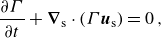 \begin{equation} \frac {\partial \Gamma }{\partial t}+\boldsymbol {\nabla }_{\mathrm {s}}\cdot \left (\Gamma {\boldsymbol {u}}_{\mathrm {s}}\right )=0\,, \end{equation}
where
 ${\boldsymbol {u}}_{\mathrm {s}}$
is the total velocity of the interface, (2.6), which has components both normal and tangential to the interface. The surfactant redistribution gives rise to gradients in the interfacial tension (Marangoni stresses) since the interfacial tension depends on the local surfactant concentration,
${\boldsymbol {u}}_{\mathrm {s}}$
is the total velocity of the interface, (2.6), which has components both normal and tangential to the interface. The surfactant redistribution gives rise to gradients in the interfacial tension (Marangoni stresses) since the interfacial tension depends on the local surfactant concentration,
 $\gamma (\Gamma )$
. Considering small deviations from equilibrium, the equation of state is linearized
$\gamma (\Gamma )$
. Considering small deviations from equilibrium, the equation of state is linearized
 \begin{equation} \gamma (\Gamma )=\gamma _{\mathrm {eq}}(1-E\bar \Gamma )\,, \end{equation}
where
 $\bar \Gamma ={(\Gamma -\Gamma _{\mathrm {eq}})}/{\Gamma _{\mathrm {eq}}}$
and
$\bar \Gamma ={(\Gamma -\Gamma _{\mathrm {eq}})}/{\Gamma _{\mathrm {eq}}}$
and
 $E=-\frac {\Gamma _{\mathrm {eq}}}{\gamma _{\mathrm {eq}}} (\frac {\partial \gamma }{\partial \Gamma } )_{\mathrm {eq}}$
is the elasticity of the monolayer. The interfacial stress balance becomes
$E=-\frac {\Gamma _{\mathrm {eq}}}{\gamma _{\mathrm {eq}}} (\frac {\partial \gamma }{\partial \Gamma } )_{\mathrm {eq}}$
is the elasticity of the monolayer. The interfacial stress balance becomes
 \begin{equation} {{\boldsymbol {\hat {n}}}} \cdot (\boldsymbol {T}^{{\mathrm {out}}}-\boldsymbol {T}^{{\mathrm {ins}}}) = {\textit { Ca}}_{\mathrm {s}}^{-1}\left (1-E\bar {\Gamma }\right ) \left ({\boldsymbol {\nabla }} \cdot {{\boldsymbol {\hat {n}}}} \right ){{\boldsymbol {\hat {n}}}}+ {\textit { Ma}}{\boldsymbol {\nabla }} _{\mathrm {s}}\bar \Gamma \,, \quad \,r=r_{\mathrm {s}}\,. \end{equation}
The capillary number
 ${\textit { Ca}}_{\mathrm {s}}$
is defined relative to the equilibrium interfacial tension
${\textit { Ca}}_{\mathrm {s}}$
is defined relative to the equilibrium interfacial tension
 $\gamma _{\mathrm {eq}}$
. The Marangoni number
$\gamma _{\mathrm {eq}}$
. The Marangoni number
 \begin{equation} {\textit { Ma}}^{-1} = \frac {F}{\Delta \gamma R_0 }={\textit { Ca}}_{\mathrm {s}} E^{-1}\,, \end{equation}
reflects the strength of the Marangoni stresses, which oppose the surfactant redistribution by the flow and act to restore the uniform surfactant coverage. Here,
 $\Delta \gamma =-\Gamma _{\mathrm {eq}} (\frac {\partial \gamma }{\partial \Gamma } )_{\mathrm {eq}}$
is the characteristic magnitude of the Marangoni stresses.
$\Delta \gamma =-\Gamma _{\mathrm {eq}} (\frac {\partial \gamma }{\partial \Gamma } )_{\mathrm {eq}}$
is the characteristic magnitude of the Marangoni stresses.
In the limit
 ${\textit { Ma}}\gg 1$
, the non-uniformities in the surfactant distribution induced by the flow are small,
${\textit { Ma}}\gg 1$
, the non-uniformities in the surfactant distribution induced by the flow are small,
 $\bar \Gamma \sim O({\textit {Ma}}^{-1})$
, and (2.10) reduces to the condition for a surface-incompressible flow (Blawzdziewicz, Vlahovska & Loewenberg Reference Blawzdziewicz, Vlahovska and Loewenberg2000; Vlahovska et al. Reference Vlahovska, Blawzdziewicz and Loewenberg2009)
$\bar \Gamma \sim O({\textit {Ma}}^{-1})$
, and (2.10) reduces to the condition for a surface-incompressible flow (Blawzdziewicz, Vlahovska & Loewenberg Reference Blawzdziewicz, Vlahovska and Loewenberg2000; Vlahovska et al. Reference Vlahovska, Blawzdziewicz and Loewenberg2009)
 \begin{equation} \boldsymbol {\nabla }_{\mathrm {s}}\cdot {\boldsymbol {u}}_{\mathrm {s}}=0\,. \end{equation}
The velocity field is independent of
 $\textit { Ma}$
in this case, as the tension adapts to keep the surface flow area incompressible.
$\textit { Ma}$
in this case, as the tension adapts to keep the surface flow area incompressible.
The active particle swims and it is advected and reoriented by the fluid flow. Its trajectory is given by
 \begin{align} \begin{split} &\frac {d \boldsymbol {{\boldsymbol {x}}_0}}{dt} = \tilde {V}_p {{\boldsymbol {\hat {p}}}}+{\boldsymbol {u}}_p \,\,\quad \frac {d{{\boldsymbol {\hat {p}}}}}{dt} = {\boldsymbol \omega }_p \times {{\boldsymbol {\hat {p}}}} \end{split} ,\end{align}
where the normalized particle velocity is
 $\tilde {V}_p = V_p \mu R_0 /F$
, and
$\tilde {V}_p = V_p \mu R_0 /F$
, and
 ${\boldsymbol {u}}_p, {\boldsymbol \omega }_p$
are the local flow velocity and rotation rate.
${\boldsymbol {u}}_p, {\boldsymbol \omega }_p$
are the local flow velocity and rotation rate.
3. Asymptotic solution for small shape deformation
We solve the problem in the case of weak particle activity, i.e.
 ${\textit { Ca}} \ll 1$
, where the droplet shape remains nearly spherical. Given the spherical geometry of the problem, we expand all variables in spherical harmonics (see Appendix A). Accordingly, the surface in a coordinate system centred at the droplet is parametrized as
${\textit { Ca}} \ll 1$
, where the droplet shape remains nearly spherical. Given the spherical geometry of the problem, we expand all variables in spherical harmonics (see Appendix A). Accordingly, the surface in a coordinate system centred at the droplet is parametrized as
 \begin{equation} r_{\mathrm {s}}(\theta ,\phi ,t) = 1+\epsilon f(\theta ,\phi ,t), \end{equation}
where
 $\epsilon \equiv {\textit { Ca}}$
and the deviation from sphericity is expressed in terms of scalar spherical harmonics
$\epsilon \equiv {\textit { Ca}}$
and the deviation from sphericity is expressed in terms of scalar spherical harmonics
 \begin{equation} f(\theta ,\phi ,t) = \sum _{j=1}^\infty \sum _{m=-j}^{j}f_{jm}(t) y_{jm}(\theta ,\phi ). \end{equation}
Assuming surfactant elasticity
 $E\sim O(1)$
, the surface tension variations are also small (but comparable to the flow stresses)
$E\sim O(1)$
, the surface tension variations are also small (but comparable to the flow stresses)
 \begin{equation} \gamma = \gamma _0+ \epsilon \sum _{j=1}^\infty \sum _{m=-j}^{j} g_{jm}(t)y_{jm}(\theta ,\phi )\,. \end{equation}
3.1. Solution for the fluid velocity
The fluid flows inside and outside the droplet are expanded in a basis of fundamental solutions of the Stokes equation in a spherical geometry,
 ${\boldsymbol {u}}_{jm\sigma }^\pm ({\boldsymbol {x}})$
, where
${\boldsymbol {u}}_{jm\sigma }^\pm ({\boldsymbol {x}})$
, where
 $\pm$
denotes solutions that are regular at infinity
$\pm$
denotes solutions that are regular at infinity
 $(-)$
or at the origin
$(-)$
or at the origin
 $(+)$
, and
$(+)$
, and
 $\sigma =0,1,2$
denote the irrotational, rotational and pressure-conjugate velocity fields (see Appendix A for details).
$\sigma =0,1,2$
denote the irrotational, rotational and pressure-conjugate velocity fields (see Appendix A for details).
The flow velocity inside and outside the droplet is computed in three steps.
-
(i) The flow due to the active particle in free space filled with the droplet fluid, which is the solution
 ${\boldsymbol {u}}({\boldsymbol {x}},{\boldsymbol {x}}_0)$
of (2.4) in a coordinate system centred at the singularity, is expressed in decaying solutions of the Stokes equation(3.4)where
\begin{equation} {\boldsymbol {u}}^{{\mathrm {act}}}({\boldsymbol {x}}) = \sum _{j,m,\sigma } c_{jm\sigma }^{{\mathrm {act}}}{\boldsymbol {u}}_{jm\sigma }^-({\boldsymbol {x}})\,, \end{equation}
$\sum _{j,m,\sigma } = \sum _{j=1}^\infty \sum _{m=-j}^j\sum _{\sigma =0}^2$
. For example a rotlet with axis of rotation
$\boldsymbol {\hat {z}}$
is described by coefficient
$c_{101}^{\mathrm {act}} = -\frac {i}{2\sqrt {6\pi }\lambda }$
.
${\boldsymbol {u}}({\boldsymbol {x}},{\boldsymbol {x}}_0)$
of (2.4) in a coordinate system centred at the singularity, is expressed in decaying solutions of the Stokes equation(3.4)where
\begin{equation} {\boldsymbol {u}}^{{\mathrm {act}}}({\boldsymbol {x}}) = \sum _{j,m,\sigma } c_{jm\sigma }^{{\mathrm {act}}}{\boldsymbol {u}}_{jm\sigma }^-({\boldsymbol {x}})\,, \end{equation}
$\sum _{j,m,\sigma } = \sum _{j=1}^\infty \sum _{m=-j}^j\sum _{\sigma =0}^2$
. For example a rotlet with axis of rotation
$\boldsymbol {\hat {z}}$
is described by coefficient
$c_{101}^{\mathrm {act}} = -\frac {i}{2\sqrt {6\pi }\lambda }$
.
-
(ii) Droplet deformation is computed from (3.1). For this purpose, the flow (3.4) needs to be transformed into a coordinate system centred at the droplet. A similar problem is encountered in the study of electrostatic and gravitational fields, where the field at distant points is sought in terms of sources in a given region, and is solved by the multipole expansion method (Jackson Reference Jackson1999). The difference in our case is that we are dealing with a vector (velocity) not scalar (potential) fields. This problem has been solved by Felderhof & Jones (Reference Felderhof and Jones1989).
The structure of the transformed flow depends on the position
$\boldsymbol {x}$
. In the region
$|{\boldsymbol {x}}|\lt |{\boldsymbol {x}}_0|$
, the velocity field is a superposition of Stokes-flow solutions that are non-singular at the origin. In the region
$|{\boldsymbol {x}}|\gt |{\boldsymbol {x}}_0|$
, the flow consists of Stokes-flow solutions that are non-singular at infinity(3.5)where
\begin{align} {\boldsymbol {u}}^{{\mathrm {act}}}({\boldsymbol {x}},{\boldsymbol {x}}_0) &= \sum _{j,m,\sigma } c_{jm\sigma }^{{\mathrm {act}},+}({\boldsymbol {x}}_0){\boldsymbol {u}}_{jm\sigma }^+({\boldsymbol {x}})H(|{\boldsymbol {x}}_0|-|{\boldsymbol {x}}|)\nonumber \\ &\quad +\,c_{jm\sigma }^{{\mathrm {act}},-}({\boldsymbol {x}}_0)\,,{\boldsymbol {u}}_{jm\sigma }^-({\boldsymbol {x}})H(|{\boldsymbol {x}}|-|{\boldsymbol {x}}_0|) ,\end{align}
$H$
is the step function. The coefficients of the transformed flow
$c_{jm\sigma }^{{\mathrm {act}},\pm }$
are determined by the transformations derived in Felderhof & Jones (Reference Felderhof and Jones1989) and the details are given in Appendix B. Continuing the previous example of the axisymmetric configuration of a rotlet, when the rotlet is placed at
$(x=0,y=0,z=r_0)$
with respect to the drop centre, the coefficients for the expansion are
(3.6)with all other coefficients equal to 0.
\begin{align} c_{j01}^{{\mathrm {act}},-} &=-\frac {i r_0^{j-1}}{4\lambda } \sqrt {\frac {j(j+1)}{(2j+1)\pi }}\,, c_{j02}^{{\mathrm {act}},+} = - \frac {i j r_0^{-j-2}}{4\sqrt {(2j+1)\pi }\lambda }\,,\nonumber\\ c_{j00}^{{\mathrm {act}},+} &=c_{j01}^{{\mathrm {act}},+}= r_0^{-2j-1}c_{j01}^{{\mathrm {act}},-}\,, \end{align}
-
(iii) The total flow is a superposition of the flow due to the singularity and perturbation due to the presence of the interface
(3.7)The above form for the solution satisfies the continuity of velocity at the spherical droplet interface. The unknown coefficients
\begin{align} \begin{split} &{\boldsymbol {u}}^{{\mathrm {ins}}} = {\boldsymbol {u}}^{{\mathrm {act}}}+\sum _{j,m,\sigma } (c_{jm\sigma }-c_{jm\sigma }^{{\mathrm {act}},-}){\boldsymbol {u}}_{jm\sigma }^+\,,\quad {\boldsymbol {u}}^{{\mathrm {out}}} = \sum _{j,m,\sigma } c_{jm\sigma }{\boldsymbol {u}}_{jm\sigma }^-. \end{split} \end{align}
$c_{jm\sigma }$
are determined using the stress balance at the interface. The hydrodynamic tractions associated with the flow are expanded in vector spherical harmonics (Vlahovska Reference Vlahovska2015)(3.8)
\begin{align} \begin{split} &{\textbf {t}} \equiv ({\textbf {T}}^{{\mathrm {ins}}}-{\textbf {T}}^{{\mathrm {out}}}) \cdot {{\boldsymbol {\hat {r}}}} = \sum \tau _{jm\sigma }{{\textbf {y}}}_{jm\sigma }\,,\\ &\tau _{jm\sigma } = \sum _{\sigma '=0}^2 c_{jm\sigma '}T_{\sigma \sigma '}^- - \lambda ((c_{jm\sigma '}-c_{jm\sigma '}^{{\mathrm {act}},-})T_{\sigma \sigma '}^++c_{jm\sigma '}^{{\mathrm {act}},-} T_{\sigma \sigma '}^-)\,, \end{split} \end{align}


where the
 $T_{\sigma \sigma '}^\pm$
are listed in Appendix A.
$T_{\sigma \sigma '}^\pm$
are listed in Appendix A.
Next, we discuss the solution in the case of a surfactant-free drop where the hydrodynamic tractions are balanced by the surface tension only and surfactant-covered drop where the surface traction also include the Marangoni stresses.
3.1.1. Clean droplet
For a surfactant-free droplet, the tangential tractions are continuous (
 $\sigma =0,1$
) and the normal tractions(
$\sigma =0,1$
) and the normal tractions(
 $\sigma =2$
) is balanced by surface tension
$\sigma =2$
) is balanced by surface tension
 \begin{equation} \tau _{jm\sigma }= (-2+j(j+1)) f_{jm} \delta _{\sigma ,2} ,\end{equation}
where
 $\delta _{j,k}$
is the Kronecker delta function.
$\delta _{j,k}$
is the Kronecker delta function.
Solving for
 $c_{jm\sigma }$
yields
$c_{jm\sigma }$
yields
 \begin{align} \begin{split} c_{jm1} = \frac {\lambda (2j+1)}{2j+1+(\lambda -1)(j-1)}c_{jm1}^{{\mathrm {act}},-}\,,\quad c_{jmn} = \zeta _j^{-1}\left ( -p_{jmn} f_{jm}+q_{jmn}\right )\ \quad (n=0,2),\\ \end{split} \end{align}
where
 \begin{align} \begin{split} p_{jm0} = \,&3\sqrt {j(j+1)}(j-1)(j+2)\left ((2j+1)+(\lambda -1)(j+1) \right )\\ q_{jm0} =\,& (2j+1)\lambda (3 c_{jm2}^{{\mathrm {act}},-} \sqrt {j (1 + j)} (\lambda -1) \\ &+\, c_{jm0}^{{\mathrm {act}},-}(j(4j^2+6j-1)+\lambda (j+1)(4j^2+2j-3))\\ p_{jm2} =\,&(j-1)j(j+1)(j+2)(2j+1)(\lambda +1)\\ q_{jm2} =\,& (2j+1)\lambda (3c_{jm0}^{{\mathrm {act}},-} \sqrt {j(j+1)} (\lambda -1) \\ &+\, c_{jm2}^{{\mathrm {act}},-} ((4j^3+6j^2-j+3)+\lambda (4j^3+6j^2-j-6))\\ \zeta _j =\,&(2j-1)(2j+1)^2(2j+3)+(\lambda -1)(2j+1)(8j^3+12j^2-2j-9)\\ &+\,2(\lambda -1)^2(j-1)(j+1)(2j^2+4j+3). \end{split} \end{align}
3.1.2. Surfactant-covered droplet
In this case, the surface incompressibility condition (2.14) gives a relation between the amplitudes of the tangential and radial velocity components
 \begin{equation} c_{jm2} = \frac {1}{2}\sqrt {j(j+1)}c_{jm0} .\end{equation}
The stress balance for the surfactant-covered drop is
 \begin{align} \begin{split} \tau _{jm\sigma } = (2 g_{jm} + (-2+j(j+1)) f_{jm})\delta _{s,2}- \sqrt {j(j+1)} g_{jm}\delta _{s,0} \end{split}. \end{align}
Equation (3.12) and the radial component of (3.13) serve to determine the tangential and radial velocities (
 $c_{jm0}$
and
$c_{jm0}$
and
 $c_{jm2}$
coefficients). The tangential
$c_{jm2}$
coefficients). The tangential
 $\sigma =1$
flow (
$\sigma =1$
flow (
 $c_{jm1}$
coefficients) is obtained from the continuity of the tangential
$c_{jm1}$
coefficients) is obtained from the continuity of the tangential
 $jm1$
stress. The
$jm1$
stress. The
 $jm0$
tangential stress component serves to determine the tension distribution
$jm0$
tangential stress component serves to determine the tension distribution
 $g_{jm}$
(Vlahovska Reference Vlahovska2015). The resulting coefficients for the velocity and tension are
$g_{jm}$
(Vlahovska Reference Vlahovska2015). The resulting coefficients for the velocity and tension are
 \begin{align} \begin{split} &c_{jm0} = \frac {2 c_{jm2}}{\sqrt {j(j+1)}}\,,\quad c_{jm1}= \frac {\lambda (2j+1)}{2j+1+(\lambda -1)(j-1)}c_{jm1}^{{\mathrm {act}},-}\\ & c_{jm2}=\xi _j^{-1}\left ( -p_{jm2} f_{jm}+q_{jm2}\right ) \,,\quad g_{jm} =\xi _j^{-1}\left (-p_{jmg} f_{jm}+q_{jmg} \right )\\ \end{split} \end{align}
where
 \begin{align} \begin{split} p_{jm2} &=(j-1)j(j+1)(j+2)\\ q_{jm2}&= (2j+1)\lambda (\sqrt {j(j+1)}c_{jm0}^{{\mathrm {act}},-}+(2j^2+2j-3)c_{jm2}^{{\mathrm {act}},-})\\ p_{jmg} &=(j-1)(j+2)\left ((2j+1)+(\lambda -1)(j-1)\right )\\ q_{jmg} &=-(2j+1)\lambda \left [ \frac {(2j-1)(2j+1)(2j+3)+(\lambda -1)(j-1)(4j^2+10j+9)}{\sqrt {j(j+1)}}c_{jm0}^{{\mathrm {act}},-} \right. \\ &\quad \left. -\frac {2(2j-1)(2j+1)(2j+3)+(j-1)(8j^2+17j+12)}{j(j+1)}c_{jm2}^{{\mathrm {act}},-}\right ]\\ \xi _j &= (2j+1)(2j^2+2j-1)+(\lambda -1)(j-1)(2j^2+5j+5). \end{split} \end{align}
3.2. Interface evolution and steady shape
The evolution equation for the interface (2.5) is (Vlahovska Reference Vlahovska2015)
 \begin{equation} {\textit { Ca}} \frac {d f_{jm}}{dt} = c_{jm2} = - p_{jm2}f_{jm}+q_{jm2}. \end{equation}
For both clean and surfactant-covered droplets, the coefficient
 $p_{jm2}\gt 0$
for all
$p_{jm2}\gt 0$
for all
 $j\gt 1$
indicating that when the singularity is fixed in place with respect to the drop centre the shape modes
$j\gt 1$
indicating that when the singularity is fixed in place with respect to the drop centre the shape modes
 $f_{jm}$
evolve to a steady-state value given by
$f_{jm}$
evolve to a steady-state value given by
 \begin{equation} f_{jm}^{\mathrm {ss}} =\frac {q_{jm2}}{p_{jm2}}. \end{equation}
Inserting the steady shape in the flow coefficients (3.10) recovers the solution for the flow around a non-deformable clean droplet, which would be obtained by setting the normal velocity to the surface
 $c_{jm2}=0$
and the shape deformation
$c_{jm2}=0$
and the shape deformation
 $f_{jm} = 0$
in the tangential stress balance. The flow and motion of a non-deformable surfactant-covered drop is obtained if the steady-state shape amplitudes,
$f_{jm} = 0$
in the tangential stress balance. The flow and motion of a non-deformable surfactant-covered drop is obtained if the steady-state shape amplitudes,
 $f_{jm}$
, are inserted in (3.14) instead.
$f_{jm}$
, are inserted in (3.14) instead.
For a surfactant-free drops at steady state, the flow for modes
 $j\gt 1$
is then given by
$j\gt 1$
is then given by
 \begin{align} \begin{split} &c_{jm0}^{\mathrm {ss}} = \lambda \frac {2j(j+1)c_{jm0}^{{\mathrm {act}},-}-3\sqrt {j(j+1)}c_{jm2}^{{\mathrm {act}},-}}{j(j+1)(\lambda +1)}\,,\\ &c_{jm1}^{\mathrm {ss}} = \frac {\lambda (2j+1)}{2j+1+(\lambda -1)(j-1)}c_{jm1}^{{\mathrm {act}},-}\,,\\ & c_{jm2}^{\mathrm {ss}} = 0. \end{split} \end{align}
The
 $j=1$
flows remain the same as in (3.10).
$j=1$
flows remain the same as in (3.10).
For a surfactant-covered drop at steady state,
 $f_{jm}^{\mathrm {ss}}$
, the flow for
$f_{jm}^{\mathrm {ss}}$
, the flow for
 $j\gt 1$
reduces to
$j\gt 1$
reduces to
 \begin{align} \begin{split} &c_{jm0}^{\mathrm {ss}} = c_{jm2}^{\mathrm {ss}} = 0\,,\\ &c_{jm1}^{\mathrm {ss}} = \frac {\lambda (2j+1)}{2j+1+(\lambda -1)(j-1)}c_{jm1}^{{\mathrm {act}},-}\,, \end{split} \end{align}
matching the flow about a surfactant-covered spherical drop. The tension adapts to keep the surface flow area-incompressible flow. The tension distribution is obtained from the tangential stress balance
 \begin{align} \begin{split} &g_{jm}^{\mathrm {ss}} = (2j+1)\lambda \frac {-2c_{jm0}^{{\mathrm {act}},-} \sqrt {j(j+1)}+3c_{jm2}^{{\mathrm {act}},-}}{j(j+1)}\,. \end{split} \end{align}
The Marangoni stresses counteract the viscous stresses due to the flow components with velocity amplitudes
 $c_{jm0}$
and
$c_{jm0}$
and
 $c_{jm2}$
. If the active particle generates axisymmetric flow,
$c_{jm2}$
. If the active particle generates axisymmetric flow,
 $\rm m=0$
, then
$\rm m=0$
, then
 $c_{jm1}^{{\mathrm {act}},-}=0$
, the interface is completely immobilized and the flow outside the droplet vanishes.
$c_{jm1}^{{\mathrm {act}},-}=0$
, the interface is completely immobilized and the flow outside the droplet vanishes.
3.3. Drop migration
The translational velocity of a drop is defined as the volume average velocity of the fluid inside the drop
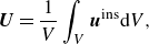 \begin{equation} {\boldsymbol {U}} = \frac {1}{V} \int _V {\boldsymbol {u}}^{{\mathrm {ins}}} {\rm d}V ,\end{equation}
where
 $V$
is the volume of the drop. Under the assumption that the flow is incompressible everywhere,
$V$
is the volume of the drop. Under the assumption that the flow is incompressible everywhere,
 ${\boldsymbol {\nabla }} \cdot {\boldsymbol {u}}^{{\mathrm {ins}}} = 0$
, the following relation holds:
${\boldsymbol {\nabla }} \cdot {\boldsymbol {u}}^{{\mathrm {ins}}} = 0$
, the following relation holds:
 ${\boldsymbol {\nabla }} \cdot ({\boldsymbol {x}}{\boldsymbol {u}}^{{\mathrm {ins}}}) = {\boldsymbol {u}}^{{\mathrm {ins}}}$
. Under the further assumption of the smoothness of
${\boldsymbol {\nabla }} \cdot ({\boldsymbol {x}}{\boldsymbol {u}}^{{\mathrm {ins}}}) = {\boldsymbol {u}}^{{\mathrm {ins}}}$
. Under the further assumption of the smoothness of
 ${\boldsymbol {u}}^{{\mathrm {ins}}}$
, we can relate the drop translation to the surface velocity
${\boldsymbol {u}}^{{\mathrm {ins}}}$
, we can relate the drop translation to the surface velocity
 \begin{equation} {\boldsymbol {U}}= \frac {1}{V} \int _S ({\boldsymbol {u}}^{{\mathrm {ins}}}\cdot {{\boldsymbol {\hat {n}}}}) {\boldsymbol {x}} \rm d\it S ,\end{equation}
where
 $S$
is the surface of the drop. For a spherical drop,
$S$
is the surface of the drop. For a spherical drop,
 ${{\boldsymbol {\hat {n}}}}={{\boldsymbol {x}}} ={{\boldsymbol {\hat {r}}}}$
and
${{\boldsymbol {\hat {n}}}}={{\boldsymbol {x}}} ={{\boldsymbol {\hat {r}}}}$
and
 $V=4\pi /3$
.
$V=4\pi /3$
.
Some care must be taken when placing singularities inside a droplet. Both the incompressibility and smoothness conditions may no longer hold. For a Stokeslet, rotlet, and stresslet, the singularity may be removed in the sense that
 \begin{equation} \int _{V_\delta } {\boldsymbol {u}} dV_{\delta } =O(\delta ) \to 0 \text { as }\delta \to 0 ,\end{equation}
where
 $V_{\delta }$
is a ball of radius
$V_{\delta }$
is a ball of radius
 $\delta$
around the singularity and
$\delta$
around the singularity and
 $\boldsymbol {u}$
is the velocity of the Stokeslet, rotlet or stresslet. This results in definition (3.21) being well defined and relation (3.22) holding.
$\boldsymbol {u}$
is the velocity of the Stokeslet, rotlet or stresslet. This results in definition (3.21) being well defined and relation (3.22) holding.
For higher-order singularities, we have that the volume average velocity as defined in (3.21) does not converge. Note, however, if we were to consider an active particle of finite size with volume
 $V_{active}$
, we have a well defined volume average velocity of the fluid
$V_{active}$
, we have a well defined volume average velocity of the fluid
 \begin{equation} {\boldsymbol {U}} = \frac {1}{V} \int _{V-V_{active}} {\boldsymbol {u}}^{{\mathrm {ins}}} d(V-V_{active}) .\end{equation}
This can be given in terms of surface velocity contributions from the drop surface,
 $S$
, and active particle surface,
$S$
, and active particle surface,
 $S_{AP}$
 \begin{equation} {\boldsymbol {U}}= \frac {1}{V} \int _S ({\boldsymbol {u}}^{{\mathrm {ins}}}\cdot {{\boldsymbol {\hat {n}}}}) {\boldsymbol {x}} {\rm d}S + \frac {1}{V} \int _{S_{AP}} ({\boldsymbol {u}}^{{\mathrm {ins}}}\cdot {{\boldsymbol {\hat {n}}}}_{AP}) {\boldsymbol {x}} {\rm d}S_{AP} ,\end{equation}
where
 ${{\boldsymbol {\hat {n}}}}_{AP}$
is the unit normal vector pointing into the active particle.
${{\boldsymbol {\hat {n}}}}_{AP}$
is the unit normal vector pointing into the active particle.
For the remainder of the paper we will only consider the drop velocity in terms of the contribution from the drop surface and define the velocity of the spherical drop as
 \begin{equation} {\boldsymbol {U}}_{d} = \frac {3}{4\pi } \int _S ({\boldsymbol {u}}_s\cdot {{\boldsymbol {\hat {r}}}}) {{\boldsymbol {\hat {r}}}} dS= \frac {3}{4\pi } \sum _{m=-1}^1 c_{1m2} \int _S {{\textbf {y}}}_{1m2}{\rm d}S. \end{equation}
The integral of the vector spherical harmonic function can be taken on the unit sphere to yield
 \begin{equation} {\boldsymbol {U}}_{d} = \frac {3}{4\pi }\sqrt {\frac {2\pi }{3}}\bigg (c_{1,-1,2}\begin{bmatrix}1\\-i\\0\end{bmatrix}+\sqrt {2}c_{1,0,2}\begin{bmatrix}0\\0\\1\end{bmatrix}+c_{1,1,2}\begin{bmatrix}-1\\-i\\0\end{bmatrix}\bigg ). \end{equation}
For a clean drop, substituting (3.10) for
 $c_{1m2}$
into (3.27), leads to
$c_{1m2}$
into (3.27), leads to
 \begin{equation} {\boldsymbol {U}}_{d}=\frac {\lambda }{2(2+3\lambda )}\sqrt {\frac {3}{2\pi }} \begin{bmatrix}\sqrt {2}(c_{1,-1,0}^{{\mathrm {act}},-}-c_{1,1,0}^{{\mathrm {act}},-})(\lambda -1)+(c_{1,-1,2}^{{\mathrm {act}},-}-c_{1,1,2}^{{\mathrm {act}},-})(\lambda +4) \\[6pt] -i\sqrt {2}(c_{1,-1,0}^{{\mathrm {act}},-}+c_{1,1,0}^{{\mathrm {act}},-})(\lambda -1)-i(c_{1,-1,2}^{{\mathrm {act}},-}+c_{1,1,2}^{{\mathrm {act}},-})(\lambda +4) \\[6pt] 2c_{1,0,0}^{{\mathrm {act}},-}(\lambda -1)+\sqrt {2}c_{1,0,2}^{{\mathrm {act}},-}(\lambda +4) \end{bmatrix}. \end{equation}
The clean drop can only move as a results of singularities that generate the ’
 $1m2$
’ mode when displaced from the origin. A closer inspection of the transforms in Felderhof & Jones (Reference Felderhof and Jones1989) reveals that only linear combinations of the Stokeslet, rotlet, stresslet and source dipole can generate non-zero
$1m2$
’ mode when displaced from the origin. A closer inspection of the transforms in Felderhof & Jones (Reference Felderhof and Jones1989) reveals that only linear combinations of the Stokeslet, rotlet, stresslet and source dipole can generate non-zero
 $c_{1m2}$
coefficient values and thus result in non-zero drop velocity. Higher-order singularities do not induce droplet translation.
$c_{1m2}$
coefficient values and thus result in non-zero drop velocity. Higher-order singularities do not induce droplet translation.
For a surfactant-covered drop, substituting (3.14) into (3.27), yields for the drop velocity
 \begin{equation} {\boldsymbol {U}}_{d} = \frac {\lambda }{3\sqrt {6\pi }}\begin{bmatrix} \sqrt {2}(c_{1,-1,0}^{{\mathrm {act}},-}-c_{1,1,0}^{{\mathrm {act}},-})+c_{1,-1,2}^{{\mathrm {act}},-}-c_{1,1,2}^{{\mathrm {act}},-}\\[6pt] -i(\sqrt {2}(c_{1,-1,0}^{{\mathrm {act}},-}+c_{1,1,0}^{{\mathrm {act}},-})+c_{1,-1,2}^{{\mathrm {act}},-}+c_{1,1,2}^{{\mathrm {act}},-}\\[6pt] \sqrt {2}c_{1,0,0}^{{\mathrm {act}},-}+c_{1,0,2}^{{\mathrm {act}},-} \end{bmatrix} .\end{equation}
Although there are four types of singularities that can produce non-zero
 $c_{1m2}$
coefficients, we will see in the next section that only the Stokeslet can produce a non-zero migration for the surfactant-covered drop.
$c_{1m2}$
coefficients, we will see in the next section that only the Stokeslet can produce a non-zero migration for the surfactant-covered drop.
An alternative approach to calculate the drop velocity is from the force on the droplet divided by the droplet drag coefficient (Sprenger et al. Reference Sprenger, Shaik, Ardekani, Lisicki, Mathijssen, Guzmán-Lastra, Löwen, Menzel and Daddi-Moussa-Ider2020). The result is the same as the one obtained from (3.26) in the case of a spherical drop. However, for a droplet enclosing a Stokeslet (Sprenger et al. Reference Sprenger, Shaik, Ardekani, Lisicki, Mathijssen, Guzmán-Lastra, Löwen, Menzel and Daddi-Moussa-Ider2020) overlooked the contribution of the Stokeslet in the net force on the droplet, and their expression for the drop velocity differs from ours and (Kree et al. Reference Kree, Rueckert and Zippelius2021), see Appendix C for a discussion of this issue.
3.4. Trajectory of the active particle
The flow generated in response to the internal singularity advects the active particle. The resulting trajectory is
 \begin{align} \begin{split} &\frac {d {\boldsymbol {x}}_0}{dt} = \tilde {V}_p \boldsymbol {\hat {p}}+\sum _{j,m,\sigma } (c_{jm\sigma }-c_{jm\sigma }^{{\mathrm {act}},-}){\boldsymbol {u}}_{jm\sigma }^+\\ &\frac {d\boldsymbol {\hat {p}}}{dt} = \frac {1}{2}\left ( \sum _{j,m,\sigma } (c_{jm\sigma }-c_{jm\sigma }^{{\mathrm {act}},-}){\boldsymbol {\nabla }} \times {\boldsymbol {u}}_{jm\sigma }^+\right )\times \boldsymbol {\hat {p}}. \end{split} \end{align}
4. Results and discussion
Here, we discuss the flows generated and the drop migration induced by a Stokeslet, rotlet and axisymmetric force dipole. Notable results for higher-order singularities are also given. We show that transient shape deformation has a significant impact on the particle trajectory.
4.1. Stokeslet
The flow due to a point force in the direction
 ${{\boldsymbol {\hat {\rm d}}}} = ({\rm d}_x,{\rm d}_y,{\rm d}_z)$
in the coordinate system centred at the singularity is given by coefficients
${{\boldsymbol {\hat {\rm d}}}} = ({\rm d}_x,{\rm d}_y,{\rm d}_z)$
in the coordinate system centred at the singularity is given by coefficients
 \begin{align} \begin{split} c_{1,-1,0}^{{\mathrm {act}}} = \frac {{\rm d}_x+i {\rm d}_y}{4\sqrt {3\pi }\lambda }, \,\, c_{1,0,0}^{{\mathrm {act}}} = \frac {{\rm d}_z}{2\sqrt {6\pi }\lambda }, \,\, c_{1,1,0}^{{\mathrm {act}}} = -\frac {{\rm d}_x-i {\rm d}_y}{4\sqrt {3\pi }\lambda }\\[4pt] c_{1,-1,2}^{{\mathrm {act}}} = \frac {{\rm d}_x+i {\rm d}_y}{2\sqrt {6\pi }\lambda }, \,\, c_{1,0,2}^{{\mathrm {act}}} = \frac {{\rm d}_z}{2\sqrt {3\pi }\lambda }, \,\, c_{1,1,2}^{{\mathrm {act}}} = -\frac {{\rm d}_x-i {\rm d}_y}{2\sqrt {6\pi }\lambda }. \end{split} \end{align}
Upon using the transforms in Felderhof & Jones (Reference Felderhof and Jones1989), the coefficients for the flow in the coordinate system centred at the drop are obtained (see Appendix B for details)
 \begin{align} \begin{split} c_{jm0}^{{\mathrm {act}},-} &=\frac {r_0 ^{j-1}}{2(2j+1)\lambda }\left [-\frac {(j-2)({\rm d}_{jm2}\sqrt {j(j+1)}+{\rm d}_{jm0}(j+1))}{2j-1}\right. \\ &\quad \left. +\frac {j({\rm d}_{jm2}\sqrt {j(j+1)}+{\rm d}_{jm0}(j+3))}{2j+3}r_0 ^2\right ]\\ c_{jm1}^{{\mathrm {act}},-} &=\frac {r_0 ^j}{(2j+1)\lambda }{\rm d}_{jm1}\\ c_{jm2}^{{\mathrm {act}},-} &=\frac {r_0 ^{j-1}}{2(2j+1)\lambda }\left [\frac {(j+1)({\rm d}_{jm2}j+d_{jm0}\sqrt {j(j+1)})}{2j-1}\right. \\ &\quad \left. -\frac {({\rm d}_{jm2}j(j+1)+{\rm d}_{jm0}\sqrt {j(j+1)}(j+3))}{2j+3}r_0 ^2\right ]\\ \end{split} \end{align}
 \begin{align} \begin{split} c_{jm0}^{{\mathrm {act}},+} &=\frac {r_0^{-j}}{2(2j+1)\lambda }\left [\frac {(j+1)({\rm d}_{jm2}\sqrt {j(j+1)}-{\rm d}_{jm0}(j-2))}{2j-1}\right. \\ &\quad \left. -\frac {(j+3)({\rm d}_{jm2}\sqrt {j(j+1)}-{\rm d}_{jm0}j)}{2j+3}r_0^{-2}\right ]\\ c_{jm1}^{{\mathrm {act}},+} &=\frac {r_0^{-j-1}}{(2j+1)\lambda }{\rm d}_{jm1}\\ c_{jm2}^{{\mathrm {act}},+} &=\frac {r_0^{-j}}{2(2j+1)\lambda }\left [\frac {{\rm d}_{jm2}j(j+1)-{\rm d}_{jm0}\sqrt {j(j+1)}(j-2)}{2j-1}\right. \\ &\quad \left. +\frac {j(-{\rm d}_{jm2}(j+1)+{\rm d}_{jm0}\sqrt {j(j+1)}}{2j+3}r_0^{-2}\right ], \end{split}\end{align}
where the singularity is located at
 ${\boldsymbol {x}}_0 = (r_0,\theta _0,\phi _0)$
in spherical coordinates and
${\boldsymbol {x}}_0 = (r_0,\theta _0,\phi _0)$
in spherical coordinates and
 ${\rm d}_{jm\sigma } = {{\boldsymbol {\hat {d}}}} \cdot {{\textbf {y}}}_{jm\sigma }^\ast (\theta _0,\phi _0)$
. The expressions above have been simplified and are not valid for
${\rm d}_{jm\sigma } = {{\boldsymbol {\hat {d}}}} \cdot {{\textbf {y}}}_{jm\sigma }^\ast (\theta _0,\phi _0)$
. The expressions above have been simplified and are not valid for
 $\theta _0=0,\pi$
as a result. The full expressions listed in Appendix B.3 should be used to evaluate the coefficients for
$\theta _0=0,\pi$
as a result. The full expressions listed in Appendix B.3 should be used to evaluate the coefficients for
 $\theta _0=0,\pi$
.
$\theta _0=0,\pi$
.
4.1.1. Stokeslet in a surfactant-free droplet
Substituting (4.3) into (3.10) and (3.11) gives the coefficients for the flow accounting for the confining interface
 \begin{equation} c_{jm1} = \zeta _j^{-1}\left (\frac {r_0^{j} {\rm d}_{jm1}}{2j+1+(\lambda -1)(j-1)}\right ),\!\!\quad c_{jmn} = \zeta _j^{-1}\left ( -p_{jmn}f_{jm}+q_{jmn}\right )\!\!\quad (n=0,2)\\ \end{equation}
where
 \begin{align} \begin{split} q_{jm0} &= \frac {r_0^{j-1}}{2}\left [{\rm d}_{jm0}\left ((2j+1)\left (-(j-2)(j+1)(2j+3)+j(j+3)(2j-1)r_0^2\right )\right. \right. \\ &\quad \left. +2(\lambda -1)(j+1)\left (-(j+1)(j^2-j-3)+(j-1)j(j+3)r_0^2\right )\right )\\ &\quad +{\rm d}_{jm2} \sqrt {j(j+1)}\left ((2j+1)\left (-(j-2)(2j+3)+j(2j-1)r_0^2\right )\right. \\ &\quad \left. \left. +2(\lambda -1)(j+1)\left (-j^2+j+3+(j-1)j r_0^2\right )\right )\right ]\\ q_{jm2} &= -\frac {r_0^{j-1}}{2}\left [ {\rm d}_{jm0}\sqrt {j(j+1)}\left ((2j+1)\left (-(j+1)(2j+3)+(j+3)(2j-1)r_0^2\right )\right. \right. \\ &\quad \left. +2(\lambda -1)(j+1)\left (-j(j+2)+(j-1)(j+3)r_0^2\right ) \right )\\ &\quad +{\rm d}_{jm2}j(j+1)\left ((2j+1)\left (-(2j+3)+(2j-1)r_0^2\right )\right. \\ &\quad \left. \left. +2(\lambda -1)\left (-j(j+2)+(j-1)(j+1)r_0^2\right ) \right )\right ] \end{split} \end{align}
and
 $\zeta _j$
,
$\zeta _j$
,
 $p_{jm0}$
and
$p_{jm0}$
and
 $p_{jm2}$
are provided in (3.11).
$p_{jm2}$
are provided in (3.11).
The steady-state shape of a drop with a Stokeslet at a fixed position with respect to the centre of the drop is
 \begin{align} \begin{split} f^{\mathrm {ss}}_{jm} &= \frac {q_{jm2}}{p_{jm2}}, \,\, j\geqslant 2 . \end{split} \end{align}
Asymptotically for large
 $j$
,
$j$
,
 $f_{jm}^{\mathrm {ss}} \sim r_0^{j-1} j^{-1}$
. For a Stokeslet near the centre of the particle, the amplitude of the shape mode decay is a power law,
$f_{jm}^{\mathrm {ss}} \sim r_0^{j-1} j^{-1}$
. For a Stokeslet near the centre of the particle, the amplitude of the shape mode decay is a power law,
 $r_0^{j-1}$
, while for a Stokeslet closer to the boundary, the amplitudes decay is dominated by the
$r_0^{j-1}$
, while for a Stokeslet closer to the boundary, the amplitudes decay is dominated by the
 $1/j$
factor.
$1/j$
factor.
In general, the droplet migration velocity depends on the instantaneous shape. However, at steady state, (4.4), (4.6) and (3.28) yield
 \begin{equation} {\boldsymbol {U}}_{d} = \frac {1}{4\pi (2+3\lambda )}\left[(2\lambda +3){{\boldsymbol {\hat {d}}}}+r_0^2(-2{{\boldsymbol {\hat {d}}}}+({{\boldsymbol {\hat {d}}}}\cdot {{\boldsymbol {\hat {r}}}}){{\boldsymbol {\hat {r}}}}) \right]. \end{equation}
The direction of drop translation is in general misaligned with the direction of the point force of the Stokeslet; the correction is proportional to the off-centre location of the singularity,
 $r_0$
. The droplet velocity becomes the same as the Hadamard–Rybczynski expression when the Stokeslet is on the droplet surface,
$r_0$
. The droplet velocity becomes the same as the Hadamard–Rybczynski expression when the Stokeslet is on the droplet surface,
 $r_0=1$
and
$r_0=1$
and
 ${{\boldsymbol {\hat {d}}}}={{\boldsymbol {\hat {r}}}}$
. The results for the steady flow and velocity of the drop agree with those derived in Kree et al. (Reference Kree, Rueckert and Zippelius2021) for non-deformable droplets.
${{\boldsymbol {\hat {d}}}}={{\boldsymbol {\hat {r}}}}$
. The results for the steady flow and velocity of the drop agree with those derived in Kree et al. (Reference Kree, Rueckert and Zippelius2021) for non-deformable droplets.

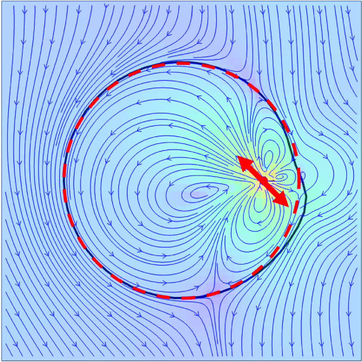
Figure 2. Stokeslet inside a droplet with clean interface,
 ${Ca}=.5, \lambda =1$
. The steady flow and drop shape contour in the equatorial plane
${Ca}=.5, \lambda =1$
. The steady flow and drop shape contour in the equatorial plane
 $z=0$
. The stokeslet is located at
$z=0$
. The stokeslet is located at
 $(.7,0,0)$
with different orientations (a)
$(.7,0,0)$
with different orientations (a)
 ${{\boldsymbol {\hat {d}}}} = (-1,0,0)$
, (b)
${{\boldsymbol {\hat {d}}}} = (-1,0,0)$
, (b)
 ${{\boldsymbol {\hat {d}}}} = (-1/\sqrt (2),1/\sqrt (2),0)$
, (c)
${{\boldsymbol {\hat {d}}}} = (-1/\sqrt (2),1/\sqrt (2),0)$
, (c)
 ${{\boldsymbol {\hat {d}}}} = (0,1,0)$
. Flows are given in the frame of reference moving with the droplet and the colour indicates the magnitude of the velocity. The dashed line outlines the undeformed droplet contour.
${{\boldsymbol {\hat {d}}}} = (0,1,0)$
. Flows are given in the frame of reference moving with the droplet and the colour indicates the magnitude of the velocity. The dashed line outlines the undeformed droplet contour.
Figure 2 shows the flow and steady shape of the interface for several configurations of the Stokeslet inside the surfactant-free droplet. The interface of the drop is depressed inwards behind the Stokeslet and inflated outwards in front of it due to the Stokeslet pulling in fluid from behind and pushing it forward. The confinement leads to the circulation of the flow inside the drop. If the Stokeslet direction is aligned with the line connecting the droplet centre and the singularity location, this line of centres is a symmetry axis and drop migration is in the same direction as the point force. If the Stokeslet is perpendicular to the line of centre, droplet velocity is still colinear with the point force but smaller than the previous axisymmetric configuration.
4.1.2. Stokeslet in a surfactant-covered droplet
For a surfactant-covered drop, the velocity coefficients are obtained by substituting (4.3) into (3.14) and (3.15)
 \begin{align} \begin{split} &c_{jm0} = \frac {2c_{jm2}}{\sqrt {j(j+1)}} \,,\quad c_{jm1} = \frac {r_0 ^{j} {\rm d}_{jm1}}{j+2+\lambda (j-1)}\,,\\ & c_{jm2} =\xi _j^{-1}\left ( -p_{jm2} f_{jm}+q_{jm2}\right )\,,\quad g_{jm} = \xi _j^{-1}\left (-p_{jmg} f_{jm}+q_{jmg}\right )\,, \\ \end{split} \end{align}
where
 \begin{align} \begin{split} q_{jm2} &=-\frac {r_0 ^{j-1}}{2}\left ({\rm d}_{jm0}\sqrt {j(j+1)}(j-1)(-(j+1)+(j+3)r_0^2)\right. \\ &\quad \left. +\,{\rm d}_{jm2} j(j+1)(-(j+1)+(j-1)r_0^2)\right )\\ q_{jmg} &= -\frac {r_0^{j-1}}{2}\left [\frac { {\rm d}_{jm0}}{\sqrt {j(j+1)}}\left ((2j+1)\left (-j(j+1)(2j+3)+(j+2)(j+3)(2j-1)r_0^2\right )\right. \right. \\ &\quad \left. +2(\lambda -1)(j-1)(j+1)\left (-(j^2+3j+3)+(j+2)(j+3)r_0^2 \right )\right )\\ &\quad +{\rm d}_{jm2}\left ((2j+1)\left (-j(2j+3)+(j+2)(2j-1)r_0^2\right )\right.\\ &\quad\left. \left. +2(\lambda -1)(j-1)(-(j^2+3j+3)+(j+1)(j+2)r_0^2)\right )\right ] \end{split} \end{align}
and
 $p_{jm2}$
,
$p_{jm2}$
,
 $p_{jmg}$
and
$p_{jmg}$
and
 $\xi _j$
are given in (3.15).
$\xi _j$
are given in (3.15).
The steady-state droplet shape is described by the shape mode amplitudes
 \begin{align} \begin{split} f_{jm}^{\mathrm {ss}} &=-\frac {r_0 ^{j-1}}{2(j-1)j(j+1)(j+2)}\left [{\rm d}_{jm0}\sqrt {j(j+1)}(j-1)(-(j+1)+(j+3)r_0^2)\right. \\ &\quad \left. +{\rm d}_{jm2} j(j+1)(-(j+1)+(j-1)r_0^2)\right ], \,\, j\geqslant 2. \end{split} \end{align}
Asymptotically for large
 $j$
, the amplitudes of the shape modes decay as
$j$
, the amplitudes of the shape modes decay as
 $f_{jm}^{\mathrm {ss}} \sim r_0 ^{j-1} j^{-1}$
, obeying the same general behaviour as the clean drop case.
$f_{jm}^{\mathrm {ss}} \sim r_0 ^{j-1} j^{-1}$
, obeying the same general behaviour as the clean drop case.
Evaluating (3.29) with (4.8) and (4.10), shows that the drop velocity at steady state is
 \begin{equation} {\boldsymbol {U}}_{d}^{{\mathrm {surfactant}}} = \frac {1}{6\pi } {{\boldsymbol {\hat {d}}}}\,. \end{equation}
Independent of the location of the Stokeslet inside the drop and the
 $\textit { Ma}$
, the migration of the drop is the same as a solid particle experiencing a force with direction
$\textit { Ma}$
, the migration of the drop is the same as a solid particle experiencing a force with direction
 ${\boldsymbol {\hat {d}}}$
at its centre. The surfactant redistribution by the Stokeslet flow generates Marangoni stresses that in the limit of surfactant-incompressible flow (
${\boldsymbol {\hat {d}}}$
at its centre. The surfactant redistribution by the Stokeslet flow generates Marangoni stresses that in the limit of surfactant-incompressible flow (
 ${\textit { Ma}}\rightarrow \infty$
) suppress streaming flows for which
${\textit { Ma}}\rightarrow \infty$
) suppress streaming flows for which
 $\nabla _s\cdot {\boldsymbol {u}}_{\mathrm {s}}\ne 0$
. Thus the interface is effectively rigid (although there can be recirculating surface flows of the ’jm1’ type that are solenoidal, like rigid body rotation described by the ’1m1’ velocity field). The flows and steady shapes for the surfactant-covered droplet are qualitatively similar to the flows and steady shape for surfactant-free droplets shown in figure 2.
$\nabla _s\cdot {\boldsymbol {u}}_{\mathrm {s}}\ne 0$
. Thus the interface is effectively rigid (although there can be recirculating surface flows of the ’jm1’ type that are solenoidal, like rigid body rotation described by the ’1m1’ velocity field). The flows and steady shapes for the surfactant-covered droplet are qualitatively similar to the flows and steady shape for surfactant-free droplets shown in figure 2.
4.2. Rotlet
The flow due to a particle spinning in unbounded Stokes flow is given by the rotlet. The coefficients for the rotlet in a coordinate system centred about itself is given by
 \begin{equation} c_{1,-1,1}^{{\mathrm {act}}} = \frac {-i{\rm d}_x+{\rm d}_y}{4\sqrt {3\pi }\lambda }, \,\, c_{1,0,1}^{{\mathrm {act}}} = -\frac {i {\rm d}_z}{2\sqrt {6\pi }\lambda }, \,\, c_{1,1,1}^{{\mathrm {act}}} = \frac {i {\rm d}_x+{\rm d}_y}{4\sqrt {3\pi }\lambda }. \end{equation}
The coefficients for the rotlet in a coordinate system centred at the drop is
 \begin{align} \begin{split} &c_{jm0}^{{\mathrm {act}},-} = -\frac {i j r_0^j}{2\lambda (2j+1)}{\rm d}_{jm1},\hspace {20pt}c_{jm2}^{{\mathrm {act}},-} =\frac {i\sqrt {j(j+1)}r_0^j}{2\lambda (2j+1)}{\rm d}_{jm1}\\ &c_{jm1}^{{\mathrm {act}},-} = -\frac {i(j+1)r_0^{j-1}}{2\sqrt {j(j+1)}(2j+1)\lambda }(\sqrt {j(j+1)}{\rm d}_{jm0}+j{\rm d}_{jm2})\\ &c_{jm0}^{{\mathrm {act}},+} = \frac {i(j+1)r_0^{-j-1}}{2\lambda (2j+1)}{\rm d}_{jm1}, \hspace {20pt} c_{jm2}^{{\mathrm {act}},+} = \frac {i\sqrt {j(j+1)}r_0^{-j-1}}{2\lambda (2j+1)}{\rm d}_{jm1}\\ &c_{jm1}^{{\mathrm {act}},+} =\frac {i\sqrt {j(j+1)}r_0^{-j-2}}{2(j+1)(2j+1)\lambda }(\sqrt {j(j+1)}{\rm d}_{jm0}-(j+1){\rm d}_{jm2}). \end{split} \end{align}
Similar to the case of the Stokeslet, the expressions above cannot be evaluated for
 $\theta _0 = 0,\pi$
and the full expressions listed in Appendix B.4 should be used in those cases.
$\theta _0 = 0,\pi$
and the full expressions listed in Appendix B.4 should be used in those cases.
4.2.1. Rotlet in a surfactant-free droplet
For the surfactant-free drop, substituting (4.13) for the rotlet into (3.10) and (3.11) yields the velocity coefficients
 \begin{align} \begin{split} c_{jm0} &=\zeta _j^{-1}\left (-p_{jm0} f_{jm}-\frac {i j(2j+3)r_0 ^j}{2}\left ((2j-1)(2j+1)\right. \right. \\&\quad \left.\left. +\,2(\lambda -1)(j-1)(j+1)\right ){\rm d}_{jm1}\right )\\ c_{jm1} &= -\frac {i(j+1)r_0^{j-1}}{2\sqrt {j(j+1)}(2j+1+(\lambda -1)(j-1))}(\sqrt {j(j+1)}d_{jm0}+j d_{jm2})\\ c_{jm2} &=\zeta _j^{-1}\left ( -p_{jm2}f_{jm}+\frac {i\sqrt {j(j+1)}(2j+3)r_0^j}{2}\left ((2j-1)(2j+1)\right. \right. \\ &\quad \left. \left. +2(\lambda -1)(j-1)(j+1)\right ){\rm d}_{jm1}\right ), \end{split} \end{align}
where
 $p_{jm0},p_{jm2},\zeta _j$
are given in (3.11).
$p_{jm0},p_{jm2},\zeta _j$
are given in (3.11).
The steady shape for a droplet with a rotlet fixed in place with respect to the drop centre is
 \begin{equation} f_{jm}^{\mathrm {ss}} = \frac {i r_0^j\sqrt {j(j+1)}(2j+3)\left ((2j-1)(2j+1)+2(\lambda -1)(j-1)(j+1)\right )}{2(j-1)j(j+1)(j+2)(\lambda +1)}{\rm d}_{jm1}, \,\, j\geqslant 2. \end{equation}
Asymptotically for large
 $j$
, the shape modes decay as
$j$
, the shape modes decay as
 $f_{jm}^{\mathrm {ss}} \sim r_0^j$
.
$f_{jm}^{\mathrm {ss}} \sim r_0^j$
.
Substituting (4.14) into (3.28), the steady-state velocity of the drop due to the rotlet is
 \begin{equation} {\boldsymbol {U}}_{d} = -\frac {5r_0}{8\pi (2+3\lambda )}{{\boldsymbol {\hat {d}}}}\times {{\boldsymbol {\hat {r}}}} .\end{equation}
An enclosed rotlet can only drive net motion of the drop if its axis of rotation does not point directly towards or away from the centre of the drop. The velocity of the drop also scales linearly with the distance of the rotlet from the centre of the drop with the direction of motion directed perpendicular to the axis of rotation of the rotlet and the line containing the singularity location and drop centre. A rotlet located in the centre of a drop does not induce any drop migration. Equation (4.16) agrees with the velocity for a rotlet in a drop that can be derived from force dipole results given in Kree et al. (Reference Kree, Rueckert and Zippelius2021).
An example of the flow induced by a rotlet inside a clean drop is shown in figure 3(a). The axis of rotation of the rotlet is
 $\boldsymbol {\hat {z}}$
. and it is spinning counterclockwise in the view of the equatorial plane,
$\boldsymbol {\hat {z}}$
. and it is spinning counterclockwise in the view of the equatorial plane,
 $z=0$
. Both a depression and inflation of the interface is seen near the rotlet and the singularity induces drop migration in the negative y-direction.
$z=0$
. Both a depression and inflation of the interface is seen near the rotlet and the singularity induces drop migration in the negative y-direction.

Figure 3. Rotlet inside a droplet,
 ${Ca} =.5, {\lambda }=1$
. The steady flow and droplet contour in the equatorial plane
${Ca} =.5, {\lambda }=1$
. The steady flow and droplet contour in the equatorial plane
 $z=0$
due to a rotlet placed at
$z=0$
due to a rotlet placed at
 $(.7,0,0)$
with orientation
$(.7,0,0)$
with orientation
 ${{\boldsymbol {\hat {d}}}} = (0,0,1)$
inside (a) a clean droplet and (b) a surfactant-covered droplet. Flows are in the frame of reference moving with the droplet and the colour scheme indicates the magnitude of the velocity. The dashed line outlines the undeformed droplet contour.
${{\boldsymbol {\hat {d}}}} = (0,0,1)$
inside (a) a clean droplet and (b) a surfactant-covered droplet. Flows are in the frame of reference moving with the droplet and the colour scheme indicates the magnitude of the velocity. The dashed line outlines the undeformed droplet contour.
4.2.2. Rotlet in a surfactant-covered drop
For the surfactant-covered drop, substituting (4.13) into (3.14) and (3.15) yields the following velocity coefficients and tension distribution:
 \begin{align} \begin{split} c_{jm0} &= \frac {2c_{jm2}}{\sqrt {j(j+1)}}\\ c_{jm1} &= -\frac {i(j+1)r_0^{j-1}}{2\sqrt {j(j+1)}(2j+1+(\lambda -1)(j-1))}(\sqrt {j(j+1)}{\rm d}_{jm0}+j {\rm d}_{jm2})\\ c_{jm2}&= \xi _j^{-1}\left (-p_{jm2}f_{jm}+\frac {1}{2}i\sqrt {j(j+1)}(j-1)(2j+3)r_0^j {\rm d}_{jm1}\right )\\ g_{jm} &= \xi _j^{-1}\left (-p_{jmg}f_{jm}+\frac {i(j+2)(2j+3)}{2\sqrt {j(j+1)}}\left ((2j-1)(2j+1)\right. \right. \\&\quad \left. \left. +\,2(\lambda -1)(j-1)(j+1) \right )r_0^j{\rm d}_{jm1}\right ), \end{split} \end{align}
where
 $p_{jm2},p_{jmg},\xi _j$
are given in (3.15).
$p_{jm2},p_{jmg},\xi _j$
are given in (3.15).
For a surfactant-covered drop containing a rotlet fixed in place with respect to the centre of the drop, the steady shape is
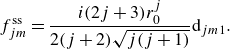 \begin{equation} f_{jm}^{\mathrm {ss}} = \frac {i(2j+3)r_0^j}{2(j+2)\sqrt {j(j+1)}}{\rm d}_{jm1}. \end{equation}
Asymptotically for large
 $j$
, the amplitude of the shape modes is
$j$
, the amplitude of the shape modes is
 $f_{jm}^{\mathrm {ss}} \sim r_0^j /j$
. This differs by a factor of
$f_{jm}^{\mathrm {ss}} \sim r_0^j /j$
. This differs by a factor of
 $j^{-1}$
from the case of the clean drop, with the difference becoming more pronounced as the rotlet moves closer to the surface, i.e.
$j^{-1}$
from the case of the clean drop, with the difference becoming more pronounced as the rotlet moves closer to the surface, i.e.
 $r_0 \to 1$
. Substituting (4.17) into (3.28) reveals that the surfactant suppresses translational drop motion.
$r_0 \to 1$
. Substituting (4.17) into (3.28) reveals that the surfactant suppresses translational drop motion.
Figure 3(b) shows the flow induced by a rotlet in a steady shape surfactant-covered drop in the frame of reference moving with the drop. Although the shape is similar to the clean drop with an enclosed rotlet in the same position, the flow around the surfactant-covered droplet does not contain any translational component associated with the
 $j=1$
modes.
$j=1$
modes.
4.3. Axisymmetric stresslet
The flow due to the axisymmetric stresslet is given by
 \begin{equation} {\boldsymbol {u}}^{{\mathrm {act}}}({\boldsymbol {x}}) = \frac {P}{8\pi \lambda |{\boldsymbol {x}}|^2}\left (-\frac {{\boldsymbol {x}}}{|{\boldsymbol {x}}|}+3\frac {({{\boldsymbol {\hat {d}}}}\cdot {\boldsymbol {x}})^2{\boldsymbol {x}}}{|{\boldsymbol {x}}|^3}\right ) ,\end{equation}
where
 $P = \pm 1$
.
$P = \pm 1$
.
 $P=1$
corresponds to the flow produced by a pusher that expels fluid along
$P=1$
corresponds to the flow produced by a pusher that expels fluid along
 ${\boldsymbol {\hat {d}}}$
and
${\boldsymbol {\hat {d}}}$
and
 $P=-1$
corresponds to the flow of produced by a puller that expel fluid perpendicular to
$P=-1$
corresponds to the flow of produced by a puller that expel fluid perpendicular to
 ${\boldsymbol {\hat {d}}}$
(Lauga Reference Lauga2016; Saintillan Reference Saintillan2018; Lauga Reference Lauga2020). The coefficients for an axisymmetric stresslet in a coordinate system centred at itself is
${\boldsymbol {\hat {d}}}$
(Lauga Reference Lauga2016; Saintillan Reference Saintillan2018; Lauga Reference Lauga2020). The coefficients for an axisymmetric stresslet in a coordinate system centred at itself is
 \begin{align} \begin{split} c_{2,-2,2}^{{\mathrm {act}}} &= \frac {P}{4\lambda }\sqrt {\frac {3}{10\pi }}({\rm d}_x+i {\rm d}_y)^2, c_{2,-1,2}^{{\mathrm {act}}} = \frac {P}{2\lambda }\sqrt {\frac {3}{10\pi }}({\rm d}_x+i {\rm d}_y){\rm d}_z,\\ c_{2,0,2}^{{\mathrm {act}}} &= \frac {P}{4\lambda \sqrt {5\pi }}(1-3 d_z^2), c_{2,1,2}^{{\mathrm {act}}} = \frac {P}{2\lambda }\sqrt {\frac {3}{10\pi }}({\rm d}_x-i {\rm d}_y){\rm d}_z, \\ c_{2,2,2}^{{\mathrm {act}}} &= \frac {P}{4\lambda }\sqrt {\frac {3}{10\pi }}({\rm d}_x-i {\rm d}_y)^2. \end{split} \end{align}
The expression for the flow coefficients of the axisymmetric stresslet and the droplet shape are listed in Appendix B.5. We observe that the shape coefficients decay as
 $r_0^{j-2}$
, slower that the shape modes excited by the Stokeslet and rotlet. Thus for the same
$r_0^{j-2}$
, slower that the shape modes excited by the Stokeslet and rotlet. Thus for the same
 $\textit { Ca}$
, the droplet deformation due to the stresslet is more pronounced.
$\textit { Ca}$
, the droplet deformation due to the stresslet is more pronounced.

Figure 4. Axisymmetric stresslet inside a clean droplet,
 ${Ca}=.2, {\lambda =1}$
. Flow and drop shape in response to a axisymmetric stresslet located at
${Ca}=.2, {\lambda =1}$
. Flow and drop shape in response to a axisymmetric stresslet located at
 $(.7,0,0)$
with different orientations (a)
$(.7,0,0)$
with different orientations (a)
 ${{\boldsymbol {\hat {d}}}} = (-1,0,0)$
, (b)
${{\boldsymbol {\hat {d}}}} = (-1,0,0)$
, (b)
 ${{\boldsymbol {\hat {d}}}} = (-1/\sqrt (2),1/\sqrt (2),0)$
, (c)
${{\boldsymbol {\hat {d}}}} = (-1/\sqrt (2),1/\sqrt (2),0)$
, (c)
 ${{\boldsymbol {\hat {d}}}} = (0,1,0)$
. Flows are in the frame of reference moving with the droplet and the colour scheme indicates magnitude of the velocity.
${{\boldsymbol {\hat {d}}}} = (0,1,0)$
. Flows are in the frame of reference moving with the droplet and the colour scheme indicates magnitude of the velocity.
Using (3.28) for the clean drop and the coefficients for the flow due to confinement, obtained by substituing the results in Appendix B.5 into (3.10) and (3.11), the droplet velocity induced by an axisymmetric stresslet located at
 ${\boldsymbol {x}}_0$
is
${\boldsymbol {x}}_0$
is
 \begin{equation} {\boldsymbol {U}}_{d} = \frac {P r_0}{4\pi (2+3\lambda )}({{\boldsymbol {\hat {r}}}}-3({{\boldsymbol {\hat {d}}}} \cdot {{\boldsymbol {\hat {r}}}}){{\boldsymbol {\hat {d}}}}). \end{equation}
The drop velocity scales linearily with the distance of the stresslet from the centre of the drop. A stresslet at the centre of a drop does not induce drop displacement.
For the surfactant-covered drop, substituting the results in Appendix B.5 into (3.14) and (3.15) to compute the flow coefficients and using (3.29) to compute the drop velocity, shows that drop migration is suppressed.
Figure 4 and figure 5 show the steady shape and flow generated by an axisymmetric stresslet with
 $P=1$
in a clean and a surfactant-covered droplet, respectively, in the frame of reference of the drop. The interface of the drop is bulged along the axis
$P=1$
in a clean and a surfactant-covered droplet, respectively, in the frame of reference of the drop. The interface of the drop is bulged along the axis
 ${\boldsymbol {\hat {d}}}$
of the stresslet and is pulled in perpendicular to it.
${\boldsymbol {\hat {d}}}$
of the stresslet and is pulled in perpendicular to it.
In the case of the surfactant-covered drop, the Marangoni stresses suppress the flow with amplitudes
 $c_{jm0}$
and
$c_{jm0}$
and
 $c_{jm2}$
; only the
$c_{jm2}$
; only the
 $c_{jm1}$
-type flow, which is by definition surface incompressible on a sphere, is transmitted outside the drop. The axisymmetric configuration of the stresslet shown in figure 5(a) does not induce
$c_{jm1}$
-type flow, which is by definition surface incompressible on a sphere, is transmitted outside the drop. The axisymmetric configuration of the stresslet shown in figure 5(a) does not induce
 $c_{jm1}$
flow and thus there is no fluid motion outside of the drop. There is no drop migration for all of the configurations of the stresslet inside of the surfactant-covered drop.
$c_{jm1}$
flow and thus there is no fluid motion outside of the drop. There is no drop migration for all of the configurations of the stresslet inside of the surfactant-covered drop.

Figure 5. Axisymmetric stresslet inside a surfactant-covered droplet,
 ${Ca}=.2, \lambda =1$
. Flow and drop shape in response to a axisymmetric stresslet located at
${Ca}=.2, \lambda =1$
. Flow and drop shape in response to a axisymmetric stresslet located at
 $(.7,0,0)$
with different orientations (a)
$(.7,0,0)$
with different orientations (a)
 ${{\boldsymbol {\hat {d}}}} = (-1,0,0)$
, (b)
${{\boldsymbol {\hat {d}}}} = (-1,0,0)$
, (b)
 ${{\boldsymbol {\hat {d}}}} = (-1/\sqrt (2),1/\sqrt (2),0)$
, (c)
${{\boldsymbol {\hat {d}}}} = (-1/\sqrt (2),1/\sqrt (2),0)$
, (c)
 ${{\boldsymbol {\hat {d}}}} = (0,1,0)$
. Flows are in the frame of reference moving with the droplet and the colour scheme indicates magnitude of the flow. There is no flow outside the droplet for a stresslet in the configuration (a).
${{\boldsymbol {\hat {d}}}} = (0,1,0)$
. Flows are in the frame of reference moving with the droplet and the colour scheme indicates magnitude of the flow. There is no flow outside the droplet for a stresslet in the configuration (a).
4.4. Higher-order singularities
The flow and shape deformation for a droplet enclosing higher-order singularities can be computed with the method described in the paper. The coefficients for the expansion of the source dipole and the rotlet dipole in a coordinate system centred at the singularity are provided below. The full solution can be obtained from following the procedure in Section (3).
Source dipole
 \begin{align} \begin{split} {\boldsymbol {u}}^{{\mathrm {act}}}({\boldsymbol {x}}) &= \frac {1}{8\pi \lambda r^3}\bigg ({-}{{\boldsymbol {\hat {d}}}}+3\frac {{{\boldsymbol {\hat {d}}}}\cdot {\boldsymbol {x}}}{r^2}{\boldsymbol {x}}\bigg ),\\ c_{1,-1,0}^{{\mathrm {act}}} &= -\frac {d_x+id_y}{4\sqrt {3\pi }\lambda }, c_{1,0,0}^{{\mathrm {act}}} = -\frac {d_z}{2\sqrt {6\pi }\lambda }, c_{1,1,0}^{{\mathrm {act}}} = \frac {d_x-id_y}{4\sqrt {3\pi }\lambda },c_{j,m,2}^{{\mathrm {act}}} = -\sqrt {2}c_{j,m,0} .\end{split} \end{align}
Axisymmetric rotlet dipole
 \begin{align} \begin{split} {\boldsymbol {u}}^{{\mathrm {act}}}({\boldsymbol {x}}) &= \frac {3\chi }{8\pi \lambda }\frac {({{\boldsymbol {\hat {d}}}}\cdot {\boldsymbol {x}})({{\boldsymbol {\hat {d}}}}\times {\boldsymbol {x}})}{r^5}\\ c_{2,-2,1}^{{\mathrm {act}}} &= -\frac {3 i\chi (d_x+id_y)^2}{8\sqrt {5\pi }\lambda },\,\, c_{2,-1,1}^{{\mathrm {act}}} = -\frac {3i \chi (d_x+id_y)d_z}{4\sqrt {5\pi }\lambda }\\ c_{2,0,1}^{{\mathrm {act}}} &= \frac {\sqrt {3}i\chi (1-3 d_z^2)}{4\sqrt {10\pi }\lambda },\,\, c_{2,1,1}^{{\mathrm {act}}} = \frac {3i\chi (d_x-i d_i)d_z}{4\sqrt {5\pi }\lambda }\, c_{2,2,1}^{{\mathrm {act}} }= -\frac {3i\chi (d_x-i d_y)^2}{8\sqrt {5\pi }\lambda }, \end{split} \end{align}
where
 $\chi = \pm 1$
indicates the rotation of the rotlets with respect to the swimming direction. For example, for swimming bacteria whose flagellar filaments rotate behind the cell in a counter-clockwise direction while the body counter rotates,
$\chi = \pm 1$
indicates the rotation of the rotlets with respect to the swimming direction. For example, for swimming bacteria whose flagellar filaments rotate behind the cell in a counter-clockwise direction while the body counter rotates,
 $\chi =1$
(Lauga Reference Lauga2020).
$\chi =1$
(Lauga Reference Lauga2020).
In both the surfactant-free and surfactant-covered drops, the velocity of the drop is related to the amplitude of the
 $'1m2'$
modes in the expansion for the unbounded singularity in the coordinate system centred at the drop (see (3.28) and (3.29) ). A careful examination of the displacement theorems from Felderhof & Jones (Reference Felderhof and Jones1989) shows that only the Stokeslet, rotlet, axisymmetric stresslet, source dipole and their linear combinations can excite the ’1m2’ mode and possibly result in a non-trivial drop velocity.
$'1m2'$
modes in the expansion for the unbounded singularity in the coordinate system centred at the drop (see (3.28) and (3.29) ). A careful examination of the displacement theorems from Felderhof & Jones (Reference Felderhof and Jones1989) shows that only the Stokeslet, rotlet, axisymmetric stresslet, source dipole and their linear combinations can excite the ’1m2’ mode and possibly result in a non-trivial drop velocity.
The last remaining singularity that can induce droplet migration is the source dipole. For a surfactant-free droplet the droplet steady velocity is given by
 \begin{equation} {\boldsymbol {U}}_{d} = \frac {5}{4(2+3\lambda )\pi }{{\boldsymbol {\hat {d}}}}. \end{equation}
The velocity of the drop is independent of the location of the source dipole and only dependent on its orientation. The migration due to the source dipole is relevant when examining the flow due to a finite size squirmer in a droplet. Unlike a stresslet located at the droplet centre, the source dipole induces migration of the drop. The results for a squirmer in Reigh et al. (Reference Reigh, Zhu, Gallaire and Lauga2017) are recovered by superimposing a stresslet and a source dipole.
For a surfactant-covered droplet, despite the unbounded singularity exciting the
 $'1m2'$
modes, the source dipole does not produce drop motility because the Marangoni stresses counteract the streaming flow along the droplet interface. For all other singularities, we get that
$'1m2'$
modes, the source dipole does not produce drop motility because the Marangoni stresses counteract the streaming flow along the droplet interface. For all other singularities, we get that
 $c_{1m2}^{{\mathrm {act}},-} = 0$
and as a result the droplet migration velocity is zero at the leading-order considered in this paper.
$c_{1m2}^{{\mathrm {act}},-} = 0$
and as a result the droplet migration velocity is zero at the leading-order considered in this paper.
4.5. Interplay of the active particle motion and the deformable drop dynamics
The trajectories of active particles near boundaries differ from their counterparts in unbounded fluid. The flow generated by the active particle gets scattered by the confining interface and modifies the particle motion
 \begin{align} &\frac {d{\boldsymbol {x}}_0}{dt} = \tilde {V}_p{{\boldsymbol {\hat {p}}}}+{\boldsymbol {u}}_p, \quad \frac {d{{\boldsymbol {\hat {p}}}}}{dt} = {\boldsymbol \omega }_p \times {{\boldsymbol {\hat {p}}}} \nonumber \\ &{\boldsymbol {u}}_p = \sum _{j,m,s} (c_{jm\sigma }^{{\mathrm {act}},-}-c_{jm\sigma }){\boldsymbol {u}}_{jm\sigma }^+({\boldsymbol {x}}_0), \quad {\boldsymbol \omega }_p = \frac {1}{2}\left[\sum _{j,m,s} (c_{jm\sigma }^{{\mathrm {act}},-}-c_{jm\sigma }){\boldsymbol {\nabla }} \times {\boldsymbol {u}}_{jm\sigma }^+({\boldsymbol {x}}_0) \right], \end{align}
where
 ${\boldsymbol {u}}_p$
and
${\boldsymbol {u}}_p$
and
 ${\boldsymbol \omega }_p$
are the particle advection and rotation by the flow due to the presence of the droplet interface. For an active particle in a drop with the steady-state shape corresponding to our leading-order solution for small
${\boldsymbol \omega }_p$
are the particle advection and rotation by the flow due to the presence of the droplet interface. For an active particle in a drop with the steady-state shape corresponding to our leading-order solution for small
 $\textit { Ca}$
, the particle translational and rotational velocity are the same as those for an active particle inside a non-deformable spherical drop. The variation of
$\textit { Ca}$
, the particle translational and rotational velocity are the same as those for an active particle inside a non-deformable spherical drop. The variation of
 ${\boldsymbol {u}}_p$
and
${\boldsymbol {u}}_p$
and
 ${\boldsymbol \omega }_p$
in this case with particle location and orientation are illustrated in figure 6 on the example of a stresslet.
${\boldsymbol \omega }_p$
in this case with particle location and orientation are illustrated in figure 6 on the example of a stresslet.

Figure 6. Feedback to the active particle from the flow due to the interface for a clean droplet at steady state.
 ${Ca}=.4$
,
${Ca}=.4$
,
 ${\lambda =3}$
. (a) Illustration of an axisymmetric pusher-type stresslet at position
${\lambda =3}$
. (a) Illustration of an axisymmetric pusher-type stresslet at position
 $r_0 {{\boldsymbol {\hat {r}}}}$
oriented on the xy-plane with angle
$r_0 {{\boldsymbol {\hat {r}}}}$
oriented on the xy-plane with angle
 $\phi _0$
with the radial direction
$\phi _0$
with the radial direction
 ${\boldsymbol {\hat {r}}}$
. For this specific case we have
${\boldsymbol {\hat {r}}}$
. For this specific case we have
 ${{\boldsymbol {\hat {r}}}}={{\boldsymbol {x}}}$
. (b) Translational velocity of the stresslet in the radial direction in response to the interface for steady shape droplets. The velocity is symmetric about
${{\boldsymbol {\hat {r}}}}={{\boldsymbol {x}}}$
. (b) Translational velocity of the stresslet in the radial direction in response to the interface for steady shape droplets. The velocity is symmetric about
 $\phi _0 = \pi /2$
. (c) Rotational velocity of the stresslet in response to the interface for steady shape droplets. The rotatinal velocity is anti-symmetric about
$\phi _0 = \pi /2$
. (c) Rotational velocity of the stresslet in response to the interface for steady shape droplets. The rotatinal velocity is anti-symmetric about
 $\phi _0=\pi /2$
.
$\phi _0=\pi /2$
.
Figure 6(a) shows the configuration of a stresslet, with
 $P=1$
, inside a droplet. The orientation relative to the radial direction,
$P=1$
, inside a droplet. The orientation relative to the radial direction,
 ${\boldsymbol {\hat {r}}}$
, is specified by the angle
${\boldsymbol {\hat {r}}}$
, is specified by the angle
 $\phi _0$
and the distance from the centre of the drop is
$\phi _0$
and the distance from the centre of the drop is
 $r_0$
. (Figure 6
b, c) shows the translational and angular velocity due to the flow generated by presence of the confining drop interface. The drop is surfactant free with viscosity ratio
$r_0$
. (Figure 6
b, c) shows the translational and angular velocity due to the flow generated by presence of the confining drop interface. The drop is surfactant free with viscosity ratio
 $\lambda =3$
, capillary number
$\lambda =3$
, capillary number
 ${\textit { Ca}} = .4$
and is in the steady-state shape. The correction to the particle swimming motion has a radial translational component that tends to repel the particle away from the interface when its orientation is perpendicular to the interface; when the particle orientation is parallel to the interface, the particle is attracted to the interface. The angular velocity of the pusher stresslet indicates turning in clockwise directions for
${\textit { Ca}} = .4$
and is in the steady-state shape. The correction to the particle swimming motion has a radial translational component that tends to repel the particle away from the interface when its orientation is perpendicular to the interface; when the particle orientation is parallel to the interface, the particle is attracted to the interface. The angular velocity of the pusher stresslet indicates turning in clockwise directions for
 $0\lt \phi _0\lt \frac {\pi }{2}$
and as a result the active particle will rotate to align parallel with the interface. The strength of both the translational and rotational velocity feedback increase as the stresslet approaches the interface.
$0\lt \phi _0\lt \frac {\pi }{2}$
and as a result the active particle will rotate to align parallel with the interface. The strength of both the translational and rotational velocity feedback increase as the stresslet approaches the interface.

Figure 7. Effect of the transient droplet deformation on the translational and rotational velocity of the active particle. (a). A stresslet is placed at position
 $(.7,0,0)$
inside a clean spherical drop with viscosity ratio
$(.7,0,0)$
inside a clean spherical drop with viscosity ratio
 $\lambda =3$
and capillary number
$\lambda =3$
and capillary number
 ${\textit { Ca}} = .4$
. The position and orientation of the singularity is held in place as the interface shape evolves towards the steady-state shape. (b) The correction to the swimming speed of the stresslet due to the flow from the deforming interface in the radial and tangential direction. In this particular case
${\textit { Ca}} = .4$
. The position and orientation of the singularity is held in place as the interface shape evolves towards the steady-state shape. (b) The correction to the swimming speed of the stresslet due to the flow from the deforming interface in the radial and tangential direction. In this particular case
 ${{\boldsymbol {\hat {r}}}} = {{\boldsymbol {x}}},{{\boldsymbol {\hat {t}}}} ={{\boldsymbol {\hat {y}}}}$
. (c) The rotation rate of the stresslet due to the flow from the deforming interface.
${{\boldsymbol {\hat {r}}}} = {{\boldsymbol {x}}},{{\boldsymbol {\hat {t}}}} ={{\boldsymbol {\hat {y}}}}$
. (c) The rotation rate of the stresslet due to the flow from the deforming interface.
Figure 7 illustrates the effect of the transient drop shape on the translational and rotational velocity of a stresslet at location specified in figure 7(a),
 ${\boldsymbol {x}}_0=r_0 {{\boldsymbol {x}}}$
, and
${\boldsymbol {x}}_0=r_0 {{\boldsymbol {x}}}$
, and
 $\phi _0 =-\pi /4$
with the radial vector
$\phi _0 =-\pi /4$
with the radial vector
 ${\boldsymbol {\hat {r}}}$
and
${\boldsymbol {\hat {r}}}$
and
 ${\textit { Ca}}=.4,\lambda =3$
. The position and orientation of the stresslet are held static, and the feedback from the flow generated by the evolving interface,
${\textit { Ca}}=.4,\lambda =3$
. The position and orientation of the stresslet are held static, and the feedback from the flow generated by the evolving interface,
 ${\boldsymbol {u}}_p$
and
${\boldsymbol {u}}_p$
and
 ${\boldsymbol \omega }_p$
, are measured. figure 7(b) shows the evolution of the translational velocity of the particle,
${\boldsymbol \omega }_p$
, are measured. figure 7(b) shows the evolution of the translational velocity of the particle,
 ${\boldsymbol {u}}_p$
, components normal and tangential to the drop interface. We see that the translation velocity
${\boldsymbol {u}}_p$
, components normal and tangential to the drop interface. We see that the translation velocity
 ${\boldsymbol {u}}_p$
, reverses directions as the interface evolves towards the steady shape. Initially the particle is attracted,
${\boldsymbol {u}}_p$
, reverses directions as the interface evolves towards the steady shape. Initially the particle is attracted,
 ${\boldsymbol {u}}_p\cdot {{\boldsymbol {\hat {r}}}}\gt 0$
, towards the interface but as the interface evolves, the particle is repelled. figure 7(c) shows the evolution of the angular velocity of the particle
${\boldsymbol {u}}_p\cdot {{\boldsymbol {\hat {r}}}}\gt 0$
, towards the interface but as the interface evolves, the particle is repelled. figure 7(c) shows the evolution of the angular velocity of the particle
 ${\boldsymbol \omega }_p$
. Similar to the translational velocity, a reversal in the rotational direction is observed during the transient evolution of the drop shape. Initially the flow due to the presence of the soft interface works to align the stresslet perpendicularly to the boundary but reverses to align the stresslet parallel to the interface as the drop shape approaches steady state. The coupling of the transient drop shape and trajectory of the active particle thus can result in behaviour not found in non-deformable drops.
${\boldsymbol \omega }_p$
. Similar to the translational velocity, a reversal in the rotational direction is observed during the transient evolution of the drop shape. Initially the flow due to the presence of the soft interface works to align the stresslet perpendicularly to the boundary but reverses to align the stresslet parallel to the interface as the drop shape approaches steady state. The coupling of the transient drop shape and trajectory of the active particle thus can result in behaviour not found in non-deformable drops.
Thus far we have considered only an active particle that is held in place. Next, we examine the dynamics of a swimming active particle. To prevent collision with the interface, we prescribe that the particle velocity normal to the interface becomes zero at a distance from the droplet centre
 $r_0=0.85R_0$
. If the spherical confining interface was rigid, this leads to the particle sliding along the surface, moving in a direction tangential to the surface even though the propulsion direction
$r_0=0.85R_0$
. If the spherical confining interface was rigid, this leads to the particle sliding along the surface, moving in a direction tangential to the surface even though the propulsion direction
 ${\boldsymbol {\hat {p}}}$
remains unchanged, i.e. the particle does not reorient. The particle tangential velocity,
${\boldsymbol {\hat {p}}}$
remains unchanged, i.e. the particle does not reorient. The particle tangential velocity,
 $V_p \arcsin ({{\boldsymbol {\hat {p}}}}\cdot {{\boldsymbol {\hat {r}}}})$
, varies along the surface. Eventually the particle reaches a location in which the propulsion direction
$V_p \arcsin ({{\boldsymbol {\hat {p}}}}\cdot {{\boldsymbol {\hat {r}}}})$
, varies along the surface. Eventually the particle reaches a location in which the propulsion direction
 ${\boldsymbol {\hat {p}}}$
becomes colinear with the radial vector
${\boldsymbol {\hat {p}}}$
becomes colinear with the radial vector
 ${\boldsymbol {\hat {r}}}$
, the component of the swimming velocity tangential to the interface vanishes and the particle stops.
${\boldsymbol {\hat {r}}}$
, the component of the swimming velocity tangential to the interface vanishes and the particle stops.
The fluid interface, however, generates a flow that rotates the particle’s propulsion direction to align it parallel to the interface, thereby enhancing the tangential component of the particle swimming speed. This prevents the particle from stalling. Figure 8(a) and Movie 1 show that a stresslet enclosed by spherical, non-deformable droplet settles into continual orbiting motion once it reaches the exclusion radius
 $r_0$
. The same occurs if the droplet shape is allowed to reach steady state corresponding to the instantaneous particle position. Transient droplet deformation, however, weakens the flow and its reorientation effect, and the stresslet eventually gets stuck, with orientation perpendicular to the interface, see figure 8(b) and Movie 2.
$r_0$
. The same occurs if the droplet shape is allowed to reach steady state corresponding to the instantaneous particle position. Transient droplet deformation, however, weakens the flow and its reorientation effect, and the stresslet eventually gets stuck, with orientation perpendicular to the interface, see figure 8(b) and Movie 2.

Figure 8. Trajectory of an axisymmetric force dipole in a droplet. (a) An axisymmetric force dipole with velocity
 $\tilde {V}_p = 1.5$
, starting at
$\tilde {V}_p = 1.5$
, starting at
 $(.7,0,0)$
and oriented initially direction
$(.7,0,0)$
and oriented initially direction
 $(1/\sqrt (2))(-1,1,0)$
, with a radial repulsion from the interface swims inside of a non-deformable droplet. The magnitude of the torque on the particle is large enough to lead the particle trajectory to orbit the outer edge of the droplet. (b) Trajectory of a force dipole in a deformable interface
$(1/\sqrt (2))(-1,1,0)$
, with a radial repulsion from the interface swims inside of a non-deformable droplet. The magnitude of the torque on the particle is large enough to lead the particle trajectory to orbit the outer edge of the droplet. (b) Trajectory of a force dipole in a deformable interface
 ${\textit { Ca}}=0.2$
with the same parameters as (a). Due to the transient nature of the interface, the magnitude of the torque as it approaches the interface cannot overcome the propulsion eventually aligning perpendicular to the interface. (c) The magnitude of the torque on the particle due to the presence of the interface in both non-deformable and deformable cases. The propulsion can lead to the perpendicular alignment with the interface to become stable. (d) Particle orientation with respect to the unit radial vector,
${\textit { Ca}}=0.2$
with the same parameters as (a). Due to the transient nature of the interface, the magnitude of the torque as it approaches the interface cannot overcome the propulsion eventually aligning perpendicular to the interface. (c) The magnitude of the torque on the particle due to the presence of the interface in both non-deformable and deformable cases. The propulsion can lead to the perpendicular alignment with the interface to become stable. (d) Particle orientation with respect to the unit radial vector,
 $\phi _0 = \arccos ({{\boldsymbol {\hat {p}}}}\cdot {{\boldsymbol {\hat {r}}}})$
. The swim direction of the particle enclosed in the deformable droplet becomes perpendicular to the interface
$\phi _0 = \arccos ({{\boldsymbol {\hat {p}}}}\cdot {{\boldsymbol {\hat {r}}}})$
. The swim direction of the particle enclosed in the deformable droplet becomes perpendicular to the interface
 $\phi _0 = 0$
. For a non-deformable drop, the swim direction of the enclosed particle settles on an orientation with a component tangential to the interface.
$\phi _0 = 0$
. For a non-deformable drop, the swim direction of the enclosed particle settles on an orientation with a component tangential to the interface.
Bacteria like Escherichia Coli run and tumble by executing persistent translation following a straight line with nearly constant velocity interrupted by random changes in the direction of motion. Here, we examine the dynamics of a stresslet that is not a persistent swimmer, but instead mimics the bacterial locomotion and undergoes a random reorientation in 0.1 time intervals. figure 9 and Movie 3 illustrate the swimmer trajectory and droplet dynamics in the case of a particle restricted to move only in the equatorial plane. figure 9(a) shows that, over long time,
 $T_f=500$
in this case, the particle explores the droplet interior although there is a tendency of the particle to spend more time near the interface. At each location, the particle generates a flow that deforms the droplet. Since the particle locomotion is a random walk, this gives rise to random fluctuations of the droplet shape and droplet displacement. figure 9(b) shows the amplitude of the shape fluctuations along the contour in the equatorial plane. figure 9(c) shows the mean square displacement (MSD) of the drop centre using data from simulation with
$T_f=500$
in this case, the particle explores the droplet interior although there is a tendency of the particle to spend more time near the interface. At each location, the particle generates a flow that deforms the droplet. Since the particle locomotion is a random walk, this gives rise to random fluctuations of the droplet shape and droplet displacement. figure 9(b) shows the amplitude of the shape fluctuations along the contour in the equatorial plane. figure 9(c) shows the mean square displacement (MSD) of the drop centre using data from simulation with
 $T_f=500$
. The MSD increase in time is faster than linear indicating superdiffusive behaviour. Interestingly, this contrasts with the diffusive displacement observed for a vesicle enclosing microswimmers that interact only through steric repulsion (Paoluzzi et al. Reference Paoluzzi, Di, Roberto, Cristina and Angelani2016). The observed superdiffusion in our study hints upon the importance of the flow driven by the deforming interface in the dynamics of active droplets (Kokot et al. Reference Kokot, Faizi, Pradillo, Snezhko and Vlahovska2022).
$T_f=500$
. The MSD increase in time is faster than linear indicating superdiffusive behaviour. Interestingly, this contrasts with the diffusive displacement observed for a vesicle enclosing microswimmers that interact only through steric repulsion (Paoluzzi et al. Reference Paoluzzi, Di, Roberto, Cristina and Angelani2016). The observed superdiffusion in our study hints upon the importance of the flow driven by the deforming interface in the dynamics of active droplets (Kokot et al. Reference Kokot, Faizi, Pradillo, Snezhko and Vlahovska2022).

Figure 9. Droplet enclosing a motile stresslet executing a random walk. (a). A stresslet with propulsion velocity
 $\tilde {V}_p\,=\,1$
is placed in the centre of a drop with viscosity ratio
$\tilde {V}_p\,=\,1$
is placed in the centre of a drop with viscosity ratio
 $\lambda =1$
and
$\lambda =1$
and
 ${\textit { Ca}} = .2$
. The stresslet randomly reorients in the xy plane every
${\textit { Ca}} = .2$
. The stresslet randomly reorients in the xy plane every
 $\tau = 0.1$
time units. Total run time is
$\tau = 0.1$
time units. Total run time is
 $T_f = 500$
. (b). Amplitude of the deviation of the droplet shape from a sphere,
$T_f = 500$
. (b). Amplitude of the deviation of the droplet shape from a sphere,
 $r(\theta =\pi /2,\phi )-R_0$
, in the xy plane over the course of the simulation. (c). Mean square displacement of the drop centre. Dashed lines indicate diffusive and ballistic motion.
$r(\theta =\pi /2,\phi )-R_0$
, in the xy plane over the course of the simulation. (c). Mean square displacement of the drop centre. Dashed lines indicate diffusive and ballistic motion.
5. Conclusions and outlook
This paper describes a methodology to analytically solve for the flow generated by any Stokes-flow singularity enclosed by a deformable drop with either clean interface or interface covered with insoluble, non-diffusing surfactant. The approach assumes small interfacial deformation and nearly uniform surfactant coverage. The Stokeslet is shown to induce drop translation in both surfactant-free and surfactant-covered drops while the rotlet, stresslet and source dipole induce non-zero drop migration only in a drop with clean interface. In the surfactant-covered case, the Marangoni stresses suppress the streaming flow responsible for droplet translation, and for a singularity that generates only an axisymmetric flow, completely immobilize the interface thereby arresting the external flow even though internal flow is present. The location and type of singularity influence strongly the direction of the drop motion, the drop shape, as well as the trajectory of the active particle inside. For example, the direction of drop translation is generally misaligned with the direction of the Stokeslet and drop shape is asymmetric. A pusher type stresslet tends to align parallel to the interface and pull on it producing a ‘dimple’. The analytical results provide useful insights into the physical mechanisms of droplet motility driven by encapsulated active particles and highlight the importance of interface deformation in the dynamics of a swimming particle inside the drop. A stresslet swimming in a run-and-tumble pattern mimicking a bacterium gives rise to droplet shape fluctuations and a superdiffusive droplet displacement.
The approach developed in this paper can be extended to study active particles enclosed by viscoelastic interfaces (Barthes-Biesel & Sgaier Reference Barthes-Biesel and Sgaier1985; Edwards, Brenner & Wasan Reference Edwards, Brenner and Wasan1991). For the case of lipid and polymer membranes (vesicles and capsules) the leading-order solution can be found following Vlahovska (Reference Vlahovska2015). The analysis of the effects of shape deformation and surfactant distortion can be extended beyond the leading order presented in this paper. For a spherical drop, the method developed in (Blawzdziewicz et al. Reference Blawzdziewicz, Vlahovska and Loewenberg2000) can be used to solve for the flow at arbitrary
 $\textit {Ma}$
. However, the general case of a deformable droplet is challenging to treat analytically (Vlahovska et al. Reference Vlahovska, Blawzdziewicz and Loewenberg2009) and numerical simulations are better suited to explore this regime.
$\textit {Ma}$
. However, the general case of a deformable droplet is challenging to treat analytically (Vlahovska et al. Reference Vlahovska, Blawzdziewicz and Loewenberg2009) and numerical simulations are better suited to explore this regime.
Our methodology can be utilized to explore the dynamics of multiple particles in a droplet (Park, Lee & Granick Reference Park, Lee and Granick2022; Kokot et al. Reference Kokot, Faizi, Pradillo, Snezhko and Vlahovska2022; Guo, Man & Zhu Reference Guo, Man and Zhu2024) and provides a foundation for the modelling of active particles with finite size as a superposition of singularities.
Supplementary material
Supplementary material are available at https://doi.org/10.1017/jfm.2025.75.
Acknowledgements
This research was supported by NSF awards DMR-2004926 and DMS-2108502.
Declaration of interests
The authors report no conflict of interest.
Appendix A. Spherical harmonics and fundamental solutions of the Stokes equation
The normalized scalar spherical harmonic are defined as
 \begin{equation} y_{jm}(\theta ,\phi ) = \left[\frac {2j+1}{4\pi } \frac {(j-m)!}{(j+m)!}\right] P_{j}^{m}(\cos (\theta ))e^{i m \phi }, \end{equation}
where
 $\theta$
and
$\theta$
and
 $\phi$
are the polar and azumithal angles in spherical coordinates, and
$\phi$
are the polar and azumithal angles in spherical coordinates, and
 $P_{j}^m$
are the associated Legendre polynomials.
$P_{j}^m$
are the associated Legendre polynomials.
The vector spherical harmonics are defined as
 \begin{align} \begin{split} &{{\textbf {y}}}_{jm0} = \frac {1}{\sqrt {j(j+1)}}r{\boldsymbol {\nabla }} _{\Omega } Y_{jm},\,\quad {{\textbf {y}}}_{jm1} = -i {{\boldsymbol {\hat {r}}}} \times {{\textbf {y}}}_{jm0},\,\quad {{\textbf {y}}}_{jm2} = Y_{jm} {{\boldsymbol {\hat {r}}}} \end{split} ,\end{align}
where
 ${\boldsymbol {\nabla }} _{\Omega }$
denotes the angular part of the gradient operator.
${\boldsymbol {\nabla }} _{\Omega }$
denotes the angular part of the gradient operator.
Following the definitions in (Vlahovska Reference Vlahovska2015), we list a basis for solutions to the Stokes equations
 \begin{align} &{\boldsymbol {u}}^-_{jm0} = \frac {1}{2}r^{-j}(2-j+jr^{-2}){{\textbf {y}}}_{jm0}+\frac {1}{2}r^{-j}\sqrt {j(j+1)}(1-r^{-2}){{\textbf {y}}}_{jm2} \end{align}
 \begin{align} &{\boldsymbol {u}}_{jm1}^- = r^{(-j-1)}{{\textbf {y}}}_{jm1} \end{align}
 \begin{align} &{\boldsymbol {u}}_{jm2}^- = \frac {1}{2}r^{-j}(2-j)\sqrt {\frac {j}{j+1}}(1-r^{-2}){{\textbf {y}}}_{jm0}+\frac {1}{2}r^{-j}(j+(2-j)r^{-2}){{\textbf {y}}}_{jm2} \end{align}
 \begin{align} &{\boldsymbol {u}}_{jm0}^+ = \frac {1}{2}r^{j-1}(-(j+1)+(j+3)r^2){{\textbf {y}}}_{jm0}-\frac {1}{2}r^{j-1}\sqrt {j(j+1)}(1-r^2){{\textbf {y}}}_{jm2} \end{align}
 \begin{align} &{\boldsymbol {u}}_{jm1}^+ = r^j{{\textbf {y}}}_{jm1} \end{align}
 \begin{align} &{\boldsymbol {u}}_{jm2}^+ = \frac {1}{2}r^{j-1}(j+3)\sqrt {\frac {j+1}{j}}(1-r^2){{\textbf {y}}}_{jm0}+\frac {1}{2}r^{j-1}(j+3-(j+1)r^2){{\textbf {y}}}_{jm2}. \end{align}
On the unit sphere, the velocity fields reduce to
 \begin{equation} {\boldsymbol {u}}^{\pm }_{jm\sigma } = {{\textbf {y}}}_{jm\sigma }. \end{equation}
Each of the basis fields are also incompressible
 \begin{equation} {\boldsymbol {\nabla }} \cdot {\boldsymbol {u}}^{\pm }_{jm\sigma } = 0. \end{equation}
Given a velocity of the following form
 \begin{equation} {\boldsymbol {u}} = \sum _{j,m,\sigma } c_{jm\sigma }^\pm {\boldsymbol {u}}_{jm\sigma }^{\pm }. \end{equation}
The
 $T_{jm\sigma }^\pm$
used in (3.8) are defined via the radial traction of
$T_{jm\sigma }^\pm$
used in (3.8) are defined via the radial traction of
 $\boldsymbol {u}$
 \begin{align} \begin{split} &{{\boldsymbol {\hat {r}}}} \cdot (-p\boldsymbol {I}+\nabla {\boldsymbol {u}}+(\nabla {\boldsymbol {u}})^T) = \sum _{j,m,s}\tau _{jm\sigma }^{\pm }{{\textbf {y}}}_{jm\sigma }\\ &\tau _{jm\sigma }^\pm = \sum _{\sigma =0}^2 c_{jm\sigma '}^\pm T^\pm _{\sigma \sigma '} ,\end{split} \end{align}
where
 \begin{equation} T_{\sigma \sigma '}^-=\begin{bmatrix} -(2j+1)&0&3\sqrt {\frac {j}{j+1}}\\ 0&-(j+2)&0\\ 3\sqrt {\frac {j}{j+1}}&0&-\frac {4+3j+2j^2}{j+1} \end{bmatrix} ,\end{equation}
and
 \begin{equation} T_{\sigma \sigma '}^+=\begin{bmatrix} (2j+1)&0&-3\sqrt {\frac {j+1}{j}}\\ 0&(j-1)&0\\ -3\sqrt {\frac {j+1}{j}}&0&\frac {3+j+2j^2}{j} \end{bmatrix} .\end{equation}
The curl of the basis fields used in this paper are
 \begin{align} &{\boldsymbol {\nabla }} \times {\boldsymbol {u}}_{jm0}^+ = i r^{j}(2j+3){{\textbf {y}}}_{jm1}\nonumber \\ &{\boldsymbol {\nabla }} \times {\boldsymbol {u}}_{jm1}^+ = i r^{j-1} ((j+1){{\textbf {y}}}_{jm0}+\sqrt {j(j+1)}{{\textbf {y}}}_{jm2})\nonumber \\ &{\boldsymbol {\nabla }} \times {\boldsymbol {u}}_{jm2}^+ = -ir^j\sqrt {\frac {j+1}{j}}(2j+3){{\textbf {y}}}_{jm1} .\end{align}
Appendix B. Felderhof Jones transform
The displacement theorems introduced in Felderhof & Jones (Reference Felderhof and Jones1989) are used to relate the representation of a velocity field in terms of a fundamental solution basis centred at two different positions. We note the last sentence before Section 4 in Felderhof & Jones (Reference Felderhof and Jones1989) should also include
 $l=l'+1,\sigma '=0$
as an additional case for non-zero coefficients. This correction is important when calculating the expression for the stresslet about the centre of a drop.
$l=l'+1,\sigma '=0$
as an additional case for non-zero coefficients. This correction is important when calculating the expression for the stresslet about the centre of a drop.
B.1 Fundamental basis used in Felderhof & Jones (Reference Felderhof and Jones1989)
The fundamental basis for the solutions to the Stokes solution used in Reference Felderhof and JonesFelderhof & Jones (1989) differ from the one used throughout this paper. Define a normalization factor
 \begin{equation} n_{jm} = \sqrt {\frac {4\pi }{2j+1} \frac {(j+m)!}{(j-m)!}}. \end{equation}
Then define the following unnormalized vector spherical harmonics:
 \begin{align} \begin{split} &\tilde {A}_{jm} = n_{jm}\left (j {{\textbf {y}}}_{jm2} +\sqrt {j(j+1)}{{\textbf {y}}}_{jm0}\right )\\ &\tilde {B}_{jm} = n_{jm}\left (-(j+1){{\textbf {y}}}_{jm2}+\sqrt {j(j+1)}{{\textbf {y}}}_{jm0} \right )\\ &\tilde {C}_{jm} = n_{jm} i \sqrt {j(j+1)}{{\textbf {y}}}_{jm1}\\ \end{split} \end{align}
and a solution basis for the Stokes equation,
 \begin{align} \begin{split} &{\boldsymbol {u}}_{jm0}^{FJ,+} = r^{j-1}\tilde {A}_{jm}\\ &{\boldsymbol {u}}_{jm1}^{FJ,+} = i r^j \tilde {C}_{jm}\\ &{\boldsymbol {u}}_{jm2}^{FJ,+} = r^{j+1}\left (\frac {(j+1)(2j+3)}{2j}\tilde {A}_{jm}+\tilde {B}_{jm}\right )\\ &{\boldsymbol {u}}_{jm0}^{FJ,-} = \frac {1}{(2j+1)^2}r^{-j}\left (\frac {j+1}{j(2j-1)}\tilde {A}_{jm}-\frac {1}{2}\tilde {B}_{jm}\right )\\ &{\boldsymbol {u}}_{jm1}^{FJ,-} = \frac {i}{j(j+1)(2j+1)}r^{-j-1}\tilde {C}_{jm}\\ &{\boldsymbol {u}}_{jm2}^{FJ,-} = \frac {j}{(j+1)(2j+1)^2(2j+3)}r^{-j-2}\tilde {B}_{jm} ,\end{split} \end{align}
we omit the pressure associated with the Stokes basis as it will not be necessary to conduct the displacement transform for the coefficients.
B.2 Coefficient transformation between fundamental basis
Given the flow
 \begin{equation} {\boldsymbol {u}} = \sum _{j,m,s} c_{jm\sigma }^{\pm } {\boldsymbol {u}}_{jm\sigma }^{\pm }= \sum _{j,m,s} a_{jm\sigma }^\pm {\boldsymbol {u}}_{jm\sigma }^{\pm ,FJ} ,\end{equation}
the transformation between the coefficients for the representation of the flow in the two basis are
 \begin{align} &c_{jm0}^- = \frac {n_{jm}}{2(2j+1)}\left(\sqrt {\frac {j+1}{j}}\frac {2-j}{2j-1}a_{jm0}^-+\sqrt {\frac {j}{j+1}}\frac {2j}{(2j+1)(2j+3)}a_{jm2}^- \right) \nonumber\\ &c_{jm1}^- = \frac {n_{jm}}{(2j+1)\sqrt {j(j+1)}}a_{jm1}^-\nonumber\\ &c_{jm2}^- = \frac {n_{jm}}{2j+1}\left(\frac {j+1}{2(2j-1)}a_{jm0}^--\frac {j}{(2j+1)(2j+3)}a_{jm2}^- \right)\nonumber\\ &c_{jm0}^+ = n_{jm}\left(\sqrt {j(j+1)}a_{jm0}^++\frac {1}{2}(j+3)(2j+1)\sqrt {\frac {j+1}{j}}a_{jm2}^+\right)\nonumber\\ &c_{jm1}^+ = n_{jm}\sqrt {j(j+1)}a_{jm1}^+\nonumber\\ &c_{jm2}^+ = n_{jm}\left(j a_{jm0}^++\frac {1}{2}(j+1)(2j+1)a_{jm2}^+ \right) . \end{align}
B.3 Stokeslet
The following are the coefficients for the expansion of the Stokeslet located at
 ${\boldsymbol {x}}_0 = (r_0,\theta _0,\phi _0)$
with orientation
${\boldsymbol {x}}_0 = (r_0,\theta _0,\phi _0)$
with orientation
 $(d_x,d_y,d_z)$
in a spherical coordinate system about the centre of the drop. The coefficients are in the
$(d_x,d_y,d_z)$
in a spherical coordinate system about the centre of the drop. The coefficients are in the
 ${\boldsymbol {u}}_{jm\sigma }^{FJ\pm }$
basis and can be converted to the basis used in this paper using (B5). As a shorthand we abbreviate
${\boldsymbol {u}}_{jm\sigma }^{FJ\pm }$
basis and can be converted to the basis used in this paper using (B5). As a shorthand we abbreviate
 $Y_{j,m} = y_{j,m}(\theta _0,\phi _0), S^+_k = \sqrt {j+m+k}, S^-_k = \sqrt {j-m+k}$
 \begin{align} \begin{split} &n_{jm}a_{jm0}^{{\mathrm {act}},+} = \frac {(-1)^m r_0 ^{-j}}{2\lambda (2j+1)}\\ &\quad\left [ \frac {-2(j+1)}{j(2j-1)^{3/2}\sqrt {2j+1}}\left (\frac {d_x+id_y}{2}S^-_{-1}S^-_0Y_{j-1,-m-1}-d_zS^-_0S^+_0Y_{j-1,-m}\right. \right. \\ &\quad\left. \left. -\frac {d_x-id_y}{2}S^+_0S^+_{-1}Y_{j-1,-m+1}\right )\right. \\ &\quad +\frac {1}{\sqrt {(2j+3)(2j+1)}}\left (\frac {d_x+id_y}{2}S^+_1S^+_2Y_{j+1,-m-1}+d_zS^+_1S^-_1Y_{j+1,-m}\right. \\ &\quad\left. \left.-\frac {d_x-id_y}{2}S^-_1S^-_2Y_{j+1,-m+1} \right )\right ] \end{split} \end{align}
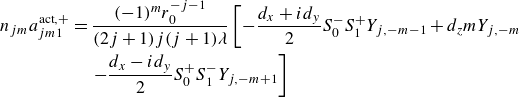 \begin{align} \begin{split} n_{jm}a_{jm1}^{{\mathrm {act}},+} &=\frac {(-1)^m r_0^{-j-1}}{(2j+1)j(j+1)\lambda }\left [ -\frac {d_x+i d_y}{2}S^-_0S^+_1Y_{j,-m-1}+d_z m Y_{j,-m}\right. \\ &\quad\left.-\frac {d_x -i d_y}{2}S^+_0S^-_1Y_{j,-m+1}\right ] \end{split} \end{align}
 \begin{align} \begin{split} &n_{jm}a_{jm2}^{{\mathrm {act}},+} = \frac {(-1)^m r_0^{-j-2} j}{(j+1)[(2j+1)(2j+3)]^{3/2}\lambda } \\ &\quad \left [-\frac {d_x+i d_y}{2}S^+_1S^+_2Y_{j+1,-m-1}-d_zS^+_1S^-_1Y_{j+1,-m}+\frac {d_x-i d_y}{2}S^-_1S^-_2Y_{j+1,-m+1} \right ]\end{split} \end{align}
 \begin{align} \begin{split} &n_{jm}a_{jm0}^{{\mathrm {act}},-} = \frac {(-1)^m r_0 ^{j-1}}{\lambda }\sqrt {\frac {2j+1}{2j-1}} \\ &\quad \left [-\frac {d_x+i d_y}{2} S^-_0S^-_{-1}Y_{j-1,-m-1}+ d_zS^+_0S^-_0Y_{j-1,-m}+\frac {d_x-i d_y}{2}S^+_0S^+_{-1}Y_{j-1,-m+1} \right ]\end{split} \end{align}
 \begin{align} \begin{split} n_{jm}a_{jm1}^{{\mathrm {act}},-} &=\frac {(-1)^m r_0^j}{\lambda } \left [-\frac {d_x+i d_y}{2} S^-_0S^+_1Y_{j,-m-1}+m d_z Y_{j,-m}\right. \\ &\quad \left.-\frac {d_x-i d_y}{2}S^+_0S^-_1Y_{j,-m+1} \right ]\end{split} \end{align}
 \begin{align} \begin{split} n_{jm}a_{jm2}^{{\mathrm {act}},-} &= \frac {(-1)^mr_0^{j+1}\sqrt {2j+1}}{2\lambda }\\ &\left [ \frac {(j+1)(2j+3)}{j} \left (- \frac {d_x+i d_y}{2} S^-_0S^-_{-1}Y_{j-1,-m-1}+d_zS^+_0S^-_0Y_{j-1,-m}\right. \right. \\ &\quad \left.+\frac {d_x-i d_y}{2}S^+_0S^+_1Y_{j-1,-m+1}\right ) \\ &\quad -\frac {2}{\sqrt {2j+3}}\left ( \frac {d_x+i d_y}{2}S^+_1S^+_2Y_{j+1,-m-1}+d_zS^+_1S^-_1Y_{j+1,-m}\right. \\ &\quad\left. \left.-\frac {d_x-i d_y}{2}Tp_1S^-_2Y_{j+1,-m+1}\right )\right ]. \end{split} \end{align}
B.4 Rotlet
The following are the coefficients for the expansion of the rotlet located at
 ${\boldsymbol {x}}_0 = (r_0,\theta _0,\phi _0)$
with axis of rotation
${\boldsymbol {x}}_0 = (r_0,\theta _0,\phi _0)$
with axis of rotation
 $(d_x,d_y,d_z)$
in a spherical coordinate system about the centre of the drop. The coefficients are in the
$(d_x,d_y,d_z)$
in a spherical coordinate system about the centre of the drop. The coefficients are in the
 ${\boldsymbol {u}}_{jm\sigma }^{FJ\pm }$
basis and can be converted to the basis used in this paper using (B5). As a shorthand we abbreviate
${\boldsymbol {u}}_{jm\sigma }^{FJ\pm }$
basis and can be converted to the basis used in this paper using (B5). As a shorthand we abbreviate
 $Y_{j,m} = y_{j,m}(\theta _0,\phi _0), S^+_k = \sqrt {j+m+k}, S^-_k = \sqrt {j-m+k}$
 \begin{align} &n_{jm}a_{jm0}^{{\mathrm {act}},+} = \frac {i(-1)^m r_0^{-j-1}}{2j(2j+1)\lambda }\left [ -\frac {d_x+i d_y}{2}S^-_0S^+_1Y_{j,-m-1}+m Y_{j,-m} \right. \nonumber \\ &\qquad\qquad\left. -\frac {d_x-i d_y}{2}S^+_0S^-_1Y_{j,-m+1}\right ] \nonumber \\ &n_{jm}a_{jm1}^{{\mathrm {act}},+} = \frac {i(-1)^m r_0^{-j-2}}{2(j+1)\lambda \sqrt {(2j+1)(2j+3)}} \nonumber \\ &\hspace {30pt}\left[-\frac {d_x+i d_y}{2}S^+_1S^+_2Y_{j+1,-m-1}-d_zS^+_1S^-_1Y_{j+1,-m}+\frac {d_x-i d_y}{2}S^-_1S^-_2Y_{j+1,-m+1} \right]&& \nonumber \\ &n_{jm}a_{jm2}^{{\mathrm {act}},+} = 0 \end{align}
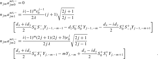 \begin{align} &n_{jm}a_{jm0}^{{\mathrm {act}},-} = 0 \nonumber \\ &n_{jm}a_{jm1}^{{\mathrm {act}},-} = \frac {i(-1)^m r_0^{j-1}}{2\lambda }(j+1) \sqrt {\frac {2j+1}{2j-1}} \nonumber \\ &\hspace {30pt}\left [\frac {d_x+i d_y}{2}S^-_0S^-_{-1}Y_{j-1,-m-1}-d_zS^-_0S^+_0Y_{j-1,-m}-\frac {d_x-i d_y}{2}S^+_0S^+_{-1}Y_{j-1,-m+1} \right ]&& \nonumber \\ &n_{jm}a_{jm2}^{{\mathrm {act}},-} = \frac {i (-1)^m (2j+1)(2j+3) r_0^j}{2j\lambda } \sqrt {\frac {2j+1}{2j-1}} \nonumber \\ &\hspace {30pt}\left [\frac {d_x+i d_y}{2}S^-_0S^-_1Y_{j,-m-1}-m Y_{j,-m} +\frac {d_x-i d_y}{2}S^+_0S^+_1Y_{j,-m+1}\right ]&& .\end{align}
B.5 Axisymmetric stresslet
The following are the coefficients for the expansion of the axisymmetric stresslet located at
 ${\boldsymbol {x}}_0 = (r_0,\theta _0,\phi _0)$
with orientation
${\boldsymbol {x}}_0 = (r_0,\theta _0,\phi _0)$
with orientation
 $(d_x,d_y,d_z)$
in a spherical coordinate system about the centre of the drop.. The coefficients are in the
$(d_x,d_y,d_z)$
in a spherical coordinate system about the centre of the drop.. The coefficients are in the
 ${\boldsymbol {u}}_{jm\sigma }^{FJ\pm }$
basis and can be converted to the basis used in this paper using (B5). As a shorthand we abbreviate
${\boldsymbol {u}}_{jm\sigma }^{FJ\pm }$
basis and can be converted to the basis used in this paper using (B5). As a shorthand we abbreviate
 $Y_{j,m} = y_{j,m}(\theta _0,\phi _0), S^+_k = \sqrt {j+m+k}, S^-_k = \sqrt {j-m+k}$
 \begin{align} \begin{split} n_{jm}a_{jm0}^{{\mathrm {act}},-} &= \frac {(-1)^m P r_0^{j-2}}{\lambda }\sqrt {\frac {2j+1}{2j-3}} \left [\frac {(d_x+i d_y)^2}{4}S^-_0S^-_{-1}S^-_{-2}S^-_{-3}Y_{j-2,-m-2}\right. \\ &\quad -(d_x+i d_y) d_z S^-_0S^-_{-1}S^-_{-2}S^+_0Y_{j-2,-m-1}-\frac {1-3d_z^2}{2}S^-_0S^-_{-1}S^+_0S^+_{-1}Y_{j-2,-m} \\ &\quad\left. +(d_x-i d_y) d_zS^-_0S^+_0S^+_{-1}S^+_{-2}Y_{j-2,-m+1}\right.\\ &\quad\left.+\frac {(d_x-i d_y)^2}{4}S^+_0S^+_{-1}S^+_{-2}S^+_{-3}Y_{j-2,-m+2}\right ]\end{split} \end{align}
 \begin{align} \begin{split} n_{jm}a_{jm1}^{{\mathrm {act}},-} &= \frac {(-1)^m P r_0^{j-1}}{2\lambda }\sqrt {\frac {2j+1}{2j-1}} \left [\frac {(d_x+i d_y)^2}{2}S^+_1S^-_0S^-_{-1}S^-_{-2}Y_{j-1,-m-2}\right. \\ &\quad-(d_x+i d_y)d_z (j+2m+1)S^-_0S^-_{-1}Y_{j-1,-m-1}-m(1-3d_z^2)S^+_0S^-_0Y_{j-1,-m} \\ &\quad\left. -(d_x-i d_y)d_z(j-2m+1)S^+_0S^+_{-1}Y_{j-1,-m-1}\right.\\ &\quad\left.-\frac {(d_x-id_y)^2}{2}S^-_1S^+_0S^+_{-1}S^+_{-2}Y_{j-1,-m+2} \right ]\end{split} \end{align}
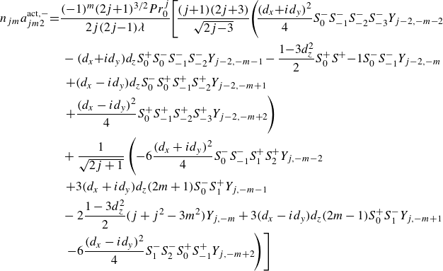 \begin{align} \begin{split} n_{jm}a_{jm2}^{{\mathrm {act}},-} & \!=\! \frac {(-1)^m (2j\!+\!1)^{3/2} P r_0^j}{2j(2j\!-\!1)\lambda }\!\left [\!\frac {(j\!+\!1)(2j\!+\!3)}{\sqrt {2j\!-\!3}}\!\left (\! \frac {(d_x\!+\!id_y)^2}{4}S^-_0S^-_{-1}S^-_{-2}S^-_{-3}Y_{j-2,-m-2}\right. \right. \\ &\quad -(d_x\!+\!id_y)d_zS^+_0S^-_0S^-_{-1}S^-_{-2}Y_{j-2,-m-1}-\frac {1\!-\!3d_z^2}{2}S^+_0S^+{-1}S^-_0S^-_{-1}Y_{j-2,-m} \\ &\quad\left. +(d_x-id_y)d_z S^-_0S^+_0S^+_{-1}S^+_{-2}Y_{j-2,-m+1}\right.\\ &\quad \left. +\frac {(d_x-id_y)^2}{4}S^+_0S^+_{-1}S^+_{-2}S^+_{-3}Y_{j-2,-m+2}\right ) \\ &\quad +\frac {1}{\sqrt {2j+1}}\left ( -6\frac {(d_x+id_y)^2}{4}S^-_0S^-_{-1}S^+_1S^+_2Y_{j,-m-2}\right.\\ &\quad \left. +3(d_x+id_y)d_z (2m+1)S^-_0S^+_1Y_{j,-m-1}\right. \\ &\quad -2\frac {1-3d_z^2}{2}(j+j^2-3m^2)Y_{j,-m}+3(d_x-id_y)d_z (2m-1)S^+_0S^-_1Y_{j,-m+1}\\ &\quad\left. \left. -6\frac {(d_x-id_y)^2}{4} S^-_1S^-_2S^+_0S^+_{-1}Y_{j,-m+2}\right )\right ]\end{split} \end{align}
 \begin{align} \begin{split} n_{jm}a_{jm0}^{{\mathrm {act}},+} &= \frac {(-1)^m P r_0^{-j-1}}{2(2j+3)\lambda }\left [\frac {1}{(2j+1)(2j-1)j}\left (\frac {3(d_x+id_y)^2}{2}S^-_0S^-_{-1}S^+_1S^+_2Y_{j,-m-2}\right. \right. \\ &\quad -3(d_x+id_y)d_z(2m+1)S^-_0S^+_1Y_{j,-m-1}+(1-3d_z^2)(j+j^2-3m^2)Y_{j,-m} \\ &\quad\left. +3(d_x-id_y)^2S^+_0S^-_1Y_{j,-m+1}+\frac {3(d_x-id_y)^2}{2}S^+_0S^+_{-1}S^-_1S^-_2Y_{j,-m+2}\right ) \\ &\quad+\frac {1}{\sqrt {(2j+1)(2j+5)}}\left ( -\frac {(d_x+id_y)^2}{4}S^+_1S^+_2S^+_3S^+_4Y_{j+2,-m-2}\right. \\ &\quad-(d_x+i d_y)d_zS^-_1S^+_1S^+_2S^+_3Y_{j+2,-m-1}+\frac {1-3d_z^2}{2}S^+_1S^+_2S^-_1S^-_2Y_{j+2,-m} \\ &\quad\left.+(d_x-id_y)S^+_1S^-_1S^-_2S^-_3Y_{j+2,-m+1}+\frac {d_x-id_y)^2}{4}S^-_1S^-_2S^-_3S^-_4Y_{j+2,-m+2}\right ]\end{split} \end{align}
 \begin{align} \begin{split} n_{jm}a_{jm1}^{{\mathrm {act}},+} &= \frac {(-1)^m P r_0^{-j-2}}{2 j (j+1)\sqrt {(2j+1)(2j+3)}\lambda }\left [\frac {(d_x+id_y)^2}{2}S^-_0S^+_1S^+_2S^+_3Y_{j+1,-m-2} \right. \\ &\quad +(d_x+id_y)d_z(j-2m)S^+_1S^+_2Y_{j+1,-m-1}+(1-3d_z^2)mS^+_1S^-_1Y_{j+1,-m} \\ &\quad\left. +(d_x-id_y)d_z (j+2m)S^-_1S^-_2Y_{j+1,-m+2}\right.\\ &\quad\left. - \frac {(d_x-id_y)^2}{2}S^+_0S^-_1S^-_2S^-_3Y_{j+1,-m+2}\right ]\end{split} \end{align}
 \begin{align} \begin{split} n_{jm}a_{jm2}^{{\mathrm {act}},+} &= \frac {(-1)^m Pj r_0^{-j-3}}{(j+1)(2j+1)^{3/2}(j+3)\sqrt {2j+5}\lambda }\left [\frac {(d_x+id_y)^2}{4}S^+_1S^+_2S^+_3S^+_4Y_{j+2,-m-2}\right. \\ &\quad+(d_x+id_y)d_zS^-_1S^+_1S^+_2S^+_3Y_{j+2.-m-1}-\frac {1-3d_z^2}{2}S^+_1S^+_2S^-_1S^-_2Y_{j+2,-m} \\ &\quad\left. -(d_x\!-\!id_y)^2 S^+_1S^-_1S^-_2S^-_3Y_{j+2,-m+1}\!+\!\frac {(d_x-id_y)^2}{2}S^-_1S^-_2S^-_3S^-_3Y_{j+2,-m+2}\right ]. \end{split} \end{align}
Appendix C. Drop Velocity
The flow about a spherical droplet translating in response to an internal Stokeslet in Sprenger et al. (Reference Sprenger, Shaik, Ardekani, Lisicki, Mathijssen, Guzmán-Lastra, Löwen, Menzel and Daddi-Moussa-Ider2020) is obtained, in the frame of reference of the drop, as a superposition of the solution for a Stokeslet in a pinned (held in place) droplet with velocity field decaying to zero at infinity and the solution for a pinned drop with velocity at infinity equal to the drop translational velocity,
 $-{\boldsymbol {U}}$
. The additional flow gives rise to stresses on the interface f and the stress balance on the drop surface for the composite problem is
$-{\boldsymbol {U}}$
. The additional flow gives rise to stresses on the interface f and the stress balance on the drop surface for the composite problem is
 \begin{equation} ({\textbf {T}}^{\mathrm {out}}-{\textbf {T}}^{\mathrm {ins}}) \cdot {{\boldsymbol {\hat {r}}}} = \frac {2\gamma }{R}{{\boldsymbol {\hat {r}}}} + {{\textbf {f}}} ,\end{equation}
where
 $\gamma$
is the constant surface tension, and
$\gamma$
is the constant surface tension, and
 $R$
is the drop radius. Integrating C1 over the surface of the drop leads to
$R$
is the drop radius. Integrating C1 over the surface of the drop leads to
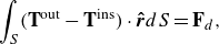 \begin{equation} \int _S ({\textbf {T}}^{\mathrm {out}}-{\textbf {T}}^{\mathrm {ins}}) \cdot {{\boldsymbol {\hat {r}}}} dS = {{\textbf{F}}}_{d} ,\end{equation}
where
 ${{\textbf{F}}}_{d}=\int {{\textbf {f}}} dS$
is the force on the droplet. Equation (32) in Sprenger et al. (Reference Sprenger, Shaik, Ardekani, Lisicki, Mathijssen, Guzmán-Lastra, Löwen, Menzel and Daddi-Moussa-Ider2020) is missing the contribution from the stress due to the interior flow. When considering flows applied externally to the drop such as Stokeslets outside the droplet as in Shaik & Ardekani (Reference Shaik and Ardekani2017) and Shaik et al. (Reference Shaik, Vasani and Ardekani2018), one has the Stokes equation
${{\textbf{F}}}_{d}=\int {{\textbf {f}}} dS$
is the force on the droplet. Equation (32) in Sprenger et al. (Reference Sprenger, Shaik, Ardekani, Lisicki, Mathijssen, Guzmán-Lastra, Löwen, Menzel and Daddi-Moussa-Ider2020) is missing the contribution from the stress due to the interior flow. When considering flows applied externally to the drop such as Stokeslets outside the droplet as in Shaik & Ardekani (Reference Shaik and Ardekani2017) and Shaik et al. (Reference Shaik, Vasani and Ardekani2018), one has the Stokes equation
 ${\boldsymbol {\nabla }} \cdot {\textbf {T}}^{\mathrm {ins}} = 0$
everywhere inside the droplet and thus it is sufficient to only consider the outside tractions
${\boldsymbol {\nabla }} \cdot {\textbf {T}}^{\mathrm {ins}} = 0$
everywhere inside the droplet and thus it is sufficient to only consider the outside tractions
 \begin{equation} \int _S {\textbf {T}}^{\mathrm {out}} \cdot {{\boldsymbol {\hat {r}}}} dS = {{\textbf{F}}}_{d}\,. \end{equation}
However, if a Stokeslet with strength
 ${{\textbf{F}}}_s$
is present inside the drop,
${{\textbf{F}}}_s$
is present inside the drop,
 ${\boldsymbol {\nabla }} \cdot {\textbf {T}}^{\mathrm {ins}} = -{{\textbf{F}}}_s\delta ({\boldsymbol {x}}-{\boldsymbol {x}}_0)$
and thus
${\boldsymbol {\nabla }} \cdot {\textbf {T}}^{\mathrm {ins}} = -{{\textbf{F}}}_s\delta ({\boldsymbol {x}}-{\boldsymbol {x}}_0)$
and thus
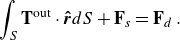 \begin{equation} \int _S {\textbf {T}}^{\mathrm {out}} \cdot {{\boldsymbol {\hat {r}}}} dS +{{\textbf{F}}}_s = {{\textbf{F}}}_{d}\,. \end{equation}
The velocity of the spherical clean drop is then
 \begin{equation} {\boldsymbol {U}}=\frac {(1+\lambda )}{2 \pi \mu R(2+3 \lambda )}\left (\int _S {\textbf {T}}^{\mathrm {out}} \cdot {{\boldsymbol {\hat {r}}}} dS +{{\textbf{F}}}_s\right ) .\end{equation}
Equation 5 for the drop velocity yields the same expression as ours, which is obtained from the volume averaged internal velocity, and the result reported by Kree et al. (Reference Kree, Rueckert and Zippelius2021). It differs from the result of Sprenger et al. (Reference Sprenger, Shaik, Ardekani, Lisicki, Mathijssen, Guzmán-Lastra, Löwen, Menzel and Daddi-Moussa-Ider2020) by the contribution of the internal Stokeslet to the net force on the drop. Our results for singularities other than the Stokeslet agree with those of Kree et al. (Reference Kree, Rueckert and Zippelius2021) and Sprenger et al. (Reference Sprenger, Shaik, Ardekani, Lisicki, Mathijssen, Guzmán-Lastra, Löwen, Menzel and Daddi-Moussa-Ider2020), since the internal tractions do not contribute to the force on the droplet.
Note that calculating the drop velocity as the volume-average of the internal velocity used in our paper is not limited to a spherical drop and can be used for a drop of any shape. The approach used in Sprenger et al. (Reference Sprenger, Shaik, Ardekani, Lisicki, Mathijssen, Guzmán-Lastra, Löwen, Menzel and Daddi-Moussa-Ider2020) requires knowledge of the mobility coefficient for the specific shape of the drop.


 Open access