


1. Introduction
1.1. Background
Lifted flames occur in some types of gas turbines, in many industrial furnaces and in several other important applications. Starting from an attached non-premixed jet flame, a lifted flame can be achieved by increasing the fuel-jet velocity such that an attached flame can no longer be supported. The flame then abruptly detaches and stabilises at some point downstream. The stabilisation location is a crucial parameter of a lifted flame. Longer lifted heights result from higher fuel injection velocities, and higher velocities are desirable to minimise the size of the fuel injection equipment and to increase the overall rate of mixing, allowing an overall smaller combustor. Longer lifted heights also lead to greater amounts of premixing before combustion, which – depending on the application – can lead to lower emissions of nitrogen oxides and/or soot. However, if the lifted height is too long, the flame can become unstable, which can be a problem because of thermo-acoustic dynamics as well as leading to increased emissions of unburned hydrocarbons and carbon monoxide. In extreme conditions, the flame can completely blow off, which is obviously undesirable in any combustion system.
Because of the importance of the lifted flames in combustion systems and the importance of the stabilisation dynamics to the overall combustion behaviour, the stabilisation mechanism has been extensively investigated. As nicely summarised in some key review articles (Pitts Reference Pitts1989; Lyons et al.
Reference Lyons, Watson, Carter and Donbar2007; Lawn Reference Lawn2009), several theories have been proposed. In the present study, we categorise and somewhat reinterpret these into four essential mechanisms which apply in an environment of oxidiser that has a temperature below the chain branching temperature such that autoignition can be ruled out. The mechanisms, which are sketched in figure 1, are categorised as the premixed flame theories, the edge-flame theories, the critical dissipation rate theories and the theories involving a role played by large eddies. The first attempt to shed light on the stabilisation mechanism was the study by Vanquickenborne & van Tiggelen (Reference Vanquickenborne and van Tiggelen1966), which proposed that the flame base is the location where the jet average velocity is equal to the turbulent premixed flame speed. Later, Kalghatgi (Reference Kalghatgi1984) proposed an adjustment to this concept in which the turbulent premixed flame speed is related to the turbulence intensity. It has been shown since then that in cases when the lift-off height is 20 times greater than the jet diameter
 $D$
, this theory has significant support (Lawn Reference Lawn2009). Here, to distinguish this theory from the edge-flame theory, introduced below, we slightly clarify the concept to state that it involves a broad flammable region with width significantly larger than the laminar flame thickness.
$D$
, this theory has significant support (Lawn Reference Lawn2009). Here, to distinguish this theory from the edge-flame theory, introduced below, we slightly clarify the concept to state that it involves a broad flammable region with width significantly larger than the laminar flame thickness.

Figure 1. Schematic of a lifted jet flame (centre), and different theories for the stabilisation. Specific references for these theories are discussed below.
The edge-flame stabilisation mechanism, which was originally proposed by Buckmaster & Weber (Reference Buckmaster and Weber1996), is based on the concept that a partially premixed edge flame supports the flame by upstream propagation along the stoichiometric surface. There have been a large number of theoretical, experimental and numerical studies of laminar edge flames (Peters & Kee Reference Peters and Kee1987; Ruetsch, Vervisch & Liñán Reference Ruetsch, Vervisch and Liñán1995; Buckmaster Reference Buckmaster1996; Vedarajan & Buckmaster Reference Vedarajan and Buckmaster1998; Ghosal & Vervisch Reference Ghosal and Vervisch2000; Buckmaster Reference Buckmaster2002; Boulanger et al. Reference Boulanger, Vervisch, Reveillon and Ghosal2003; Chung Reference Chung2007), which show that edge flames can be stabilised in laminar jets by propagation relative to the flow. Moreover, their propagation speed can significantly exceed the burning velocity of a flat flame due to streamline divergence around the flame (Ruetsch et al. Reference Ruetsch, Vervisch and Liñán1995).
Considerable evidence for the existence of edge-flame structures has been accumulated in experimental studies of turbulent lifted flames (for example Stårner et al. Reference Stårner, Bilger, Frank, Marran and Long1996; Muniz & Mungal Reference Muniz and Mungal1997; Hasselbrink & Mungal Reference Hasselbrink and Mungal1998; Watson et al. Reference Watson, Lyons, Donbar and Carter2000, Reference Watson, Lyons, Donbar and Carter2003; Arndt et al. Reference Arndt, Schießl, Gounder, Meier and Aigner2013). In our interpretation of this theory, as distinct from the premixed flame theory, a much narrower flammable region exists with width significantly smaller than the turbulence integral scale and up to several laminar flame thicknesses. Depending on the conditions, edge flames may have distinct rich and/or lean branches, but when the flammable region is narrow, the lean and rich branches are collapsed into a single-branched structure.
Peters & Williams (Reference Peters and Williams1983) proposed the critical scalar dissipation theory, where the flame is stabilised because it cannot move further upstream due to the local scalar dissipation rates (i.e. gradients) being too high. Initially, it was proposed that the critical scalar dissipation rate should correspond to the extinction dissipation rate of a diffusion flame (Peters & Williams Reference Peters and Williams1983). Later, it was judged that scalar dissipation rates at the flame base were insufficient to support such a mechanism (Müller, Breitbach & Peters Reference Müller, Breitbach and Peters1994). There have been experimental studies supporting (Namazian, Schefer & Kelly Reference Namazian, Schefer and Kelly1988) or opposing (Schefer, Namazian & Kelly Reference Schefer, Namazian and Kelly1994b ; Hasselbrink & Mungal Reference Hasselbrink and Mungal1998; Watson et al. Reference Watson, Lyons, Donbar and Carter2003) this theory. However, the literature suggests that, so far, the role of the scalar dissipation rate in the stabilisation of the flame cannot be completely ruled out (Lawn Reference Lawn2009).
Here, we somewhat reinterpret the critical scalar dissipation concept and restate the hypothesis that the critical scalar dissipation rate can also be that at which the local edge-flame velocity becomes significantly lower than the unstrained burning velocity, such that it cannot match the flow velocity and hence moves further downstream. This can occur at a substantially lower scalar dissipation rate than the extinction scalar dissipation rate of an established diffusion flame.
There has been significant interest in the role of large eddies in flame stabilisation. Broadwell, Dahm & Mungal (Reference Broadwell, Dahm and Mungal1985) originally proposed that large structures cause hot reaction products to be ejected to the edges of the jet and then re-enter the jet together with fresh oxidiser and reinitiate combustion. As discussed by Broadwell et al. (Reference Broadwell, Dahm and Mungal1985), this mechanism does not completely explain the phenomena surrounding stabilisation since it cannot explain the upstream motion of a lifted flame that is ignited downstream of its lifted stabilisation point. To explain this aspect, upstream transport is certainly required, but this is typically not observed experimentally.
Several other works have suggested stabilisation mechanisms that involve a strong influence of large eddies. First, it should be mentioned that all theories based on turbulent premixed flame propagation naturally involve the effect of eddies to increase the burning velocity. What distinguishes the theories discussed below is that they involve coherent eddies associated with large-scale jet organisation, while the turbulent premixed flame concept does not explicitly take this organisation into account.
Miake-Lye & Hammer (Reference Miake-Lye and Hammer1989) proposed a mechanism that is related to the critical dissipation rate concept wherein the flame is stabilised in a region where the large-scale strain rate is lower than a critical level (as opposed to the original scalar dissipation concept based on a small-scale strain rate). It was proposed that the flame propagates from one structure to its upstream neighbour until the strain rate between the structures exceeds a critical value, and the flame moves downstream again. The lifted height and the inlet jet velocity were shown to have a linear correlation, and this behaviour was suggested to be consistent with the proposed concept based on a self-similar form of the large-scale strain rate field which decays inversely proportional to axial distance.
Burgess & Lawn (Reference Burgess and Lawn1999) proposed another hybrid concept wherein a turbulent premixed flame is involved, but large eddies play a moderating role through outer-scale intermittency. Once intermittency was accounted for, turbulent burning velocity correlations from Abdel-Gayed, Bradley & Lawes (Reference Abdel-Gayed, Bradley and Lawes1987) were found to agree within a factor of two with the estimated turbulent burning velocity in the intermittent large eddies of turbulent fluid.
We refer to figure 2, taken from Su, Sun & Mungal (Reference Su, Sun and Mungal2006) (permission has been obtained from the authors), to explain this idea. Since the concept is nicely stated in that article, we simply quote the explanation, and the figure’s caption.
In (a), the stabilisation point is relatively far from the centreline, and the flame advances upstream against the low axial flow velocity. This simultaneously requires that the flame move radially inward, to maintain a flammable mixture. Eventually, the local axial flow velocity becomes sufficiently high that the flame begins to recede downstream (b). When the trailing coherent structure, which brings higher fuel mole fractions, overtakes the flame, the stabilisation point moves radially outward (c). As the flame moves downstream and outward, the flow axial velocity decreases, until the flame once again propagates upstream (d) and the initial situation recurs (e).

Figure 2. ‘Schematic depiction of the flame-base motion, in terms of the axisymmetric mode of large-scale organisation of the mixing field. Time advances from left to right. The instantaneous stabilisation point for each time is represented by a grey circle.’ Caption and figure from Su et al. (Reference Su, Sun and Mungal2006), with permission from the authors.
A different theory involving both flame propagation and large-eddy structures in the stabilisation was proposed by Lawn (Reference Lawn2009). In this scenario, a large structure of rich mixture departs from the fuel jet upstream of the flame and is diluted as it moves towards the oxidiser stream. This flammable mixture will move downstream and eventually encounter the hot region and ignite. The ignited mixture then propagates in the shape of an edge flame or triple flame downstream within the eddy leaving the hot products behind for the next eddy to come.
Some other studies support the coexistence of different theories (Kaplan, Oran & Baek Reference Kaplan, Oran and Baek1994; Schefer et al. Reference Schefer, Namazian and Kelly1994b ).
Other structures that may play a role in the stabilisation, which have been reported in recent experimental studies, are isolated flame islands in two-dimensional (2D) laser-based measurements which do not appear to be connected to the main flame. Lyons et al. (Reference Lyons, Watson, Carter and Donbar2007) reported the presence of these islands and proposed that they might be introduced by out-of-plane motions. Similar structures were observed in a series of experimental studies by Boxx et al. (Reference Boxx, Heeger, Gordon, Böhm, Aigner, Dreizler and Meier2009a ,Reference Boxx, Heeger, Gordon, Böhm, Dreizler and Meier b ). Gordon et al. (Reference Gordon, Boxx, Carter, Dreizler and Meier2012) reported a significant out-of-plane velocity prior to the appearance of the flame islands, confirming that out-of-plane motion plays a role. They did not observe any correlation between flame motion and turbulent intensity and large structures, neither was there a significant flow field divergence upstream of the flame base. Hence, they proposed that out-of-plane motion was the main reason for stabilisation.
As outlined briefly above and more comprehensively in the review articles by Pitts (Reference Pitts1989), Lyons et al. (Reference Lyons, Watson, Carter and Donbar2007) and Lawn (Reference Lawn2009), the stabilisation mechanism has still not been determined. It has been widely reported that flame propagation plays a key role; however, to the best of our knowledge there has been no complete experimental measurement of edge-flame velocities, principally because the out-of-plane flame propagation is unknown. A few experimental studies have reported relative flame propagation velocities (Hasselbrink & Mungal Reference Hasselbrink and Mungal1998; Watson et al. Reference Watson, Lyons, Carter and Donbar2002; Upatnieks et al. Reference Upatnieks, Driscoll, Rasmussen and Ceccio2004; Heeger et al. Reference Heeger, Böhm, Ahmed, Gordon, Boxx, Meier, Dreizler and Mastorakos2009; Gordon et al. Reference Gordon, Boxx, Carter, Dreizler and Meier2012). In all of these studies, the flow velocity is measured using particle image velocimetry (PIV). The absolute edge-flame velocity is accessible by comparing flame-base location in two sequential measurements of the flame base. To mark the flame location, some experiments used the evaporation of liquid PIV seeding particles (Hasselbrink & Mungal Reference Hasselbrink and Mungal1998), which involved a large uncertainty, while others used planar laser-induced fluorescence (PLIF) of a radical species, such as OH or CH (Watson et al. Reference Watson, Lyons, Carter and Donbar2002; Upatnieks et al. Reference Upatnieks, Driscoll, Rasmussen and Ceccio2004; Heeger et al. Reference Heeger, Böhm, Ahmed, Gordon, Boxx, Meier, Dreizler and Mastorakos2009; Gordon et al. Reference Gordon, Boxx, Carter, Dreizler and Meier2012). While uncertainties associated with measuring the flame location are reduced by applying the latter method, there are other systematic errors that should be considered. The main challenge is a lack of knowledge of the out-of-plane velocities or any knowledge of flame structure in the third dimension. To partly address this challenge, Gordon et al. (Reference Gordon, Boxx, Carter, Dreizler and Meier2012) conditioned their results on low out-of-plane velocities, but this still does not capture out-of-plane flame propagation. This is the principal gap that the present article addresses. The presented direct numerical simulation (DNS) data provide both the flow and propagation velocities in three dimensions, which eliminates the uncertainties embedded in the above experimental studies.
It is also worth recounting the main results of previous relevant DNS studies of lifted turbulent flames. Only very few previous such studies have appeared. In a very early and informative study, Mizobuchi et al. (Reference Mizobuchi, Tachibana, Shinio, Ogawa and Takeno2002, Reference Mizobuchi, Shinio, Ogawa and Takeno2005) considered a lifted hydrogen flame. The flame exhibited a vigorous rich inner premixed flame surrounded by a region of lean mixtures having generally low reaction rates except in isolated islands of diffusion flames. It is important to note here that hydrogen is a fuel that has totally different characteristics from hydrocarbon fuel. Hydrogen can sustain a premixed flame at significantly richer and leaner mixtures than a hydrocarbon can. This fundamental difference could have significant consequences for the stabilisation mechanism.
Yoo, Sankaran & Chen (Reference Yoo, Sankaran and Chen2009) considered DNS of a lifted hydrogen flame in a hot coflow, while Yoo et al. (Reference Yoo, Richardson, Sankaran and Chen2011) considered an ethylene jet flame in a highly heated coflow. In both cases, the flames were found to be stabilised by autoignition, with moderating roles played by the scalar dissipation rate and a similar mechanism involving large eddies as reported by Su et al. (Reference Su, Sun and Mungal2006) being noted. It is, however, obvious that a flame in a cold oxidiser environment can have a different stabilisation mechanism compared with these studies.
1.2. Objectives
The particular objectives of this DNS-based study are as follows. The first objective is to qualitatively report the instantaneous structure of a lifted flame that is representative of a hydrocarbon, describing interesting features of the edge flames, and comparing the observations against previous experimental work and against theoretical concepts to explain lifted flame stabilisation. The second objective is to quantify the motion of the flame base in an instantaneous and local manner, in order to reveal the roles played by flame propagation and turbulent eddies, and thus propose the flame stabilisation mechanism. The final objective is to analyse the flame base from an averaged standpoint to provide additional support for the proposed mechanism.
Given these objectives, it was considered important to simulate a case having key parameters that overlapped with experimentally measured lifted flames. In particular, it was considered important to approximately match the ratio of the jet velocity to the laminar flame speed (
 $\boldsymbol{U}_{j}/S_{L}$
), the ratio of the jet width to the laminar flame thickness (
$\boldsymbol{U}_{j}/S_{L}$
), the ratio of the jet width to the laminar flame thickness (
 $H/{\it\delta}_{L}$
), the Reynolds number (Re) and the ratio of burned to unburned densities (
$H/{\it\delta}_{L}$
), the Reynolds number (Re) and the ratio of burned to unburned densities (
 ${\it\rho}_{b}/{\it\rho}_{u}$
). The use of practically relevant values of
${\it\rho}_{b}/{\it\rho}_{u}$
). The use of practically relevant values of
 $H/{\it\delta}_{L}$
and Re imposed stringent computational demands. In addition, a large domain and long integration time were required to achieve sufficient realism and statistics. Finally, although we only report results from one case in this article, our wider objectives include understanding how the stabilisation mechanism depends on key parameters; this requires a series of parameter runs.
$H/{\it\delta}_{L}$
and Re imposed stringent computational demands. In addition, a large domain and long integration time were required to achieve sufficient realism and statistics. Finally, although we only report results from one case in this article, our wider objectives include understanding how the stabilisation mechanism depends on key parameters; this requires a series of parameter runs.
Yoo et al. (Reference Yoo, Sankaran and Chen2009, Reference Yoo, Richardson, Sankaran and Chen2011) employed detailed chemical kinetic models; however, the computational cost of these models is extreme, in the range of tens of millions of computer core hours per run, which is not feasible at present except for very few groups. It was clear that detailed chemistry would not be feasible given the present objectives and available computing time. In this work, it was therefore necessary to simplify the thermochemistry. In order to achieve the maximum realism of the above listed parameters, it was decided to use the very simplest thermochemical model that could represent hydrocarbon combustion, i.e. a one-step chemistry model. The one-step mechanism employed an empirical adjustment to reproduce the decreasing dependence of the hydrocarbon flame speed on the equivalence ratio in rich mixtures, as suggested by Garrido-Lòpez & Sarkar (Reference Garrido-Lòpez and Sarkar2005). Further justification for this choice, including cost estimates for a run with a four-step chemistry model and the same parameter settings as the present run, is discussed later.
2. Methods
2.1. Governing equations
The conservation equations of mass, momentum, sensible energy and mass fraction of fuel (
 $F$
) and oxidiser (
$F$
) and oxidiser (
 $O$
) are solved considering a one-step irreversible reaction of
$O$
) are solved considering a one-step irreversible reaction of
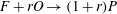 $F+rO\rightarrow (1+r)P$
, where
$F+rO\rightarrow (1+r)P$
, where
 $r$
is the stoichiometric ratio. These equations are non-dimensionalised as follows, where the superscript ‘*’ represents dimensional values and the subscript ‘
$r$
is the stoichiometric ratio. These equations are non-dimensionalised as follows, where the superscript ‘*’ represents dimensional values and the subscript ‘
 $o$
’ is the fuel stream conditions at the inlet:
$o$
’ is the fuel stream conditions at the inlet:
 $$\begin{eqnarray}\left.\begin{array}{@{}cccccc@{}}\boldsymbol{x}_{j}=\displaystyle \frac{\boldsymbol{x}_{j}^{\ast }}{H}, & \displaystyle \boldsymbol{U}_{j}=\frac{\boldsymbol{U}_{j}^{\ast }}{a_{o}^{\ast }}, & \displaystyle {\it\rho}=\frac{{\it\rho}^{\ast }}{{\it\rho}_{o}^{\ast }}, & \displaystyle t=\frac{t^{\ast }a_{o}^{\ast }}{H}, & \displaystyle p=\frac{p^{\ast }}{{\it\rho}_{o}^{\ast }a_{o}^{\ast 2}}, & \displaystyle T=\frac{T^{\ast }}{({\it\gamma}-1)T_{o}^{\ast }},\\ \displaystyle {\it\mu}=\frac{{\it\mu}^{\ast }}{\mathit{Re}{\it\mu}_{o}^{\ast }}, & \displaystyle \mathit{Pr}=\frac{{\it\upsilon}^{\ast }}{{\it\alpha}^{\ast }}, & \displaystyle \mathit{Le}=\frac{{\it\alpha}^{\ast }}{D^{\ast }}, & \displaystyle \mathit{Re}=\frac{{\it\rho}_{o}^{\ast }a_{o}^{\ast }H}{{\it\mu}_{o}^{\ast }}, & \displaystyle \mathit{Da}=A\frac{H{\it\rho}_{o}^{\ast }}{a_{o}^{\ast }}, & \mathit{Sc}=\mathit{Le}\mathit{Pr}.\end{array}\right\}\end{eqnarray}$$
In the above,
 $\boldsymbol{x}_{j}$
represents the spatial vector,
$\boldsymbol{x}_{j}$
represents the spatial vector,
 $H$
the inlet jet width,
$H$
the inlet jet width,
 $\boldsymbol{U}_{j}$
the velocity vector,
$\boldsymbol{U}_{j}$
the velocity vector,
 $a$
the speed of sound,
$a$
the speed of sound,
 ${\it\rho}$
the density,
${\it\rho}$
the density,
 $T$
the temperature,
$T$
the temperature,
 $t$
time,
$t$
time,
 $p$
the pressure,
$p$
the pressure,
 ${\it\gamma}$
the heat capacity ratio and
${\it\gamma}$
the heat capacity ratio and
 ${\it\mu}$
the dynamic viscosity, which is given by
${\it\mu}$
the dynamic viscosity, which is given by
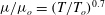 ${\it\mu}/{\it\mu}_{o}=(T/T_{o})^{0.7}$
. The variable Re represents the Reynolds number, Le the Lewis number, Pr the Prandtl number, Sc the Schmidt number and
${\it\mu}/{\it\mu}_{o}=(T/T_{o})^{0.7}$
. The variable Re represents the Reynolds number, Le the Lewis number, Pr the Prandtl number, Sc the Schmidt number and
 $A$
the pre-exponential factor in the Arrhenius law. Therefore, the non-dimensional inlet temperature is 2.5 considering
$A$
the pre-exponential factor in the Arrhenius law. Therefore, the non-dimensional inlet temperature is 2.5 considering
 ${\it\gamma}=1.4$
. The non-dimensional forms of the equations are:
${\it\gamma}=1.4$
. The non-dimensional forms of the equations are:
 $$\begin{eqnarray}\left.\begin{array}{@{}c@{}}\displaystyle \frac{\partial {\it\rho}}{\partial t}+\frac{\partial {\it\rho}\boldsymbol{U}_{i}}{\partial \boldsymbol{x}_{i}}=0,\\ \displaystyle \frac{\partial {\it\rho}\boldsymbol{U}_{i}}{\partial t}+\frac{\partial {\it\rho}\boldsymbol{U}_{i}\boldsymbol{U}_{j}}{\partial \boldsymbol{x}_{j}}=-\frac{\partial p}{\partial \boldsymbol{x}_{i}}+\frac{\partial {\it\tau}_{ij}}{\partial \boldsymbol{x}_{j}},\\ \displaystyle \frac{\partial {\it\rho}E}{\partial t}+\frac{\partial \boldsymbol{U}_{j}({\it\rho}E+p)}{\partial \boldsymbol{x}_{j}}=\frac{\partial \boldsymbol{U}_{i}{\it\tau}_{ij}}{\partial \boldsymbol{x}_{j}}-\frac{\partial \boldsymbol{q}_{j}}{\partial \boldsymbol{x}_{j}}-\frac{{\it\tau}\dot{{\it\omega}}_{F}}{Y_{Fst}({\it\gamma}-1)}\\ \displaystyle \text{and}\quad \frac{\partial {\it\rho}Y_{k}}{\partial t}+\frac{\partial {\it\rho}\boldsymbol{U}_{j}Y_{k}}{\partial \boldsymbol{x}_{j}}=\frac{\partial }{\partial \boldsymbol{x}_{j}}\left(\frac{1}{\mathit{Sc}}{\it\mu}\frac{\partial Y_{k}}{\partial \boldsymbol{x}_{j}}\right)+\dot{{\it\omega}}_{k},\quad k=F,O,\end{array}\right\}\end{eqnarray}$$
where
 $$\begin{eqnarray}\left.\begin{array}{@{}c@{}}\displaystyle p=\frac{{\it\gamma}-1}{{\it\gamma}}{\it\rho}T,\\ \displaystyle {\it\tau}_{ij}={\it\mu}\left[\frac{\partial \boldsymbol{U}_{i}}{\partial \boldsymbol{x}_{j}}+\frac{\partial \boldsymbol{U}_{j}}{\partial \boldsymbol{x}_{i}}-\frac{2}{3}\frac{\partial \boldsymbol{U}_{k}}{\partial \boldsymbol{x}_{k}}{\it\delta}_{ij}\right],\\ \displaystyle \boldsymbol{q}_{j}=-\frac{{\it\mu}}{\mathit{Pr}}\frac{\partial T}{\partial \boldsymbol{x}_{j}},\\ \displaystyle \dot{{\it\omega}}_{F}=\frac{1}{r}\dot{{\it\omega}}_{O}=-\mathit{Da}{\it\rho}^{2}Y_{F}Y_{O}\exp \left[-\frac{{\it\beta}(1-T^{\prime })}{1-{\it\alpha}(1-T^{\prime })}\right],\\ \displaystyle T^{\prime }=\frac{({\it\gamma}-1)T-1}{{\it\tau}},\\ \displaystyle E=\frac{T}{{\it\gamma}}+\frac{1}{2}\boldsymbol{U}_{k}\boldsymbol{U}_{k},\\ \displaystyle {\it\tau}={\it\alpha}/(1-{\it\alpha}),\\ {\it\alpha}=\displaystyle \frac{({\it\gamma}-1)T_{ad}-1}{({\it\gamma}-1)T_{ad}}\quad \text{and}\\ \displaystyle Y_{Fst}=\frac{Y_{F,o}}{1+rY_{F,o}/Y_{O,o}}.\end{array}\right\}\end{eqnarray}$$
Here,
 ${\it\tau}_{ij}$
is the shear stress tensor,
${\it\tau}_{ij}$
is the shear stress tensor,
 $\boldsymbol{q}_{i}$
is the heat flux vector,
$\boldsymbol{q}_{i}$
is the heat flux vector,
 $\dot{{\it\omega}}_{F}$
is the fuel reaction rate,
$\dot{{\it\omega}}_{F}$
is the fuel reaction rate,
 $Y$
is the mass fraction,
$Y$
is the mass fraction,
 $E$
is the sensible internal energy,
$E$
is the sensible internal energy,
 $T_{ad}$
is the adiabatic flame temperature and the subscripts
$T_{ad}$
is the adiabatic flame temperature and the subscripts
 $F$
and
$F$
and
 $O$
correspond to fuel and oxidiser respectively.
$O$
correspond to fuel and oxidiser respectively.
The Zel’dovich number (
 ${\it\beta}$
), i.e. normalised activation energy, which appears in (2.3) was modified as suggested by Garrido-Lòpez & Sarkar (Reference Garrido-Lòpez and Sarkar2005) to capture the experimentally observed dependence of the laminar burning rate
${\it\beta}$
), i.e. normalised activation energy, which appears in (2.3) was modified as suggested by Garrido-Lòpez & Sarkar (Reference Garrido-Lòpez and Sarkar2005) to capture the experimentally observed dependence of the laminar burning rate
 $S_{L}$
on the equivalence ratio, in particular the significant reduction of
$S_{L}$
on the equivalence ratio, in particular the significant reduction of
 $S_{L}$
in very rich mixtures. Therefore, the Zel’dovich number is defined as
$S_{L}$
in very rich mixtures. Therefore, the Zel’dovich number is defined as
 $$\begin{eqnarray}{\it\beta}({\it\phi})=\left\{\begin{array}{@{}lrl@{}}{\it\beta}_{0}[1+8.25({\it\phi}-0.64)^{2}], & & {\it\phi}\leqslant 0.64,\\ {\it\beta}_{0}, & 0.65<\, & {\it\phi}<1.07,\\ {\it\beta}_{0}[1+1.443({\it\phi}-1.07)^{2}], & & {\it\phi}\geqslant 1.07,\end{array}\right.\end{eqnarray}$$
where
 ${\it\beta}_{0}$
is 5.0 and
${\it\beta}_{0}$
is 5.0 and
 ${\it\phi}$
is the local equivalence ratio.
${\it\phi}$
is the local equivalence ratio.
2.2. Configuration
The configuration is a slot-jet flame similar to that studied in the previous DNS of lifted flames in hot oxidiser environments performed by Yoo et al. (Reference Yoo, Sankaran and Chen2009, Reference Yoo, Richardson, Sankaran and Chen2011) and is presented schematically in figure 3. The simulation parameters along with their values are presented in table 1. The mean inlet axial velocity
 $\boldsymbol{U}_{in}$
and fuel mass fraction
$\boldsymbol{U}_{in}$
and fuel mass fraction
 $Y_{F}$
were specified using a
$Y_{F}$
were specified using a
 $\tanh$
-based profile shown in figure 4 and given by
$\tanh$
-based profile shown in figure 4 and given by
 $$\begin{eqnarray}\boldsymbol{U}_{in}=\boldsymbol{U}_{c}+\frac{\boldsymbol{U}_{j}-\boldsymbol{U}_{c}}{2}\left(\tanh \left(\frac{y+H/2}{2{\it\delta}_{in}}\right)-\tanh \left(\frac{y-H/2}{2{\it\delta}_{in}}\right)\right),\end{eqnarray}$$
where
 $\boldsymbol{U}_{c}$
and
$\boldsymbol{U}_{c}$
and
 $\boldsymbol{U}_{j}$
are the mean coflow and mean inlet jet velocities, and the inlet momentum (and mixing layer) thickness,
$\boldsymbol{U}_{j}$
are the mean coflow and mean inlet jet velocities, and the inlet momentum (and mixing layer) thickness,
 ${\it\delta}_{in}$
, is equal to
${\it\delta}_{in}$
, is equal to
 $0.05H$
. Corresponding profiles were used for the fuel and oxidiser mass fractions. To describe the velocity fluctuations at the inlet,
$0.05H$
. Corresponding profiles were used for the fuel and oxidiser mass fractions. To describe the velocity fluctuations at the inlet,
 $u$
, a homogeneous isotropic turbulence field based on a prescribed turbulent energy spectrum (Passot & Pouquet Reference Passot and Pouquet1987) with a turbulence intensity of 5 % is first produced. These velocity fluctuations are then added to the mean inlet velocity and fed into the domain using Taylor’s hypothesis (Yoo et al.
Reference Yoo, Sankaran and Chen2009, Reference Yoo, Richardson, Sankaran and Chen2011). (The 5 % turbulent intensity in the inlet was selected based on experimental studies of Joedicke, Peters & Mansour (Reference Joedicke, Peters and Mansour2005). A top-hat profile for the bulk velocity was selected mainly for simplicity and consistency with previous DNS (Yoo et al.
Reference Yoo, Sankaran and Chen2009, Reference Yoo, Richardson, Sankaran and Chen2011). The authors acknowledge that some details of lifted flames have been shown to be dependent on burner geometry and boundary conditions, e.g. Akbarzadeh & Birouk (Reference Akbarzadeh and Birouk2014), but believe that the main phenomenology of the lifted flame stabilisation will remain the same for reasonable choices of boundary conditions.)
$u$
, a homogeneous isotropic turbulence field based on a prescribed turbulent energy spectrum (Passot & Pouquet Reference Passot and Pouquet1987) with a turbulence intensity of 5 % is first produced. These velocity fluctuations are then added to the mean inlet velocity and fed into the domain using Taylor’s hypothesis (Yoo et al.
Reference Yoo, Sankaran and Chen2009, Reference Yoo, Richardson, Sankaran and Chen2011). (The 5 % turbulent intensity in the inlet was selected based on experimental studies of Joedicke, Peters & Mansour (Reference Joedicke, Peters and Mansour2005). A top-hat profile for the bulk velocity was selected mainly for simplicity and consistency with previous DNS (Yoo et al.
Reference Yoo, Sankaran and Chen2009, Reference Yoo, Richardson, Sankaran and Chen2011). The authors acknowledge that some details of lifted flames have been shown to be dependent on burner geometry and boundary conditions, e.g. Akbarzadeh & Birouk (Reference Akbarzadeh and Birouk2014), but believe that the main phenomenology of the lifted flame stabilisation will remain the same for reasonable choices of boundary conditions.)

Figure 3. Schematic of the domain and the configuration of this study.

Figure 4. Mean profiles of the axial velocity, fuel and oxidiser mass fractions at the inlet.
Table 1. Numerical and physical parameters of the simulation.

Non-reflecting outflow boundary conditions were employed in the streamwise and transverse directions, and periodic boundary conditions were applied in the spanwise direction.
To determine appropriate simulation parameters, the bulk parameters were approximately matched with a case reported in Cessou, Maurey & Stepowski (Reference Cessou, Maurey and Stepowski2004). Therein,
 $S_{L}/\boldsymbol{U}_{j}=0.013$
,
$S_{L}/\boldsymbol{U}_{j}=0.013$
,
 ${\it\delta}_{L}/H=0.13$
and
${\it\delta}_{L}/H=0.13$
and
 $\mathit{Re}=5280$
while in our simulation we have
$\mathit{Re}=5280$
while in our simulation we have
 $S_{L}/\boldsymbol{U}_{j}=0.016$
,
$S_{L}/\boldsymbol{U}_{j}=0.016$
,
 ${\it\delta}_{L}/H=0.16$
and
${\it\delta}_{L}/H=0.16$
and
 $\mathit{Re}=5280$
; i.e. the bulk jet Reynolds number,
$\mathit{Re}=5280$
; i.e. the bulk jet Reynolds number,
 ${\it\rho}\boldsymbol{U}_{j}H/{\it\mu}$
, and the bulk jet Damköhler number,
${\it\rho}\boldsymbol{U}_{j}H/{\it\mu}$
, and the bulk jet Damköhler number,
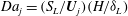 $\mathit{Da}_{j}=(S_{L}/\boldsymbol{U}_{j})(H/{\it\delta}_{L})$
, were exactly matched. It should be noted, however, that the experimental work considered a round jet while the DNS considered a slot jet, as it is a computationally much more affordable geometry. A round jet requires a larger domain to accommodate jet spreading in two directions, but more importantly it requires a much longer simulation time to achieve the same level of statistical convergence, particularly near the centreline.
$\mathit{Da}_{j}=(S_{L}/\boldsymbol{U}_{j})(H/{\it\delta}_{L})$
, were exactly matched. It should be noted, however, that the experimental work considered a round jet while the DNS considered a slot jet, as it is a computationally much more affordable geometry. A round jet requires a larger domain to accommodate jet spreading in two directions, but more importantly it requires a much longer simulation time to achieve the same level of statistical convergence, particularly near the centreline.
2.3. Numerical methods
The DNS code S3D_SC is employed here; S3D_SC is a modified version of the detailed chemistry code S3D (Chen et al. Reference Chen, Choudhary, De Supinski, Devries, Hawkes, Klasky, Liao, Ma, Mellor-Crummey, Podhorszki, Sankaran, Shende and Yoo2009) which solves equations described in § 2.1. The original DNS code S3D has been used in a large number of studies of combustion (for example Echekki & Chen Reference Echekki and Chen1998; Im & Chen Reference Im and Chen1999; Chen et al. Reference Chen, Choudhary, De Supinski, Devries, Hawkes, Klasky, Liao, Ma, Mellor-Crummey, Podhorszki, Sankaran, Shende and Yoo2009; Hawkes et al. Reference Hawkes, Sankaran, Chen, Kaiser and Frank2009; Yoo et al. Reference Yoo, Sankaran and Chen2009, Reference Yoo, Richardson, Sankaran and Chen2011; Grout et al. Reference Grout, Gruber, Kolla, Bremer, Bennett, Gyulassy and Chen2012; Hawkes et al. Reference Hawkes, Chatakonda, Kolla, Kerstein and Chen2012; Kolla et al. Reference Kolla, Grout, Gruber and Chen2012; Luo et al. Reference Luo, Yoo, Richardson, Chen, Law and Lu2012; Chatakonda et al. Reference Chatakonda, Hawkes, Aspden, Kerstein, Kolla and Chen2013; Krisman et al. Reference Krisman, Hawkes, Talei, Bhagatwala and Chen2015). Like S3D, the solver S3D_SC uses high-order accurate, low-dissipation numerical schemes and a 3D structured Cartesian mesh. Spatial derivatives were computed using an eighth-order central differencing scheme and time integration was performed with a six-stage fourth-order explicit Runge–Kutta method. To suppress numerical fluctuations at high wavenumbers, a 10th-order filter (Kennedy & Carpenter Reference Kennedy and Carpenter1994) was applied every 10 time steps.
A uniform grid spacing of
 $0.02H$
was chosen for the streamwise and spanwise directions. An algebraically stretched mesh was applied (Hawkes et al.
Reference Hawkes, Chatakonda, Kolla, Kerstein and Chen2012) in the transverse direction which maintained uniform spacing of
$0.02H$
was chosen for the streamwise and spanwise directions. An algebraically stretched mesh was applied (Hawkes et al.
Reference Hawkes, Chatakonda, Kolla, Kerstein and Chen2012) in the transverse direction which maintained uniform spacing of
 $0.02H$
in
$0.02H$
in
 $|y|<7.5H$
and less than 3 % grid stretching in the region of
$|y|<7.5H$
and less than 3 % grid stretching in the region of
 $|y|>7.5H$
. The simulation was run for 18.0 jet flow through times
$|y|>7.5H$
. The simulation was run for 18.0 jet flow through times
 $t_{j}=L_{x}/\boldsymbol{U}_{j}$
(where
$t_{j}=L_{x}/\boldsymbol{U}_{j}$
(where
 $L_{x}$
is the length of the computational domain in the streamwise direction) to obtain a statistically stationary solution. Data from the last 12.0
$L_{x}$
is the length of the computational domain in the streamwise direction) to obtain a statistically stationary solution. Data from the last 12.0
 $t_{j}$
were used for analysis.
$t_{j}$
were used for analysis.
The turbulence resolution was assessed considering the Kolmogorov scale defined as
 $\tilde{{\it\eta}_{k}}=(\tilde{{\it\nu}}^{3}/\tilde{{\it\epsilon}})^{1/4}$
. The minimum
$\tilde{{\it\eta}_{k}}=(\tilde{{\it\nu}}^{3}/\tilde{{\it\epsilon}})^{1/4}$
. The minimum
 $\tilde{{\it\eta}_{k}}/dx$
at the flame base is roughly 0.5 and most of the time the flame is located in the region of
$\tilde{{\it\eta}_{k}}/dx$
at the flame base is roughly 0.5 and most of the time the flame is located in the region of
 $\tilde{{\it\eta}_{k}}/dx>0.5$
, which is normally considered sufficient for DNS (Pope Reference Pope2000). To give an indication of the flame resolution, a symmetric triple flame was simulated using the same parameters as the turbulent case. The thermal thickness was defined as
$\tilde{{\it\eta}_{k}}/dx>0.5$
, which is normally considered sufficient for DNS (Pope Reference Pope2000). To give an indication of the flame resolution, a symmetric triple flame was simulated using the same parameters as the turbulent case. The thermal thickness was defined as
 ${\it\delta}_{th}=(T_{ad}-T_{o})/(\partial T/\partial {\it\xi})$
, where
${\it\delta}_{th}=(T_{ad}-T_{o})/(\partial T/\partial {\it\xi})$
, where
 $T_{ad}$
is the adiabatic flame temperature,
$T_{ad}$
is the adiabatic flame temperature,
 $T_{o}$
is the unburned mixture temperature and
$T_{o}$
is the unburned mixture temperature and
 ${\it\xi}$
is a spatial coordinate aligned along the isoline of the mixture fraction corresponding to the maximum laminar flame speed. The thermal thickness measured in this way was equal to
${\it\xi}$
is a spatial coordinate aligned along the isoline of the mixture fraction corresponding to the maximum laminar flame speed. The thermal thickness measured in this way was equal to
 $0.16H$
, and there are eight grid points across this thickness, which is normally considered sufficient for a one-step chemistry DNS (e.g. Luo Reference Luo1999; Mehravaran & Jaberi Reference Mehravaran and Jaberi2004; Chakraborty & Mastorakos Reference Chakraborty and Mastorakos2006; Nishiki et al.
Reference Nishiki, Hasegawa, Borghi and Himeno2006; Hesse, Chakraborty & Mastorakos Reference Hesse, Chakraborty and Mastorakos2009; Chakraborty, Hesse & Mastorakos Reference Chakraborty, Hesse and Mastorakos2010). The resolution was further assessed by examining the resulting flame structures in the turbulent flame. Figure 5 shows the product mass fraction in typical edge-flame structures, demonstrating that at least around eight grid points exist across the flame for typical structures.
$0.16H$
, and there are eight grid points across this thickness, which is normally considered sufficient for a one-step chemistry DNS (e.g. Luo Reference Luo1999; Mehravaran & Jaberi Reference Mehravaran and Jaberi2004; Chakraborty & Mastorakos Reference Chakraborty and Mastorakos2006; Nishiki et al.
Reference Nishiki, Hasegawa, Borghi and Himeno2006; Hesse, Chakraborty & Mastorakos Reference Hesse, Chakraborty and Mastorakos2009; Chakraborty, Hesse & Mastorakos Reference Chakraborty, Hesse and Mastorakos2010). The resolution was further assessed by examining the resulting flame structures in the turbulent flame. Figure 5 shows the product mass fraction in typical edge-flame structures, demonstrating that at least around eight grid points exist across the flame for typical structures.

Figure 5. Temporal evolution of the product mass-fraction contour plots with the presence of grid structure on the plane
 $z=0.0$
.
$z=0.0$
.
2.4. Cost comparison with a four-step model
At this point we further justify, on the basis of computational cost, the choice of a one-step chemistry model against an alternative four-step mechanism that includes a radical (Peters & Kee Reference Peters and Kee1987; Pantano Reference Pantano2004). As is well known in premixed combustion, combustion radicals vary over much shorter length scales than major species and temperature. To demonstrate this point, figure 6 shows profiles of temperature and hydrogen radical mole fraction obtained from a one-dimensional (1D) stoichiometric atmospheric pressure premixed methane flame modelled using GRI-mech 3.0 (Smith et al.
Reference Smith, Golden, Frenklach, Moriarty, Eiteneer, Goldenberg, Bowman, Hanson, Song, Gardiner, Lissianski and Qin1999). GRI-mech 3.0 is used here in lieu of any actual four-step mechanism purely for indicative purposes to demonstrate the differences between the thicknesses of the preheat zone and the radical layers. The typical thicknesses of the thermal layer and the radical layer are marked. As is evident, the radical layer thickness is approximately one-half of that of the thermal layer. Previous implementations of four-step mechanisms concur qualitatively with this estimate of the relative thickness of radical layers and the preheat zone, e.g. Pantano (Reference Pantano2004)’s implementation of the Seshadri & Peters (Reference Seshadri and Peters1988) mechanism and Echekki & Chen (Reference Echekki and Chen1996)’s implementation of the Peters & Williams (Reference Peters and Williams1987) mechanism. The consequence of needing to resolve the radical layer is therefore that the resolution of the flame would need to be doubled, which leads to a factor of 16 cost increase, since the time step is Courant-limited. In addition, the additional computations required for a four-step mechanism approximately double the cost per grid point and time step, such that the cost of simulating a four-step mechanism is approximately 32 times higher than a one-step mechanism. The four-step mechanism was certainly not feasible with the current parameter settings and our intent to perform a set of parametric runs. An alternative may have been to consider a jet width that was half what was used here, but experimental measurements (Cessou et al.
Reference Cessou, Maurey and Stepowski2004) show that the minimum lifted height for a 2 mm methane jet is
 $24H$
, which is also not feasible using a DNS approach by today’s computational resources. The decision was therefore taken to use the simplest thermochemical model that contains the essential features of hydrocarbon combustion, i.e. a one-step chemical model.
$24H$
, which is also not feasible using a DNS approach by today’s computational resources. The decision was therefore taken to use the simplest thermochemical model that contains the essential features of hydrocarbon combustion, i.e. a one-step chemical model.

Figure 6. Profiles of temperature (blue dashed line) and hydrogen radical mole fraction (red line) obtained from a 1D stoichiometric atmospheric pressure premixed methane flame using GRI-mech 3.0.
It is noted that the present one-step chemical mechanism is not designed to reproduce autoignition behaviours; however, autoignition is not anticipated to be a stabilisation mechanism in the present DNS considering that the coflow temperature is significantly lower than the crossover temperature for chain branching. The present mechanism is also not designed to quantitatively predict details of quenching. It may be expected to qualitatively predict the existence of quenching, but its details involving the competition between diffusive and recombination losses of active radicals are likely to result in some quantitative differences.
It is also noted that although the adiabatic flame temperature of the present mechanism’s stoichiometric mixture corresponds approximately to that of a complete set of equilibrium products, the temperatures of off-stoichiometric mixtures in the present approach are determined by Burke–Schumann lines and not chemical equilibrium. As a result, towards the rich flammability limit the burned gas temperatures are overpredicted by the present mechanism in a 1D premixed flame compared with mechanisms that would include, for example, a
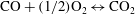 $\text{CO}+(1/2)\text{O}_{2}\leftrightarrow \text{CO}_{2}$
reaction (Peters & Williams Reference Peters and Williams1987; Franzelli et al.
Reference Franzelli, Riber, Gicquel and Poinsot2012). This may influence details of the expansion around the flame, and future work would be welcome to look at this point.
$\text{CO}+(1/2)\text{O}_{2}\leftrightarrow \text{CO}_{2}$
reaction (Peters & Williams Reference Peters and Williams1987; Franzelli et al.
Reference Franzelli, Riber, Gicquel and Poinsot2012). This may influence details of the expansion around the flame, and future work would be welcome to look at this point.
3. Flame diagnostics
In this section, the main parameters that will be used to understand the flame-base characteristics are introduced.
3.1. Scalar dissipation rate
The scalar dissipation rate can be used to examine the rate of molecular mixing and is also the key parameter in many models for turbulent non-premixed combustion. Some experimental and theoretical studies have shown that if the scalar dissipation is close to the ignition or extinction limits, dissipation effects can play an important role in determining the stabilisation location (Peters & Williams Reference Peters and Williams1983; Namazian et al. Reference Namazian, Schefer and Kelly1988; Müller et al. Reference Müller, Breitbach and Peters1994; Pitsch & Fedotov Reference Pitsch and Fedotov2000). The non-dimensional scalar dissipation rate is defined as
 $$\begin{eqnarray}{\it\chi}=\frac{2{\it\mu}}{{\it\rho}\mathit{Sc}}|\boldsymbol{{\rm\nabla}}Z|^{2}.\end{eqnarray}$$
3.2. Normalised flame index
The flame index (FI) representing the degree of mixedness was proposed by Yamashita, Shimada & Takeno (Reference Yamashita, Shimada and Takeno1996) to distinguish premixed from non-premixed flames. They defined the FI as a cosine of oxidiser and fuel gradient,
 $$\begin{eqnarray}\text{FI}=\boldsymbol{{\rm\nabla}}Y_{F}\boldsymbol{\cdot }\boldsymbol{{\rm\nabla}}Y_{O}.\end{eqnarray}$$
Domingo, Vervisch & Bray (Reference Domingo, Vervisch and Bray2002), Bray, Domingo & Vervisch (Reference Bray, Domingo and Vervisch2005), Domingo, Vervisch & Réveillon (Reference Domingo, Vervisch and Réveillon2005) and Knudsen & Pitsch (Reference Knudsen and Pitsch2012) have used a normalised flame index (NFI), defined as
 $$\begin{eqnarray}\text{NFI}=\frac{\boldsymbol{{\rm\nabla}}Y_{F}\boldsymbol{\cdot }\boldsymbol{{\rm\nabla}}Y_{O}}{|\boldsymbol{{\rm\nabla}}Y_{F}\boldsymbol{\cdot }\boldsymbol{{\rm\nabla}}Y_{O}|}.\end{eqnarray}$$
In areas that are burning (i.e. having a non-negligible reaction rate), the NFI can be used to determine the combustion mode. When the fuel and oxidiser gradients are aligned, this term is positive and indicates the presence of a premixed flame, while when these gradients are not aligned, the NFI will be negative, indicating the presence of a non-premixed flame.
To verify that the NFI can distinguish between premixed and non-premixed burning in this spatially developing flame, a steady laminar triple-flame case was run with the same chemistry parameters as the 3D DNS. Figure 7(a) shows the reaction rate of the product in the resulting triple-flame structure, with isolines of product mass fraction and mixture fraction overlaid for reference, while figure 7(b) shows the local NFI overlaid with the same isolines. It may be noted that the NFI successfully captures the leading premixed flame, which in this example has both lean and rich branches, and the trailing diffusion flame.

Figure 7. For a steady laminar triple flame with the same chemistry parameters as the DNS: (a) the reaction rate of the product in a laminar triple flame and (b) the NFI. In both plots, dashed curved lines show product mass-fraction isolines of 0.05, 0.1 and 0.2 while the solid lines show the stoichiometric mixture fraction and the mixture fraction
 $Z_{ms}$
0.07.
$Z_{ms}$
0.07.
3.3. Edge-flame identification and velocity
As stated in the introduction, one of the main objectives here is to analyse the edge-flame velocity. To achieve this, we first need to identify the flame base. Different approaches have been used for this purpose. In experimental studies of hydrocarbon flames, commencement of chemiluminescence of
 $\text{CH}^{\ast }$
(Su et al.
Reference Su, Sun and Mungal2006), CH PLIF (Watson et al.
Reference Watson, Lyons, Donbar and Carter2000; Hult et al.
Reference Hult, Meier, Meier, Harvey and Kaminski2005; Noda et al.
Reference Noda, Mori, Hongo and Nishioka2005; Lyons et al.
Reference Lyons, Watson, Carter and Donbar2007) or OH PLIF (Boxx et al.
Reference Boxx, Heeger, Gordon, Böhm, Aigner, Dreizler and Meier2009a
,Reference Boxx, Heeger, Gordon, Böhm, Dreizler and Meier
b
; Gordon et al.
Reference Gordon, Boxx, Carter, Dreizler and Meier2012) has frequently been used as the flame-base marker. The excited
$\text{CH}^{\ast }$
(Su et al.
Reference Su, Sun and Mungal2006), CH PLIF (Watson et al.
Reference Watson, Lyons, Donbar and Carter2000; Hult et al.
Reference Hult, Meier, Meier, Harvey and Kaminski2005; Noda et al.
Reference Noda, Mori, Hongo and Nishioka2005; Lyons et al.
Reference Lyons, Watson, Carter and Donbar2007) or OH PLIF (Boxx et al.
Reference Boxx, Heeger, Gordon, Böhm, Aigner, Dreizler and Meier2009a
,Reference Boxx, Heeger, Gordon, Böhm, Dreizler and Meier
b
; Gordon et al.
Reference Gordon, Boxx, Carter, Dreizler and Meier2012) has frequently been used as the flame-base marker. The excited
 $\text{CH}^{\ast }$
radical is short-lived and thought to mark the instantaneous reaction zone (Su et al.
Reference Su, Sun and Mungal2006). These locations coincide with high heat release rate.
$\text{CH}^{\ast }$
radical is short-lived and thought to mark the instantaneous reaction zone (Su et al.
Reference Su, Sun and Mungal2006). These locations coincide with high heat release rate.
In DNS of premixed flames, the high-heat-release region is often marked by a critical value of a reacting scalar (Echekki & Chen Reference Echekki and Chen1998; Im & Chen Reference Im and Chen1999; Tanahashi, Fujimura & Miyauchi Reference Tanahashi, Fujimura and Miyauchi2000; Im & Chen Reference Im and Chen2001; Chakraborty & Cant Reference Chakraborty and Cant2004; Hawkes & Chen Reference Hawkes and Chen2004, Reference Hawkes and Chen2006; Chen et al. Reference Chen, Hawkes, Sankaran, Mason and Im2006; Sankaran et al. Reference Sankaran, Hawkes, Chen, Lu and Law2006; Hawkes et al. Reference Hawkes, Sankaran, Sutherland and Chen2007c ). In our case, a more involved approach is needed since we wish to separate the edges from the region downstream. Following earlier studies of extinction and reignition (Pantano Reference Pantano2004; Hawkes, Sankaran & Chen Reference Hawkes, Sankaran and Chen2007a ,Reference Hawkes, Sankaran and Chen b ), we therefore select an edge-flame marker that is the intersection of a mixture-fraction isosurface and a product mass-fraction isosurface.
To select the mixture-fraction isovalue, it was first assumed that the leading edge would be found at the mixture fraction having the highest laminar flame speed,
 $Z_{ms}$
, which is slightly rich of stoichiometric (0.07 in this study, i.e.
$Z_{ms}$
, which is slightly rich of stoichiometric (0.07 in this study, i.e.
 $1.2Z_{st}$
). To select the product mass-fraction isosurface, a 1D simulation of a laminar premixed flame having the same flame parameters as the turbulent lifted flame was performed. The product mass fraction corresponding to the location of the maximum heat release rate was obtained from this simulation. The obtained value of
$1.2Z_{st}$
). To select the product mass-fraction isosurface, a 1D simulation of a laminar premixed flame having the same flame parameters as the turbulent lifted flame was performed. The product mass fraction corresponding to the location of the maximum heat release rate was obtained from this simulation. The obtained value of
 $Y_{p}$
was 0.2. To provide an example, these choices of mixture-fraction and product mass-fraction isosurfaces are marked on for the steady laminar triple flame shown in figure 7(a). It may be observed that the chosen parameters mark the peak reaction point at the leading edge of the flame quite well. Furthermore, a sensitivity study of the key results of these choices is presented in appendix B.
$Y_{p}$
was 0.2. To provide an example, these choices of mixture-fraction and product mass-fraction isosurfaces are marked on for the steady laminar triple flame shown in figure 7(a). It may be observed that the chosen parameters mark the peak reaction point at the leading edge of the flame quite well. Furthermore, a sensitivity study of the key results of these choices is presented in appendix B.
To extract the intersecting contour, the isosurface of the mixture fraction was triangulated with a parallel implementation of the marching-cubes algorithm. The edges of the resulting triangles were then searched for intersections with the product mass-fraction isosurface, and the intersection location was linearly estimated based on the vertex values of the product mass fraction. Quantities were then linearly interpolated to the intersection locations. It was verified that the mixture fraction and product mass fraction interpolated to the edge flames returned the expected values to typically within 1 %. The resulting edge-flame regions from the turbulent flame DNS were then extensively visualised and compared with locations of high heat release. It was found that the leading edge flame as identified visually from the reaction rate always remained very close to the intersection of the two isosurfaces.
Flame edges defined in this way can move by three mechanisms: flow, motion relative to the flow of the product mass-fraction isosurface and motion relative to the flow of the mixture-fraction isosurface. Although the velocity tangential to the flame edge could be arbitrarily specified, we take it to be equal to the flow velocity, following previous works on flame surface evolution (Pope Reference Pope1988) and on the tracking of extinction holes (Pantano Reference Pantano2004).
To determine the edge motion, we first need a coordinate system, which we take to be moving with the flow velocity. Referring to figure 8, we define a tangent vector to the mixture-fraction isosurfaces which points along the flame edge. The vector
 $\boldsymbol{T}_{1}$
is normal to both the normal to the mixture-fraction isosurface
$\boldsymbol{T}_{1}$
is normal to both the normal to the mixture-fraction isosurface
 $\boldsymbol{N}_{Z}$
(pointing towards the oxidiser) and to the normal to the product mass-fraction isosurface
$\boldsymbol{N}_{Z}$
(pointing towards the oxidiser) and to the normal to the product mass-fraction isosurface
 $\boldsymbol{N}_{Y_{p}}$
(pointing towards the reactants). Next, we define another vector
$\boldsymbol{N}_{Y_{p}}$
(pointing towards the reactants). Next, we define another vector
 $\boldsymbol{T}_{2}$
which is also tangential to the mixture-fraction isosurface but normal to
$\boldsymbol{T}_{2}$
which is also tangential to the mixture-fraction isosurface but normal to
 $\boldsymbol{T}_{1}$
, and pointing towards the reactants. It is readily shown that these quantities are given by
$\boldsymbol{T}_{1}$
, and pointing towards the reactants. It is readily shown that these quantities are given by
 $$\begin{eqnarray}\displaystyle \boldsymbol{N}_{Z} & = & \displaystyle -\frac{\boldsymbol{{\rm\nabla}}Z}{|\boldsymbol{{\rm\nabla}}Z|},\end{eqnarray}$$
 $$\begin{eqnarray}\displaystyle \boldsymbol{N}_{Y_{p}} & = & \displaystyle -\frac{\boldsymbol{{\rm\nabla}}Y_{p}}{|\boldsymbol{{\rm\nabla}}Y_{p}|},\end{eqnarray}$$
 $$\begin{eqnarray}\displaystyle \boldsymbol{T}_{1} & = & \displaystyle \frac{\boldsymbol{N}_{Y_{p}}\times \boldsymbol{N}_{Z}}{|\boldsymbol{N}_{Y_{p}}\times \boldsymbol{N}_{Z}|},\end{eqnarray}$$
 $$\begin{eqnarray}\displaystyle \boldsymbol{T}_{2} & = & \displaystyle \frac{\boldsymbol{N}_{Z}\times (\boldsymbol{N}_{Y_{p}}\times \boldsymbol{N}_{Z})}{|(\boldsymbol{N}_{Y_{p}}\times \boldsymbol{N}_{Z})|}\nonumber\\ \displaystyle & = & \displaystyle \frac{\boldsymbol{N}_{Y_{p}}-\boldsymbol{N}_{Z}(\boldsymbol{N}_{Y_{p}}\boldsymbol{\cdot }\boldsymbol{N}_{Z})}{\sqrt{1-(\boldsymbol{N}_{Y_{p}}\boldsymbol{\cdot }\boldsymbol{ N}_{Z})^{2}}}.\end{eqnarray}$$

Figure 8. The various normal and tangential vectors at the flame base: (a) schematic and (b) examples (the red–yellow surfaces are the product mass-fraction isosurfaces, the blue surfaces are the mixture-fraction isosurfaces and the solid black line is the identified edge flame).
Figure 9 now shows a schematic, in the plane containing both
 $\boldsymbol{N}_{Z}$
and
$\boldsymbol{N}_{Z}$
and
 $\boldsymbol{N}_{Y_{p}}$
, of the edge-flame motion during an infinitesimal interval of time
$\boldsymbol{N}_{Y_{p}}$
, of the edge-flame motion during an infinitesimal interval of time
 ${\it\delta}t$
. Because the chosen coordinate system moves with the local flow velocity, only the motion of the isosurfaces relative to the flow need be considered. During this time interval, the mixture-fraction isosurface is displaced by
${\it\delta}t$
. Because the chosen coordinate system moves with the local flow velocity, only the motion of the isosurfaces relative to the flow need be considered. During this time interval, the mixture-fraction isosurface is displaced by
 $S_{Z}\boldsymbol{N}_{Z}{\it\delta}t$
, while the
$S_{Z}\boldsymbol{N}_{Z}{\it\delta}t$
, while the
 $Y_{p}=Y_{p}^{\ast }$
isosurface is displaced by
$Y_{p}=Y_{p}^{\ast }$
isosurface is displaced by
 $S_{d}\boldsymbol{N}_{Y_{p}}{\it\delta}t$
, where the displacement speeds are given by (Gibson, Ashurst & Kerstein Reference Gibson, Ashurst and Kerstein1988; Pope Reference Pope1988; Echekki & Chen Reference Echekki and Chen1998)
$S_{d}\boldsymbol{N}_{Y_{p}}{\it\delta}t$
, where the displacement speeds are given by (Gibson, Ashurst & Kerstein Reference Gibson, Ashurst and Kerstein1988; Pope Reference Pope1988; Echekki & Chen Reference Echekki and Chen1998)
 $$\begin{eqnarray}\left.\begin{array}{@{}c@{}}\displaystyle S_{Z}=\frac{1}{{\it\rho}|\boldsymbol{{\rm\nabla}}Z|}\left(-\frac{\partial }{\partial \boldsymbol{x}_{j}}\left(\frac{{\it\mu}}{\mathit{Sc}}\frac{\partial Z}{\partial \boldsymbol{x}_{j}}\right)\right)\\ \displaystyle \text{and}\quad S_{d}=\frac{1}{{\it\rho}|\boldsymbol{{\rm\nabla}}Y_{P}|}\left(-\dot{{\it\omega}}_{P}-\frac{\partial }{\partial \boldsymbol{x}_{j}}\left(\frac{{\it\mu}}{\mathit{Sc}}\frac{\partial Y_{P}}{\partial \boldsymbol{x}_{j}}\right)\right),\end{array}\right\}\end{eqnarray}$$
where
 ${\it\mu}$
is the dynamic viscosity. We denote the overall displacement of the edge point
${\it\mu}$
is the dynamic viscosity. We denote the overall displacement of the edge point
 $\boldsymbol{V}_{e}{\it\delta}t$
and break this down into the orthonormal coordinates
$\boldsymbol{V}_{e}{\it\delta}t$
and break this down into the orthonormal coordinates
 $\boldsymbol{N}_{Z}$
and
$\boldsymbol{N}_{Z}$
and
 $\boldsymbol{T}_{2}$
as
$\boldsymbol{T}_{2}$
as
 $$\begin{eqnarray}\boldsymbol{V}_{e}{\it\delta}t=S_{z}\boldsymbol{N}_{Z}{\it\delta}t+S_{e}\boldsymbol{T}_{2}{\it\delta}t,\end{eqnarray}$$
where
 $S_{e}=\boldsymbol{V}_{e}\boldsymbol{\cdot }\boldsymbol{T}_{2}$
is the projection of
$S_{e}=\boldsymbol{V}_{e}\boldsymbol{\cdot }\boldsymbol{T}_{2}$
is the projection of
 $\boldsymbol{V}_{e}$
into the plane of the mixture-fraction isosurface and needs to be determined. Dividing by
$\boldsymbol{V}_{e}$
into the plane of the mixture-fraction isosurface and needs to be determined. Dividing by
 ${\it\delta}t$
, and taking the dot product of (3.9) with
${\it\delta}t$
, and taking the dot product of (3.9) with
 $\boldsymbol{N}_{Y_{p}}$
, it can be shown (noting that
$\boldsymbol{N}_{Y_{p}}$
, it can be shown (noting that
 $\boldsymbol{V}_{e}\boldsymbol{\cdot }\boldsymbol{N}_{Y_{p}}=S_{d}$
and using (3.8)) that
$\boldsymbol{V}_{e}\boldsymbol{\cdot }\boldsymbol{N}_{Y_{p}}=S_{d}$
and using (3.8)) that
 $$\begin{eqnarray}S_{e}=\frac{S_{d}-kS_{Z}}{\sqrt{1-k^{2}}},\end{eqnarray}$$
where
 $k$
is the inner product of the normal vectors
$k$
is the inner product of the normal vectors
 $\boldsymbol{N}_{Y_{p}}\boldsymbol{\cdot }\boldsymbol{N}_{Z}$
.
$\boldsymbol{N}_{Y_{p}}\boldsymbol{\cdot }\boldsymbol{N}_{Z}$
.

Figure 9. Schematic of edge-flame propagation along the mixture-fraction isosurface: (a) instantaneous vectors and indicative flame edge; (b) propagation of the edge point over an infinitesimal time interval
 ${\it\delta}t$
.
${\it\delta}t$
.
Although the presentation here is slightly different, we have verified that the final result is the same edge speed as used first by Pantano (Reference Pantano2004) to study extinction holes and later by Hawkes et al. (Reference Hawkes, Sankaran and Chen2007a ,Reference Hawkes, Sankaran and Chen b ) to study extinction and reignition, and also by Chakraborty & Mastorakos (Reference Chakraborty and Mastorakos2008) to study ignitions.
3.4. Out-of-plane motion
Many experimental investigations of lifted flames have used laser-based planar measurements (for example Wohl, Kapp & Gazley Reference Wohl, Kapp and Gazley1949; Vanquickenborne & van Tiggelen Reference Vanquickenborne and van Tiggelen1966; Kalghatgi Reference Kalghatgi1984; Namazian et al. Reference Namazian, Schefer and Kelly1988; Miake-Lye & Hammer Reference Miake-Lye and Hammer1989; Pitts Reference Pitts1989; Takahashi & Schmoll Reference Takahashi and Schmoll1991; Schefer et al. Reference Schefer, Namazian, Filtopoulos and Kelly1994a ,Reference Schefer, Namazian and Kelly b ; Muniz & Mungal Reference Muniz and Mungal1997; Schefer Reference Schefer1997a ,Reference Schefer b ; Hasselbrink & Mungal Reference Hasselbrink and Mungal1998; Kelman, Eltobaji & Masri Reference Kelman, Eltobaji and Masri1998; Schefer & Goix Reference Schefer and Goix1998; Tacke et al. Reference Tacke, Geyer, Hassel and Janicka1998; Takahashi, John Schmoll & Katta Reference Takahashi, John Schmoll and Katta1998; Brown, Watson & Lyons Reference Brown, Watson and Lyons1999; Watson et al. Reference Watson, Lyons, Donbar and Carter1999, Reference Watson, Lyons, Donbar and Carter2000, Reference Watson, Lyons, Carter and Donbar2002, Reference Watson, Lyons, Donbar and Carter2003; Han & Mungal Reference Han and Mungal2000; Maurey et al. Reference Maurey, Cessou, Lecordier and Stepowski2000; Baillot & Demare Reference Baillot and Demare2002; Mansour Reference Mansour2003, Reference Mansour2004; Noda et al. Reference Noda, Mori, Hongo and Nishioka2005), and therefore there have been numerous questions raised about out-of-plane motion and its potential role in flame stabilisation. Out-of-plane motion of the flame is the consequence of two effects: flow motion and flame propagation. The out-of-plane flow velocity has recently become accessible in cinema PIV experiments (e.g. Lyons et al. Reference Lyons, Watson, Carter and Donbar2007; Boxx et al. Reference Boxx, Heeger, Gordon, Böhm, Aigner, Dreizler and Meier2009a ,Reference Boxx, Heeger, Gordon, Böhm, Dreizler and Meier b ; Gordon et al. Reference Gordon, Boxx, Carter, Dreizler and Meier2012; Boxx, Meier & Carter Reference Boxx, Meier and Carter2014). The flame propagation component in the out-of-plane direction is, however, not available experimentally, and while out-of-plane flow can be measured, the flame orientation is unknown in the out-of-plane direction such that its effect is unknown. However, when DNS is used the three-dimensional (3D) flow field and the flame propagation are simultaneously available for such an analysis.
Consider an infinitesimally small flame-edge segment
 $\text{d}s(t)$
which is moving in the out-of-plane (spanwise,
$\text{d}s(t)$
which is moving in the out-of-plane (spanwise,
 $z$
) direction in a time
$z$
) direction in a time
 ${\it\delta}t$
to its new location
${\it\delta}t$
to its new location
 $\text{d}s(t+{\it\delta}t)$
. Over this period the point
$\text{d}s(t+{\it\delta}t)$
. Over this period the point
 $P(t)$
intersecting the
$P(t)$
intersecting the
 $x{-}y$
observation plane moves to location
$x{-}y$
observation plane moves to location
 $P(t+{\it\delta}t)$
causing an apparent in-plane motion unless the flame edge happens to be oriented normal to the
$P(t+{\it\delta}t)$
causing an apparent in-plane motion unless the flame edge happens to be oriented normal to the
 $x{-}y$
plane. (It also moves in the
$x{-}y$
plane. (It also moves in the
 $x{-}y$
plane due to flow and propagation in that plane, but here we adopt a coordinate system that follows that motion in order to simplify the discussion.) Figure 10 shows a schematic of this concept. It is readily observed that the observed flow speed (or flame propagation speed) in the plane is obtained by projecting the
$x{-}y$
plane due to flow and propagation in that plane, but here we adopt a coordinate system that follows that motion in order to simplify the discussion.) Figure 10 shows a schematic of this concept. It is readily observed that the observed flow speed (or flame propagation speed) in the plane is obtained by projecting the
 $z$
component of the flow velocity (or relative flame propagation velocity) into the
$z$
component of the flow velocity (or relative flame propagation velocity) into the
 $\boldsymbol{T}_{1}$
direction, then projecting the result into the
$\boldsymbol{T}_{1}$
direction, then projecting the result into the
 $x{-}y$
plane. We denote the apparent flow velocity by
$x{-}y$
plane. We denote the apparent flow velocity by
 $(\boldsymbol{U}_{z})_{x}$
and the apparent flame propagation by
$(\boldsymbol{U}_{z})_{x}$
and the apparent flame propagation by
 $(V_{e,z})_{x}$
(in the
$(V_{e,z})_{x}$
(in the
 $x$
direction here). It is readily shown that these velocities are given by
$x$
direction here). It is readily shown that these velocities are given by
 $$\begin{eqnarray}\displaystyle & (\boldsymbol{U}_{z})_{x}=-\boldsymbol{U}_{z}\tan ({\it\varphi})\cos ({\it\psi}), & \displaystyle\end{eqnarray}$$
 $$\begin{eqnarray}\displaystyle & (\boldsymbol{U}_{z})_{y}=-\boldsymbol{U}_{z}\tan ({\it\varphi})\sin ({\it\psi}), & \displaystyle\end{eqnarray}$$
 $$\begin{eqnarray}\displaystyle & (V_{e,z})_{x}=-V_{e,z}\tan ({\it\varphi})\cos ({\it\psi}) & \displaystyle\end{eqnarray}$$
 $$\begin{eqnarray}(V_{e,z})_{y}=-V_{e,z}\tan ({\it\varphi})\sin ({\it\psi}).\end{eqnarray}$$

Figure 10. Schematic of the displacement of the edge in the transverse and streamwise directions caused by out-of-plane motion.
4. Results and discussion
4.1. General flame structure
A volume rendering of the logarithm of the scalar dissipation rate normalised by the laminar flame time scale (blue/white) and reaction rate (red/orange) is presented in figure 11. Before reading further, the interested reader may consult an animation of the vorticity magnitude (blue/white) and reaction rate (red/orange) which is presented in the online supplementary movie to this paper available at http://dx.doi.org/10.1017/jfm.2015.334. This animation is quite instructive to gain an overall picture of the flame.
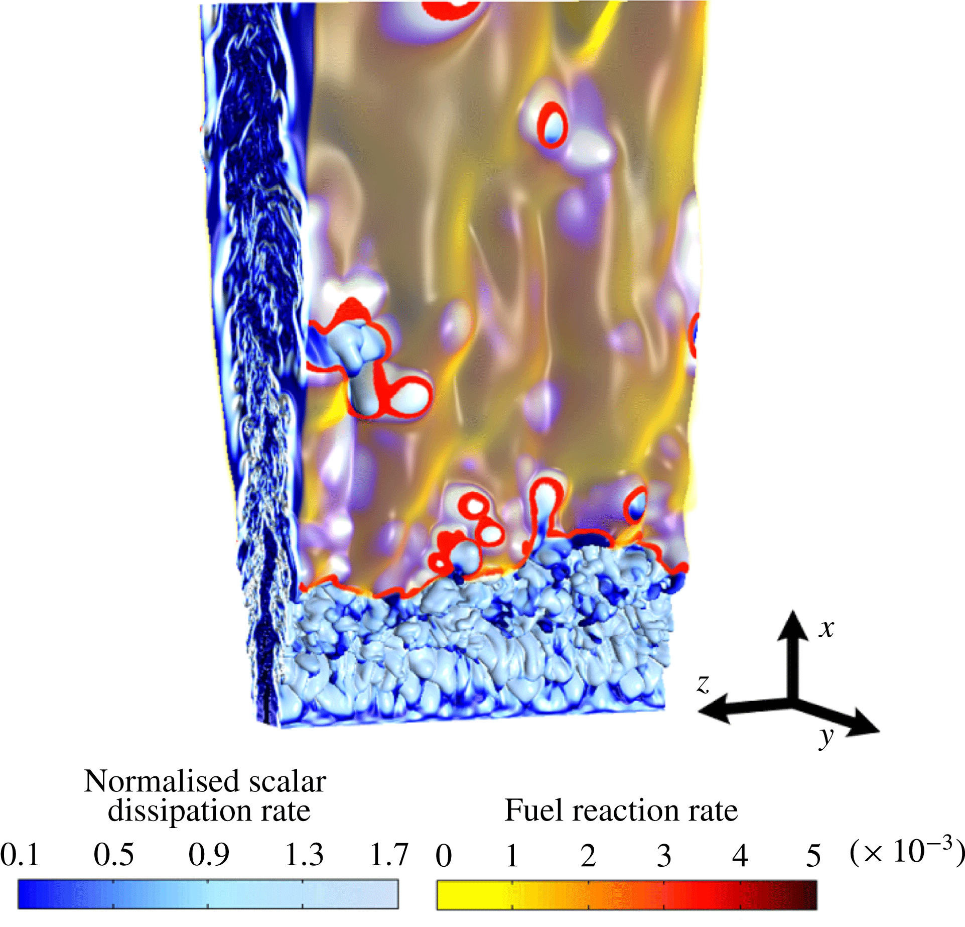
Figure 11. Three-dimensional volume rendering of the logarithm of the scalar dissipation rate (blue/white) and reaction rate (red/orange). (Only the region
 $x<14$
is shown.) Rendering generated by Dr Hongfeng Yu, using techniques described in Yu, Wang & Ma (Reference Yu, Wang and Ma2008); see also Akiba et al. (Reference Akiba, Ma, Chen and Hawkes2007).
$x<14$
is shown.) Rendering generated by Dr Hongfeng Yu, using techniques described in Yu, Wang & Ma (Reference Yu, Wang and Ma2008); see also Akiba et al. (Reference Akiba, Ma, Chen and Hawkes2007).
It may be observed in figure 11 that the flame has a complex structure which has features that are qualitatively similar to experimental observations of lifted flames (Schefer et al. Reference Schefer, Namazian and Kelly1994b ; Schefer Reference Schefer1997a ; Schefer & Goix Reference Schefer and Goix1998; Han & Mungal Reference Han and Mungal2000; Watson et al. Reference Watson, Lyons, Donbar and Carter2000; Hult et al. Reference Hult, Meier, Meier, Harvey and Kaminski2005; Joedicke et al. Reference Joedicke, Peters and Mansour2005; Boxx et al. Reference Boxx, Heeger, Gordon, Böhm, Aigner, Dreizler and Meier2009a ,Reference Boxx, Heeger, Gordon, Böhm, Dreizler and Meier b ). Because the stoichiometric mixture fraction is small (0.055), the flame is found at the edge of the highly turbulent inner core of the jet. Heat release noticeably damps turbulence in the outer region.
Unlike the DNS of lifted hydrogen flames reported by Mizobuchi et al. (Reference Mizobuchi, Tachibana, Shinio, Ogawa and Takeno2002, Reference Mizobuchi, Shinio, Ogawa and Takeno2005), we do not observe a vigorous rich premixed flame core. We believe that this difference is because hydrogen burns much more vigorously than hydrocarbons in rich mixtures. The mixture-fraction dependence of the burning velocity is built into the present model by the mixture-fraction-dependent activation energy. Similarly, we also did not observe any diffusion flame islands on the lean side that were observed by Mizobuchi et al. (Reference Mizobuchi, Tachibana, Shinio, Ogawa and Takeno2002, Reference Mizobuchi, Shinio, Ogawa and Takeno2005). The ‘islands’ noted by Mizobuchi et al. were regions of high hydrogen consumption rate which had a negative NFI, suggesting diffusion flame burning. Once again this might have been a hydrogen-specific feature since much of the hydrogen fuel was being consumed in the rich premixed branch, leaving little to be consumed in the diffusion flame. The authors note, however, that another reason for the observed differences is the larger lifted height observed in the Mizobuchi cases, which allowed a wider flammable region to form upstream of the lifted flame location. It is also possible, though considered unlikely by the authors, that the specific one-step mechanism adopted here can explain the differences between the two studies.
To further elaborate this essential difference between hydrocarbon and hydrogen lifted flames, figure 12 shows an isosurface of product reaction rate coloured by the NFI. It may be readily observed that the leading edges are premixed, followed by a trailing diffusion flame, which is mostly connected. Notably, there is not an extensive inner region of premixed flames, unlike in the case of hydrogen (Mizobuchi et al. Reference Mizobuchi, Tachibana, Shinio, Ogawa and Takeno2002, Reference Mizobuchi, Shinio, Ogawa and Takeno2005). Flame holes can be observed as the regions downstream of the leading edge, where high values of the NFI indicate a locally premixed edge. (Other holes are observed without being surrounded by premixed edges, but these are still diffusion flames, which just have a lower reaction rate than the chosen threshold.)

Figure 12. The reaction rate isosurface of fuel,
 $|\dot{{\it\omega}}_{F}|=0.001$
, coloured by the NFI.
$|\dot{{\it\omega}}_{F}|=0.001$
, coloured by the NFI.
Returning to the discussion of figure 11, the leading flame edges at the base of the flame are highly convoluted. Consistent with many experimental observations of lifted flames (Schefer et al. Reference Schefer, Namazian and Kelly1994b ; Schefer Reference Schefer1997a ; Schefer & Goix Reference Schefer and Goix1998; Han & Mungal Reference Han and Mungal2000; Watson et al. Reference Watson, Lyons, Donbar and Carter2000; Hult et al. Reference Hult, Meier, Meier, Harvey and Kaminski2005; Joedicke et al. Reference Joedicke, Peters and Mansour2005; Boxx et al. Reference Boxx, Heeger, Gordon, Böhm, Aigner, Dreizler and Meier2009a ,Reference Boxx, Heeger, Gordon, Böhm, Dreizler and Meier b ), the leading edges do not typically exhibit a tribrachial structure. This lack of three distinct branches has been previously explained to result from mixture-fraction gradients ahead of the flame being too large to support distinct lean and rich branches (Stårner et al. Reference Stårner, Bilger, Frank, Marran and Long1996). Occasionally, when the flame was found in a low-strain-rate region, we did observe a short or weak rich premixed branch, but a distinct lean branch was never observed.
The reaction rate is locally higher at the flame edges than further downstream, which is consistent with the existence of a premixed leading edge flame. It is also noted that in the present case, the premixed flame edges are quite narrow and of the order of the laminar flame thickness, which implies that the premixed edge flames are quite unlike a flat turbulent premixed flame with lateral dimensions much larger than the laminar flame thickness; i.e. at this lifted height, the premixed flame theory of stabilisation is ruled out, a fact that has already been noted by others, e.g. see the discussion in Lawn (Reference Lawn2009). In the authors’ interpretation of the premixed flame theory, as opposed to the edge-flame theory, the leading premixed flame has a lateral width that is significantly larger than the laminar flame thickness. In contrast, in the authors’ interpretation, the traditional edge-flame concept is only applicable if the lateral width is the order of at most a few laminar flame thicknesses.
There is a proliferation of flame holes, not observed in earlier DNS studies of lifted flames (Mizobuchi et al. Reference Mizobuchi, Tachibana, Shinio, Ogawa and Takeno2002, Reference Mizobuchi, Shinio, Ogawa and Takeno2005; Yoo et al. Reference Yoo, Sankaran and Chen2009, Reference Yoo, Richardson, Sankaran and Chen2011). In the case of Mizobuchi et al. (Reference Mizobuchi, Tachibana, Shinio, Ogawa and Takeno2002, Reference Mizobuchi, Shinio, Ogawa and Takeno2005), conversely to our situation, isolated burning islands in a mostly non-burning stoichiometric surface were observed rather than holes in a mostly connected burning surface. As will be presented in more detail shortly, these holes originate by two different mechanisms. Some of the holes are generated by flame propagation at the leading edge while others are caused by local flame extinction. Both kinds of holes can either grow or shrink and disappear as they go downstream. They can also merge with other holes and/or split into multiple holes. The existence of extinction holes suggests that in this flame (which has a relatively low lifted height) the critical scalar dissipation rate can be locally exceeded, which suggests that extinction can moderate the stabilisation process (Lyons et al. Reference Lyons, Watson, Carter and Donbar2007).
We do not, however, observe any unconnected regions of high reaction rate ahead of the leading edge. All regions ahead of the leading edge are connected, even though in a 2D streamwise–transverse plane they may appear as unconnected flame elements. (Although one still image cannot show this, the supplementary animations certainly do.) Nor do we observe any transport of hot products or even large-scale folding of the flame into upstream unburned regions. The lack of any unconnected regions or large-scale folding of the flame to upstream unburned regions therefore rules out, for the present flame, a stabilisation mechanism supported only by upstream turbulent transport. In an early theory, Broadwell et al. (Reference Broadwell, Dahm and Mungal1985) proposed that lateral ejection of hot products and later re-entrainment into the jet could support stabilisation of the flame at a given location, but nonetheless it seems to the present authors that some upstream transport mechanism would be needed in this theory to balance the oncoming flow once the flame is re-entrained into the high-streamwise-velocity region, and thus the present results seem to rule out this early theory.
The stabilisation mechanism is evidently far from being laminar in its overall structure. The large degree of convolution of the flame edge implies that it can consume stoichiometric reactants at a much greater rate than in a laminar flame (which would present a single straight line here), similar to how increased surface area causes the turbulent burning velocity to be larger than the laminar one in premixed flames. (It should be noted that, similar to a turbulent premixed flame, the existence of locally laminar structures is, however, not ruled out.) Another way of thinking about this in a planar picture of the flame is that out-of-plane motion can lead to additional upstream transport, i.e. that flames can propagate laterally around high-velocity regions in large eddies eventually leading to additional upstream propagation. Later in the article we will show that this mechanism is very significant in some regions of the flame.
It may be observed that the leading edge structure qualitatively seems to be convoluted on the scale of large eddies. The role of large eddies can also be qualitatively observed in the animation in the supplementary material. Later in the article we will present evidence that large eddies definitely do play a role in the stabilisation.
4.2. Scalar dissipation and hole formation
As mentioned earlier, some of the observed holes in the reaction sheet are a consequence of local extinctions which occur when high-scalar-dissipation-rate structures, with scalar dissipation rate comparable to the quenching limit, occur near the mixture-fraction isosurface. The scalar dissipation is a key parameter in many modelling frameworks, and some stabilisation theories have been developed on the critical scalar dissipation concept (Peters & Williams Reference Peters and Williams1983; Müller et al.
Reference Müller, Breitbach and Peters1994). To assess this theory and the qualitative observations in figure 11, instantaneous scatter plots of conditional normalised scalar dissipation rate on the mixture-fraction isosurface with the maximum laminar flame speed coloured by the product mass fraction at
 $t_{j}=11.55$
are presented in figure 13(a).
$t_{j}=11.55$
are presented in figure 13(a).

Figure 13. (a) Scatter plot of the logarithm of the scalar dissipation rate conditioned on the mixture-fraction isosurface
 $Z=0.07$
versus the distance from the nozzle and coloured by the product mass fraction for
$Z=0.07$
versus the distance from the nozzle and coloured by the product mass fraction for
 $t_{j}=11.55$
. (b) Scatter plot of the product mass fraction versus the logarithm of the scalar dissipation for
$t_{j}=11.55$
. (b) Scatter plot of the product mass fraction versus the logarithm of the scalar dissipation for
 $6.5<x<7.5$
.
$6.5<x<7.5$
.
There are a couple of interesting features to be noted in this figure. Both the scalar dissipation rate and its fluctuations are high upstream of the flame base. The high value of the logarithm of the normalised scalar dissipation rate (
 $\log _{10}({\it\chi}{\it\delta}_{L}/S_{L})$
) is more than unity, and as expected it decays in the streamwise direction. It is noticeably lower in the burning regions of the flame starting at approximately
$\log _{10}({\it\chi}{\it\delta}_{L}/S_{L})$
) is more than unity, and as expected it decays in the streamwise direction. It is noticeably lower in the burning regions of the flame starting at approximately
 $x/H\approx 3$
(as indicated by high product mass fractions) than in the upstream non-burning regions (as indicated by low product mass fractions). It may be noted that the highest dissipation rate regions correspond to the locations of holes (indicated by regions downstream of the lifted height but having a low product mass fraction). Connections between the scalar dissipation rate and local extinctions have been noted in several other DNS studies, e.g. Pantano (Reference Pantano2004), Hawkes et al. (Reference Hawkes, Sankaran and Chen2007b
) and Karami et al. (Reference Karami, Talei, Hawkes and Chatakonda2013), and in other models that can resolve such effects, e.g. Sen, Hawkes & Menon (Reference Sen, Hawkes and Menon2010) and Punati et al. (Reference Punati, Sutherland, Kerstein, Hawkes and Chen2011). This is confirmed in figure 13(b), which shows the product mass fraction on the same isosurface versus the scalar dissipation, conditioned on the locations
$x/H\approx 3$
(as indicated by high product mass fractions) than in the upstream non-burning regions (as indicated by low product mass fractions). It may be noted that the highest dissipation rate regions correspond to the locations of holes (indicated by regions downstream of the lifted height but having a low product mass fraction). Connections between the scalar dissipation rate and local extinctions have been noted in several other DNS studies, e.g. Pantano (Reference Pantano2004), Hawkes et al. (Reference Hawkes, Sankaran and Chen2007b
) and Karami et al. (Reference Karami, Talei, Hawkes and Chatakonda2013), and in other models that can resolve such effects, e.g. Sen, Hawkes & Menon (Reference Sen, Hawkes and Menon2010) and Punati et al. (Reference Punati, Sutherland, Kerstein, Hawkes and Chen2011). This is confirmed in figure 13(b), which shows the product mass fraction on the same isosurface versus the scalar dissipation, conditioned on the locations
 $6.5<x<7.5$
. Some regions of lower dissipation rate are also noted in holes. These are probably in holes that are reigniting, but also may be holes that are formed by another mechanism which is discussed below.
$6.5<x<7.5$
. Some regions of lower dissipation rate are also noted in holes. These are probably in holes that are reigniting, but also may be holes that are formed by another mechanism which is discussed below.
The structure of the observed holes is now identified and discussed in more detail using 3D visualisations. Figure 14 shows the same variables as figure 11 during the formation and reignition of an extinction hole. As shown in figure 14, the hole is formed in a region of high scalar dissipation rate which bulges out towards the oxidiser side. This appears to be connected with the passage of a large eddy. The hole is revealed to be significantly curved in the out-of-plane direction such that the high-scalar-dissipation region and thus the extinction hole has approximately similar streamwise and spanwise extents. As the large eddy passes, the scalar dissipation rate relaxes and the hole reignites.

Figure 14. Three-dimensional view of the creation and shrinking of an extinction hole. The same variables as in figure 11 are shown.

Figure 15. Three-dimensional time sequence of hole creation, showing the same variables as in figure 11.
The formation of a different type of hole is examined in figure 15. It is observed that initially there is a local downstream motion of the flame around a large eddy. This causes a horseshoe-like edge-flame structure to arise. In the subsequent frames the flame comes together in the upstream region, finally reconnecting to form a flame hole, which is termed here as an ‘inclusion hole’. If observed in a 2D
 $x{-}y$
plane, this would be seen as the appearance of an upstream island. The convergence of the flames on either side towards the reconnection point implies that flame propagation, and not simply out-of-plane advection, must be involved in the appearance of the upstream island in this case. Thus, the present work demonstrates two distinct mechanisms of hole formation, and a connection of the appearance of some upstream islands (as observed in a plane) with the formation of an inclusion hole. Importantly, both of these mechanisms generate mixture-fraction conditional fluctuations of temperature and species, which may be important to represent from a modelling perspective. In planar experimental measurements it is impossible to definitely determine which mechanism causes the observed holes, because holes can be created by out-of-plane motion of reacting regions into the plane or by out-of-plane motion of non-reacting regions into the plane. However, a very recent study by Boxx et al. (Reference Boxx, Meier and Carter2014) used a combination of OH PLIF and line-of-sight OH* chemiluminescence to suggest that there can be very significant out-of-plane flame-edge wrinkling, such that apparently observed in-plane holes are actually not holes but are connected to the main leading edge of the flame, which is consistent with our observations in this DNS.
$x{-}y$
plane, this would be seen as the appearance of an upstream island. The convergence of the flames on either side towards the reconnection point implies that flame propagation, and not simply out-of-plane advection, must be involved in the appearance of the upstream island in this case. Thus, the present work demonstrates two distinct mechanisms of hole formation, and a connection of the appearance of some upstream islands (as observed in a plane) with the formation of an inclusion hole. Importantly, both of these mechanisms generate mixture-fraction conditional fluctuations of temperature and species, which may be important to represent from a modelling perspective. In planar experimental measurements it is impossible to definitely determine which mechanism causes the observed holes, because holes can be created by out-of-plane motion of reacting regions into the plane or by out-of-plane motion of non-reacting regions into the plane. However, a very recent study by Boxx et al. (Reference Boxx, Meier and Carter2014) used a combination of OH PLIF and line-of-sight OH* chemiluminescence to suggest that there can be very significant out-of-plane flame-edge wrinkling, such that apparently observed in-plane holes are actually not holes but are connected to the main leading edge of the flame, which is consistent with our observations in this DNS.
4.3. Time evolution of the flame base
To demonstrate some key features of the motion of flame edges, and to relate these features to previously observed experimental measurements in 2D planes, this section considers observations of the edge-flame motion at an arbitrarily selected plane at
 $z=0$
. Where it results in significant effects, out-of-plane motion of the flame is also considered.
$z=0$
. Where it results in significant effects, out-of-plane motion of the flame is also considered.
A time series of the most upstream flame-edge location is presented in figure 16 at the
 $z=0$
plane. The flame edge was identified as the intersection of mixture-fraction and product mass-fraction isosurfaces as discussed in § 3.3, and when more than one such location appeared in a plane, the most upstream was selected. The mean stabilisation point is
$z=0$
plane. The flame edge was identified as the intersection of mixture-fraction and product mass-fraction isosurfaces as discussed in § 3.3, and when more than one such location appeared in a plane, the most upstream was selected. The mean stabilisation point is
 $3.2H$
in the streamwise direction. Fluctuations of the order of the jet width can occur in the streamwise direction. The mean transverse location is
$3.2H$
in the streamwise direction. Fluctuations of the order of the jet width can occur in the streamwise direction. The mean transverse location is
 $-1.2H$
. The maximum level of fluctuations is less than
$-1.2H$
. The maximum level of fluctuations is less than
 $0.5H$
in the transverse direction.
$0.5H$
in the transverse direction.

Figure 16. Temporal evolution of (a) the streamwise location and (b) the transverse location at the most upstream flame edge on the plane
 $z=0$
.
$z=0$
.
Several different events involving upstream and downstream motion are noted in figure 16. At times there is smooth downstream (
 $P_{1},P_{3}$
) and upstream (
$P_{1},P_{3}$
) and upstream (
 $P_{2}$
) motion, but also at times there are sudden jumps in the lifted height (
$P_{2}$
) motion, but also at times there are sudden jumps in the lifted height (
 $P_{5}$
). According to the literature, the upstream jumps are expected to be related to out-of-plane motion (Lyons et al.
Reference Lyons, Watson, Carter and Donbar2007; Boxx et al.
Reference Boxx, Heeger, Gordon, Böhm, Aigner, Dreizler and Meier2009a
,Reference Boxx, Heeger, Gordon, Böhm, Dreizler and Meier
b
; Gordon et al.
Reference Gordon, Boxx, Carter, Dreizler and Meier2012) or conceivably to the appearance of isolated islands (Broadwell et al.
Reference Broadwell, Dahm and Mungal1985; Mizobuchi et al.
Reference Mizobuchi, Tachibana, Shinio, Ogawa and Takeno2002, Reference Mizobuchi, Shinio, Ogawa and Takeno2005). Sudden downstream motions of the flame base are also observed. Examples of different flame motion scenarios marked in figure 16 are now discussed in more detail, whereas the probability of their occurrence is discussed in a later section of the paper.
$P_{5}$
). According to the literature, the upstream jumps are expected to be related to out-of-plane motion (Lyons et al.
Reference Lyons, Watson, Carter and Donbar2007; Boxx et al.
Reference Boxx, Heeger, Gordon, Böhm, Aigner, Dreizler and Meier2009a
,Reference Boxx, Heeger, Gordon, Böhm, Dreizler and Meier
b
; Gordon et al.
Reference Gordon, Boxx, Carter, Dreizler and Meier2012) or conceivably to the appearance of isolated islands (Broadwell et al.
Reference Broadwell, Dahm and Mungal1985; Mizobuchi et al.
Reference Mizobuchi, Tachibana, Shinio, Ogawa and Takeno2002, Reference Mizobuchi, Shinio, Ogawa and Takeno2005). Sudden downstream motions of the flame base are also observed. Examples of different flame motion scenarios marked in figure 16 are now discussed in more detail, whereas the probability of their occurrence is discussed in a later section of the paper.

Figure 17. Time evolution of the flame base in the plane
 $z=0$
during the time period
$z=0$
during the time period
 $P_{1}$
, exhibiting smooth downstream motion when the apparent streamwise velocity and streamwise component of the edge velocity are positive. (a) The reaction rate on a colour scale, with vorticity contours in blue and red solid lines marking the flammability limits (laminar flame speed less than 5 % of maximum 1D laminar flame speed). (b) The logarithm of the scalar dissipation rate. (c) The apparent flow and propagation velocity vector components. In all panels the black solid line marks the product mass fraction of 0.2 while the dashed line is the mixture fraction of 0.07.
$P_{1}$
, exhibiting smooth downstream motion when the apparent streamwise velocity and streamwise component of the edge velocity are positive. (a) The reaction rate on a colour scale, with vorticity contours in blue and red solid lines marking the flammability limits (laminar flame speed less than 5 % of maximum 1D laminar flame speed). (b) The logarithm of the scalar dissipation rate. (c) The apparent flow and propagation velocity vector components. In all panels the black solid line marks the product mass fraction of 0.2 while the dashed line is the mixture fraction of 0.07.
Figure 17 presents, for the time period
 $P_{1}$
, (a) contours of the reaction rate and vorticity magnitude, (b) contours of the logarithm of the normalised scalar dissipation rate and (c) the streamwise and transverse vector components of the apparent flow and edge-flame propagation velocities at the flame-base location. The black solid line represents the product mass fraction of 0.2 and the dashed line corresponds to the mixture fraction of 0.07, which has the maximum laminar flame speed. (Recall that the intersection of these isosurfaces defines the ‘flame edge’. It may be noted that they do indeed provide a good marker in the forthcoming figures.) The two red solid lines in figure 17(a) indicate the flammability limits. The lower and upper flammability limits of methane are
$P_{1}$
, (a) contours of the reaction rate and vorticity magnitude, (b) contours of the logarithm of the normalised scalar dissipation rate and (c) the streamwise and transverse vector components of the apparent flow and edge-flame propagation velocities at the flame-base location. The black solid line represents the product mass fraction of 0.2 and the dashed line corresponds to the mixture fraction of 0.07, which has the maximum laminar flame speed. (Recall that the intersection of these isosurfaces defines the ‘flame edge’. It may be noted that they do indeed provide a good marker in the forthcoming figures.) The two red solid lines in figure 17(a) indicate the flammability limits. The lower and upper flammability limits of methane are
 ${\it\phi}=0.46$
and 1.64 respectively (Dahoe & De Goey Reference Dahoe and De Goey2003). These limits correspond to the laminar flame speed being less than approximately 5 % of the maximum laminar flame speed. The time sequences are presented from left to right. The fuel and oxidiser are on the left- and right-hand sides respectively. As can be seen, at times
${\it\phi}=0.46$
and 1.64 respectively (Dahoe & De Goey Reference Dahoe and De Goey2003). These limits correspond to the laminar flame speed being less than approximately 5 % of the maximum laminar flame speed. The time sequences are presented from left to right. The fuel and oxidiser are on the left- and right-hand sides respectively. As can be seen, at times
 $t_{j}=11.49$
and 11.55 large eddies squeeze the flammable region (figure 17(a), marked as
$t_{j}=11.49$
and 11.55 large eddies squeeze the flammable region (figure 17(a), marked as
 $A_{P1}$
). This results in a comet-shaped flame front as marked by
$A_{P1}$
). This results in a comet-shaped flame front as marked by
 $B_{P1}$
in figure 17(a). As shown in figure 17(b), the scalar dissipation rate is also high at the flame base (marked as
$B_{P1}$
in figure 17(a). As shown in figure 17(b), the scalar dissipation rate is also high at the flame base (marked as
 $C_{P1}$
). In this case, the dissipation rate is high enough to cause a positive apparent propagation velocity, i.e. a negative relative flame speed, noting that the flame normal is pointing towards the negative streamwise direction. In the next two time sequences,
$C_{P1}$
). In this case, the dissipation rate is high enough to cause a positive apparent propagation velocity, i.e. a negative relative flame speed, noting that the flame normal is pointing towards the negative streamwise direction. In the next two time sequences,
 $t_{j}=11.64$
and 11.70, there is no large structure in the vicinity of the flame base and the scalar dissipation begins to relax, leading to less negative relative flame speeds by
$t_{j}=11.64$
and 11.70, there is no large structure in the vicinity of the flame base and the scalar dissipation begins to relax, leading to less negative relative flame speeds by
 $t_{j}=11.76$
. As a result, the flame speed becomes positive again and approximately balances the flow (figure 17
c).
$t_{j}=11.76$
. As a result, the flame speed becomes positive again and approximately balances the flow (figure 17
c).
Figure 17(c) also presents the apparent transverse propagation and flow velocities by orange and dark blue horizontal vectors respectively. It shows that the flame propagates relative to the flow towards the region of leaner mixtures and is dominant over the entrainment flow directing the flame towards the region of richer mixtures. It is noted that at times
 $t_{j}=11.70$
and 11.76 (as can be seen in figure 17
a) a small and weak reaction zone appears upstream of the flame base which is caused by out-of-plane motion. This effect will be analysed in more detail later in this section.
$t_{j}=11.70$
and 11.76 (as can be seen in figure 17
a) a small and weak reaction zone appears upstream of the flame base which is caused by out-of-plane motion. This effect will be analysed in more detail later in this section.
During the time period
 $P_{2}$
, a case of upstream propagation is presented in figure 18. Once again, the same parameters as in figure 17 are shown. As shown in figure 18(a), at time
$P_{2}$
, a case of upstream propagation is presented in figure 18. Once again, the same parameters as in figure 17 are shown. As shown in figure 18(a), at time
 $t_{j}=15.63$
the flammable region is wide, approximately twice as wide as the laminar flame thickness. There are no large eddies containing vortical fluid around the flame base to disturb the propagation process. The absence of such structures also allows the existence of a rich premixed wing. The scalar dissipation rate is low in a large region upstream of the flame base. All of these conditions are favourable for flame propagation, and as a result the upstream propagation speed of the flame is strong, as shown in figure 18(c). Due to the subsequent passage of a large eddy, the thickness of the flammable region decreases and the scalar dissipation rate increases, which leads to the upstream propagation speed decreasing. At approximately
$t_{j}=15.63$
the flammable region is wide, approximately twice as wide as the laminar flame thickness. There are no large eddies containing vortical fluid around the flame base to disturb the propagation process. The absence of such structures also allows the existence of a rich premixed wing. The scalar dissipation rate is low in a large region upstream of the flame base. All of these conditions are favourable for flame propagation, and as a result the upstream propagation speed of the flame is strong, as shown in figure 18(c). Due to the subsequent passage of a large eddy, the thickness of the flammable region decreases and the scalar dissipation rate increases, which leads to the upstream propagation speed decreasing. At approximately
 $t_{j}=15.87$
the dissipation rate relaxes and the upstream flame propagation speed increases again.
$t_{j}=15.87$
the dissipation rate relaxes and the upstream flame propagation speed increases again.

Figure 18. Time evolution of the flame base on the plane
 $z=0$
for a case involving a smooth upstream propagation during period
$z=0$
for a case involving a smooth upstream propagation during period
 $P_{2}$
. (a) The reaction rate on a colour scale, with vorticity contours in blue and the red solid lines marking the flammability limits. (b) The logarithm of the scalar dissipation rate. (c) The apparent flow and propagation velocity vector components. In all panels the black solid line marks the product mass fraction of 0.2 while the dashed line is the mixture fraction of 0.07.
$P_{2}$
. (a) The reaction rate on a colour scale, with vorticity contours in blue and the red solid lines marking the flammability limits. (b) The logarithm of the scalar dissipation rate. (c) The apparent flow and propagation velocity vector components. In all panels the black solid line marks the product mass fraction of 0.2 while the dashed line is the mixture fraction of 0.07.
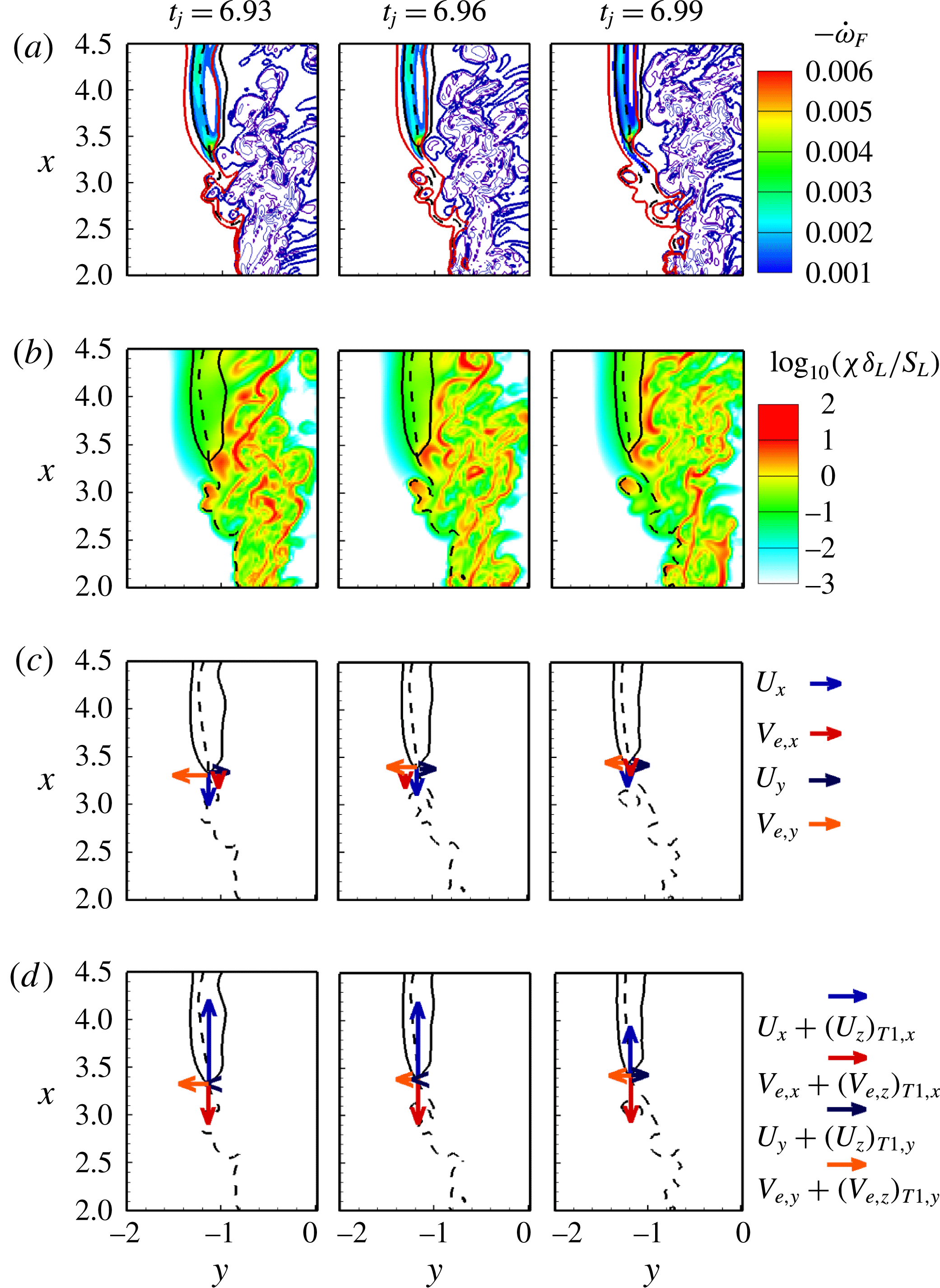
Figure 19. Time evolution of the flame base at the plane
 $z=0$
for a case of smooth downstream motion during time period
$z=0$
for a case of smooth downstream motion during time period
 $P_{3}$
when the apparent streamwise velocity and streamwise component of the edge velocity are negative. (a) The reaction rate on a colour scale, with the contours of vorticity magnitude in blue and the red solid lines marking the flammability limits. (b) The logarithm of the scalar dissipation rate. (c) The streamwise and transverse flow and edge propagation velocity vector components. (d) The apparent flow and propagation velocity vector components. In all panels the black solid line marks the product mass fraction of 0.2 while the dashed line is the mixture fraction of 0.07.
$P_{3}$
when the apparent streamwise velocity and streamwise component of the edge velocity are negative. (a) The reaction rate on a colour scale, with the contours of vorticity magnitude in blue and the red solid lines marking the flammability limits. (b) The logarithm of the scalar dissipation rate. (c) The streamwise and transverse flow and edge propagation velocity vector components. (d) The apparent flow and propagation velocity vector components. In all panels the black solid line marks the product mass fraction of 0.2 while the dashed line is the mixture fraction of 0.07.

Figure 20. Temporal snapshots during the event
 $P_{4}$
involving the appearance of a hook shape. (a) Contours of the reaction rate on a colour scale, with vorticity contours in blue. (b) Contours of the logarithm of scalar dissipation. (c) Flow and flame propagation velocity vector components. In all panels the black solid line marks the product mass fraction of 0.2 while the dashed line is the mixture fraction of 0.07.
$P_{4}$
involving the appearance of a hook shape. (a) Contours of the reaction rate on a colour scale, with vorticity contours in blue. (b) Contours of the logarithm of scalar dissipation. (c) Flow and flame propagation velocity vector components. In all panels the black solid line marks the product mass fraction of 0.2 while the dashed line is the mixture fraction of 0.07.
The time period
 $P_{3}$
shown in figure 16 is considered now. Figure 19(a,b) presents the same variables as previously shown in figure 17(a,b). Figure 19(c) shows the in-plane flow and edge-flame propagation velocities and figure 19(d) shows the apparent flow and flame propagation velocities with the out-of-plane component included. In contrast to the previous downstream motion shown in figure 17, this case features a much wider flammable region (with a weak rich premixed branch being evident) and a lower scalar dissipation rate, and as a result the flame speed is positive, which according to the in-plane picture would lead to an upstream propagation, since the flow velocity is also in the upstream direction. However, when the out-of-plane components are added in, the picture is rather different. While the upstream flame propagation is stronger with the inclusion of the out-of-plane propagation, inclusion of the
$P_{3}$
shown in figure 16 is considered now. Figure 19(a,b) presents the same variables as previously shown in figure 17(a,b). Figure 19(c) shows the in-plane flow and edge-flame propagation velocities and figure 19(d) shows the apparent flow and flame propagation velocities with the out-of-plane component included. In contrast to the previous downstream motion shown in figure 17, this case features a much wider flammable region (with a weak rich premixed branch being evident) and a lower scalar dissipation rate, and as a result the flame speed is positive, which according to the in-plane picture would lead to an upstream propagation, since the flow velocity is also in the upstream direction. However, when the out-of-plane components are added in, the picture is rather different. While the upstream flame propagation is stronger with the inclusion of the out-of-plane propagation, inclusion of the
 $z$
component of the flow velocity results in an even larger downstream apparent velocity, thus demonstrating that out-of-plane motion definitely needs to be considered in the overall picture.
$z$
component of the flow velocity results in an even larger downstream apparent velocity, thus demonstrating that out-of-plane motion definitely needs to be considered in the overall picture.
Before moving on, it is remarked that we also observed nearly every other combination of different components (flow/flame and in-plane/out-of-plane) being dominant. The above cases were selected only to provide some examples, and should not be interpreted as the statistically most significant situations. The statistically averaged picture is discussed later in the article.
Figure 20 shows an example that involves a large transverse velocity resulting in the creation of a hook structure (time period
 $P_{4}$
in figure 16). The variables shown are once again the same as in figure 17. At
$P_{4}$
in figure 16). The variables shown are once again the same as in figure 17. At
 $t_{j}=14.94$
the flame initially has a fairly unconvoluted structure which is propagating towards the fuel side. At the second time instant shown a large turbulent eddy bulges out towards the oxidiser side, which may be observed at the point marked ‘
$t_{j}=14.94$
the flame initially has a fairly unconvoluted structure which is propagating towards the fuel side. At the second time instant shown a large turbulent eddy bulges out towards the oxidiser side, which may be observed at the point marked ‘
 $A_{P4}$
’, where the high-vorticity region impinges onto the flame from the oxidiser side. At the same time, a large entrainment flow is occurring at the base. The coupling of the bulging turbulent eddy and the entraining flow causes an anticlockwise rotation of the flame and distorts it into a ‘hook’ structure. Such hook structures have been observed frequently in experimental measurements of lifted flames (for instance figure 7 in Kelman et al. (Reference Kelman, Eltobaji and Masri1998), figure 3(a) in Schefer et al. (Reference Schefer, Namazian and Kelly1994b
), figures 3(f) and 4(a) in Watson et al. (Reference Watson, Lyons, Donbar and Carter2000), figure 4 in Upatnieks, Driscoll & Ceccio (Reference Upatnieks, Driscoll and Ceccio2002), figure 5 in Boxx et al. (Reference Boxx, Heeger, Gordon, Böhm, Aigner, Dreizler and Meier2009a
), figure 4 in Boxx et al. (Reference Boxx, Heeger, Gordon, Böhm, Dreizler and Meier2009b
) and figure 3 in Gordon et al. (Reference Gordon, Boxx, Carter, Dreizler and Meier2012)) and are confirmed by the present DNS. The role played by large eddies in the creation of these structures supports the schematic of Kelman et al. (Reference Kelman, Eltobaji and Masri1998), and is consistent with experimental measurements by Upatnieks et al. (Reference Upatnieks, Driscoll and Ceccio2002, Reference Upatnieks, Driscoll, Rasmussen and Ceccio2004) and Boxx et al. (Reference Boxx, Heeger, Gordon, Böhm, Aigner, Dreizler and Meier2009a
,Reference Boxx, Heeger, Gordon, Böhm, Dreizler and Meier
b
). In the example shown here, the large eddy is even strong enough to cause an extinction hole above the leading edge location.
$A_{P4}$
’, where the high-vorticity region impinges onto the flame from the oxidiser side. At the same time, a large entrainment flow is occurring at the base. The coupling of the bulging turbulent eddy and the entraining flow causes an anticlockwise rotation of the flame and distorts it into a ‘hook’ structure. Such hook structures have been observed frequently in experimental measurements of lifted flames (for instance figure 7 in Kelman et al. (Reference Kelman, Eltobaji and Masri1998), figure 3(a) in Schefer et al. (Reference Schefer, Namazian and Kelly1994b
), figures 3(f) and 4(a) in Watson et al. (Reference Watson, Lyons, Donbar and Carter2000), figure 4 in Upatnieks, Driscoll & Ceccio (Reference Upatnieks, Driscoll and Ceccio2002), figure 5 in Boxx et al. (Reference Boxx, Heeger, Gordon, Böhm, Aigner, Dreizler and Meier2009a
), figure 4 in Boxx et al. (Reference Boxx, Heeger, Gordon, Böhm, Dreizler and Meier2009b
) and figure 3 in Gordon et al. (Reference Gordon, Boxx, Carter, Dreizler and Meier2012)) and are confirmed by the present DNS. The role played by large eddies in the creation of these structures supports the schematic of Kelman et al. (Reference Kelman, Eltobaji and Masri1998), and is consistent with experimental measurements by Upatnieks et al. (Reference Upatnieks, Driscoll and Ceccio2002, Reference Upatnieks, Driscoll, Rasmussen and Ceccio2004) and Boxx et al. (Reference Boxx, Heeger, Gordon, Böhm, Aigner, Dreizler and Meier2009a
,Reference Boxx, Heeger, Gordon, Böhm, Dreizler and Meier
b
). In the example shown here, the large eddy is even strong enough to cause an extinction hole above the leading edge location.
These upstream and downstream motions of the edge flame at the
 $z=0$
plane suggest that the edge flames might go through a cyclic motion. Therefore, the trajectories of the edge flames for the time periods when no island is observed in the
$z=0$
plane suggest that the edge flames might go through a cyclic motion. Therefore, the trajectories of the edge flames for the time periods when no island is observed in the
 $z=0$
plane will reveal this. Three different examples of cyclic motions are presented in figure 21. However, as this analysis is limited to the
$z=0$
plane will reveal this. Three different examples of cyclic motions are presented in figure 21. However, as this analysis is limited to the
 $z=0$
plane, excluding the out-of-plane jumps, more investigation on the overall behaviour of the flame base is needed. This will be discussed in more detail in the forthcoming sections.
$z=0$
plane, excluding the out-of-plane jumps, more investigation on the overall behaviour of the flame base is needed. This will be discussed in more detail in the forthcoming sections.

Figure 21. Instantaneous trajectory of the flame base at the plane
 $z=0.0$
.
$z=0.0$
.
The appearance of flame islands upstream of the main flame has been observed in many experimental studies of lifted flames (Upatnieks et al. Reference Upatnieks, Driscoll and Ceccio2002; Lyons et al. Reference Lyons, Watson, Carter and Donbar2007; Boxx et al. Reference Boxx, Heeger, Gordon, Böhm, Aigner, Dreizler and Meier2009a ,Reference Boxx, Heeger, Gordon, Böhm, Dreizler and Meier b , Reference Boxx, Meier and Carter2014; Gordon et al. Reference Gordon, Boxx, Carter, Dreizler and Meier2012). The laser-based diagnostic techniques used in these studies rely on measurements in 2D sheets. To analyse the effect of the out-of-plane motion on flame stabilisation, access to both the out-of-plane flow and the flame propagation velocities is necessary, which has not yet been demonstrated experimentally. However, DNS provides the full 3D data, which allows for a detailed examination of the out-of-plane flame motion. In this section, an example of the appearance of a flame island near the flame base is presented. The effects of flow and flame propagation are also investigated.
Figure 22 shows the contour plots of the out-of-plane (spanwise) flow velocity. At
 $t_{j}=14.13$
a small island appears in a region where the out-of-plane velocity is positive. This island (marked as
$t_{j}=14.13$
a small island appears in a region where the out-of-plane velocity is positive. This island (marked as
 $A_{P5}$
) grows rapidly, as can be seen in the next time,
$A_{P5}$
) grows rapidly, as can be seen in the next time,
 $t_{j}=14.28$
and 14.31. At
$t_{j}=14.28$
and 14.31. At
 $t_{j}=14.34$
the island disappears. The appearance of islands in the observation plane has been reported in many experimental studies of lifted flames (Upatnieks et al.
Reference Upatnieks, Driscoll and Ceccio2002; Lyons et al.
Reference Lyons, Watson, Carter and Donbar2007; Boxx et al.
Reference Boxx, Heeger, Gordon, Böhm, Aigner, Dreizler and Meier2009a
,Reference Boxx, Heeger, Gordon, Böhm, Dreizler and Meier
b
, Reference Boxx, Meier and Carter2014; Gordon et al.
Reference Gordon, Boxx, Carter, Dreizler and Meier2012); however, the inaccessible third dimension in the experiments has limited investigations of the physical reasons for the observed islands. It has been suggested that islands can result from either propagation or convective motion of the flame edge from the negative
$t_{j}=14.34$
the island disappears. The appearance of islands in the observation plane has been reported in many experimental studies of lifted flames (Upatnieks et al.
Reference Upatnieks, Driscoll and Ceccio2002; Lyons et al.
Reference Lyons, Watson, Carter and Donbar2007; Boxx et al.
Reference Boxx, Heeger, Gordon, Böhm, Aigner, Dreizler and Meier2009a
,Reference Boxx, Heeger, Gordon, Böhm, Dreizler and Meier
b
, Reference Boxx, Meier and Carter2014; Gordon et al.
Reference Gordon, Boxx, Carter, Dreizler and Meier2012); however, the inaccessible third dimension in the experiments has limited investigations of the physical reasons for the observed islands. It has been suggested that islands can result from either propagation or convective motion of the flame edge from the negative
 $z$
direction. To examine this hypothesis, the
$z$
direction. To examine this hypothesis, the
 $x{-}z$
plane view of the flame base is presented in figure 23. Shown here, the flame base is a continuous structure and there is no disconnected pocket of product or reaction zone upstream of the flame base. Instead, the island is observed in the
$x{-}z$
plane view of the flame base is presented in figure 23. Shown here, the flame base is a continuous structure and there is no disconnected pocket of product or reaction zone upstream of the flame base. Instead, the island is observed in the
 $x{-}y$
plane due to contortion and motion of the edge. (We also reiterate at this point that we never observed any disconnected upstream islands in the 3D animations of this case.) In figure 23, the flame base is also coloured by (a) spanwise velocity and (b) spanwise edge base propagation. At
$x{-}y$
plane due to contortion and motion of the edge. (We also reiterate at this point that we never observed any disconnected upstream islands in the 3D animations of this case.) In figure 23, the flame base is also coloured by (a) spanwise velocity and (b) spanwise edge base propagation. At
 $t_{j}=14.13$
, while the out-of-plane velocity is positive, the out-of-plane propagation exceeds the flow and is in the opposite direction, leading to the flame island actually appearing from the opposite side as suggested by the flow alone. Eventually, the out-of-plane flow reverses and both components promote growth of the island in the
$t_{j}=14.13$
, while the out-of-plane velocity is positive, the out-of-plane propagation exceeds the flow and is in the opposite direction, leading to the flame island actually appearing from the opposite side as suggested by the flow alone. Eventually, the out-of-plane flow reverses and both components promote growth of the island in the
 $x{-}y$
plane. We also observed cases of the opposite scenario, and cases when the flow and flame velocities were aligned and not aligned. However, overall, the results certainly suggest that flame propagation in the out-of-plane direction cannot be ignored. Planned future work will quantify in an averaged sense the role of out-of-plane flow and flame propagation on the appearance of upstream islands, as well as quantifying other out-of-plane effects in an effort to better understand the existing very substantial body of experimental work based on in-plane measurements.
$x{-}y$
plane. We also observed cases of the opposite scenario, and cases when the flow and flame velocities were aligned and not aligned. However, overall, the results certainly suggest that flame propagation in the out-of-plane direction cannot be ignored. Planned future work will quantify in an averaged sense the role of out-of-plane flow and flame propagation on the appearance of upstream islands, as well as quantifying other out-of-plane effects in an effort to better understand the existing very substantial body of experimental work based on in-plane measurements.

Figure 22. Time evolution of the flame base at plane
 $z=0.0$
with a sudden upstream jump in the lifted height: (a) out-of-plane flow velocity and (b) scalar dissipation rate (the black solid line in all panels marks a product mass fraction of 0.2 and the dashed line marks a mixture fraction of 0.07).
$z=0.0$
with a sudden upstream jump in the lifted height: (a) out-of-plane flow velocity and (b) scalar dissipation rate (the black solid line in all panels marks a product mass fraction of 0.2 and the dashed line marks a mixture fraction of 0.07).

Figure 23. The
 $x{-}z$
plane view of the out-of-plane motion of the flame base corresponding to the appearance of an island in figure 22 with the flame base coloured by (a) spanwise and (b) edge-flame velocity.
$x{-}z$
plane view of the out-of-plane motion of the flame base corresponding to the appearance of an island in figure 22 with the flame base coloured by (a) spanwise and (b) edge-flame velocity.
4.4. Statistics of the flame base
This section now seeks to address quantitatively the dynamics of the flame-base region (conditional on
 $x/H<4.5$
) and the turbulent flow/flame-edge interaction by studying the flow and flame velocities conditional on the instantaneous edge-flame locations. The reader is reminded that the flame base is a 3D convoluted line, i.e. all
$x/H<4.5$
) and the turbulent flow/flame-edge interaction by studying the flow and flame velocities conditional on the instantaneous edge-flame locations. The reader is reminded that the flame base is a 3D convoluted line, i.e. all
 $z$
planes are considered, and that the procedure for extracting this convoluted line from the 3D data and mapping different quantities onto it was discussed in § 3.3.
$z$
planes are considered, and that the procedure for extracting this convoluted line from the 3D data and mapping different quantities onto it was discussed in § 3.3.
Figures 24(a) and 24(b) present the probability density functions (PDFs) of the streamwise and transverse locations of the instantaneous edge-flame locations, whereas figure 24(c) shows the joint PDF of the streamwise and transverse location of the edge-flame locations. The solid black line in figure 24(c) is the temporally and spatially Favre-averaged mixture fraction, equal to 0.07 (which as explained earlier has the maximum laminar flame speed). The time-averaged location of the flame base is
 $3.2H$
and
$3.2H$
and
 $1.2H$
in streamwise and transverse directions respectively, while the most likely stabilisation location is found at
$1.2H$
in streamwise and transverse directions respectively, while the most likely stabilisation location is found at
 $x=2.8$
and
$x=2.8$
and
 $y=1.1$
. The PDFs of the streamwise and transverse locations of the flame base (figure 24
a,b) show a wide distribution of the PDFs around the time-averaged values, which is caused by the turbulence–flame interaction at the leading edge. Figure 24(c) shows that the flame base moves on the periphery of the jet with a higher probability of being located close to the averaged mixture fraction corresponding to the maximum laminar flame speed,
$y=1.1$
. The PDFs of the streamwise and transverse locations of the flame base (figure 24
a,b) show a wide distribution of the PDFs around the time-averaged values, which is caused by the turbulence–flame interaction at the leading edge. Figure 24(c) shows that the flame base moves on the periphery of the jet with a higher probability of being located close to the averaged mixture fraction corresponding to the maximum laminar flame speed,
 $Z_{ms}=0.07$
. The same observation was reported in previous experimental studies (Muniz & Mungal Reference Muniz and Mungal1997; Hasselbrink & Mungal Reference Hasselbrink and Mungal1998; Joedicke et al.
Reference Joedicke, Peters and Mansour2005).
$Z_{ms}=0.07$
. The same observation was reported in previous experimental studies (Muniz & Mungal Reference Muniz and Mungal1997; Hasselbrink & Mungal Reference Hasselbrink and Mungal1998; Joedicke et al.
Reference Joedicke, Peters and Mansour2005).

Figure 24. Locations of the flame. (a) The PDF of the streamwise location of the instantaneous edge-flame locations. (b) The PDF of the transverse location of instantaneous edge-flame locations. (c) The joint PDF of the streamwise and transverse locations. The solid line is the temporal and spatial Favre-averaged mixture fraction, equal to 0.07, and the dashed lines are the temporal and spatial Favre-averaged mixture fractions corresponding to the flammability limits.
It is noted that the present finding differs from some experimental studies which determined that the average of the most upstream high-temperature location (the leading point) is found in on-average lean regions, e.g. Mansour (Reference Mansour2003, Reference Mansour2004) and Chung (Reference Chung2007). A possible reason for the differences between these experiments and the other group of experimental results (Kelman et al. Reference Kelman, Eltobaji and Masri1998; Upatnieks et al. Reference Upatnieks, Driscoll and Ceccio2002; Joedicke et al. Reference Joedicke, Peters and Mansour2005; Su et al. Reference Su, Sun and Mungal2006) supporting our DNS is that the true flame stabilisation location corresponding to the beginning of large reaction rates may lie radially inside and downstream of the most upstream high-temperature region. For the present DNS featuring a low lifted height, the flammable region is quite narrow, as shown in figure 24(c), such that differences between the location of the leading point and the stabilisation location (as judged by reaction rates) are insignificant and burning always occurs close to the on-average stoichiometric contour. In contrast, at larger lifted heights, such as those reported in Su et al. (Reference Su, Sun and Mungal2006), the region of flammable mixture fractions is larger and thus the leading point can potentially be different from the true flame stabilisation location.
The joint PDF of the flame-base location represents a similar shape to the scatter plots of the flame-base location presented by the experimental lifted slot-jet flames studied in Boxx et al. (Reference Boxx, Meier and Carter2014), even though the present conditions are somewhat different, having a much lower coflow velocity and a lower density ratio between the fuel and oxidiser jets.
Figure 25(a,b) presents the joint PDF of streamwise and transverse locations of the flame base on the right and left sides of the slot jet. A correlation may be expected if large Kelvin–Helmholtz structures exist at the flame base; however, these structures have been broken down into small eddies around
 $2H$
upstream of the flame base; as such, no correlation exists between these parameters.
$2H$
upstream of the flame base; as such, no correlation exists between these parameters.

Figure 25. The joint PDFs of (a) the transverse locations and (b) the streamwise locations of the edge flames on the right and left sides of the slot jet.
The velocity statistics are now examined. Figure 26 shows in (a–c) the PDFs of the streamwise, transverse and spanwise velocities conditioned on the instantaneous edge-flame locations, in (d–f) the joint PDFs of the streamwise, transverse and spanwise velocities conditioned on the streamwise location of the flame base and in (g–i) the joint PDFs of the streamwise, transverse and spanwise velocities conditioned on the transverse location of the flame base. All velocities are normalised by the laminar flame speed of a flat premixed flame.

Figure 26. Flow velocities conditioned on instantaneous flame-edge locations. (a–c) The PDFs of the different components. (d–f) The joint PDFs of the flow velocity components and the streamwise location of the edge-flame locations, and the mean velocities conditional on the streamwise location. (g–i) The joint PDFs of the flow velocity components and transverse locations and velocity means conditional on the transverse location.
We first discuss the PDFs considering the ensemble over all flame-edge locations having
 $x<4.5$
, shown in figure 26(a–c). The streamwise flow velocity has a mean of
$x<4.5$
, shown in figure 26(a–c). The streamwise flow velocity has a mean of
 $2.5S_{L}$
with fluctuations from
$2.5S_{L}$
with fluctuations from
 $-12S_{L}$
to
$-12S_{L}$
to
 $20S_{L}$
. Before discussing some comparisons of the present results with experimental observations, it is important to caveat these comparisons in that the locations at which we observe the velocities are within the inner reaction layer of the flame (since this is where a flame displacement speed can be sensibly evaluated) while the experimental measurements are often taken at a location where very small low-boiling-point droplets evaporate (for example Su et al. (Reference Su, Sun and Mungal2006) seeded coflow with glycerol/water fog droplets and Yuen & Gülder (Reference Yuen and Gülder2013) used submicron oil as seeding particles), which is likely to be slightly further upstream. Alternatively, where a flame marker based on OH or CH PLIF has been employed, the velocity measurements are deliberately offset towards the upstream locations (Hasselbrink & Mungal Reference Hasselbrink and Mungal1998; Upatnieks et al.
Reference Upatnieks, Driscoll and Ceccio2002, Reference Upatnieks, Driscoll, Rasmussen and Ceccio2004; Gordon et al.
Reference Gordon, Boxx, Carter, Dreizler and Meier2012). Proceeding with this caveat in mind, experimental observations of a
$20S_{L}$
. Before discussing some comparisons of the present results with experimental observations, it is important to caveat these comparisons in that the locations at which we observe the velocities are within the inner reaction layer of the flame (since this is where a flame displacement speed can be sensibly evaluated) while the experimental measurements are often taken at a location where very small low-boiling-point droplets evaporate (for example Su et al. (Reference Su, Sun and Mungal2006) seeded coflow with glycerol/water fog droplets and Yuen & Gülder (Reference Yuen and Gülder2013) used submicron oil as seeding particles), which is likely to be slightly further upstream. Alternatively, where a flame marker based on OH or CH PLIF has been employed, the velocity measurements are deliberately offset towards the upstream locations (Hasselbrink & Mungal Reference Hasselbrink and Mungal1998; Upatnieks et al.
Reference Upatnieks, Driscoll and Ceccio2002, Reference Upatnieks, Driscoll, Rasmussen and Ceccio2004; Gordon et al.
Reference Gordon, Boxx, Carter, Dreizler and Meier2012). Proceeding with this caveat in mind, experimental observations of a
 $\text{CH}_{4}$
lifted flame by Muniz & Mungal (Reference Muniz and Mungal1997) showed that the mean streamwise flow velocity conditioned on flame-base locations for different flow conditions ranges from 2.1 to
$\text{CH}_{4}$
lifted flame by Muniz & Mungal (Reference Muniz and Mungal1997) showed that the mean streamwise flow velocity conditioned on flame-base locations for different flow conditions ranges from 2.1 to
 $2.4S_{L}$
, which is close to our observation for the mean velocity. Similarly low mean streamwise velocity conditioned on flame-base locations was also reported in other experimental studies of
$2.4S_{L}$
, which is close to our observation for the mean velocity. Similarly low mean streamwise velocity conditioned on flame-base locations was also reported in other experimental studies of
 $\text{CH}_{4}$
lifted flames (Hasselbrink & Mungal Reference Hasselbrink and Mungal1998; Upatnieks et al.
Reference Upatnieks, Driscoll and Ceccio2002, Reference Upatnieks, Driscoll, Rasmussen and Ceccio2004; Su et al.
Reference Su, Sun and Mungal2006).
$\text{CH}_{4}$
lifted flames (Hasselbrink & Mungal Reference Hasselbrink and Mungal1998; Upatnieks et al.
Reference Upatnieks, Driscoll and Ceccio2002, Reference Upatnieks, Driscoll, Rasmussen and Ceccio2004; Su et al.
Reference Su, Sun and Mungal2006).
The most probable streamwise velocity is very close to zero, but the PDF is positively skewed, thus resulting in a positive mean velocity. These observations are very consistent with experimental observations at low lifted heights discussed in Su et al. (Reference Su, Sun and Mungal2006). Interestingly, there is a significant probability, 34 %, of observing negative streamwise velocity, suggesting a local deceleration, an observation also noted in Upatnieks et al. (Reference Upatnieks, Driscoll and Ceccio2002, Reference Upatnieks, Driscoll, Rasmussen and Ceccio2004) and Su et al. (Reference Su, Sun and Mungal2006). At this point, the reader is reminded that the statistics are conditioned on a particular mixture-fraction isosurface. While it is well known that the mean streamwise velocity and mean mixture fraction are connected in jet flows, the present results show that even once conditioned on mixture fraction, fluctuations of velocity are still significant, and, importantly, locally upstream velocities can be observed, a point that will be revisited later in more depth.
Turning now to the transverse velocity, it is noted that the mean of the transverse velocity is
 $-5S_{L}$
, with just 10 % possibility of being positive. The statistics of the transverse velocity therefore demonstrate a strong role of the entrainment at this lifted height. Experimental measurements of radial velocities support a role for entrainment in lifted flames (Han & Mungal Reference Han and Mungal2000). The PDF is also slightly negatively skewed.
$-5S_{L}$
, with just 10 % possibility of being positive. The statistics of the transverse velocity therefore demonstrate a strong role of the entrainment at this lifted height. Experimental measurements of radial velocities support a role for entrainment in lifted flames (Han & Mungal Reference Han and Mungal2000). The PDF is also slightly negatively skewed.
Finally, the spanwise velocity has a nearly Gaussian distribution with zero mean, as expected in a homogeneous direction.

Figure 27. Absolute flame velocity components conditioned on the edge-flame locations (including both flow and flame propagation velocities). (a–c) The PDFs of the components. (d–f) Contour plots of the joint PDFs of the net velocity components and streamwise location of the flame edge and the streamwise conditional mean net velocities. (g–i) The joint PDFs of the net velocity components and transverse location and corresponding conditional means.
Moving on to the statistics conditioned on the streamwise distance shown in figure 26(d–f), it is observed that the conditional mean of the streamwise velocity is positive and of the order of a few
 $S_{L}$
, and weakly decays with downstream distance. The fluctuations are significant and decay more significantly than the mean with downstream distance. The entrainment flow in the transverse direction generally decays with downstream distance, as expected, and its fluctuations also decay strongly. While the mean spanwise velocity remains zero, its fluctuations are large at lower streamwise stations, suggesting that it can still play a role in the stabilisation mechanism.
$S_{L}$
, and weakly decays with downstream distance. The fluctuations are significant and decay more significantly than the mean with downstream distance. The entrainment flow in the transverse direction generally decays with downstream distance, as expected, and its fluctuations also decay strongly. While the mean spanwise velocity remains zero, its fluctuations are large at lower streamwise stations, suggesting that it can still play a role in the stabilisation mechanism.
Considering the dependence of the velocities on the transverse distance in figure 26(g–i), the picture becomes more complicated. The flame-edge-conditioned streamwise velocity is very high towards the centre of the jet, greatly exceeding
 $S_{L}$
, suggesting that the flame must move downstream in that region. However, on observing the trend for the transverse velocity, a confusing feature is observed. There is an overall positive correlation of the transverse velocity with the transverse position, such that the highest negative streamwise velocities tend to occur on average when
$S_{L}$
, suggesting that the flame must move downstream in that region. However, on observing the trend for the transverse velocity, a confusing feature is observed. There is an overall positive correlation of the transverse velocity with the transverse position, such that the highest negative streamwise velocities tend to occur on average when
 $y$
is smallest. As such, it is unclear from this picture how the flame can escape from regions of low
$y$
is smallest. As such, it is unclear from this picture how the flame can escape from regions of low
 $y$
where, on average, streamwise velocities would then push the flame downstream and transverse velocities push it further inwards.
$y$
where, on average, streamwise velocities would then push the flame downstream and transverse velocities push it further inwards.
The effect of flame propagation is now factored in. Figure 27(a–c) shows the PDFs of the absolute velocities (flow plus relative propagation) in the streamwise, transverse and spanwise directions respectively. Considering first the streamwise component in figure 27(a), it is noted that compared with the previous PDF of the flow velocity in figure 26(a), the mean is now nearly zero, due to reduced probabilities of high positive velocities (downstream motion) and increased probabilities of negative velocities (upstream motion). The positive skewness is also visibly reduced. Compared with the PDF of the transverse flow velocity in figure 26(b), the net transverse velocity shown in 27(b) is shifted towards positive values such that the mean and most likely values are close to zero. The spanwise net velocity component is unremarkably different from that of the flow velocity, except that it exhibits similar fluctuation levels relative to the other velocity components.
We now turn to the means and PDFs conditional on streamwise distance shown in figure 27(d–f). Before discussing the more interesting streamwise and transverse components, we simply note that the spanwise net velocity component is not remarkable other than by having fluctuations that are significant relative to the other components, similar to the situation with the flow velocity only.
Here, figure 27(d) shows that the streamwise flow velocity on average balances the streamwise upstream flame propagation in the most probable regions of flame stabilisation. This demonstrates that the flame is stabilised by edge-flame propagation, which is a major result of the paper. It may be noted that there is some lack of balance in the downstream regions starting from approximately
 $x\approx 3.5$
. This is probably connected with flame holes which are move further downstream before they are annihilated. Another point to be noted in figure 27(d) is that the net velocity fluctuations are somewhat smaller than the flow velocity fluctuations in figure 26(d), suggesting that the flame speed tends to be negatively correlated with the flow speed.
$x\approx 3.5$
. This is probably connected with flame holes which are move further downstream before they are annihilated. Another point to be noted in figure 27(d) is that the net velocity fluctuations are somewhat smaller than the flow velocity fluctuations in figure 26(d), suggesting that the flame speed tends to be negatively correlated with the flow speed.
Moving on to the transverse net velocity conditional on streamwise distance shown in figure 27(e), it is noted that while the conditional mean of the flow velocity plus flame propagation velocity is smaller than it was for the flow velocity alone, it still does not balance in the upstream region, where on average the flame is entrained into the jet core.
Similarly, while the streamwise net velocity conditioned on transverse distance shown in figure 27(g) has a greatly reduced conditional mean, which is close to zero at larger
 $y$
values, it is still positive towards the core of the jet. Finally, the transverse net velocity conditioned on transverse distance shown in figure 27(h) still cannot explain how on average the flame edges escape from the inner core of the jet, since the average velocity is negative there. Interestingly, the average propagation velocity is also now somewhat positive for large
$y$
values, it is still positive towards the core of the jet. Finally, the transverse net velocity conditioned on transverse distance shown in figure 27(h) still cannot explain how on average the flame edges escape from the inner core of the jet, since the average velocity is negative there. Interestingly, the average propagation velocity is also now somewhat positive for large
 $y$
locations, suggesting outwards on average movement at large
$y$
locations, suggesting outwards on average movement at large
 $y$
, which seems paradoxical.
$y$
, which seems paradoxical.
To explain these apparently counterintuitive results, we now present the 2D picture. To better understand the dynamic motion of the flame base, the flame-base velocities are doubly conditioned on streamwise and transverse locations of the instantaneous edge-flame locations. Figure 28 presents (a) the streamwise velocity, (b) the transverse velocity, (c) the streamwise edge propagation velocity and (d) the transverse edge propagation velocity conditionally averaged on the streamwise and transverse instantaneous location of the flame base. The notation
 $\langle \cdots |(x,y)\rangle$
represents the averaged quantity doubly conditional on streamwise and transverse locations of the edge flames.
$\langle \cdots |(x,y)\rangle$
represents the averaged quantity doubly conditional on streamwise and transverse locations of the edge flames.

Figure 28. The following quantities, conditionally averaged on both streamwise and transverse locations of the instantaneous flame base: (a) streamwise flow velocity, (b) transverse flow velocity, (c) the streamwise edge propagation velocity, (d) the transverse edge propagation velocity, (e) the net streamwise velocity and (f) the net transverse velocity (the solid line is the temporally and spatially Favre-averaged mixture fraction, equal to 0.07).
The picture that now emerges is much clearer. In what follows, we will show that the flame tends, on average, to move sequentially around its mean location in a clockwise manner. First, considering the mean streamwise velocity in figure 28(a), it tends towards being upstream movement on the lean side and downstream on the rich side. We remark that here when we discuss the rich/lean side at this point in the article we mean the on-average rich/lean side, but note that by construction the edge flames are always located on a particular mixture-fraction isosurface. In the transverse velocity, shown in figure 28(b), there is a tendency towards a strong entraining flow at low streamwise locations and a much smaller transverse (but still negative) flow at larger
 $x$
values.
$x$
values.
Flame propagation velocities also play key roles. The streamwise flame propagation velocity, shown in figure 28(c), tends mostly to counteract the streamwise flow, being generally positive on the lean side (i.e. the local flame speed is negative, leading to downstream relative motion, suggesting an influence of high scalar dissipation values in some locations) and generally large and negative on the rich side (i.e. leading to upstream relative motion). The transverse flame propagation velocity, shown in figure 28(d), similarly seems to counteract the flow velocity in very rich mixtures and towards lower lifted heights. However, it does seem to play a key role towards longer lifted heights, as it causes the flame to propagate outwards despite the small inwards flow velocity.
The net streamwise and spanwise velocities are finally shown in figure 28(e,f). Now the proposed clockwise rotation is apparent. While there are obviously large fluctuations around the averaged picture, an indicative cycle could start from the 3 o’clock location, around
 $x\approx 3.3$
and
$x\approx 3.3$
and
 $y\approx 1.4$
, where the flame moves downwards and inwards. At 6 o’clock, around
$y\approx 1.4$
, where the flame moves downwards and inwards. At 6 o’clock, around
 $x\approx 2.3$
and
$x\approx 2.3$
and
 $y\approx 1.0$
, the flame is being strongly entrained into the jet, where it reaches a region of high streamwise velocity that exceeds the flame propagation speed, pushing it downstream again. In principle the flame would then need to move through 9 o’clock (
$y\approx 1.0$
, the flame is being strongly entrained into the jet, where it reaches a region of high streamwise velocity that exceeds the flame propagation speed, pushing it downstream again. In principle the flame would then need to move through 9 o’clock (
 $x\approx 3.3$
and
$x\approx 3.3$
and
 $y\approx 1.0$
) then 12 o’clock to complete a cycle. Indeed, it can be observed that there is an outwards motion near 1 o’clock, round
$y\approx 1.0$
) then 12 o’clock to complete a cycle. Indeed, it can be observed that there is an outwards motion near 1 o’clock, round
 $x\approx 4.2$
and
$x\approx 4.2$
and
 $y\approx 1.6$
. It is proposed that this motion is connected with the passage of large eddies, a point that will be elaborated later. However, this 2D picture still does not fully explain things, since the mean transverse velocity remains negative on the entire lean side, and hence the outwards motion through 9 o’clock and 12 o’clock is not supported by this analysis. To reinforce this, the mean velocity vectors are shown in figure 29. While the mean vectors clearly suggest a rotating pattern, they seem to suggest that there is no way for flame edges to escape the high-streamwise-velocity and negative-transverse-velocity regions on the lean side.
$y\approx 1.6$
. It is proposed that this motion is connected with the passage of large eddies, a point that will be elaborated later. However, this 2D picture still does not fully explain things, since the mean transverse velocity remains negative on the entire lean side, and hence the outwards motion through 9 o’clock and 12 o’clock is not supported by this analysis. To reinforce this, the mean velocity vectors are shown in figure 29. While the mean vectors clearly suggest a rotating pattern, they seem to suggest that there is no way for flame edges to escape the high-streamwise-velocity and negative-transverse-velocity regions on the lean side.

Figure 29. The conditional average on both streamwise and transverse locations of the instantaneous relative velocity vectors conditionally averaged on streamwise and transverse location of the flames (the solid line is the temporally and spatially Favre-averaged mixture fraction, equal to 0.07).

Figure 30. The following quantities, conditionally averaged on both streamwise and transverse locations of the instantaneous flame base: (a) streamwise flow velocity with the out-of-plane component added, (b) transverse flow velocity with the out-of-plane component added, (c) the streamwise edge propagation velocity with the out-of-plane component added, (d) the transverse edge propagation velocity with the out-of-plane component added, (e) the net streamwise velocity with the out-of-plane component added, (f) the net transverse velocity with the out-of-plane component added and (g) the vectors of the relative velocity with the out-of-plane component added conditionally averaged on streamwise and transverse location of the flames (the solid line is the temporally and spatially Favre-averaged mixture fraction, equal to 0.07).
At this point, out-of-plane motion needs to be invoked. While the mean out-of-plane velocities are obviously zero, they can be correlated with the flame-edge orientation to create a non-zero effect in this 2D picture. Figure 30(a,b) now shows the flow velocities with the out-of-plane component also considered. The out-of-plane component has little effect for the streamwise direction but noticeably reduces the magnitude of the inward transverse velocities on the lean side. Figure 30(c,d) shows the net relative flame propagation velocities in the streamwise and transverse directions respectively, with the out-of-plane components added in. On comparing these with the earlier figure 28 showing the in-plane components only, it may be observed that the out-of-plane flame propagation essentially tends to amplify the flame propagation effect. Of particular note in the transverse velocity is that it amplifies the positive velocity on the lean side. The resulting net velocities including both the flow and flame velocities and both in-plane and out-of-plane components are shown in figure 30(e,f). As can be seen, while the streamwise component has a similar structure to the earlier discussion when out-of-plane motion was not considered, the transverse component is now much more consistent with an overall clockwise rotation, being consistently negative at low
 $y$
values and consistently positive at higher values. Finally, the implied vectors are shown in figure 30(g), clearly showing a nearly complete clockwise rotation around the region of the most likely stabilisation point.
$y$
values and consistently positive at higher values. Finally, the implied vectors are shown in figure 30(g), clearly showing a nearly complete clockwise rotation around the region of the most likely stabilisation point.
There is one caveat that needs to be mentioned. The flame edges that are located further downstream than
 $x\approx 3.5$
tend to continue to move downstream. It is suggested here that these are due mainly to the flame holes, both extinction and inclusion holes, which were not conditioned out of this analysis. It is also suggested that these are advected and eventually heal up at some location downstream. Further investigation of the evolution of the holes is left for future work. Finally, we refer interested readers to a sensitivity study of the key results of this section to the chosen mixture-fraction and product mass-fraction isosurfaces presented in appendix B.
$x\approx 3.5$
tend to continue to move downstream. It is suggested here that these are due mainly to the flame holes, both extinction and inclusion holes, which were not conditioned out of this analysis. It is also suggested that these are advected and eventually heal up at some location downstream. Further investigation of the evolution of the holes is left for future work. Finally, we refer interested readers to a sensitivity study of the key results of this section to the chosen mixture-fraction and product mass-fraction isosurfaces presented in appendix B.
4.5. Transport budget analysis
To complement the analysis of the instantaneous flame structures as performed in the previous sections, terms involved in the transport equations of the product mass fraction are analysed from a different time- and space-averaged standpoint. Following an earlier similar analysis of a lifted flame in a hot coflow (Gordon et al. Reference Gordon, Masri, Pope and Goldin2007), we attempt to identify the roles played, on average, by chemical reaction, mean convection and turbulent and molecular transport.
First, to provide some essential background, the average velocity field close to the flame base will be discussed. Earlier, in § 4.4, it was noted that locally upstream flows were observed around the flame base. As this was an initially unexpected feature it is investigated in more detail. In figure 31, the colour contours represent the Favre-averaged product mass fraction, the dashed line is
 $Z_{ms}$
and the solid black and red lines are
$Z_{ms}$
and the solid black and red lines are
 $Y_{p}$
of 0.01 and 0.05 respectively. Velocity vectors, magnified by a factor of 5.0 in the region of
$Y_{p}$
of 0.01 and 0.05 respectively. Velocity vectors, magnified by a factor of 5.0 in the region of
 $|y|>1.0H$
, are shown to emphasise the flow structure. The Favre mean of a variable
$|y|>1.0H$
, are shown to emphasise the flow structure. The Favre mean of a variable
 ${\it\phi}$
is defined as
${\it\phi}$
is defined as
 $\widetilde{{\it\phi}}=\overline{{\it\rho}{\it\phi}}/\bar{{\it\rho}}$
, where
$\widetilde{{\it\phi}}=\overline{{\it\rho}{\it\phi}}/\bar{{\it\rho}}$
, where
 ${\it\rho}$
is the density and an overbar denotes an ensemble average. The ensemble averages are computed as simultaneous temporal and spanwise direction means,
${\it\rho}$
is the density and an overbar denotes an ensemble average. The ensemble averages are computed as simultaneous temporal and spanwise direction means,
 $$\begin{eqnarray}\bar{{\it\phi}}(x,y)=\frac{1}{N_{t}N_{z}}\mathop{\sum }_{n=1}^{N_{t}}\mathop{\sum }_{k=1}^{N_{z}}{\it\phi}(x,y,z_{k},t_{n}),\end{eqnarray}$$
where
 $N_{t}$
is the number of data sets over which the average is computed. Upstream of the flame in the region
$N_{t}$
is the number of data sets over which the average is computed. Upstream of the flame in the region
 $0{-}1.5H$
, a conventional entrainment flow is observed. However, around the flame base on the lean side, a negative axial velocity may be noted. Lateral entrainment flow towards the jet in the outer regions is a well-known consequence of jet spreading and mass continuity, e.g. Pope (Reference Pope2000). It is also obvious that the flow has to diverge around a local heat releasing region, for example as observed around triple flames (Ruetsch et al.
Reference Ruetsch, Vervisch and Liñán1995), and as in the well-known hydrodynamic Darrieus–Landau instability mechanism (Landau Reference Landau1944). Given that the heat releasing region has a large extent downstream of the flame base, the only region where the entrainment flow can diverge is back towards to the nozzle. In our simulations, the coflow velocity is very small (
$0{-}1.5H$
, a conventional entrainment flow is observed. However, around the flame base on the lean side, a negative axial velocity may be noted. Lateral entrainment flow towards the jet in the outer regions is a well-known consequence of jet spreading and mass continuity, e.g. Pope (Reference Pope2000). It is also obvious that the flow has to diverge around a local heat releasing region, for example as observed around triple flames (Ruetsch et al.
Reference Ruetsch, Vervisch and Liñán1995), and as in the well-known hydrodynamic Darrieus–Landau instability mechanism (Landau Reference Landau1944). Given that the heat releasing region has a large extent downstream of the flame base, the only region where the entrainment flow can diverge is back towards to the nozzle. In our simulations, the coflow velocity is very small (
 $0.002\boldsymbol{U}_{j}$
), so this leads to a locally negative velocity. This result is not without experimental support – a PIV-based study by Su et al. (Reference Su, Sun and Mungal2006) found that for small lifted heights (
$0.002\boldsymbol{U}_{j}$
), so this leads to a locally negative velocity. This result is not without experimental support – a PIV-based study by Su et al. (Reference Su, Sun and Mungal2006) found that for small lifted heights (
 ${<}12D$
), as is the case here, streamwise mean velocities lower than the coflow were observed. The present work shows that this is due to entrainment flow. It is important to note, however, that this observed feature of averaged upstream streamwise flow is almost certainly only possible at low lifted heights, which may be observed, for example, in the measurements of Su et al. (Reference Su, Sun and Mungal2006). The role of flow divergence and deceleration around the flame edge was also reported by Upatnieks et al. (Reference Upatnieks, Driscoll and Ceccio2002, Reference Upatnieks, Driscoll, Rasmussen and Ceccio2004); however, an on-average negative flow was not observed, consistent with expectations at the much larger lifted heights in those experiments. Furthermore, the average analysis is presented in appendix A.
${<}12D$
), as is the case here, streamwise mean velocities lower than the coflow were observed. The present work shows that this is due to entrainment flow. It is important to note, however, that this observed feature of averaged upstream streamwise flow is almost certainly only possible at low lifted heights, which may be observed, for example, in the measurements of Su et al. (Reference Su, Sun and Mungal2006). The role of flow divergence and deceleration around the flame edge was also reported by Upatnieks et al. (Reference Upatnieks, Driscoll and Ceccio2002, Reference Upatnieks, Driscoll, Rasmussen and Ceccio2004); however, an on-average negative flow was not observed, consistent with expectations at the much larger lifted heights in those experiments. Furthermore, the average analysis is presented in appendix A.

Figure 31. Contours of product mass fraction with velocity vectors overlaid (the solid black and red lines are
 $\widetilde{Y}_{p}=0.01$
and 0.05 respectively and the black dashed line is
$\widetilde{Y}_{p}=0.01$
and 0.05 respectively and the black dashed line is
 $\widetilde{Z}_{ms}$
).
$\widetilde{Z}_{ms}$
).
The terms in the transport equation for the Favre average of the instantaneous product mass fraction,
 $Y_{p}$
, are defined in table 2, where
$Y_{p}$
, are defined in table 2, where
 $\boldsymbol{U}_{x}$
and
$\boldsymbol{U}_{x}$
and
 $\boldsymbol{U}_{y}$
are the instantaneous streamwise and transverse velocities respectively. Figure 32 shows the terms in table 2 on a colour scale. For reference, the Favre-mean mixture fraction of 0.07 and the product mass fraction of 0.01 are also represented as dashed and solid black lines respectively. As expected, the reaction rate (RR) is a strong positive term centred on the stoichiometric region. The reaction rate term is contributed both from edge flames and the trailing diffusion flames. Convection in the streamwise direction (CX) is strongly negative in most regions but slightly positive on the outer edge of the flame base, which corresponds to the locally negative streamwise velocities that were observed in figure 31. The effects of the entrainment flow are strong and clearly observed in the convective term in the transverse direction (CY). There are a few experimental works that have discussed entrainment in lifted flames (Han & Mungal Reference Han and Mungal2000; Su et al.
Reference Su, Sun and Mungal2006; Boxx et al.
Reference Boxx, Heeger, Gordon, Böhm, Dreizler and Meier2009b
). The present DNS shows it to be significant, at least at this lifted height. The turbulent transport in the streamwise direction (TTX) is weaker than other terms; however, it has a positive contribution on the rich side which corresponds to gradient transport of products from downstream locations in the upstream direction. However, its contribution on the lean side is small, but negative over most regions of the flame, which corresponds to countergradient transport. The transition from gradient transport on the rich side to countergradient transport on the lean side is probably due to the decreasing turbulence intensity going from the jet core to the outer region. As discussed by Veynante et al. (Reference Veynante, Trouvé, Bray and Mantel1997), such a transition with turbulence intensity also occurs in fully premixed turbulent flames.
$\boldsymbol{U}_{y}$
are the instantaneous streamwise and transverse velocities respectively. Figure 32 shows the terms in table 2 on a colour scale. For reference, the Favre-mean mixture fraction of 0.07 and the product mass fraction of 0.01 are also represented as dashed and solid black lines respectively. As expected, the reaction rate (RR) is a strong positive term centred on the stoichiometric region. The reaction rate term is contributed both from edge flames and the trailing diffusion flames. Convection in the streamwise direction (CX) is strongly negative in most regions but slightly positive on the outer edge of the flame base, which corresponds to the locally negative streamwise velocities that were observed in figure 31. The effects of the entrainment flow are strong and clearly observed in the convective term in the transverse direction (CY). There are a few experimental works that have discussed entrainment in lifted flames (Han & Mungal Reference Han and Mungal2000; Su et al.
Reference Su, Sun and Mungal2006; Boxx et al.
Reference Boxx, Heeger, Gordon, Böhm, Dreizler and Meier2009b
). The present DNS shows it to be significant, at least at this lifted height. The turbulent transport in the streamwise direction (TTX) is weaker than other terms; however, it has a positive contribution on the rich side which corresponds to gradient transport of products from downstream locations in the upstream direction. However, its contribution on the lean side is small, but negative over most regions of the flame, which corresponds to countergradient transport. The transition from gradient transport on the rich side to countergradient transport on the lean side is probably due to the decreasing turbulence intensity going from the jet core to the outer region. As discussed by Veynante et al. (Reference Veynante, Trouvé, Bray and Mantel1997), such a transition with turbulence intensity also occurs in fully premixed turbulent flames.

Figure 32. Contours of the reaction, convection, diffusion and turbulent transport terms (the solid line is
 $\widetilde{Y}_{p}=0.01$
and the dashed line is
$\widetilde{Y}_{p}=0.01$
and the dashed line is
 $\widetilde{Z}_{ms}$
).
$\widetilde{Z}_{ms}$
).
Table 2. Transport budgets of convection, diffusion and reaction.


Figure 33. Different regions in the vicinity of the flame base.
A similar transition is observed in the transverse direction. In the inner turbulent core on the rich side, the transport is clearly out of the high product region and into the core. On the other hand, on the lean side, the transport term is once again negative, corresponding to countergradient diffusion, though it makes only a small contribution here relative to other terms. This countergradient transport may be connected with heat release, but may also be connected with intermittent entrainment-driven eddies which cause the hook-shaped structure noted earlier in figure 20, and appear to be involved.
Laminar diffusion is a relatively smaller term in all regions except for the reaction zone.
The balance between these different terms is now discussed. This depends on the location within the flame, so for the sake of brevity in the next part of the discussion, the right branch of the lifted flame will be discussed, and to make the analysis more precise, the flame base is categorised into five distinguishable regions as shown in figure 33 and described as follows.
Region A is the starting point to understand the stabilisation mechanism in this particular flame. Region A is on the lean side and upstream of the
 $Y_{p}=0.01$
contour. A transverse cut through this region at a location upstream of the flame at
$Y_{p}=0.01$
contour. A transverse cut through this region at a location upstream of the flame at
 $x=2.2$
is shown in figure 34(a). In this region, the streamwise convection (towards the jet exit), turbulent transport and laminar diffusion all play a similar role and promote upstream flame transport. These are balanced by the transverse mean and turbulent convection terms, which both transport the flame into the jet core. It should be noted that the role of these terms is consistent with the role of upstream transport played on the lean side in the instantaneous picture, and transverse transport into the jet core. The effect of propagation at this very farthest upstream region only involves the laminar diffusion part.
$x=2.2$
is shown in figure 34(a). In this region, the streamwise convection (towards the jet exit), turbulent transport and laminar diffusion all play a similar role and promote upstream flame transport. These are balanced by the transverse mean and turbulent convection terms, which both transport the flame into the jet core. It should be noted that the role of these terms is consistent with the role of upstream transport played on the lean side in the instantaneous picture, and transverse transport into the jet core. The effect of propagation at this very farthest upstream region only involves the laminar diffusion part.
Region B is the region upstream of the flame base and on the rich side. The transport budgets in this region can be seen on the left side of the stoichiometric line in figure 34(a). In this region there is a balance of three terms: streamwise convection balances streamwise turbulent transport, and both mean and turbulent convection in the transverse direction, which as discussed with respect to region A, transports hot products from the lean to the rich side. In a flat turbulent premixed flame, one would expect the balance to be between convection and turbulent transport in this region – but in this lifted jet flame the entrainment flow complicates this situation and makes the stabilisation mechanism fundamentally 2D.
Region C is inside the stoichiometric contour and outside of the contour of
 $\widetilde{Y}_{p}=0.01$
. The indicative transverse cut in this region, at
$\widetilde{Y}_{p}=0.01$
. The indicative transverse cut in this region, at
 $x=3.6$
, is shown in figure 34(b). In this region there is a straightforward balance of transverse turbulent gradient transport and downstream convection.
$x=3.6$
, is shown in figure 34(b). In this region there is a straightforward balance of transverse turbulent gradient transport and downstream convection.
Region D is inside the stoichiometric contour, downstream of the isoline of
 $Y_{p}=0.01$
, and within the region of high reaction rates. Figure 34(b) presents a transverse cut through this region at
$Y_{p}=0.01$
, and within the region of high reaction rates. Figure 34(b) presents a transverse cut through this region at
 $x=3.6$
. On the lean side of
$x=3.6$
. On the lean side of
 $y=1$
there is a complex balance between reaction rate, the effect of entrainment CY and gradient turbulent transport in the streamwise direction, which are all positive terms, balancing streamwise mean convection and gradient turbulent transport in the transverse direction. Here, the effects of propagation, which in the instantaneous picture tends to balance flow in this region, would be observable indirectly via the reaction rate term. However, in this averaged picture the diffusion flame also contributes.
$y=1$
there is a complex balance between reaction rate, the effect of entrainment CY and gradient turbulent transport in the streamwise direction, which are all positive terms, balancing streamwise mean convection and gradient turbulent transport in the transverse direction. Here, the effects of propagation, which in the instantaneous picture tends to balance flow in this region, would be observable indirectly via the reaction rate term. However, in this averaged picture the diffusion flame also contributes.
Region E is the final region and it is inside the stoichiometric contour, downstream of the isoline of
 $Y_{p}=0.01$
, and on the rich side of the region of high reaction rates. Figure 34(b) presents a transverse cut through this region at
$Y_{p}=0.01$
, and on the rich side of the region of high reaction rates. Figure 34(b) presents a transverse cut through this region at
 $x=3.6$
. In Region E the laminar diffusion and reaction rate are positive terms that balance the incoming entrainment flow in the transverse direction, which is a similar balance to that expected on the lean side of a counterflow diffusion flame.
$x=3.6$
. In Region E the laminar diffusion and reaction rate are positive terms that balance the incoming entrainment flow in the transverse direction, which is a similar balance to that expected on the lean side of a counterflow diffusion flame.

Figure 34. The convection, diffusion, turbulent transport and reaction budgets at different streamwise locations (the blue and red dashed lines are
 $Z_{ms}$
and
$Z_{ms}$
and
 $Y_{p}=0.01$
respectively).
$Y_{p}=0.01$
respectively).
In summary, the transport budgets show that the stabilisation mechanism is fundamentally 2D, as opposed to being dominated by transport in either the streamwise or transverse direction alone. Region A is stabilised by upstream transport balanced against transverse transport into region B; region B is stabilised by transport from region A and upstream; in region C there is a simple balance of downstream convection and transverse turbulent transport from the flame region; and finally in region D transverse transport out of the flame and downstream convection balance reaction and upstream transport. The 2D structure of this balance seems to be consistent with the instantaneous picture, with instantaneous flame edges (and the trailing diffusion flames) essentially moving around between these regions in a cyclic clockwise motion. Because averaging was performed in the third direction, it is, however, impossible to assess any out-of-plane effect in this framework. We simply state that its effect is embedded within the reaction term, i.e. the existence of high-reaction-rate regions in high-average-velocity regions is supported by the ability of flames to locally circumvent high-streamwise-velocity eddies by flows and flame propagation in the spanwise direction.
5. Discussion
Before the discussion of the results, it is first noted that the lifted height here is quite small, approximately
 $3.2H$
. We emphasise therefore that much of the discussion may be specific to flames with small lifted-off heights.
$3.2H$
. We emphasise therefore that much of the discussion may be specific to flames with small lifted-off heights.
It is first noted that the flow velocity was shown on average to balance the flame propagation, and therefore this equilibrium is the main reason for the stabilisation, consistent with earlier mentioned theories (Muniz & Mungal Reference Muniz and Mungal1997; Hasselbrink & Mungal Reference Hasselbrink and Mungal1998; Watson et al.
Reference Watson, Lyons, Donbar and Carter2003; Su et al.
Reference Su, Sun and Mungal2006), and many experimental studies have shown that flame-conditioned streamwise flow velocities are of the order of a few times
 $S_{L}$
. It is not, however, a laminar edge flame, but a highly convoluted one, that can propagate in net at higher speeds than
$S_{L}$
. It is not, however, a laminar edge flame, but a highly convoluted one, that can propagate in net at higher speeds than
 $S_{L}$
.
$S_{L}$
.
The existence of flame holes and sometimes negative relative flame displacement speed also demonstrates that the critical dissipation rate plays a role at this lifted height (Peters & Williams Reference Peters and Williams1983; Namazian et al. Reference Namazian, Schefer and Kelly1988). However, we do not see evidence of the relative flame displacement speed decreasing upstream (where scalar dissipation rates are higher), suggesting that the critical dissipation rate while certainly a moderating effect is not on average preventing the flame from moving further upstream. Rather, the data suggest that the oncoming flow is what prevents further upstream propagation.
Significant fluctuations of the flame height are related to flame–turbulence interactions. In this respect, a repeating temporally averaged cyclic pattern was observed. There appears to be a role of large eddies which controls the dynamics of the stabilisation, which is most consistent, after some refinements, with the picture earlier outlined by Su et al. (Reference Su, Sun and Mungal2006), which in turn refined earlier theories such as those of Broadwell et al. (Reference Broadwell, Dahm and Mungal1985) and Kelman et al. (Reference Kelman, Eltobaji and Masri1998).
We propose that the cyclic motion is connected with the passage of large eddies as presented in figure 35. Starting at the 12 o’clock location at the most downstream location which is on the average stoichiometric contour, the flame encounters a clockwise-rotating large eddy which pushes it laterally outwards. At the 3 o’clock location on the lean side, the flame is proposed to be on the outer edge of the large eddy. The large eddy plus the flame propagation moves the flame upstream, while the centre of the eddy, which is some distance towards the centre of the jet, is moving downstream. As the large eddy passes the flame, the trailing edge of the eddy rapidly entrains the flame into the centre of the jet through 6 o’clock, where it encounters a region of high streamwise velocity. Once in this region, it cannot escape only by the in-plane velocity components, since the average transverse velocity is negative (towards the fuel side). As a result, it both propagates and is advected around the regions of locally high inwards transverse velocity, which, because of correlations between the flame-edge orientation and velocity, leads to a net transverse outwards motion despite the mean out-of-plane velocities being zero. With the out-of-plane propagation folded in, the flame can move through 9 o’clock. This confirms a role of out-of-plane motion in the stabilisation process, as previously discussed by Gordon et al. (Reference Gordon, Boxx, Carter, Dreizler and Meier2012) and Boxx et al. (Reference Boxx, Meier and Carter2014). It also demonstrates the importance of spanwise variations, which are equivalent to circumferential variations noted in round jets by Demare & Baillot (Reference Demare and Baillot2001). Eventually the flame edge encounters another large eddy which moves it outwards again through 12 o’clock to begin the next cycle.

Figure 35. A portrayal to explain the edge-flame response to the passage of a large eddy. The black line represents the mixture-fraction isosurface. The red–orange contour represents the flame. The indicative clock-face is shown as the cross-hatched ellipse with 12 o’clock, 3 o’clock, 6 o’clock and 9 o’clock marked. An indicative large eddy is shown as the blue rotating arrow.
It is also worth noting that the present results are in many respects consistent with the studies of Upatnieks et al. (Reference Upatnieks, Driscoll, Rasmussen and Ceccio2004), who found that the passage of eddies was correlated with the perturbations in the height of the flame base. Similarly to Upatnieks et al. (Reference Upatnieks, Driscoll, Rasmussen and Ceccio2004), in most phases through the passage of large eddies, we did not observe a positive correlation of the edge-flame relative speed with the flow velocity (in fact, we observed a negative correlation, which will be discussed in more detail in another article). However, fluctuations of the edge-flame propagation speed did play key roles in certain phases of the cycles, particularly once the out-of-plane components of propagation were included, as this was needed to explain how the flame can escape the inner regions of high streamwise velocity.
We also note that the roles of large eddies and of scalar dissipation are also consistent with observations of lifted flames in autoignitive conditions, where they moderate the autoignition stabilisation mechanism (Yoo et al. Reference Yoo, Sankaran and Chen2009, Reference Yoo, Richardson, Sankaran and Chen2011).
6. Conclusions
A DNS modelling of a lifted slot-jet flame in a cold oxidiser environment has been presented. In order to achieve a relevant parameter space in terms of Reynolds and Damköhler numbers, a simple one-step chemistry model was used with an adjusted activation energy to qualitatively reproduce the strong equivalence ratio dependence of burning velocity that is typical of hydrocarbon flames.
The overall structure of the flame was first examined. The flame edges were found to be composed primarily of a single branch centred close to the stoichiometric mixture-fraction surface – lean branches were never observed while rich premixed branches were rarely observed. In contrast, previous hydrogen lifted flame DNS observed a vigorous inner rich premixed flame, which may be connected with the rather different flammability limits of hydrogen compared with hydrocarbons.
Hook-like structures, similar to those observed experimentally, were noted, and found to be connected with the passage of large eddies. While upstream islands were observed in a streamwise–transverse plane, these were always found to be connected to the main flame. No evidence of unconnected flame elements was observed either as disconnected pockets of products upstream of the main flame or, in contrast to previous hydrogen lifted flame DNS, as diffusion flame islands in lean regions. Two types of flame holes were found to occur. The first were extinction holes, and these resulted from interaction of large eddies with the flame which created a region of high scalar dissipation rate leading to local extinction. The second was termed as an inclusion hole. These types of holes were generated at the leading edge by propagation of edge flames around an unreacted region and reconnection upstream to create a hole. Example scenarios of either smooth or rapid upstream and downstream motion of the flame in a streamwise–transverse plane were examined and related to the flow and relative flame propagation velocities both within the plane and via out-of-plane motion.
The statistics of flow and edge-flame propagation velocity components conditioned on the instantaneous locations of the flame revealed that the flow on average balances the relative propagation in the streamwise direction, thus demonstrating that the flame is stabilised essentially by edge-flame propagation. To the best of our knowledge, this is the first such demonstration, in a turbulent lifted flame, employing local flame propagation speeds with all velocity and flame propagation components included.
There are significant fluctuations in the lifted height, and conditioning of the net flame velocity on streamwise and transverse location revealed an elliptical pattern of flame motion around the average stabilisation point. The motion was clockwise on the right-hand side of a vertical flame viewed horizontally. It is proposed that this motion is connected with the passage of large eddies. The observations are mostly consistent with the picture proposed by Su et al. (Reference Su, Sun and Mungal2006), but suggest that in addition an out-of-plane motion around large eddies is required to explain how flames can escape the high streamwise velocity and entraining flow in the central region of the jet. In addition, at this small lifted height, local edge-flame velocities can be significantly lower than the laminar flame speed in some regions, suggesting that a moderating role is also played by scalar dissipation.
The flame was then analysed in an averaged sense. An interesting effect was observed where the entrainment flow locally bent around the flame location, which is a source of volume, to result in locally upstream flow on the lean side of the averaged flame stabilisation location. A budget of terms in the transport equation for the Favre-averaged product mass fraction was then presented to provide support for the proposed stabilisation mechanism based on the instantaneous picture. The averaged structure was found to be fundamentally 2D, as opposed to being dominated by either streamwise or transverse transport terms only. On the lean side, upstream mean, turbulent and laminar transport were balanced by entrainment into richer regions. On the rich side, the upstream turbulent transport and transport due to entrainment from the lean region balanced downstream convection. Downstream of this point the flame had a structure quite similar to a diffusion flame with subtle differences. On the lean side, a quasi-laminar balance of reaction, laminar diffusion and entrainment was observed. In the core of the flame the downstream convection and laminar and turbulent transport of products out of the flame balanced reaction, entrainment from leaner regions and – in contrast to what is expected in a diffusion flame – upstream turbulent transport of products. In very rich conditions downstream convection simply balanced transverse turbulent transport. Turbulent transport was found to be gradient-like on the highly turbulent rich side, and to have a small but countergradient contribution on the weakly turbulent lean side. The averaged picture was broadly consistent with the instantaneous one (except of course that the out-of-plane effect could not be observed), with the proposed clockwise motion of individual flames leading to the above-described 2D structure.
Overall the results provide strong support for the edge-flame theory of lifted flame stabilisation, with large eddies playing a key role in lifted height fluctuations.
We emphasise that the present conclusions are specific to the considered lifted height and fuel. For larger but moderate heights, we would expect to see a wider flammable region, resulting in the appearance of rich and lean premixed wings but the flame still having essentially the character of an edge flame, with fluctuations of lifted heights being controlled by large eddies, and the influence of scalar dissipation diminishing. For yet larger lifted heights, we expect the wing flames to become turbulent structures, and the influence of large eddies would then be a more classical one by enhancing the surface area of turbulent burning. Fuel effects such as the Lewis number, density and flammability limits may also result in significant differences to the overall picture. These influences deserve further investigation in future studies.
Indeed, the results can also be affected by other fuel-specific properties such as its density and Lewis number, which deserve further investigation. Future work will examine the effect of various parameters on the above picture. Two key issues that need to be immediately addressed are whether and how the conclusions are dependent on lifted height and on the configuration (e.g. in a slot- versus a round-jet flame). Work is also in preparation to perform a detailed analysis of the response of the local edge-flame speeds to various key parameters, such as the scalar dissipation rate, the mixture-fraction isosurface and product mass-fraction isosurface curvatures, the strain rates on the isosurfaces of product mass fraction and mixture fraction, the alignment of the normal vectors, the NFI and the velocity profile at the jet exit. Quantitative examination of the evolution of flame holes and in-plane flame islands is another area of significant interest. Finally, we note that the extent to which the present findings apply with a detailed chemistry model needs to be assessed when this becomes feasible.

Figure 36. (a) The growth of the mixture-fraction and velocity half-widths of the jet with downstream distance. (The dashed red and solid black lines are
 $0.06(x+0.65)$
and
$0.06(x+0.65)$
and
 $0.06(x+0.78)$
respectively, which are fitted to the self-similar portion of the jet growth rate.) (b) The normalised centreline velocity and mixture-fraction growth with downstream distance (the solid and dashed lines are fitted to the self-similar portion).
$0.06(x+0.78)$
respectively, which are fitted to the self-similar portion of the jet growth rate.) (b) The normalised centreline velocity and mixture-fraction growth with downstream distance (the solid and dashed lines are fitted to the self-similar portion).
Acknowledgements
This work was supported by the Australian Research Council. The research benefited from computational resources provided through the National Computational Merit Allocation Scheme, supported by the Australian Government. The computational facilities supporting this project included the Australian NCI National Facility, the partner share of the NCI facility provided by Intersect Australia Pty Ltd, the Peak Computing Facility of the Victorian Life Sciences Computation Initiative (VLSCI), iVEC (Western Australia) and the UNSW Faculty of Engineering. This research was sponsored by the US Department of Energy, Office of Basic Energy Sciences, Division of Chemical Sciences, Geosciences, and Biosciences. Sandia National Laboratories is a multi-programme laboratory operated by Sandia Corporation, a Lockheed Martin Company, for the US Department of Energy under Contract DE-AC04-94-AL85000. We acknowledge the support of the Stanford Centre for Turbulence Research during the 2014 CTR Summer Program. We also warmly thank H. Yu of the University of Nebraska-Lincoln for generating the 3D volume rendering in this work.
Supplementary movie
Supplementary movie is available at http://dx.doi.org/10.1017/jfm.2015.334.
Appendix A. Mean behaviour
To examine the interaction of the edge flames with turbulent flow induced by the shear layer of the jet, the average streamwise velocity, mixture fraction and their fluctuations were analysed.
The spread of the jet characterised by the jet half-width
 ${\it\delta}_{1/2}$
for a coflowing planar jet is defined as
${\it\delta}_{1/2}$
for a coflowing planar jet is defined as
 $$\begin{eqnarray}\widetilde{U}\left(x,\frac{{\it\delta}_{1/2}}{H}\right)-\widetilde{\boldsymbol{U}}_{co}=\frac{1}{2}(\widetilde{U}(x,0)-\widetilde{\boldsymbol{U}}_{co}),\end{eqnarray}$$
where
 $\widetilde{U}$
is the Favre mean of the axial velocity and
$\widetilde{U}$
is the Favre mean of the axial velocity and
 $\widetilde{\boldsymbol{U}}_{co}$
is the Favre mean of the coflow velocity.
$\widetilde{\boldsymbol{U}}_{co}$
is the Favre mean of the coflow velocity.

Figure 37. Streamwise variation of (a) the mean axial velocity and (b) the velocity fluctuation.

Figure 38. Streamwise variation of (a) the mean mixture fraction and (b) the mixture-fraction fluctuation.

Figure 39. Edge-flame net velocity vectors with the out-of-plane component added, conditionally averaged on streamwise and transverse location of the flames, for different criteria of locating the edge flames: (a)
 $Y_{p}=0.18$
,
$Y_{p}=0.18$
,
 $Z=0.077$
; (b)
$Z=0.077$
; (b)
 $Y_{p}=0.18$
,
$Y_{p}=0.18$
,
 $Z=0.063$
; (c)
$Z=0.063$
; (c)
 $Y_{p}=0.2$
,
$Y_{p}=0.2$
,
 $Z=0.077$
; (d)
$Z=0.077$
; (d)
 $Y_{p}=0.2$
,
$Y_{p}=0.2$
,
 $Z=0.063$
; (e)
$Z=0.063$
; (e)
 $Y_{p}=0.22$
,
$Y_{p}=0.22$
,
 $Z=0.077$
; (f)
$Z=0.077$
; (f)
 $Y_{p}=0.22$
,
$Y_{p}=0.22$
,
 $Z=0.063$
). The solid line is the temporally and spatially Favre-averaged mixture fraction, equal to 0.07.
$Z=0.063$
). The solid line is the temporally and spatially Favre-averaged mixture fraction, equal to 0.07.
The jet velocity half-width,
 ${\it\delta}_{u}$
, and the analogously defined mixture-fraction half-width,
${\it\delta}_{u}$
, and the analogously defined mixture-fraction half-width,
 ${\it\delta}_{Z}$
, along the axial direction are shown in figure 36(a). The solid lines in this figure present the self-similar portion of the jet as
${\it\delta}_{Z}$
, along the axial direction are shown in figure 36(a). The solid lines in this figure present the self-similar portion of the jet as
 $$\begin{eqnarray}\frac{{\it\delta}_{1/2}}{H}=A\left(\frac{x}{H}+B\right),\end{eqnarray}$$
where
 $A=0.06$
, which is somewhat different from the average value of 0.1 observed in most non-reacting planar jet experiments (Gutmark & Wygnanski Reference Gutmark and Wygnanski1976).
$A=0.06$
, which is somewhat different from the average value of 0.1 observed in most non-reacting planar jet experiments (Gutmark & Wygnanski Reference Gutmark and Wygnanski1976).
The reciprocal of the normalised squared centreline velocity
 $(\boldsymbol{U}_{j}/\boldsymbol{U}_{C})^{2}$
and the reciprocal of the centreline mixture fraction
$(\boldsymbol{U}_{j}/\boldsymbol{U}_{C})^{2}$
and the reciprocal of the centreline mixture fraction
 $(1/Z_{C})^{2}$
are presented in figure 36(b). The velocity term,
$(1/Z_{C})^{2}$
are presented in figure 36(b). The velocity term,
 $(\boldsymbol{U}_{j}/\boldsymbol{U}_{C})^{2}$
, exhibits a steady linear increase after
$(\boldsymbol{U}_{j}/\boldsymbol{U}_{C})^{2}$
, exhibits a steady linear increase after
 $x=10.0$
, whereas
$x=10.0$
, whereas
 $(1/Z_{C})^{2}$
increases linearly after
$(1/Z_{C})^{2}$
increases linearly after
 $x=9.0$
. The same observation has been reported in experimental and numerical studies of non-reacting and reacting planar jets (Gutmark & Wygnanski Reference Gutmark and Wygnanski1976; Stanley, Sarkar & Mellado Reference Stanley, Sarkar and Mellado2002; Mehravaran & Jaberi Reference Mehravaran and Jaberi2004).
$x=9.0$
. The same observation has been reported in experimental and numerical studies of non-reacting and reacting planar jets (Gutmark & Wygnanski Reference Gutmark and Wygnanski1976; Stanley, Sarkar & Mellado Reference Stanley, Sarkar and Mellado2002; Mehravaran & Jaberi Reference Mehravaran and Jaberi2004).
In § 4.4, it was shown that the average streamwise location of the edge flame is
 $3.2H$
, with fluctuations between
$3.2H$
, with fluctuations between
 $2.5H$
and
$2.5H$
and
 $4.5H$
. The observation in figure 36(a,b) therefore shows that the flame is stabilised in the developing region of the planar jet. These values are similar to those of a previous study of a lifted jet flame in a hot coflow by Yoo et al. (Reference Yoo, Sankaran and Chen2009, Reference Yoo, Richardson, Sankaran and Chen2011), where the lifted hight was
$4.5H$
. The observation in figure 36(a,b) therefore shows that the flame is stabilised in the developing region of the planar jet. These values are similar to those of a previous study of a lifted jet flame in a hot coflow by Yoo et al. (Reference Yoo, Sankaran and Chen2009, Reference Yoo, Richardson, Sankaran and Chen2011), where the lifted hight was
 $2.6H$
and self-similarity was reported to be after
$2.6H$
and self-similarity was reported to be after
 $4.4H$
.
$4.4H$
.
The mean and fluctuation of the streamwise velocity are presented in figure 37(a,b). The top-hat inlet velocity quickly develops to an approximately Gaussian profile; however, self-similarity, as shown earlier in figure 36(a), is only reached after
 $x=10.0$
. The velocity fluctuation is the highest in the middle of the shear layer (
$x=10.0$
. The velocity fluctuation is the highest in the middle of the shear layer (
 $y={\it\delta}_{u}$
) prior to and after the flame base. Velocity fluctuations are suppressed in the flame region while the peak migrates towards the central core of the jet.
$y={\it\delta}_{u}$
) prior to and after the flame base. Velocity fluctuations are suppressed in the flame region while the peak migrates towards the central core of the jet.
Figure 38(a,b) presents the transverse variation of the mean and fluctuations of the mixture fraction at different streamwise locations. The average profile also suggests that self-similarity will be reached after
 $9.0H$
. The mixture-fraction fluctuations have peaks in the shear layer as expected.
$9.0H$
. The mixture-fraction fluctuations have peaks in the shear layer as expected.
Appendix B. Sensitivity analysis of criteria of edge-flame location
In § 3.3, it was discussed that the edge flames are located at the location of the maximum reaction rate. This location was identified as the intersection of the two isosurfaces of mixture fraction and product mass fraction. For the former isosurface the mixture fraction having the highest laminar flame speed (0.07 in this study) was used, whereas for the latter isosurface the product mass fraction corresponding to the location of the maximum heat release rate of a 1D simulation (0.2 in this study) was chosen.
It is interesting to investigate whether small deviations in these criteria would change the results. To address this question, the mixture fraction and product mass fraction at the flame base were changed by 10 % around the selected values in § 3.3. The results of this sensitivity analysis for the net edge-flame velocity vectors, earlier shown in figure 30(g), are presented in figure 39. As can be seen, the results are quite similar and the averaged clockwise-rotation nature of the edge flame is still observed. The other key results were also checked and found to hold.


