


1. Introduction
The Richtmyer–Meshkov instability (Richtmyer Reference Richtmyer1960; Meshkov Reference Meshkov1969), generally referred to as RMI, occurs when a perturbed interface separating two materials of different densities is impulsively accelerated by shock waves. The development of RMI is primarily driven by baroclinic vorticity deposited at the interface due to misalignment of the pressure and density gradients. The RMI is significant in many applications (Zhou Reference Zhou2017a,Reference Zhoub, Reference Zhou2024; Zhou et al. Reference Zhou, Clark, Clark, Glendinning, Skinner, Huntington, Hurricane, Dimits and Remington2019, Reference Zhou2021), such as inertial confinement fusion (ICF) (Kritcher et al. Reference Kritcher2022; Zylstra et al. Reference Zylstra2022) and supersonic combustion ramjet (scramjet) (Urzay Reference Urzay2018). In ICF, RMI is a critical mechanism that degrades ignition performance and needs to be suppressed (Zhou, Sadler & Hurricane Reference Zhou, Sadler and Hurricane2025). Conversely, in scramjet, RMI should be promoted to enhance fuel–oxidizer mixing and thereby thrust (Urzay Reference Urzay2018). Therefore, manipulating RMI growth is crucial and highly desirable.
The perturbation on a once-shocked interface tends to grow regardless of whether the interface is light–heavy or heavy–light, i.e. whether the shock wave propagates from light fluid to heavy fluid or vice versa. If the once-shocked interface is accelerated by another shock wave, additional vorticity will be deposited. The second impact can either promote or suppress the instability evolution, depending upon the relative sign and magnitude of the vorticities deposited by the first and second shocks. Thus, it is possible to manipulate RMI growth using double shocks.
The idea of manipulating RMI growth through double shocks was theoretically proposed by Mikaelian (Reference Mikaelian1985). Depending on whether the interface is light–heavy or heavy–light, the relative directions of the two shock waves, and the effect of the second shock impact on the instability induced by the first shock wave, 13 possible evolution patterns of perturbation amplitude in a two-shock system were identified. Note that 15 possible evolution patterns for an interface accelerated by a shock at a specific time were presented by Mikaelian (Reference Mikaelian1985). However, there are two evolution patterns corresponding to RMI growth induced by a single shock wave. Furthermore, for cases with two shocks propagating in opposite directions, if the first shock passes across the interface from light fluid to heavy fluid (or from heavy fluid to light fluid), the second shock will pass across the interface from heavy fluid to light fluid (or from light fluid to heavy fluid). To avoid confusion, this type of interface is still referred to as a light–heavy (or heavy–light) one in this work. In addition to the possibility analysis, a linear superposition principle was introduced by Mikaelian (Reference Mikaelian1985), which assumes that the linear amplitude growth rate of the double-shocked interface is the sum of the amplitude variation rates induced by the first and second shocks.
For a light–heavy interface, the amplitude grows monotonically after the first shock impact. Thus, a second shock moving in the same (opposite) direction as the first shock always deposits baroclinic vorticity with the same (opposite) sign as that deposited by the first shock (Brouillette Reference Brouillette2002). The most intriguing interface evolution pattern in a two-shock system is the freeze-out phenomenon (Mikaelian Reference Mikaelian1985), i.e. the amplitude growth stagnates. A second shock travelling in the opposite direction to the first shock is required to realize the freeze-out on a light–heavy interface. This type of shock wave was generated by the reflection of the first shock from a solid wall in most previous studies (Mohaghar et al. Reference Mohaghar, Carter, Pathikonda and Ranjan2019; Guo et al. Reference Guo, Cong, Si and Luo2022). Consequently, this type of shock is generally referred to as reflected shock. The interface jump velocity induced by the reflected shock produced through rigid-solid-wall reflection exceeds that induced by the first shock (Leinov et al. Reference Leinov, Malamud, Elbaz, Levin, Ben-Dor, Shvarts and Sadot2009), and the perturbation amplitude when reshock occurs is generally larger than its initial value. According to the baroclinic mechanism (Brouillette Reference Brouillette2002), the baroclinic vorticity is positively related to the interface amplitude and jump velocity induced by shock. Therefore, the reflected shock produced through rigid-solid-wall reflection would generate more baroclinic vorticity at the interface than the first shock, and the interface would undergo a phase-inversion process instead of freeze-out (Mikaelian Reference Mikaelian2010). Leinov et al. (Reference Leinov, Sadot, Formoza, Malamud, Elbaz, Levin, Ben-Dor and Shvarts2008, Reference Leinov, Malamud, Elbaz, Levin, Ben-Dor, Shvarts and Sadot2009) achieved the alteration in the strength of the reflected shock relative to the incident shock by using an elastomeric foam as a ‘soft wall’. However, they focused on the dependence of mixing zone evolution on the strength of the reflected shock, rather than on manipulating RMI growth. Recently, we proposed generating a weak reflected shock by reflecting the first shock from a light–heavy gaseous auxiliary interface (Chen et al. Reference Chen, Xing, Wang, Zhai and Luo2023b), and the freeze-out of amplitude evolution at a light–heavy interface was achieved. Besides the reflection of the first shock, the reflected shock can also be generated by adding an additional driver section on the opposite side of the driver section of a conventional shock tube (Labenski Reference Labenski2005; Ferguson Reference Ferguson2022). Recently, using a dual-driver vertical shock tube for experiments, Ferguson & Jacobs (Reference Ferguson and Jacobs2024) observed the freeze-out at a light–heavy interface in scenarios with a vanishingly small shock-to-reshock time.
For a heavy–light interface, a phenomenon called phase inversion occurs once the shock wave hits the interface. Phase inversion is the process where the interface amplitude continues to reduce after shock compression (Meyer & Blewett Reference Meyer and Blewett1972; Li et al. Reference Li, Chen, Zhai and Luo2024), and is completed when the interface becomes flat in scenarios with a small-amplitude single-mode perturbation. According to the analysis of Mikaelian (Reference Mikaelian1985), different amplitude evolution patterns may arise if the reflected shock hits the interface before the phase inversion is completed. In contrast, if the phase inversion is completed by the time the reflected shock arrives, the second impact always promotes RMI growth. The phase inversion typically lasts only a short time. Therefore, to manipulate RMI growth before phase inversion is completed, the solid wall or light–heavy gaseous auxiliary interface used to generate the reflected shock should be positioned near the perturbed interface. However, the solid wall (gaseous auxiliary interface) may affect the evolution of the perturbed interface through constraints from the solid boundary (interface coupling) (Liang & Luo Reference Liang and Luo2023).
Reflected rarefaction waves can also be utilized to manipulate RMI growth at a heavy–light interface. Depending on the time interval between the shock and rarefaction waves impacting the interface, seven possibilities for manipulating RMI growth at a heavy–light interface have been classified (Chen et al. Reference Chen, Wang, Zhai and Luo2023a), including two possibilities of promotion, two possibilities of ‘no effect’, two possibilities of attenuation and one possibility of freeze-out. For the scenario considered, reflected rarefaction waves can only be generated by the reflection of incident shock from a heavy–light gaseous auxiliary interface according to the one-dimensional (1-D) gas dynamics theory. In our previous work (Chen et al. Reference Chen, Wang, Zhai and Luo2023a), reflected rarefaction waves were produced experimentally using this method, and three possibilities including freeze-out and suppression were realized. Notably, the remaining four possibilities were not considered because their required time intervals are either too short or too long. When the time interval between wave impacts is too short, the interface coupling effect arises due to the proximity of the heavy–light gaseous perturbed and auxiliary interfaces. In contrast, if the time interval between wave impacts is too long, the influence of the Rayleigh–Taylor instability (Rayleigh Reference Rayleigh1883; Taylor Reference Taylor1950) becomes significant due to the increasing width of the rarefaction waves (Liang et al. Reference Liang, Zhai, Luo and Wen2020).
In addition to reflected shock and reflected rarefaction waves, RMI growth at a heavy–light interface can also be manipulated by a shock moving in the same direction as the first shock. In this work, two shock waves propagating in the same direction are referred to as successive shocks. Notably, in ICF applications, the implosion is typically initiated using successive shocks to raise the drive pressure while maintaining the target shell at a relatively low entropy (Betti & Hurricane Reference Betti and Hurricane2016). In addition, the interface separating the ablator from deuterium–tritium (DT) ice and the one separating DT ice from DT gas are both heavy–light. Therefore, manipulating RMI growth at a heavy–light interface using successive shocks is of great significance. Numerically, the evolution of a heavy–light interface accelerated by successive shocks was studied by Charakhch'yan (Reference Charakhch'yan2000), and the freeze-out phenomenon was observed. Experimentally, successive shocks were generated using a hybrid laser drive (Merritt et al. Reference Merritt2023) or stepped fliers (Schill et al. Reference Schill2024), and three different possibilities including suppression and freeze-out of RMI growth at a heavy–light interface were achieved. However, in these experiments, it is challenging to accurately control the parameter conditions and clearly capture the interaction process of successive shocks with the interface due to the complexity of the high-energy-density physical environment. Recently, a specific shock-tube facility capable of generating successive shocks with controllable strengths and time intervals was developed (Wang et al. Reference Wang, Cao, Chen, Zhai and Luo2022), providing a pathway to realize all manipulation possibilities of RMI growth at a heavy–light interface in experiments.
In this work, we aim to theoretically analyse and experimentally realize all possibilities for manipulating RMI growth at a heavy–light interface using successive shocks. First, an analytical combined model is established to forecast the perturbation evolution before and after the second impact. Subsequently, the possibilities for the perturbation evolution pattern in RMI induced by successive shock waves (S-RMI) are discussed systematically. Finally, the parameter conditions for various possibilities are designed based on the combined model, and experiments are performed to achieve all possibilities. Notably, the theoretical analysis and experiments in the present work are limited to the scenario with a single-mode interface, which serves as the basis for related research.
2. Theoretical analysis
Mikaelian (Reference Mikaelian1985) proposed 13 possibilities for the amplitude evolution pattern in a two-shock system and a model for predicting the linear amplitude evolution of a double-shocked interface (MIK-L model). However, for realizing the manipulation of RMI at a heavy–light interface via successive shocks, further theoretical analysis is required for the following two reasons. First, the MIK-L model adopts the impulsive model (Richtmyer Reference Richtmyer1960) (which is only applicable to predict the amplitude growth of a light–heavy interface) to predict the amplitude growth rates induced by the first and second shocks, and does not account for nonlinearity of the pre-reshock amplitude evolution. Therefore, the MIK-L model is only applicable to S-RMI at a light–heavy interface with reshock occurring at the linear evolution stage. Notably, even under these conditions, the MIK-L model still has limitations since it overlooks the start-up process (Yang, Zhang & Sharp Reference Yang, Zhang and Sharp1994; Lombardini & Pullin Reference Lombardini and Pullin2009; Li et al. Reference Li, Chen, Zhai and Luo2024). Therefore, it is essential to construct a new model that can reliably predict the pre- and post-second-impact amplitude evolution of a heavy–light interface. Second, the flow conditions for each evolution pattern have not been specified in the possibility analysis of Mikaelian (Reference Mikaelian1985). Thus, it remains unclear which of the 13 amplitude evolution patterns exist in S-RMI and whether the analysis is complete for S-RMI.
The present theoretical analysis is performed based on two assumptions. First, the initial and pre-reshock amplitudes ( $a_0$ and
  $a_2^{-}$) are sufficiently small compared with the perturbation wavelength (
 $\lambda$), i.e.
  $ka_0\ll 1$ and
  $|ka_2^{-}|\ll 1$, where
  $k=2{\rm \pi} /\lambda$ is the perturbation wavenumber and
  $a_0$ is preset to positive. Second, the amplitude growth rates induced by successive shocks follow the linear superposition principle (Mikaelian Reference Mikaelian1985):
  $\dot {a}_2^+ = \dot {a}_2^- + \Delta \dot {a}$. Here,
  $\dot {a}_2^-$ is the pre-reshock amplitude growth rate of the once-shocked interface,
  $\Delta \dot {a}$ is the perturbation growth rate induced by the second shock, which is strongly correlated with
  $a_2^{-}$, and
  $\dot {a}_2^+$ is the linear growth rate of the double-shocked interface. Parameters
  $\dot {a}_2^-$ and
  $a_2^{-}$ can be determined if the time-varying amplitude growth rate and amplitude of the once-shocked interface, denoted as
  $\dot {a}_1(t)$ and
  $a_1(t)$, respectively, and the time interval between two impacts (
 $\Delta t$) are provided. In the following, modelling of the amplitude evolution is performed first. Then, the possibilities of amplitude evolution in S-RMI are discussed systematically.
2.1. Modelling of amplitude evolution
For the single-mode interface evolution induced by a single shock, the perturbation undergoes four sequential stages: compression stage, start-up stage, linear stage and nonlinear stage. During the interaction process of a shock wave with a perturbed interface, the perturbation amplitude decreases gradually due to shock compression (Richtmyer Reference Richtmyer1960). Thus, this stage is referred to as the compression stage. When the shock completely passes through the interface, the compression stage terminates. The interface perturbation then evolves, driven by baroclinic vorticity and pressure perturbations, with  $\dot {a}_1(t)$ rising from zero to a maximum value (
 $\dot {a}_1^+$) (Yang et al. Reference Yang, Zhang and Sharp1994). This stage is generally referred to as the start-up stage (Lombardini & Pullin Reference Lombardini and Pullin2009; Li et al. Reference Li, Chen, Zhai and Luo2024). When
  $\dot {a}_1(t)$ reaches
  $\dot {a}_1^+$, the start-up process ends. After the start-up process, nonlinearity gradually emerges with the generation of high-order harmonics, resulting in the decrease of
  $\dot {a}_1(t)$. However, provided that
  $ka_0$ is small, the effect of nonlinearity on amplitude evolution would remain limited in the early period after the start-up stage. Within this period, the amplitude evolution can be considered linear, and thus this period is called the linear stage (Wouchuk & Nishihara Reference Wouchuk and Nishihara1997). When nonlinearity becomes apparent and
  $\dot {a}_1(t)$ is obviously lower than
  $\dot {a}_1^+$, the perturbation evolution can be considered to enter the nonlinear stage (Dimonte & Ramaprabhu Reference Dimonte and Ramaprabhu2010; Zhang & Guo Reference Zhang and Guo2016). Notably, the linear stage is an approximate description of a period where nonlinearity exists but is still limited, and it is challenging to rigorously define the demarcation point between the linear and nonlinear stages. In this work, the end of the start-up period is considered the beginning of both the linear and nonlinear stages. Given the complexity of the evolution process, no single model or relation is capable of describing the amplitude evolution from the compression stage to the nonlinear stage. Therefore, it is desirable to construct a combined model to predict the overall evolution of the once-shocked interface and the linear evolution of the double-shocked interface.
In this work, the initial moment is defined as the instant when the first incident shock (IS $_1$) hits the initial interface, marking the beginning of the compression stage. The compression stage lasts for a duration of
  $t_1=2a_0/v_{1}^i$, with
  $v_{1}^i$ being the velocity of IS
 $_1$. The relation proposed by Richtmyer (Reference Richtmyer1960), which has been widely validated over decades, is adopted to predict the amplitude variation in this stage. The relation can be written as
 \begin{equation} a_1(t) = a_0-\Delta u_1t/2\quad (t\leq t_1), \end{equation}
where  $\Delta u_1$ is the jump velocity of the interface induced by IS
 $_1$. Note that the reflected rarefaction waves (RW
 $_1$) and the first transmitted shock (TS
 $_1$) are generated when IS
 $_1$ hits the initial interface. Subsequently, RMI growth enters the start-up stage. The linear theory proposed by Yang et al. (Reference Yang, Zhang and Sharp1994) can predict the amplitude variation from the start-up to linear stages. However, it requires numerical solution and can hardly be combined with the nonlinear model since it does not provide the specific moment when the start-up stage ends (i.e. when the linear and nonlinear stages start). In the recent work of Li et al. (Reference Li, Chen, Zhai and Luo2024), an expression for predicting the amplitude evolution within the start-up stage was proposed and validated. In addition, Li et al. (Reference Li, Chen, Zhai and Luo2024) validated that among analytical linear models including those of Meyer & Blewett (Reference Meyer and Blewett1972), Vandenboomgaerde, Mügler & Gauthier (Reference Vandenboomgaerde, Mügler and Gauthier1998) and Wouchuk & Nishihara (Reference Wouchuk and Nishihara1997) (WN model), the WN model gives the most accurate prediction for the linear evolution of a once-shocked heavy–light interface. Furthermore, according to Li et al. (Reference Li, Chen, Zhai and Luo2024), the difference between the predictions of the WN model and its irrotational version (WNi model) is negligible when
  $1-p_i/p_b <0.6$ (where
  $p_i$ and
  $p_b$ are pressures of gases in front of and behind the shock, respectively). In the present work, weak successive shocks with
  $1-p_i/p_b <0.33$ are considered. Therefore, the expression proposed by Li et al. (Reference Li, Chen, Zhai and Luo2024) and the WNi model are combined to predict the amplitude growth of the once-shocked heavy–light interface from the start-up to linear stages. According to Li et al. (Reference Li, Chen, Zhai and Luo2024), the duration of the start-up process of a once-shocked heavy–light interface can be expressed as
 \begin{equation} t_2=\frac{1}{k}\left(\frac{1-A_1}{v_1^f + \Delta u_1}+\frac{1+A_1}{v_{1}^t-\Delta u_1}\right). \end{equation}
Here,  $A_1=(\rho _1^d-\rho _1^u)/(\rho _1^d+\rho _1^u)$ is the Atwood number of the once-shocked interface, with
  $\rho _1^u$ and
  $\rho _1^d$ being the densities of the gases at upstream and downstream sides of the once-shocked interface, respectively;
  $v_1^t$ is the velocity of TS
 $_1$; and
  $v_1^f=(c_1^i+c_1^r-u_1^i-\Delta u_1)/2$ is the average velocity of RW
 $_1$, with
  $u_1^i$ and
  $c_1^i$ representing the velocity and sound speed of the fluid behind IS
 $_1$, respectively, and
  $c_1^r$ being the sound speed of the fluid between the once-shocked interface and the tail of RW
 $_1$. The expression proposed by Li et al. (Reference Li, Chen, Zhai and Luo2024) for describing the amplitude evolution in the start-up period can be expressed as
 \begin{equation} \dot{a}_1(t) =\frac{2\dot{a}_1^+}{(1+A_1)\coth (kL_{{TS1}}) + (1-A_1)\coth (kL_{RW1})} \quad (t_1< t\leq t_1+t_2), \end{equation}
where
 \begin{equation} L_{{TS1}}=(v_{1}^t-\Delta u_1)(t-t_1) \quad {\rm and} \quad L_{RW1}=(v_1^f + \Delta u_1)(t-t_1) \end{equation}
are the displacements of TS $_1$ and the average position of RW
 $_1$, respectively. Furthermore, the WNi model can be written as
 \begin{equation} \dot{a}_1^+=ka_0\frac{\rho_1^d \Delta u_1\left(1-\dfrac{v_1^t}{v_1^i}\right)+\rho_1^u(u_1^i-\Delta u_1)\left(1+\dfrac{v_1^f}{v_1^i}\right)}{\rho_1^u+\rho_1^d}. \end{equation}
When  $t>t_1+t_2$, the once-shocked interface enters the nonlinear growth period. To determine the model used to describe the nonlinear evolution law, an experiment on a heavy–light interface accelerated by a single shock wave is performed. The results show that the combined model using the DR model (Dimonte & Ramaprabhu Reference Dimonte and Ramaprabhu2010) excellently predicts the experimental results and outperforms those using other nonlinear models (see Appendix A for details). Therefore, the DR model is adopted to comprise the combined model, which can be expressed as
 \begin{align} \left.\begin{array}{c}
\dot{a}_{1}(t)=[\dot{a}_{1}^{b}(t)+\dot{a}_{1}^{s}(t)]/2 \quad (t>t_1+t_2),\\ \dot{a}_{1}^{b/s}(t)=\dot{a}_1^+
\dfrac{1+(1\mp |A_1|)(t-t_1-t_2) k |\dot{a}_1^+| }{1+
(t-t_1-t_2)C^{b/s}k |\dot{a}_1^+|+(1\mp |A_1|)[(t-t_1-t_2)
k |\dot{a}_1^+| ]^2 F^{b/s}}, \end{array}\right\}
\end{align}
\begin{align} \left.\begin{array}{c}
\dot{a}_{1}(t)=[\dot{a}_{1}^{b}(t)+\dot{a}_{1}^{s}(t)]/2 \quad (t>t_1+t_2),\\ \dot{a}_{1}^{b/s}(t)=\dot{a}_1^+
\dfrac{1+(1\mp |A_1|)(t-t_1-t_2) k |\dot{a}_1^+| }{1+
(t-t_1-t_2)C^{b/s}k |\dot{a}_1^+|+(1\mp |A_1|)[(t-t_1-t_2)
k |\dot{a}_1^+| ]^2 F^{b/s}}, \end{array}\right\}
\end{align}
where superscripts ‘ $b$’ and ‘
 $s$’ represent bubble and spike, respectively;
  $C^{b/s}=[4.5\pm |A_1| + (2\mp |A_1|)(1-\Delta u_1/v_{1}^i)ka_0]/4$ and
  $F^{b/s}=1\pm |A_1|$. By employing (2.1)–(2.6),
  $\dot {a}_2^-=\dot {a}_1(\Delta t)$ and
  $a_2^-=a_1(\Delta t)$ can be predicted.
When the second incident shock (IS $_2$) hits the once-shocked interface, reflected rarefaction waves (RW
 $_2$) and the second transmitted shock (TS
 $_2$) are generated. Similarly,
  $\Delta \dot {a}$ can be calculated by applying the WNi model:
 \begin{equation} \Delta \dot{a}=ka_2^-\frac{\rho_2^d \Delta u_2\left(1-\dfrac{v_2^t-\Delta u_1}{v_2^i-\Delta u_1}\right)+\rho_2^u(u_2^i-\Delta u_1-\Delta u_2)\left(1+\dfrac{v_2^f+\Delta u_1}{v_2^i-\Delta u_1}\right)}{\rho_2^u+\rho_2^d}, \end{equation}
where  $\rho _2^u$ and
  $\rho _2^d$ are the densities of the gases at upstream and downstream sides of the double-shocked interface, respectively;
  $\Delta u_2$ is the jump velocity of the interface induced by IS
 $_2$; and
  $v_2^i$,
  $v_2^t$ and
  $v_2^f=(c_2^i+c_2^r-u_2^i-\Delta u_2-\Delta u_1)/2$ are the velocities of IS
 $_2$, TS
 $_2$ and RW
 $_2$ in the laboratory coordinate system, respectively, with
  $u_2^i$ and
  $c_2^i$ denoting the velocity and sound speed of the fluid behind IS
 $_2$, respectively, and
  $c_2^r$ being the sound speed of the fluid between the double-shocked interface and the tail of RW
 $_2$. In conclusion, a combined model (equations (2.1)–(2.7)) has been established to predict RMI growth at a heavy–light interface accelerated by successive shocks. To our knowledge, there are two existing models for predicting the linear evolution of the double-shocked interface: the MIK-L model and the one proposed by Charakhch'yan (Reference Charakhch'yan2000, Reference Charakhch'yan2001) (Cha-model). Discussions of the shortcomings of these models in predicting the linear evolution of the double-shocked interface and the improvements afforded by our combined model compared with them are presented in Appendix B.
Notably, the combined model has some limitations in addition to the pre-conditions of the theoretical analysis (initial perturbation is single-mode and has a small amplitude, and growth rates induced by two shock waves satisfy the linear superposition principle). First, since the combined model adopts the WNi model to forecast the linear amplitude variation rate, it is only applicable to cases with weak successive shocks. However, this combined model can be extended to scenarios with stronger shock waves by replacing the WNi model with the WN model. Second, the combined model does not consider the nonlinear evolution of the double-shocked interface, and thus cannot provide relevant predictions.
2.2. Classification of evolution possibilities
2.2.1. Light–heavy configuration
Here S-RMI at a light–heavy interface is considered to ensure the completeness of the possibility analysis. A schematic diagram of the flow evolution process is illustrated in figure 1(a). The baroclinic vorticity generated by the misalignment of the pressure gradient ( $\boldsymbol {\nabla } p$) on IS
 $_1$ and the density gradient (
 $\boldsymbol {\nabla } \rho$) at the initial interface drives the perturbation to grow without undergoing a phase-inversion process, i.e.
  $\dot {a}_1(t)$ is positive. During the evolution of the once-shocked interface, the spatial and intensity distributions of the baroclinic vorticity change continuously. The main effect of the second impact on interface evolution is the generation of additional baroclinic vorticity. Since the pre-reshock interface has the same phase as the initial interface and IS
 $_2$ propagates in the same direction as IS
 $_1$, the relative direction of
  $\boldsymbol {\nabla } p$ and
  $\boldsymbol {\nabla } \rho$ for the second shock–interface interaction is identical to that of the first. Consequently,
  $\Delta \dot {a}$ is also positive. The evolution of the double-shocked interface is driven by the superposition of the pre-reshock baroclinic vorticity and the baroclinic vorticity deposited by IS
 $_2$. Since the intensity distributions of these baroclinic vorticities are likely to be different, their induced velocities are not co-linear across the double-shocked interface. However, because these baroclinic vorticities are symmetrically distributed with respect to the crest or trough, their induced velocities at the crest or trough are co-linear along the streamwise direction. Therefore,
  $\dot {a}_2^+$ equals the linear superposition of
  $\dot {a}_2^-$ and
  $\Delta \dot {a}$, which demonstrates the validity of the linear superposition principle (Mikaelian Reference Mikaelian1985).

Figure 1. Schematics of the possible perturbation evolution patterns on a single-mode interface accelerated by successive shocks for (a) light–heavy and (b) heavy–light interfaces: IS $_1$ and IS
 $_2$, first and second incident shock waves, respectively;
  $\boldsymbol {\nabla } p$ and
  $\boldsymbol {\nabla } \rho$, pressure and density gradients, respectively;
  $a$, perturbation amplitude;
  $t$, time since IS
 $_1$ hits the initial interface;
  $\Delta t$, time interval between two shock waves impacting the interface;
  $\dot {a}_2^-$ and
  $\dot {a}_2^+$, pre-reshock amplitude growth rate and linear growth rate of the double-shocked interface, respectively.
Since  $\Delta \dot {a}$ has the same sign as
  $\dot {a}_1(t)$ regardless of reshock timing, the relation
  $\dot {a}_2^+ > \dot {a}_2^- > 0$ is always valid. Therefore, for S-RMI at a light–heavy interface, the second impact can only enhance the instability induced by IS
 $_1$. IS
 $_2$ in S-RMI at a light–heavy interface corresponds to the ‘unstable shock’ (
 $\Delta u_2 A_1>0$) in the work of Mikaelian (Reference Mikaelian1985). It can be found that only one of the six ‘unstable shock’ possibilities proposed by Mikaelian (Reference Mikaelian1985) exists in S-RMI. Note that the enhancement effect of the second impact on the instability induced by IS
 $_1$, as well as the validity of the linear superposition principle, in S-RMI at a light–heavy interface has been verified experimentally in our previous work (Wang et al. Reference Wang, Cao, Chen, Zhai and Luo2022).
2.2.2. Heavy–light configuration
In S-RMI at a heavy–light interface, the relative direction of  $\boldsymbol {\nabla } p$ and
  $\boldsymbol {\nabla } \rho$ for the first impact is opposite to that in S-RMI at a light–heavy interface. Thus,
  $\dot {a}_1(t)$ is negative, and the once-shocked interface undergoes a phase-inversion process. Here
  $\boldsymbol {\nabla } \rho$ on the once-shocked interface changes its direction relative to
  $\boldsymbol {\nabla } p$ on IS
 $_2$ when the phase inversion is completed. Therefore, the effect of the second impact on the instability induced by IS
 $_1$ depends largely on the evolution status of the pre-reshock interface. The possibilities for the interface evolution pattern in S-RMI at a heavy–light interface are illustrated in figure 1(b), which are sequentially discussed in detail in the following.
Possibility I: if IS $_2$ hits the interface before the phase inversion is completed, the relative direction of
  $\boldsymbol {\nabla } p$ and
  $\boldsymbol {\nabla } \rho$ for the second impact is identical to that for the first. As a result,
  $\Delta \dot {a}$ is also negative. The analysis of the superposition of the pre-reshock baroclinic vorticity and the baroclinic vorticity deposited by IS
 $_2$ for S-RMI at a light–heavy interface is also applicable to S-RMI at a heavy–light interface. Therefore, the linear superposition principle is also expected to be valid in S-RMI at a heavy–light interface. Accordingly, we have
  $\dot {a}_2^+<\dot {a}_2^-<0$, i.e. the second impact enhances the instability induced by IS
 $_1$ without changing the evolution trend.
Possibility II: if the second impact occurs at the moment when phase inversion ends, i.e. when the once-shocked interface becomes planar,  $\boldsymbol {\nabla } \rho$ on the interface is co-linear with
  $\boldsymbol {\nabla } p$ on IS
 $_2$. Accordingly,
  $\Delta \dot {a} = 0$ and
  $\dot {a}_2^+=\dot {a}_2^-<0$, i.e. the second impact does not affect the instability induced by IS
 $_1$.
$_1$.
If the phase inversion is completed when IS $_2$ arrives, the relative direction of
  $\boldsymbol {\nabla } p$ and
  $\boldsymbol {\nabla } \rho$ for the second impact is opposite to that for the first. Accordingly,
  $\Delta \dot {a}$ is positive, and whether the instability induced by IS
 $_1$ will be promoted or suppressed by the second impact requires further classification.
Possibility III: the overall angle between  $\boldsymbol {\nabla } \rho$ and
  $\boldsymbol {\nabla } p$ for the second impact is positively correlated with
  $|ka_2^-|$. When the magnitude of
  $|ka_2^-|$ is relatively small, we have
  $\Delta \dot {a} < -\dot {a}_2^-$ and
  $\dot {a}_2^-<\dot {a}_2^+<0$, i.e. the second impact attenuates the RMI growth induced by IS
 $_1$ without changing its trend.
Possibility IV: when  $ka_2^-$ is of a specific value that makes
  $\Delta \dot {a}=-\dot {a}_2^-$, the amplitude growth stagnates after the second impact, i.e. the freeze-out phenomenon occurs (
 $\dot {a}_2^+=0$). Notably, since the intensity distributions of the pre-reshock baroclinic vorticity and the baroclinic vorticity deposited by IS
 $_2$ are different, a small amount of vorticity is expected to remain on the double-shocked interface, which drives small-scale perturbation evolution.
If the magnitude of  $|ka_2^-|$ is sufficiently large, we have
  $\Delta \dot {a} > -\dot {a}_2^-$ and
  $\dot {a}_2^+>0$, i.e. the second impact alters the perturbation growth trend and the interface would undergo a second phase-inversion process. There are three possibilities under the condition of
  $\dot {a}_2^+>0$, depending on the effect of the second impact on the instability induced by IS
 $_1$. Possibility V:
  $\Delta \dot {a}<-2\dot {a}_2^-$ and
  $0<\dot {a}_2^+<-\dot {a}_2^-$, i.e. the double-shocked interface evolves at a slower rate relative to the pre-reshock interface, indicating that the instability induced by IS
 $_1$ is attenuated by the second impact. Possibility VI:
  $\Delta \dot {a}=-2\dot {a}_2^-$ and
  $0<\dot {a}_2^+=-\dot {a}_2^-$, i.e. the double-shocked interface evolves at the same rate as the pre-reshock interface, demonstrating that the second impact reverses the evolution trend of RMI growth without changing its rate. Possibility VII:
  $\Delta \dot {a}>-2\dot {a}_2^-$ and
  $0<-\dot {a}_2^-<\dot {a}_2^+$, i.e. the double-shocked interface evolves at a faster rate relative to the pre-reshock interface, indicating that the instability induced by IS
 $_1$ is enhanced by the second impact.
In summary, for S-RMI at a heavy–light interface, there are seven possibilities for the effect of the second impact on the instability induced by IS $_1$. It can be observed that five of the eight ‘stable shock’ (
 $\Delta u_2 A_1<0$) possibilities proposed by Mikaelian (Reference Mikaelian1985) exist in S-RMI, and we have completed the possibility analysis by extending the scenario in which
  $\dot {a}_2^-$ and
  $\dot {a}_2^+$ have opposite signs to three possibilities (V–VII).
3. Experimental methods
In this work, shock-tube experiments are conducted to demonstrate the manipulation of RMI growth at a heavy–light interface via successive shocks. The generation of controllable successive shocks is realized using a newly developed shock-tube facility (Wang et al. Reference Wang, Cao, Chen, Zhai and Luo2022), as illustrated in figure 2. The Mach numbers of the two shocks ( $M_1$ and
  $M_2$) are primarily determined by the gas pressures in the driven section and driver sections I and II (
 $\kern0.7pt p_0$,
  $p_1$ and
  $p_2$). Given
  $M_1$ and
  $M_2$,
  $\Delta t$ can be flexibly varied by changing the length of driver section I, which determines the distance between the initial generation positions of IS
 $_1$ and IS
 $_2$ (
 $L_1$) and the distance between the initial generation position of IS
 $_1$ and the initial interface (
 $L_2$). More details regarding the shock-tube facility can be found in our previous work (Wang et al. Reference Wang, Cao, Chen, Zhai and Luo2022).

Figure 2. Schematic of the shock-tube facility for generating successive shocks.
The formation of a desirable single-mode heavy–light interface is achieved using the soap-film technique (Liu et al. Reference Liu, Liang, Ding, Liu and Luo2018). As shown in figure 3(a), the interface formation devices (A and B) are manufactured by combining two transparent acrylic plates with pedestals. The inner cross-section of devices A and B, as well as that of the other parts of the test section, is  $140\ \textrm {mm}\times 6\ \textrm {mm}$. Discussions regarding the influence of the boundary layer on shock waves and interface in such a flow field are detailed in Appendix C. A schematic of the whole shape of the initial perturbation is presented in figure 3(b). The soap film is vulnerable if it has curvature at the location where it intersects the pedestal of the interface formation device or is not perpendicular to the pedestal. Therefore, the parts of the soap film that intersect with the pedestals are designed to be flat. To ensure that the flat parts would not significantly affect the perturbation evolution, their lengths (10 mm) are chosen to be much shorter than the interface wavelength
  $\lambda$ (60 mm) according to our previous work (Luo et al. Reference Luo, Liang, Si and Zhai2019). The single-mode soap film is first formed on the left side of device B. Then, devices A and B are carefully connected and inserted into the test section. To create a heavy–light interface, an inflow section is added between the stable section and the test section. Before the experiment, a flat polyethylene acetate diaphragm is attached to the left side of the inflow section. Subsequently, SF
 $_6$ is slowly charged into the inflow section and device A through the inflow hole, while air is released through the outflow hole, thus forming an SF
 $_6$–air interface. To ensure a similar mass fraction of SF
 $_6$ across experiments, the gas replacement procedure is kept consistent in all experiments. After being impacted by IS
 $_1$, the polyethylene acetate diaphragm breaks into tiny fragments that have a negligible influence on IS
 $_2$. The inflow section is sufficiently long (300 mm), ensuring that the broken fragments of the polyethylene acetate diaphragm do not affect the interface evolution during the experimental period.

Figure 3. Schematics of the interface formation devices (a) and the whole shape of the initial interface perturbation (b).
In this work,  $p_0$,
  $p_1$ and
  $p_2$ are fixed at approximately 101.3, 251.3 and 601.3 kPa, respectively, and the resulting
  $M_1$ and
  $M_2$ are
  $1.18\pm 0.01$ and
  $1.21\pm 0.01$, respectively. The ambient pressure and temperature are
  $101.3\pm 0.1$ kPa and
  $297.5\pm 1.0$ K, respectively. The evolution of the flow field is captured using high-speed schlieren photography. The high-speed video camera (FASTCAM SA-Z, Photron Ltd) operates at 50 000 frames per second with an exposure time of 1
  $\mathrm {\mu }$s. The spatial resolution of the schlieren images is approximately 0.27 mm pixel
 $^{-1}$.
4. Experimental design and realization
4.1. Determination of general 1-D flow parameters
The entire shock-tube flow is highly complex and it is challenging to provide a rigorous theoretical description. Therefore, in this work, to determine the 1-D flow parameters considered when using the combined model, experiments on the interaction of successive shocks with a flat SF $_6$–air interface are first conducted. Notably, three experimental runs with similar
  $\Delta t$ are performed, yielding nearly identical results, both qualitatively and quantitatively, which confirms the repeatability of the experiments. For clarity, only the results of the case with
  $\Delta t=259$
  $\mathrm {\mu }$s are presented for further discussion. The experimental schlieren images are shown in figure 4(a). When IS
 $_1$ encounters the initial interface, TS
 $_1$ and RW
 $_1$ are generated. Meanwhile, the once-shocked interface starts to move, and IS
 $_2$ enters the observation domain (234
  $\mathrm {\mu }$s). After the second impact, the double-shocked interface and TS
 $_2$ can be clearly observed (554
  $\mathrm {\mu }$s). Subsequently, the double-shocked interface moves downstream in an almost flat morphology (1094
  $\mathrm {\mu }$s).

Figure 4. Evolution of an undisturbed SF $_6$–air interface accelerated by successive shocks (a) and the trajectories of the interface and waves (b). Symbols and lines indicate experimental and theoretical results, respectively.
The trajectories of shock waves and the interface extracted from the experiment are shown in figure 4(b), in which  $x=0$ denotes the location of the initial interface. Both the once-shocked and double-shocked interfaces move linearly, demonstrating that the interface is not significantly affected by waves other than IS
 $_1$ and IS
 $_2$. The gas concentrations on both sides of the interface are determined by a MATLAB procedure that solves the shock–interface interaction using 1-D gas dynamics theory. Parameters
  $v_1^i$,
  $v_1^t$ and
  $\Delta u_1$ are first measured from experiments, in which the experimental
  $v_1^i$ is input into the MATLAB procedure as a fixed initial condition. Then, the volume fractions of SF
 $_6$ upstream and downstream of the initial interface are altered to match the experimental
  $v_1^t$ with its theoretical counterpart while ensuring that the experimental
  $\Delta u_1$ and its theoretical counterpart are in reasonable agreement. Once these two objectives are achieved, the volume fractions of SF
 $_6$ used in the procedure are considered as the corresponding experimental values. The gas on the upstream (downstream) side of the interface is found to be pure SF
 $_6$ (air). On this basis, the other flow parameters, as detailed in table 1, are further calculated. As shown in figure 4(b), the experimental and theoretical results for the movements of TS
 $_1$, TS
 $_2$ and the once-shocked and double-shocked interfaces are in excellent agreement, which verifies the reliability of the parameters determined.
Table 1. General 1-D flow parameters:  $v_1^{i}$ and
  $v_1^{t}$ (
 $v_2^{i}$ and
  $v_2^{t}$), velocities of IS
 $_1$ and TS
 $_1$ (IS
 $_2$ and TS
 $_2$), respectively;
  $\Delta u_{1}$ and
  $\Delta u_{2}$, jump velocities of interface induced by IS
 $_1$ and IS
 $_2$, respectively;
  $u_1^i$ and
  $u_2^i$ (
 $c_1^{i}$ and
  $c_2^{i}$), velocities (sound speeds) of the fluids behind IS
 $_1$ and IS
 $_2$, respectively;
  $c_1^r$ (
 $c_2^r$), sound speed of the fluid between the once-shocked (double-shocked) interface and the tail of RW
 $_1$ (RW
 $_2$). All parameters presented represent velocity, with units of m s
 $^{-1}$.
In the following, the interaction of successive shocks with a single-mode SF $_6$–air interface is considered to realize the manipulation of RMI growth. Parameters
  $\lambda$ and
  $ka_0$ are fixed at 60 mm and 0.2, respectively, to ensure the interface perturbations are sufficiently small when the two impacts occur.
4.2. Experimental realization of interface instability manipulation
Based on (2.1)–(2.7) and the general 1-D experimental parameters presented in table 1, the parameter conditions for seven different possibilities are obtained and shown in figure 5 in the ( $\lambda$,
  $\Delta t$) plane. Four regions, corresponding to possibilities I, III, V and VII, are separated by three specific lines, including the acceleration line corresponding to possibility II, the freeze-out line corresponding to possibility IV and the reversal line corresponding to possibility VI. According to figure 5, theoretically, all seven possibilities can be realized by simply changing
  $\Delta t$ while keeping the initial perturbation consistent. In the present experiments,
  $\Delta t$ is altered by changing
  $L_1$ and
  $L_2$.

Figure 5. Parameter conditions for seven different perturbation evolution possibilities in the ( $\lambda$,
  $\Delta t$) plane.
As illustrated in figure 5, seven shock-tube experiments labelled as cases  $\Delta t$ are performed, with parameter conditions corresponding to possibilities I–VII, respectively. The experimental schlieren images are provided in figure 6, and case 529 is used as an example to illustrate the interface evolution process. Before the arrival of IS
 $_2$ (469
  $\mathrm {\mu }$s), the phase-inversion process is completed, while the interface still maintains a quasi-single-mode profile. After the second impact, the amplitude growth of the interface appears almost stagnant, while its profile changes over time (689–1169
  $\mathrm {\mu }$s). The last schlieren images of cases illustrate great diversity in the double-shocked interface evolution, which qualitatively demonstrates that RMI growth at a heavy–light interface can be manipulated via successive shocks with different
  $\Delta t$.

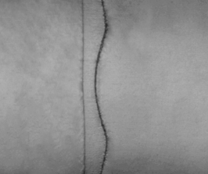
Figure 6. Typical schlieren images showing the interface evolution and wave patterns. The interface displayed is the part within 45 mm on either side of the horizontal symmetry axis of the experimental area.
Temporal variations of the perturbation amplitude  $a$ before the second impact occurs, obtained from experiments and predicted by (2.1)–(2.6), are shown in figure 7(a). The good agreement between experimental and analytical results verifies the reliability of the combined model for predicting the evolution of the once-shocked heavy–light interface. The amplitude evolution of the double-shocked interface in dimensionless form for different cases is plotted in figure 7(b), in which
  $a$ and
  $t$ are scaled as
  $\alpha =k(a-a^*)$ and
  $\tau =k |\dot {a}_2^-|(t - t^*)$, respectively, with
  $t^*$ denoting the moment when the start-up process of the double-shocked interface is completed in the experiments and
  $a^*$ being the corresponding
  $a$ at
  $t=t^*$. It is found that the combined model predicts well the amplitude evolution of the double-shocked interface under all considered conditions, and all seven manipulation possibilities have been achieved in the experiments. To sum up, RMI growth at a heavy–light interface can be effectively manipulated using successive shocks.

Figure 7. (a) Temporal variations of perturbation amplitude of once-shocked interface, where the solid line denotes theoretical prediction by (2.1)–(2.6). (b) Amplitude evolution of double-shocked interface in dimensionless form, where solid lines represent theoretical predictions by (2.1)–(2.7). Error bars represent potential errors in extracting the interface amplitude, with a length equal to half the width of the interface in the experimental schlieren image.
5. Conclusions
Manipulation of RMI growth at a heavy–light interface via successive shocks is theoretically analysed and experimentally realized. Theoretically, first, an analytical combined model is established to forecast the instability evolution before and after the second shock impact. The possibilities for the amplitude evolution pattern are then systematically discussed, and the parameter conditions for each scenario are identified. Experimentally, using a newly developed shock-tube facility and an improved soap-film technique to generate controllable successive shocks and the initial interface, respectively, all manipulation possibilities are realized by altering the time interval between two impacts.
The present work indicates that the manipulation of RMI growth through successive shocks is both achievable and predictable. This may enhance our understanding of manipulating hydrodynamic instabilities in real applications such as ICF. Notably, the current study and most available research focus on two-shock systems. In ICF, however, an implosion is generally initiated via three or more shock waves to achieve a quasi-isentropic compression of the fuel. Inspired by this, the manipulation of interface instability in a three-shock system will be explored in future work.
Acknowledgements
The authors appreciate the valuable suggestions of the reviewers.
Funding
This work was supported by the National Natural Science Foundation of China (nos 12102425, 12372281 and 12388101), the Strategic Priority Research Program of Chinese Academy of Sciences (no. XDB0620201), Youth Innovation Promotion Association CAS, the Fundamental Research Funds for the Central Universities and Young Elite Scientists Sponsorship Program by CAST (no. 2023QNRC001).
Declaration of interests
The authors report no conflict of interest.
Appendix A. Determination of nonlinear model utilized in combined model
To determine the nonlinear model utilized in the combined model, an experiment on the evolution of a single-shocked single-mode SF $_6$–air interface is performed. Note that the shock intensity is identical to that of the first shock in experiments on S-RMI presented in § 4. In addition, the initial perturbation (gas component) is identical (nearly identical) to that in S-RMI experiments. Figure 8(a) shows the schlieren images of the perturbation evolution of the once-shocked SF
 $_6$–air interface. The interface amplitude evolution extracted from the experimental images is presented in figure 8(b).

Figure 8. (a) Typical schlieren images of the evolution of a single-mode SF $_6$–air interface accelerated by a single shock. (b) The temporal variations of amplitude obtained from experiment and predicted by models: Exp, experimental results; SEA, DR and ZG, predictions from the combinations of (2.1)–(2.5) with the SEA, DR and ZG models, respectively.
Typical nonlinear models including the SEA model (Sadot et al. Reference Sadot, Erez, Alon, Oron, Levin, Erez, Ben-Dor and Shvarts1998), the DR model and the ZG model (Zhang & Guo Reference Zhang and Guo2016) are considered as candidates to comprise the combined model. The predictions from the combinations of (2.1)–(2.5) with these nonlinear models are plotted in figure 8(b). It is observed that the combined model using the DR model provides the most accurate prediction of the experimental results.
Appendix B. Comparison of models predicting double-shocked interface evolution
There are two existing models for predicting the linear evolution of the double-shocked interface: the MIK-L model (Mikaelian Reference Mikaelian1985) and the Cha-model (Charakhch'yan Reference Charakhch'yan2000, Reference Charakhch'yan2001). Here, we briefly discuss the shortcomings of these models in predicting the linear evolution of the double-shocked interface and the improvements afforded by our combined model compared with them.
The Cha-model proposed by Charakhch'yan (Reference Charakhch'yan2000, Reference Charakhch'yan2001) does not include a relation/model to predict the amplitude evolution of the once-shocked interface and relies on the pre-reshock amplitude growth rate extracted from numerical simulation or experiment. Thus, its application is highly limited. The MIK-L model proposed by Mikaelian (Reference Mikaelian1985) only describes the compression stage and the linear stage of the amplitude evolution of the once-shocked interface, without considering the start-up process and nonlinear evolution period. Therefore, the MIK-L model would be limited in accuracy for cases with reshock occurring in the linear stage and inapplicable to cases with reshock occurring at the nonlinear stage. In addition, the MIK-L model assumes that the amplitude variation rates induced by IS $_1$ and IS
 $_2$ can be calculated by the impulsive model. Thus, it is applicable only for scenarios with a light–heavy interface. In contrast to the MIK-L model, the combined model proposed in the present work comprehensively considers the amplitude variation of the once-shocked interface in the compression, start-up, linear and nonlinear stages. In addition, the WNi model (Wouchuk & Nishihara Reference Wouchuk and Nishihara1997), which applies to RMI on both light–heavy and heavy–light interfaces, is adopted to predict the amplitude variation rates induced by IS
 $_1$ and IS
 $_2$. Therefore, compared with the MIK-L model, the combined model provides a more accurate description of the pre-reshock interface evolution state, which serves as the initial condition for the second impact, and thus is capable of more accurately predicting the linear amplitude evolution of the double-shocked interface.
To examine the above analysis, a comparison of  $\dot {a}_2^+$ obtained from experiments (
 $\dot {a}_2^{+E}$) and predicted by the combined model (
 $\dot {a}_2^{+C}$) and the MIK-L model (
 $\dot {a}_2^{+M}$) is performed. The MIK-L model, which was shown to be applicable to S-RMI at a light–heavy interface (Wang et al. Reference Wang, Cao, Chen, Zhai and Luo2022), can be expressed as
 \begin{equation}
\left.\begin{array}{c@{}} \dot{a}_2^-=ka_0A_1\Delta
u_1(1-\Delta u_1/v_1^i),\\
\dot{a}_2^+=\dot{a}_2^-+k[a_0(1-\Delta
u_1/v_1^i)+\dot{a}_2^-(\Delta t-2a_0/v_1^i)]A_2 \Delta u_2
[1-\Delta u_2/(v_2^i-\Delta u_1)], \end{array}\right\}
\end{equation}
\begin{equation}
\left.\begin{array}{c@{}} \dot{a}_2^-=ka_0A_1\Delta
u_1(1-\Delta u_1/v_1^i),\\
\dot{a}_2^+=\dot{a}_2^-+k[a_0(1-\Delta
u_1/v_1^i)+\dot{a}_2^-(\Delta t-2a_0/v_1^i)]A_2 \Delta u_2
[1-\Delta u_2/(v_2^i-\Delta u_1)], \end{array}\right\}
\end{equation}
where  $A_2=(\rho _2^d-\rho _2^u)/(\rho _2^d+\rho _2^u)$ is the Atwood number of the double-shocked interface. The Cha-model is excluded from the comparison as it cannot predict the evolution of the once-shocked interface. The comparison of
  $\dot {a}_2^{+E}$,
  $\dot {a}_2^{+C}$ and
  $\dot {a}_2^{+M}$ is shown in table 2, illustrating that the combined model predicts well the experimental results and outperforms the MIK-L model.
Table 2. Comparison of the linear amplitude growth rates of double-shocked interface ( $\dot {a}_2^+$) obtained from experiments (
 $\dot {a}_2^{+E}$) and predicted by the combined model (
 $\dot {a}_2^{+C}$) and the MIK-L model (
 $\dot {a}_2^{+M}$).

Appendix C. Effects of boundary layer on shocks and interface
C.1. Shock waves
The boundary layer formed behind the first shock wave IS $_1$ will generate rarefaction waves that overtake and attenuate IS
 $_1$ (Mirels Reference Mirels1957). However, according to our previous experimental results (Wang et al. Reference Wang, Cao, Chen, Zhai and Luo2022), the boundary-layer effect on IS
 $_1$ intensity is limited. The boundary layer behind IS
 $_1$ serves as an obstacle for the propagation of the second shock IS
 $_2$, reducing its velocity. According to our previous work (Wang et al. Reference Wang, Cao, Chen, Zhai and Luo2022), the boundary layer has a more significant effect on IS
 $_2$ intensity than on IS
 $_1$ intensity. Consequently, the timing of the reshock relative to the first impact, i.e. the time interval between two shock impacts, will be prolonged with respect to the theoretical counterpart.
In addition to shock intensities and the time interval between shock impacts, the boundary layer also potentially affects the shapes of the shock waves. Although IS $_1$ is affected by rarefaction waves generated by the boundary layer, it appears to be fairly flat in the present and previous experiments (Wang et al. Reference Wang, Cao, Chen, Zhai and Luo2022). This indicates that the boundary-layer effect on the shape of IS
 $_1$ is limited. IS
 $_2$ is continuously disturbed during its propagation since the velocities of the fluids within the main flow and boundary layer differ significantly. However, a curved shock wave has the characteristic of recovering a flat shape as it moves through a tunnel with a constant cross-section (Ishizaki et al. Reference Ishizaki, Nishihara, Sakagami and Ueshima1996; Bates Reference Bates2004), i.e. the self-recovery characteristic of shock waves. As a result, the boundary-layer effect and self-recovery characteristic have an opposite influence on the perturbation at IS
 $_2$. In all present experiments, IS
 $_2$ maintains an almost flat shape under the combined influence of the boundary-layer effect and the self-recovery characteristic.
C.2. Interface
The effect of the boundary layer on interface evolution can be evaluated from the following two perspectives.
First, the boundary-layer thickness at the interface. The interface evolution is affected more heavily if the boundary layer is thicker. Since the shock waves are weak, the flow field behind them can be considered laminar and incompressible, and the boundary-layer displacement thickness at the interface ( $\delta ^*$) can be approximately calculated by the expression
  $\delta ^*=\sqrt {{{\rm \pi} }/{2}} \sqrt {2\nu _w x/u_e} ({u_w}/{u_e}-1)$ (Mirels Reference Mirels1956). Here,
  $x$ is the maximum distance between the interface and the shock during the experimental time,
  $\nu _w=\mu /\rho$, where
  $\mu$ (
 $\rho$) is the viscosity coefficient (density) of the gas, and
  $u_w$ and
  $u_e$ are the velocity of the shock and its relative velocity with respect to the interface. In our experiments, after the second shock passes through the interface,
  $x$ is
  $\sim$330 mm,
  $\mu$ of air (SF
 $_6$) is
  ${\sim }1.81\times 10^{-5}$ Pa s (
 $1.60\times 10^{-5}$ Pa s),
  $\rho$ of the gas downstream (upstream) of the double-shocked interface is 1.69 kg m
 $^{-3}$ (9.36 kg m
 $^{-3}$) and
  $u_e$ (
 $u_w$) for the double-shocked interface is 332.8 m s
 $^{-1}$ (457.9 m s
 $^{-1}$). Accordingly,
  $\delta ^*$ is calculated to be approximately 0.04 and 0.02 mm for air and SF
 $_6$, respectively. Thickness
  $\delta ^*$ is significantly smaller than the height and width of the flow cross-section (6 and 140 mm), indicating that the boundary layer has a negligible effect on the interface evolution.
Second, the interface movement and profile. The effect of the boundary layer on the interface evolution is manifested through pressure waves that introduce additional acceleration to the interface. According to figure 4, the interface movement agrees well with the 1-D theoretical results which do not consider any waves other than the two incident successive shocks. In addition, the disturbance at the initial flat interface remains limited throughout the experiment. These results indicate that the effect of the boundary layer on the interface evolution is also limited.


