


1. Introduction
The Richtmyer–Meshkov instability (RMI) (Richtmyer Reference Richtmyer1960; Meshkov Reference Meshkov1969) of shock accelerated density interfaces plays a significant role in processes as varied as inertial confinement fusion (ICF) (Lindl et al. Reference Lindl, Landen, Edwards and Moses2014; Smalyuk et al. Reference Smalyuk, Weber, Landen, Ali, Bachmann, Celliers, Dewald, Fernandez, Hammel and Hall2019) and supernovae (Arnett Reference Arnett2000). In these physical phenomena, the materials involved are in the plasma state. The RMI is most frequently modelled with the equations of hydrodynamics (Lombardini, Pullin & Meiron Reference Lombardini, Pullin and Meiron2014) or, for the plasma RMI, magnetohydrodynamics (Wheatley, Samtaney & Pullin Reference Wheatley, Samtaney and Pullin2005; Sano, Inoue & Nishihara Reference Sano, Inoue and Nishihara2013; Mostert et al. Reference Mostert, Wheatley, Samtaney and Pullin2015, Reference Mostert, Pullin, Wheatley and Samtaney2017), which are single-fluid models. These do not account for the effects of finite plasma length scales, electron inertia and a finite speed of light, which include phenomena such as charge separation and self-consistently generated electromagnetic fields. These effects may be included with an ideal two-fluid plasma model (Bellan Reference Bellan2006; Abgrall & Kumar Reference Abgrall and Kumar2014; Bond et al. Reference Bond, Wheatley, Samtaney and Pullin2017) or a reduced set of equations according to the problem at hand (Shen et al. Reference Shen, Li, Pullin, Samtaney and Wheatley2018; Li & Livescu Reference Li and Livescu2019). The importance of these effects on the evolution of the initially unmagnetised plasma RMI have been investigated for a thermal interface by Bond et al. (Reference Bond, Wheatley, Samtaney and Pullin2017) where the dynamics of the light and highly mobile electron fluid was found to play a significant role in the evolution of the RMI. A precursor electron shock creates substantial charge separation when it accelerates the electron density interface. The electron density distribution then continually overshoots that which would neutralise the plasma, resulting in an oscillatory electric field that drives oscillation of the density interfaces. This drives a secondary variable acceleration Rayleigh Taylor instability (RTI) of the interfaces, causing the electron interface to rapidly develop fine scale structures and become chaotic. The ion shock interaction produces a longer-lived region of net positive charge causing sustained electrical acceleration of the interfaces. The resulting RTI causes the low-mode growth of the ion interface to substantially exceed the single-fluid case. The transmitted ion shock is distorted due to its electromagnetic interaction with rapidly propagating electron vortices. These effects are reduced for smaller length scale plasmas, but enhanced instability is still encountered. These results imply that shock-driven instabilities may be more detrimental to ICF than predicted by single-fluid models: the increased interfacial growth rates and high-wavenumber instability seen in the two-fluid model may drive increased mixing, and the distortion of the ion shock may affect its convergence.
The influence of a magnetic field on the evolution of the RMI has been investigated previously in the context of ideal magnetohydrodynamics (MHD) (Samtaney Reference Samtaney2003; Wheatley et al. Reference Wheatley, Samtaney and Pullin2005; Sano et al. Reference Sano, Inoue and Nishihara2013; Wheatley et al. Reference Wheatley, Samtaney, Pullin and Gehre2014; Mostert et al. Reference Mostert, Wheatley, Samtaney and Pullin2015, Reference Mostert, Pullin, Wheatley and Samtaney2017) where it was found that the RMI is suppressed due to the transport of vorticity on discontinuous waves. In Hall-MHD, incompressible linear theory shows that vorticity transport is instead via a dispersive wave system, but the growth of the RMI is still mitigated (Shen et al. Reference Shen, Pullin, Wheatley and Samtaney2019). The magnetic suppression of the MHD RMI has then been investigated in the converging geometries relevant to the ICF for a variety of realisable imposed magnetic-field configurations (Mostert et al. Reference Mostert, Wheatley, Samtaney and Pullin2015, Reference Mostert, Pullin, Wheatley and Samtaney2017; Li, Samtaney & Wheatley Reference Li, Samtaney and Wheatley2018) with the goal of supressing the instabilities while minimising implosion distortion or weakening. Experimental work has also been carried out by Hohenberger et al. (Reference Hohenberger, Chang, Fiskel, Knauer, Betti, Marshall, Meyerhofer, Séguin and Petrasso2012) resulting in increased ion temperature and neutron yield and thus demonstrating the potential benefits of applied magnetic fields in ICF experiments.
Given that two-fluid effects can significantly alter the evolution of the initially unmagnetised plasma RMI (Bond et al. Reference Bond, Wheatley, Samtaney and Pullin2017), a natural question is what role they play in the magnetised plasma RMI. Of particular interest is whether the effectiveness of magnetic mitigation of the instability varies in the more realistic two-fluid plasma model. In this work, we study the canonical planar single-mode RMI with an initial magnetic field that is normal to the interface location using ideal two-fluid plasma simulations. We perform our investigation over a range of plasma length scales such that we demonstrate ion–electron plasmas with a range of coupling strengths between the species. We also compare with solutions from unmagnetised plasma flows and comparable hydrodynamic flows. We begin in § 2 by describing the two-fluid plasma model that is implemented in our simulation software. In § 3 we give an outline of the initial conditions for the various simulations. Results and discussion are then presented in § 4, followed by some concluding remarks in § 5.
2. The two-fluid plasma model
The two-fluid Euler equations for the ions and electrons with appropriate electromagnetic forcing terms are,
 \begin{gather} \frac{\partial\rho_{\alpha}}{\partial t}+\boldsymbol{\nabla} \boldsymbol{\cdot}(\rho_{\alpha}\boldsymbol{u}_{\alpha})= 0, \end{gather}
 \begin{gather}\frac{\partial\rho_\alpha\boldsymbol{u}_\alpha}{\partial t}+\boldsymbol{\nabla} \boldsymbol{\cdot}(\rho_{\alpha}\boldsymbol{u}_{\alpha} \boldsymbol{u}_{\alpha}+p_{\alpha}{\boldsymbol{\mathsf{I}})= n_{\alpha}q_{\alpha}(\boldsymbol{E}+\boldsymbol{u}_{\alpha}\times\boldsymbol{B}),} \end{gather}
 \begin{gather}\frac{\partial\epsilon_{\alpha}}{\partial t}+\boldsymbol{\nabla} \boldsymbol{\cdot}((\epsilon_{\alpha}+p_{\alpha})\boldsymbol{u}_{\alpha})= n_{\alpha}q_{\alpha}\boldsymbol{u}_{\alpha}\boldsymbol{\cdot}\boldsymbol{E}, \end{gather}
where
 \begin{equation} \rho_{\alpha}= n_{\alpha}m_{\alpha}, \quad p_{\alpha}= n_{\alpha}k_{B}T_{\alpha}, \quad \epsilon_{\alpha}= \frac{p_{\alpha}}{\gamma_\alpha-1}+\frac{\rho_{\alpha}| \boldsymbol{u}_{\alpha}|^{2}}{2}. \end{equation}
Here,  $\alpha$ gives the species with
  $\rho _{\alpha }$ the species density,
  $n_\alpha$ the number density,
  $m_\alpha$ the particle mass,
  $p_\alpha$ the pressure and
  $T_\alpha$ the temperature, with
  $k_B$ the Boltzmann constant. The species energy
  $\epsilon _\alpha$, has contributions from velocity
  $\boldsymbol {u}_{\alpha }=(u_{\alpha },\ v_{\alpha },\ w_{\alpha })^\textrm {T}$ and pressure
  $p_\alpha$ with the ratio of specific heats
  $\gamma _\alpha$. The ratio of particle charge
  $q_\alpha$ to mass is given by
  $r_{\alpha }={q_{\alpha }}/{m_{\alpha }}$. Each species is in its own kinetic-collisional equilibrium but without inter-species collisions. The species interact via the induced electric,
  $\boldsymbol {E}$, and magnetic,
  $\boldsymbol {B}$, fields according to Maxwell's equations with correction potentials for divergence constraints according to (Munz, Schneider & Voss Reference Munz, Schneider and Voss2000b),
 \begin{gather} \frac{\partial\boldsymbol{B}}{\partial t}+\boldsymbol{\nabla}\times\boldsymbol{E}+\varGamma_{B}\boldsymbol{\nabla}\psi_{B}= 0, \end{gather}
 \begin{gather}\frac{\partial\boldsymbol{E}}{\partial t}-c^{2}\boldsymbol{\nabla}\times\boldsymbol{B}+c^{2}\varGamma_{E}\boldsymbol{\nabla}\psi_{E}= -\frac{\boldsymbol{j}}{\epsilon_{0}}, \end{gather}
 \begin{gather}\frac{\partial\psi_{E}}{\partial t}+\varGamma_{E}\boldsymbol{\nabla} \boldsymbol{\cdot}\boldsymbol{E}= \frac{\varGamma_{E}}{\epsilon_{0}}\rho_{c}, \end{gather}
 \begin{gather}\frac{\partial\psi_{B}}{\partial t}+c^{2}\varGamma_{B}\boldsymbol{\nabla} \boldsymbol{\cdot}\boldsymbol{B}= 0, \end{gather}
where the charge density  $\varrho _{c}$ and current density
  $\boldsymbol {j}$ are given as sums over the plasma species
  $\alpha$ according to,
 \begin{equation} \rho_{c} =\sum_{\alpha}\frac{q_{\alpha}}{m_{\alpha}}\rho_{\alpha}, \quad \boldsymbol{j} =\sum_{\alpha}\frac{q_{\alpha}}{m_{\alpha}}\rho_{\alpha}\boldsymbol{u}_{\alpha}. \end{equation}
 In these equations we have the speed of light  $c$, given by
  $c^{2}={1}/{\mu _{0}\epsilon _{0}}$ with permeability of free space
  $\mu _{0}$ and vacuum permittivity
  $\epsilon _{0}$. The correction potentials
  $\psi$ and the associated wave speeds
  $\varGamma$ serve to enforce the divergence constraints. Non-dimensionalisation of these sets of equations is carried out according to the following,
 \begin{gather} \hat{n}= \frac{n}{n_{0}}, \quad \hat{m}= \frac{m}{m_{0}}, \quad \hat{q}= \frac{q}{q_{0}}, \quad \hat{\rho}= \frac{\rho}{\rho_{0}}, \end{gather}
 \begin{gather}\hat{\boldsymbol{u}}= \frac{\boldsymbol{u}}{u_{0}}, \quad \hat{p}= \frac{p}{n_{0}m_{0}u_{0}^{2}} \quad \hat{\epsilon}= \frac{\epsilon}{n_{0}m_{0}u_{0}^{2}}, \quad \hat{x}= \frac{x}{L_0}, \end{gather}
 \begin{gather}\hat{c}= \frac{c}{u_{0}}, \quad \hat{t}= \frac{t}{t_{0}}, \quad \hat{\boldsymbol{B}}= \frac{\boldsymbol{B}}{B_{0}}, \quad \hat{\boldsymbol{E}}= \frac{\boldsymbol{E}}{cB_{0}}, \end{gather}
 \begin{gather}\hat{\psi}_{E}= \frac{\psi_{E}}{B_{0}}, \quad \hat{\psi}_{B}= \frac{\psi_{B}}{cB_{0}}, \quad \hat{d}_{S}= \frac{d_{S,0}}{L_0}, \end{gather}
where we have reference quantities for length  $L_0$, number density
  $n_0$, mass
  $m_0$, temperature
  $T_0$, magnetic field
  $B_0$ and velocity
  $u_0=\sqrt {{k_B T_0}/{m_0}}$, from which we then have reference time according to
  $t_0={L_0}/{u_0}$. The reference plasma skin depth
  $d_{S,0}$, and magnetic interaction parameter
  $\beta _{0}$, along with the conversion to Debye length and Larmor radius, are given according to (Shen et al. Reference Shen, Li, Pullin, Samtaney and Wheatley2018),
 \begin{gather} d_{S,0}\equiv \frac{1}{q_{0}}\sqrt{\frac{m_{0}}{\mu_{0}n_{0}}}, \quad \beta_{0} \equiv \frac{2\mu_{0}n_{0}m_{0}u_{0}^{2}}{B_{0}^{2}}, \end{gather}
 \begin{gather}d_{D,0}= \frac{d_{S,0}}{c}, \quad d_{L,0}= \sqrt{\frac{\beta_0}{2}}d_{S,0}. \end{gather}
A local value for the magnetic interaction can be calculated according to  $\beta ={\beta _{0}\hat {p}}/{\hat {B}^{2}}$ where it is noted that the combined pressure,
  $\hat {p}=\hat {p}_i + \hat {p}_e$, is used. From this point on we will dispense with the caret notation and assume that all quantities are dimensionless unless otherwise specified. Non-dimensional evolution equations for the fields are then given by,
 \begin{gather} \frac{\partial\boldsymbol{B}}{\partial t}+c\boldsymbol{\nabla}\times\boldsymbol{E} +c\varGamma_{B}\boldsymbol{\nabla}\psi_{B}= 0, \end{gather}
 \begin{gather}\frac{\partial\boldsymbol{E}}{\partial t}-c\boldsymbol{\nabla}\times\boldsymbol{B} +c\varGamma_{E}\boldsymbol{\nabla}\psi_{E}= -\frac{c}{d_{S,0}} \sqrt{\frac{\beta_{0}}{2}}\boldsymbol{j}, \end{gather}
 \begin{gather}\frac{\partial\psi_{E}}{\partial t}+c\varGamma_{E}\boldsymbol{\nabla} \boldsymbol{\cdot}\boldsymbol{E} =\frac{c^{2}\varGamma_{E}}{d_{S,0}} \sqrt{\frac{\beta_{0}}{2}}\varrho_{c}, \end{gather}
 \begin{gather}\frac{\partial\psi_{B}}{\partial t}+c\varGamma_{B}\boldsymbol{\nabla} \boldsymbol{\cdot}\boldsymbol{B}= 0, \end{gather}
and for the plasma components,
 \begin{gather} \frac{\partial\rho_{\alpha}}{\partial t}+\boldsymbol{\nabla} \boldsymbol{\cdot}(\rho_{\alpha}\boldsymbol{u}_{\alpha})= 0, \end{gather}
 \begin{gather}\frac{\partial\rho_{\alpha}\boldsymbol{u}_{\alpha}}{\partial t}+\boldsymbol{\nabla} \boldsymbol{\cdot}(\rho_{\alpha}\boldsymbol{u}_{\alpha}\boldsymbol{u}_{\alpha}+ p_{\alpha}{\boldsymbol{\mathsf{I}})= \phi_{\alpha}\rho_{\alpha}(c\boldsymbol{E}+\boldsymbol{u}_{\alpha} \times\boldsymbol{B}),} \end{gather}
 \begin{gather}\frac{\partial\epsilon_{\alpha}}{\partial t}+\boldsymbol{\nabla} \boldsymbol{\cdot}((\epsilon_{\alpha}+p_{\alpha})\boldsymbol{u}_{\alpha})= \phi_{\alpha}\rho_{\alpha}c\boldsymbol{u}_{\alpha}\boldsymbol{\cdot}\boldsymbol{E}, \end{gather}
where
 \begin{equation} \phi_{\alpha}= \sqrt{\frac{2}{\beta_{0}}}\frac{r_{\alpha}}{d_{S,0}}, \end{equation}
and  ${\boldsymbol{\mathsf{I}}}$ is a tensor with elements
  $I_{ij}=\delta _{ij}$. We also give the vorticity evolution equation,
 \begin{align} \frac{\partial\boldsymbol{\omega}_{\alpha}}{\partial t}&=\underbrace{(\boldsymbol{\omega}_{\alpha} \boldsymbol{\cdot}\boldsymbol{\nabla})\boldsymbol{u}_{\alpha}}_{\tau_{v}}- \underbrace{(\boldsymbol{u}_{\alpha}\boldsymbol{\cdot}\boldsymbol{\nabla}) \boldsymbol{\omega}_{\alpha}}_{\tau_{c}}-\underbrace{\boldsymbol{\omega}_{\alpha}(\boldsymbol{\nabla} \boldsymbol{\cdot}\boldsymbol{u}_{\alpha})}_{\tau_{s}}\nonumber\\ &\quad +\underbrace{\frac{1}{\rho_{\alpha}^{2}}(\boldsymbol{\nabla}\rho_{\alpha} \times\boldsymbol{\nabla} p_{\alpha})}_{\tau_{b}}+\underbrace{\phi_{\alpha}c (\boldsymbol{\nabla}\times\boldsymbol{E})}_{\tau_{E}}+\underbrace{\phi_{\alpha} (\boldsymbol{\nabla}\times(\boldsymbol{u}_{\alpha}\times\boldsymbol{B}) )}_{\tau_{B}}, \end{align}
where  $\tau _v$ and
  $\tau _s$ are the stretching of vorticity due to velocity and compressibility,
  $\tau _c$ is the convective transport of vorticity,
  $\tau _{b}$ is the baroclinic torque and
  $\tau _E$ and
  $\tau _B$ are the torque from electric and magnetic contributions to the Lorentz force.
2.1. Numerical implementation
Numerical solutions are obtained in one and two space dimensions with three components for all vector quantities. For two-dimensional flows we thus have  ${\partial }/{\partial z} = 0$ while
  $w\neq 0$,
  $B_z\neq 0$,
  $E_z\neq 0$, and likewise for all derived vector quantities. The solver is implemented within the adaptive mesh refinement (AMR) framework AMReX (Zhang et al. Reference Zhang, Almgren, Beckner, Bell, Blaschke, Chan, Day, Friesen, Gott and Graves2019) and consists of a finite-volume scheme with a two-stage, second-order Runge–Kutta time integrator (Gottlieb, Shu & Tadmor Reference Gottlieb, Shu and Tadmor2001) with minmod limited interface values for flux calculation (Abgrall & Kumar Reference Abgrall and Kumar2014). Fluxes are calculated at cell interfaces via the HLLE (Harten–Lax–van Leer–Einfeldt) (Einfeldt Reference Einfeldt1988) approximate Riemann solver. The HLLE scheme for Maxwell's equations uses the speed of light as the maximum wave speed while for the species equations the hydrodynamic sound speed is used. Contributions from source terms are solved locally with the implicit method of Abgrall & Kumar (Reference Abgrall and Kumar2014) allowing a time step restriction based entirely on the wave speeds present in the domain. To approximately satisfy the divergence constraints of Maxwell's equations a Lagrange multiplier method is used, according to (2.16) through (2.19), that mitigate divergence errors without requiring the solution of Poisson equations (Munz, Ommes & Schneider Reference Munz, Ommes and Schneider2000a). Mesh refinement is performed when the ion or electron density gradient exceeds 0.1 in any direction according to,
 \begin{equation} \varepsilon=\frac{\rho_{1}-2\rho_{0}+ \rho_{-1}}{ |\rho_{1}-\rho_{0} |+ |\rho_{0}-\rho_{-1} |+0.01 (\rho_{1}+2\rho_{0}+\rho_{-1} )}, \end{equation}
where the subscript indicates relative cell index in any of the spatial coordinates. Verification of this solver has been performed against the test cases used in Bond et al. (Reference Bond, Wheatley, Samtaney and Pullin2017) with closely similar results and thus will not be presented here.
3. Simulation outline
Initial conditions for the RMI in two-dimensional (2-D)  $(x-y)$ space consist of a three-zone Riemann problem in the
  $y$-periodic domain
  $(-50 \le x \le 50,\,0 \le y \le 1)$. The
  $x$-boundary is defined with zero gradient for all quantities. Note that the domain is large enough in the
  $x$ direction that no reflected waves are able to interfere with the flow about the interface. A schematic of the domain can be seen in figure 1. The three zones are denoted
  $S_{0}$,
  $S_{1}$ and
  $S_{2}$ with planar left interface
  $I_{L}$ separating
  $S_{0}$ and
  $S_{1}$ and a sinusoidally perturbed right interface
  $I_{R}$ separating
  $S_{1}$ and
  $S_{2}$. The left and right interfaces initialise a shock and density interface respectively. A single perturbation wavelength spans the domain with an amplitude of
  $0.1$, which is
  $\frac {1}{10}$ of the domain width.
  $I_{L}$ is separated from the mean location of
  $I_{R}$ by a distance of 0.2. Interface
  $I_{R}$ is defined by a hyperbolic tangent profile, aligned with
  $x$, according to
 \begin{equation} f(x)=f_{R}+\frac{f_{L}-f_{R}}{2}\left(1+\tanh\left(\frac{2x}{\eta_w}\mathrm{arctanh} \left(\frac{9f_{R}-10f_{L}}{10\left(\,f_{L}-f_{R}\right)}\right)\right)\right), \end{equation}
where  $f_{L}$ and
  $f_{R}$ give the left and right values and
  $\eta _w=0.01$ is the width containing 90 % of the variation across the interface. Outside of interface
  $I_{R}$ the states are uniform with initial conditions given in table 1 resulting in a normal shock with Mach number of
  $M_{s}=2$ in the ion fluid impacting a perturbed interface with a density ratio of 3. The divergence correction potentials wave speed is defined with
  $\varGamma =1$ while a CFL (Courant–Friedrichs–Lewy) condition of 0.3 is used for all cases based on the maximum wave speed in the domain, the speed of light. Table 1 defines four overall cases, a magnetised thermal RMI (MTRMI) case, which provides the primary results presented in this work, un-magnetised thermal RMI (TRMI) and hydrodynamic cases. Each of these will now be described in greater detail.

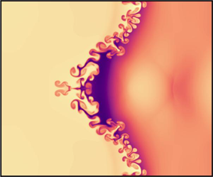
Figure 1. Initial conditions for  $d_{S,0}=10$ and
  $\beta =0.1$ with contour levels showing normalised gradient of electron number density at initial and final time.
Table 1. Simulation initial conditions outline.

3.1. Magnetised thermal RMI
The MTRMI case is defined as a thermal RMI with initial magnetic field normal to the density interface. The electron state is identical to that of the ions except for the density which is defined according to  $\rho _{e}=({m_{e}}/{m_{i}})\rho _{i}$ such that charge density is initially zero at all points in the domain. As shown in table 1 the ion to electron mass ratio is set to 100, with
  $m_{i}=1$ and
  $m_{e}=0.01$ while
  $m_0 = 9.11\times 10^{-29}$ kg (100 times the dimensional electron mass). This mass ratio is lower than the physical value of 1836 for a hydrogen plasma, and thus reduces the problem stiffness, but is large enough to ensure that the electron dynamics is relatively fast. The ion and electron charges are
  $q_{i}=1$ and
  $q_{e}=-1$. A range of plasma regimes are considered, with
  $0.1 \leq d_{S,0} \leq 10$ and
  $0.1 \leq \beta \leq 1$ with
  $\beta _0=1$, along with a non-dimensional speed of light
  $c=50$. This value of
  $c$ implies a reference temperature of the order of the hot spot temperature in a ICF capsule implosion (
 $T=5\times 10^{3}$ eV Srinivasan & Tang Reference Srinivasan and Tang2012). Despite this temperature being at the limit of practical interest, it is used to make the problem more computationally tractable by reducing the separation of scales between the wave speeds. Such an approach is common in two-fluid plasma simulations (e.g. Loverich, Hakim & Shumlak Reference Loverich, Hakim and Shumlak2011; Bond et al. Reference Bond, Wheatley, Samtaney and Pullin2017). The AMR configuration and effective resolution required is dependent on the plasma regime being simulated and is thus discussed further in the Appendix.
3.2. Un-magnetised thermal RMI
In order to further understand the results computed for the MTRMI conditions we also solve cases with an initial magnetic field of zero. These solutions correspond closely to those generated by Bond et al. (Reference Bond, Wheatley, Samtaney and Pullin2017) with small variation in the plasma parameters according to (2.14a,b) and (2.15a,b). This case illustrates the flow with both electric and magnetic fields being generated due to the motion of charged fluids without any initial field being defined.
3.3. Hydrodynamic thermal RMI
Reference solutions are also computed for hydrodynamic RMI such that baseline solutions may be compared across the full range of plasma parameters. Two solutions were chosen to act as references that correspond to the two limits of plasma skin depth i.e.  $d_{S,0} = 0$ and
  $d_{S,0}\rightarrow \infty$. These two limits can be mapped to solutions of the hydrodynamic RMI in the following manner. Firstly,
  $d_{S,0}\rightarrow \infty$ gives zero coupling between the species within the plasma as there is no interaction with the electromagnetic fields, this can be seen in (2.21) and (2.22) where the source terms go to zero. Thus we are left with the hydrodynamic evolution equations and, as we are primarily interested in the ion fluid evolution, we may simply perform a simulation based on the ion component of the two-fluid problem specification supplied above with
  $q_i=0$. This gives us a classic RMI problem with fluid pressure in region
  $S_1$ of
  $p=0.5$, corresponding to the partial pressure of the ion species. This pressure is important to note as the other limiting case, where
  $d_{S,0}=0$, has a pressure of
  $p=1$. This is because for
  $d_{S,0}=0$ the ion and electron fluids are tightly coupled and, assuming zero relative velocity, behave as essentially a single neutral fluid. This condition can thus be approximated by having a single neutral fluid with total pressure according to
  $p=p_i + p_e=1$. We thus have our two reference hydrodynamic solutions that map to the case of infinite plasma length scale for
  $p=0.5$ and zero plasma length scale with
  $p=1$. Maintaining an initial shock Mach number of 2 for the
  $p=1$ case then requires modification of the initial pressure jump conditions as shown in table 1. We will henceforth refer to these two solutions by the corresponding pressure.
4. Results
The evolution of the ion and electron number densities are shown in figure 2 for skin depths of  $0.1 \leq d_{S,0} \leq 10$, magnetic interaction parameter of
  $\beta =0.1$ and for a time span of
  $0.05 \leq t \leq 1$. The electron and ion fluids are shown in the upper and lower half of each frame, respectively. We begin by discussing the evolution of the
  $d_{S,0}=10$ case (corresponding to a Debye length of
  $d_{D,0}=d_{S,0}/c=0.2$) where coupling between the ions and electrons is low as a result of the large plasma length scale, effectively 10 times the domain width. This loose coupling is apparent at
  $t=0.05$ where, owing to the order of magnitude greater sound speed in the electron fluid, the electron shock has completely processed the perturbed interface before the ion shock has even made contact with the interface. As discussed by Bond et al. (Reference Bond, Wheatley, Samtaney and Pullin2017), the relative motion between the discontinuities in each fluid produces bands of non-zero charge density, which in turn generate electric fields. As a consequence of these fields, by
  $t=0.1$ the electron shock has begun to weaken and the electron interface displays high wavenumber electrically driven Rayleigh–Taylor (RT) instability, which will be investigated in more detail in § 4.1. In addition, the shear deposited on the interface by the shock interaction is subject to Kelvin–Helmholtz (KH) instability. The contribution of these secondary instabilities to high-wavenumber perturbation growth varies along the interface as it will be shown subsequently that the drivers of these instabilities, the acceleration field and the interfacial shear, are non-uniform.

Figure 2. Evolution of ion and electron fluids for the magnetised thermal RMI with  $0.1 \leq d_{S,0} \leq 10$ and
  $\beta =0.1$. Each frame shows the electron (upper) and ion (lower) number density.
For the electron interface at  $t=0.1$, emergent high-wavenumber secondary instability is observed at a mean wavenumber of
  $\bar {k}\approx 45$ (see table 2). This wavenumber varies along the interface (and with time) due to the non-uniform stretching of the interface by the primary RMI mode, along with the aforementioned non-uniformity of the acceleration field and interfacial shear, thus a mean and variance for the dominant secondary instability wavenumber are provided in table 2. To the best of our knowledge, dispersion relations for the magnetised, two-fluid plasma RTI and KHI have yet to be obtained, placing a theoretical examination of the local most-unstable wavenumber beyond the scope of the present work. The primary driver for the dominant wavenumber, whether KH or RT, is thus unknown at this time.
Table 2. Dominant wavenumber of secondary interface perturbations for  $\beta =0.1$ on the ion and electron interfaces over the upper half of the domain,
  $0.5 \leq y \leq 1$. Values recorded for
  $0.02 \leq t \leq 0.1$ on different portions of the interface in order to capture mode statistics as soon as they become discernible, but before going nonlinear.

At  $t=0.2$ the ion shock has completed traversal of the interface while the electron interface is displaying significant disruption and overall growth as a result of prominent secondary instabilities along the entire interface. The flow structures arising from the secondary instabilities are aligned approximately parallel with the initial magnetic field, although at this plasma length scale there is still significant transverse motion. By this time the electron shock has completely transitioned to an oscillatory wave packet with the dispersive nature of the waves evident in the break up of the initial concentrated shock front. The ion fluid is also displaying a clear increase in density ahead of the ion shock owing to the influence of the electron fluid via the electromagnetic fields. These ion fluid disturbances seed the ion interface with perturbations which leads to discernible distortions with
  $\bar {k}\approx 18$ by
  $t=0.3$ which subsequently form KH rollers. By
  $t=0.5$ the electron interface is well mixed with significant jetting in both directions about the interface. These electron jets continue to be constrained to lie along the magnetic field which is only slightly perturbed from the initial
  $x$-alignment by the self generated fields. The RMI continues to develop in both ions and electrons and by
  $t=1$ significant KH instability has developed across the width of the ion interface while the electron interface is well mixed with significant jetting ahead of the ion shock.
For  $d_{S,0}=1$ (
 $d_{D,0}=0.02$) the increase in coupling strength between the two charged fluids is apparent at
  $t=0.05$ with the electron interface maintaining approximately the same location as the ion interface. The coupling is not strong enough, however, to prevent high speed waves generated by the initial Riemann problem from traversing the interface ahead of the ion shock. This initial wave breaks down into a wave packet more rapidly than in the
  $d_{S,0}=10$ case with the dispersive nature of the flow being apparent by
  $t=0.05$. These precursor waves in the electron fluid drive secondary instability of the ion and electron interfaces at
  $\bar {k}\approx 77$ for the ions and
  $\bar {k}\approx 65$ for the electrons. These perturbations exhibit significant variation across the interface with
  $\sigma \approx {\bar {k}}/{3.5}$. Note that, in order to quantify perturbations on the electron interface, measurements are made over a range of times corresponding with shock traversal, this is done so that measurements are taken after the shock traversal but before the secondary instability becomes nonlinear. This can be seen at
  $t=0.1$ where the electron interface has developed significant nonlinear instability downstream of the ion shock whilst upstream the interface is perturbed but not yet nonlinear. The coupling between the light and heavy fluids can again be seen at
  $t=0.1$ where the ion fluid now displays a higher density band on the upstream side of the interface ahead of the ion shock, this band perturbs the flow and enhances the destabilisation of the shock as it processes this region. This contributes to the multiple shock fronts and resulting mixing that is observed for both fluids within the region bounded by the interface and the ion shock. Jetting of the electron fluid (explored in more detail in § 4.2) is observed once again with up and downstream travelling jets from the spike and bubble portions of the interface respectively. As expected these jets are more tightly constrained by the magnetic field, relative to the
  $d_{S,0}=10$ case, as well as having reduced entrained mass. By
  $t=1$ the ion and electron interface display features of similar extent and magnitude although the electron interface is somewhat more diffuse owing to the higher mobility of that fluid. The electron jets extend from the interface in both directions by over an initial perturbation width and are aligned with the magnetic field.
Decreasing the plasma length scale by another order of magnitude to  $d_{S,0}=0.1$ (
 $d_{D,0}=0.002$) results in the ion and electron shocks being essentially locked together, on the scale of the interface perturbation, leading to approximately simultaneous excitation of the RMI in both fluids. The ion and electron fluids are shown to be tightly coupled with almost identical fluid structure shared between the two fluids. The jetting that has been observed for larger plasma length scales is now absent. The interface is seen to maintain integrity and by final time has decreased in perturbation amplitude. The transmitted shock also maintains the initial distortion imparted by processing the perturbed interface without the oscillation seen for larger values of
  $d_{S,0}$. Bands of density variation may also be observed downstream of the shock which correspond to vorticity transport that will be discussed in § 4.3.
In figure 3 we compare un-magnetised (TRMI), magnetised (MTRMI) and pure hydrodynamic flow simulations. The MTRMI and TRMI results are shown in the top and bottom half of each frame, respectively (except for the far right frames, which display hydrodynamic results). Interface locations from the  $p=0.5$ and
  $p=1$ hydrodynamic cases are given by the left and right dashed white lines, respectively. In this figure we firstly observe the significant impact that the presence of a electromagnetically coupled light and highly mobile fluid, the electrons, can have on the evolution of a heavier fluid. This is shown by the significant variation between the neutral fluid cases, where no coupling exists, and either the TRMI or MTRMI cases. Decreasing
  $d_{S,0}$ does drive the TRMI plasma solution towards the hydrodynamic solution but there is still significant local instability along the interface and growth of the primary mode. Introducing an initial magnetic field substantially reduces the instability with general unconstrained motion of the light fluid transformed into field aligned features that appear to have less of a destabilising influence on the heavier fluid. The overall growth of the magnetised RMI is seen to reduce for all plasma length scales, relative to the initially unmagnetised case, and it is this suppression of the RMI that will be investigated and quantified in later sections. This suppression is particularly evident when comparing to the reference hydrodynamic cases for
  $d_{S,0}=0.1$, where the initially unmagnetised interface is observed to have growth its primary perturbation mode that lies between the
  $p=0.5$ and the
  $p=1$ hydrodynamic cases, whereas the magnetised interface exhibits significantly lower perturbation growth than any other case. For now, however, we look in more detail at the dynamics owing to charge separation as well as the significant effect of the initial magnetic field on the electron flow.

Figure 3. Ion and electron number densities at  $t=0.75$ with zero initial magnetic field (lower half of frames) and non-zero initial magnetic field (upper half of frames). Purely hydrodynamic solutions are shown for comparison in the far right frames. Interface contours for the
  $p=\frac {1}{2}$ and
  $p=1$ cases are overlaid on all frames for reference.
4.1. Rayleigh–Taylor instability
The low inertia of the electron fluid gives it significantly enhanced mobility compared to that of the ions. For large plasma length scales this can lead to significant disparities in ion and electron flow structure (see figure 2) with non-zero charge density as a result. These regions of charge are non-stationary and thus electrical currents are generated, along with the associated electromagnetic fields. The most significant charge separation in the present work occurs due to the initial shock impacting the interface and driving differential motion in the ion and electron fluids. This can be seen in figure 4 where both magnetised and unmagnetised cases are shown for  $d_{S,0}=10$. This plasma length scale is shown to allow for easier visualisation of the effect of charge separation thanks to the exaggerated nature of phenomenon, the effects discussed in this section are also present in the smaller plasma length scale cases but are not so visually apparent. As shown in figure 4, the Riemann problem that generates the ion shock also generates an electron shock with a much higher wave speed. The different times at which the respective interfaces are then processed leads to significant differential motion and thus wide bands of charge separation with alternating sign. This leads to widespread currents, electric field generation, and bulk acceleration of the flow field. All of this can be seen in sequence in figure 4.

Figure 4. Evolution of the electron fluid produced by charge separation with  $d_{S,0}=10$. Frames show results for zero initial magnetic field (lower half) and non-zero initial magnetic field (upper half). Interface contours for ions (solid) and electrons (dashed) are also shown for reference.
The differential motion of the ion and electron shocks can be seen in the plot of  $\varrho _c$ at
  $t=0.015$ with regions of positive, negative and neutral charge density. The ion shock is also seen as the centre of a negative
  $x$-current slab which in turn generates a positive
  $x$-electric field and thus negative
  $x$-acceleration of the negatively charged electron fluid. This negative current density in
  $x$ is an indication of how the electromagnetic aspects of the flow are dominated by the fast electron dynamics. As the electron shock processes the electron interface, the interface is compressed and begins to move to the right, while the ion fluid is uncompressed and relatively stationary. This leads to a region of negative charge between the transmitted electron shock and the electron interface, since the electron number density has been shock compressed, and a region of positive net charge between the ion and electron interfaces where the low density fluid to the left of the electron interface overlaps with the high density fluid to the right of the undisturbed ion interface. These regions widen with shock progress to eventually cover the entire width of the domain. This positively charged region disrupts the acceleration field and begins to introduce the oscillations that we observe in figure 5 where the acceleration acting on the ion and electron fluid at the location of a number of massless tracer particles is shown. By
  $t=0.075$, the consistent acceleration of the electrons downstream of the transmitted electron shock in the negative
  $x$ direction has reversed their flow, as indicated by the large regions of positive
  $j_x$. The head of the electron spike now extends upstream past the ion spike resulting in a large region of negative charge density. At this point the
  $x$-electric field is multi-signed with significant variation along both ion and electron interfaces leading to the variation in acceleration seen in figure 5. As time progresses, regions of charge density continue to change sign leading to further oscillation in the acceleration field.

Figure 5. Acceleration in  $x$ of the electron (a) and ion (b) fluids generated by the electric field with
  $d_{S,0}=10$,
  $\beta =0.1$ and
  $0 \leq t \leq 0.15$. Sampled in time along the trajectory of massless tracer particles with colour scale according to particle starting
  $0 \leq y_0 \leq 1$ position. Tracer trajectories shown in the right frames with background contours of normalised number density
  $0 \leq \hat {n} \leq 1$ at
  $t=0.15$.
Due to the differential motion of the electron and ion fluids we now have an adverse acceleration field acting on the interface density gradient thus leading to the initiation of electrically driven, variable acceleration Rayleigh–Taylor instability. Owing to the universal nature of the electric field, RT instability is experienced not only by the electrons, which is clear from the evolution of the electron density field in figures 2 and 4, but also by the ion fluid. However, for the ions, the acceleration at early time is predominantly in the positive direction and is thus aligned with the density gradient. It is only at a later time that the sign of the acceleration is reversed and it is the head of the spike where this first occurs, as seen at  $t=0.125$ and 0.15 in figure 4, leading to the accelerated destabilisation of the ion interface relative to the purely hydrodynamic cases shown in figure 3. Bond et al. (Reference Bond, Wheatley, Samtaney and Pullin2017) illustrated that the band of positive net charge seen forming between the ion transmitted shock and interface at
  $t=0.15$ is persistent and leads to a negative acceleration of the ion interface in the RT unstable direction for the remainder of the simulation time, leading to enhanced growth of the primary mode relative to the hydrodynamic cases.
In figure 4 we show both the magnetised and un-magnetised cases in order to demonstrate the effect of this initial magnetic field on the driver of the RT instability (the acceleration field). From this figure we can see that while the magnitude of various properties of the flow are indeed affected, the overall nature of the acceleration remains essentially unchanged. This indicates that the observed mitigation of interfacial instability through the application of an initial magnetic field is not due to a major change in the acceleration field that drives the secondary RT instability, but rather some other effect. We thus proceed to investigate further interesting features of the flow.
4.2. Electron jet behaviour with varying  $\beta$

A striking feature of the electron flow is the field-aligned jetting of the electron fluid over large distances observed for an initial magnetic field of  $\beta = 0.1$. In order to investigate the effect of the magnetic field on this phenomenon a study was carried out for
  $d_{S,0}=10$ and
  $0.1 \leq \beta \leq \infty$ as shown in figure 6. At early time the influence of decreasing
  $\beta$, giving increased effectiveness of the magnetic field, is only visually significant for
  $\beta =0.1$ with higher wavenumber features being generated which are predominantly field aligned. The KH roller like features observed for large
  $\beta$ are transformed into mushroom like structures with stems aligned with the field. Where the slope of the interface is low, mushroom like structures are present for all
  $\beta$ and it can seen that the lateral growth of the head is also somewhat suppressed for
  $\beta =0.1$. At later time, flows having large
  $\beta$ develop large scale features which extend over a significant area, while for small
  $\beta$ the interface remains much more compact. By
  $t=0.45$ the electron interface has become highly mixed for
  $\beta >0.1$ while for
  $\beta =0.1$ the initial interface remains discernible with field aligned jets extending from the interface in both upstream and downstream directions.

Figure 6. Electron dynamics with varying  $\beta$ (hydrodynamic
  $\beta =\infty$, magnetised with loose coupling
  $\beta =1$, magnetised with strong coupling
  $\beta =0.1$) and
  $d_{S,0}=10$ for
  $0.15 \leq t \leq 0.45$ in a reference frame moving with the interface.
This jetting behaviour is attributed to the focusing of the high-wavenumber secondary instabilities, both the electrically driven RT and KH, by the action of the Lorentz force enabled by the imposed magnetic field, as shown in figure 7. In this figure acceleration of the electron fluid in the  $y$ direction owing to the magnetic component of the Lorentz force
  $a_y^{\boldsymbol {B}}=\phi \rho (\boldsymbol {u}\times \boldsymbol {B})$ (see (2.21)), is shown in the vicinity of electron jets at a time of
  $t=0.1$. Each jet is thus shown to be approximately bounded by regions of positive and negative
  $a_y^{\boldsymbol {B}}$ with the overall trajectory of the jet following the zero contour provided by this acceleration field. The Lorentz force therefore acts to compress each jet towards its axis, resisting the growth of shear instabilities on the jet boundaries that would otherwise act to transport its momentum and limit how far it is able to penetrate into the fluid surrounding the interface.

Figure 7. Magnetic-field-induced  $y$-acceleration of the electron fluid. Contour shows electron interface. Results at
  $t=0.1$ with
  $d_{S,0}=1$ and
  $\beta =0.1$. Inset indicates the region shown by the main frame.
4.3. Vorticity dynamics
From figures 2 and 3 we note the reduction in overall growth of the initial perturbed density interface as  $d_{S,0}$ decreases. In order to characterise the overall width
  $\eta$ of the interface we calculate a one-dimensional function from our volume-of-fluid tracer
  $\varphi$ and define the interface width according to,
 \begin{gather} \theta (x) = \int_0^{1}\varphi(x,y) \, \mathrm{d} y, \quad \theta (x_0) = 0.05, \end{gather}
 \begin{gather}\eta = x_1 - x_0, \quad \theta (x_1) = 0.95, \end{gather}
where  $0 \leq \varphi \leq 1$. The resulting interface width over the time of simulation is shown in the uppermost row of figure 8 along with the growth rates in the following row. Here, we are primarily interested in the ion interface as it is within this portion of the flow that the vast majority of the mass is held. In these plots we also show the corresponding quantities from the TRMI and neutral cases. For TRMI cases, the interface width is seen to exceed the
  $p=1$ reference case for all but the smallest skin depth. However, with the addition of an initial magnetic field, the interface width exhibits a markedly different trajectory. For
  $d_{S,0}=10$ the overall growth of the interface only slightly exceeds that of the reference
  $p=1$ case while for
  $d_{S,0}=1$ the interface approximately follows the trajectory of the
  $p=0.5$ case before exhibiting an abrupt reduction in growth rate at
  $t\approx 0.5$ resulting in a final interface width below its initial value. The
  $d_{S,0}=0.1$ case is even more dramatic with initial compression of the interface being followed by very low growth resulting in a significant overall reduction in interface width. From these results we observe that as plasma length decreases the magnetic field serves to facilitate increasingly effective suppression of the RMI.

Figure 8. Plots of interface width, growth rate and out-of-plane ( $z$) circulation for
  $\beta =0.1$ MTRMI (
 $B_x^{t=0} \neq 0$), TRMI (
 $B_x^{t=0} = 0$) and hydrodynamic cases (
 $p=\frac {1}{2}$:
  $d_{S,0}\rightarrow 0$,
  $p=1$:
  $d_{S,0} \rightarrow \infty$). All quantities are shown for the ion fluid. The zone of integration is taken about the interface where
  $0.05 \leq \varphi \leq 0.95$ and
  $0 \leq y \leq 0.5$. Traces show filtered data to minimise the effects of discrete integration. Initial circulation predicted by the SZ model of Samtaney & Zabusky (Reference Samtaney and Zabusky1994) shown with short line segments for the
  $p=\frac {1}{2}$ and
  $p=1$ cases with values of 0.1096 and 0.155 respectively.
Given the clear effectiveness of the magnetic field in suppressing the RMI, it is of interest to understand how this effect takes place. For a purely hydrodynamic RMI, the instability results from the deposition of vorticity on the interface by the passage of a shock. The mismatch of density gradient across the interface and the pressure gradient across the shock produces a baroclinic torque, as seen in (2.24), and thus out of plane vorticity is generated. We thus plot  $z$-circulation, the integral of vorticity
  $\omega _z$ in the region given by
  $0.05 \leq \varphi \leq 0.95$ and
  $y \leq 0.5$, as the third row in figure 8. From these plots we observe that the vorticity dynamics drives the overall growth, or inhibition, of the interface width. For
  $d_{S,0}=10$ we observe sustained
  $z$-circulation about the interface leading to consistent interface growth. Note that the continuously generated circulation following the initial shock-generated rise in the non-hydrodynamic cases is attributed to the electrically driven RTI discussed in § 4.1 (Bond et al. Reference Bond, Wheatley, Samtaney and Pullin2017). For
  $d_{S,0}=1$ the initial jump in
  $z$-circulation, due to
  $\tau _b$, quickly reduces to zero and then inverts. This inversion approximately coincides with a likewise phase reversal in the growth rate. For
  $d_{S,0}=0.1$ the
  $z$-circulation follows a highly oscillatory pattern with initial
  $z$-circulation growth, during shock traversal of the interface, being reduced to significantly lower levels than any of the reference cases. This oscillatory circulation on the interface is seen to maintain overall growth rates near zero, once again in stark contrast to both the hydrodynamic cases and the initially unmagnetised case. From these plots we also observe a trend where decreasing
  $d_{S,0}$ leads to oscillating
  $z$-circulation about the interface and with reduction in amplitude and wavelength in concert with the plasma length scale.
In order to better understand the vorticity dynamics acting on the interface we now plot the ion  $z$-vorticity field over time in figure 9. From this plot we observe corroborating evidence for the already discussed trends. Additionally, we now observe that the vorticity in the flow is not only associated with the interface but is also transported in the downstream regions of both the transmitted and reflected shocks. This trend is again associated with
  $d_{S,0}$ where vorticity transport is much stronger for small skin depth. The transported vorticity is also shown to be oscillatory, with waves of alternating sign swept away from the interface, first as diffuse sheets (
 $d_{S,0}=10$), and then as concentrated wave packets (
 $d_{S,0}=0.1$ at
  $t=1$). As the plasma length scale decreases, these wave packets appear to converging towards the discontinuous waves that transport vorticity in the magnetohydrodynamic (vanishing plasma length scale) limit. The suppression of the RMI is thus attributed to the combined effect of oscillation of the vorticity field in close proximity to the interface, as well as the transport of vorticity away from the interface, both of which appear to be increasingly effective with reduction in plasma length scale.

Figure 9. Ion  $z$-vorticity dynamics over time with varying
  $d_{S,0}$ and
  $\beta =0.1$.
We now seek to ascertain the driving force behind the observed vorticity dynamics and for this we turn to the vorticity equation, as described in (2.24), and seek to quantify the various contributions to the evolution of ion vorticity. We investigate the  $d_{S,0}=0.1$ case due to the evident effectiveness of the RMI suppression mechanisms. The
  $z$-component of the contributing torques are plotted over time for the ion species in figure 10, this being the component that drives in-plane growth of the interface. In the left-most column of this figure we show the torque (vorticity equation term) that most contributes to the total torque acting on the fluid at any point in the visualised region (the torque of largest magnitude with sign equal to the sign of the sum). We can thus ascertain the dominant torque at any point in the domain over the course of the simulation. The overall trend we may deduce from this plot is that
  $\tau ^{z}_B$ is the primary torque influencing vorticity dynamics in this flow. The torque from the electric field, while apparently significant over large areas at early time, is of relatively low magnitude and is thus almost entirely disregarded. Likewise
  $\tau ^{z}_b$,
  $\tau ^{z}_v$, and
  $\tau ^{z}_s$ are seen to be highly significant in the shock interaction phase at early time but thereafter serve only to reinforce the local vorticity field about the region immediately downstream of the transmitted shock. This indicates that these quantities have minimal role in the oscillation and transport of vorticity that serves to suppress the RMI at later time. This leaves
  $\tau ^{z}_c$ and
  $\tau ^{z}_B$ which dominate the flow for
  $t \gtrsim 0.15$ but with significant influence from much earlier. In general we observe the following trends for each torque:

Figure 10. Vorticity and associated quantities (see (2.24)) for  $d_{S,0}=\beta =0.1$. The colour scale in the first column indicates the dominant contributing quantity. The second column displays vorticity and contours of the sum of all torques. Contour levels are
  $-$1 (dashed) and 1 (solid). These plots are generated from a coarse AMR level with 128 cells per unit length and averaged by a Gaussian filter with
  $\sigma =5$.
 $\tau ^{z}_b$: initially strong generator of vorticity on the interface during shock traversal, weak thereafter and localised about the transmitted shock. Acts to reinforce the existing vorticity field.
 $\tau ^{z}_s$ and
  $\tau ^{z}_v$: moderate strength but localised about the transmitted and reflected shock. Acts to reinforce the existing vorticity field.
 $\tau ^{z}_c$: strong torque that reflects the structure of
  $\tau ^{z}_B$, reinforces
  $\tau ^{z}_B$ upstream of the interface and counteracts downstream.
 $\tau ^{z}_B$: widely dominant torque that drives most of the vorticity dynamics.
 $\tau ^{z}_E$: moderately strong torque that predominantly acts to negate
  $\tau ^{z}_B$.
From figure 10 we have observed that the dominant torque is  $\tau ^{z}_B$ and the resulting action of the sum of all torques is to promote transport away from the interface. The distribution of these contributing torques are shown in figure 10 with direct comparison to the background vorticity field in figure 11, in this manner we may more clearly distinguish their individual contribution to the overall vorticity transport. It is clear from inspection of the various contributions that only
  $\tau ^{z}_B$ is acting to transport vorticity away from the interface in all regions of the flow. This can be seen by the manner in which the contours intersect regions of vorticity with the local gradient of the torque acting in concert with the local sign of vorticity to promote outwards transport. Meanwhile, all of
  $\tau ^{z}_b$,
  $\tau ^{z}_v$, and
  $\tau ^{z}_s$ simply act to reinforce localised regions of vorticity, that is their regions of action do not bisect a zone of vorticity but instead are collocated with regions of equal sign. Alternatively,
  $\tau ^{z}_E$ acts to transport vorticity towards the interface. While transport due to
  $\tau ^{z}_c$ is of comparable magnitude to
  $\tau ^{z}_B$, it consistently acts to transport vorticity in an upstream direction, regardless of the local sign of vorticity. This leads to
  $\tau ^{z}_c$ being in phase with
  $\tau ^{z}_B$ on the upstream side and approximately
  $180^{\circ }$ out of phase on the downstream side resulting in asymmetric vorticity transport around the interface. From figure 11 we thus further confirm the conclusion drawn from figure 10 where the transport of
  $z$-vorticity is caused primarily by the action of
  $\tau ^{z}_B$, where waves of
  $\tau ^{z}_B$ with alternating sign transport vorticity away from the interface. The source of these waves is the interface itself while the change in sign occurs periodically as a wave that traverses the interface, starting at the spike and terminating at the bubble.

Figure 11. Contour levels of contributing torque overlaid on  $z$-vorticity where levels of
  $-$1 (dashed) and 1 (solid) are used. These results are for
  $d_{S,0}=\beta =0.1$ and
  $t=0.3$ and are generated from a coarse AMR level with 128 cells per unit length and averaged by a Gaussian filter with
  $\sigma =5$.
The present simulations are two-dimensional ( $x-y$) in space but with three-components of all vector fields, each a function of (
 $x-y$). In order to understand the
  $\boldsymbol {\omega }$ oscillation we now consider the time evolution of all three components
  $\boldsymbol {\omega }=(\omega _x,\ \omega _y,\ \omega _z)^\textrm {T}$. While we have argued that
  $\omega _z$ directly influences interface growth in the
  $x\text {--}y$ plane, we now demonstrate that the other two components are far from passive. Figure 12 shows the time variation of the three components of
  $\boldsymbol {\omega }$ and
  $\boldsymbol {\tau }_B$ at a (
 $x-y$) point fixed to the interface that is 25 % of the distance along the interface contour and thus lies approximately midway between the spike and bubble centres. The two right-hand panels shows the progression of each vector as a surface swept in time, represented schematically as a straight line in each
  $x$-component direction, which can be identified with the direction of the background, imposed magnetic field.

Figure 12. Evolution of ion vorticity and torque due to the magnetic field for  $d_{S,0}=\beta =0.1$ sampled at a point fixed to the interface approximately midway between the bubble and the spike. Surface plot shows the vector of interest with displacement along the
  $x$-axis by the sample time
  $t$. (a) Vorticity vector and (b) vector of torque due to magnetic field.
Following the initial shock–interface interaction, the vorticity exhibits strong components in the  $y\text {--}z$ plane along with lesser contributions in
  $x$. Further, as time progresses, it is clear that both
  $\boldsymbol {\omega }$ and
  $\boldsymbol {\tau }_B$ rotate about the magnetic-field direction, while decreasing in magnitude, leading to regular sign inversion of the various components. This explains the previously discussed
  $\omega _z$ oscillation in time and indeed the regular sign inversion of the various components of vorticity when viewed in the
  $x\text {--}y$ plane, as depicted in the left-hand panels of figure 12. This mechanism, which leads to suppression of the RMI, is not supported by the ideal MHD equations and thus was not observed in previous ideal MHD studies (Samtaney Reference Samtaney2003; Wheatley et al. Reference Wheatley, Samtaney and Pullin2005; Cao et al. Reference Cao, Wu, Ren and Li2008; Sano et al. Reference Sano, Inoue and Nishihara2013; Wheatley et al. Reference Wheatley, Samtaney, Pullin and Gehre2014; Mostert et al. Reference Mostert, Wheatley, Samtaney and Pullin2015, Reference Mostert, Pullin, Wheatley and Samtaney2017).
In figure 12(b)  $\boldsymbol {\tau }_B$ can be seen to lead
  $\boldsymbol {\omega }$ with a relative phase angle of approximately 90
 $^{\circ }$. The torque generated by the magnetic field is the dominant factor in these initially magnetised flows and it is seen to be the driving force behind the rotation of
  $\boldsymbol {\omega }$. The interplay between
  $\boldsymbol {\omega }$ and
  $\boldsymbol {\tau }_B$ can be understood as follows: we begin with shock traversal of the interface, which deposits vorticity seen as the large increase in
  $\omega _z$ at
  $t \approx 0.1$. The resulting
  $y$-velocity then interacts with the strong
  $B_x$ field and is redirected to
  $z$-velocity through the Lorentz force,
  $\boldsymbol {u} \times \boldsymbol {B}$. This process continues owing to the circular dependency of
  $v \rightarrow -w \rightarrow -v \rightarrow w \rightarrow v$ with the majority of the momentum held in the
  $y\text {--}z$ plane due to the dominant
  $x$-component of the magnetic field. While other components of
  $\boldsymbol {B}$ are excited they do not achieve the magnitude of
  $B_x$ and thus only slightly modify the rotation of the
  $\boldsymbol {\omega }$ and
  $\boldsymbol {\tau _B}$ vectors on the interface. Thus the observed oscillation of the
  $z$-circulation on the interface, which leads to strong suppression of the MTRMI growth can be attributed to continuous Lorentz-force-driven rotation of the vorticity vector around the magnetic field lines. Although not illustrated here, the same process occurs in the electron fluid.
While figure 12 shows the evolution of the  $\boldsymbol {\omega }$ and
  $\boldsymbol {\tau }_B$ vectors at a single point on the interface over time, we now show the evolution of these quantities throughout the domain in figure 13. In this figure the interaction between
  $\boldsymbol {\omega }$ and
  $\boldsymbol {\tau }_B$ is also evident with the contours of
  $\boldsymbol {\tau }_B$ consistently intersecting the associated region of
  $\boldsymbol {\omega }$ with gradient such that transport of
  $\boldsymbol {\omega }$ is achieved. This is true not only for velocities in the plane, but also for the out of plane
  $z$-velocity, which is shown to be a significant component of the two-fluid plasma flow. The result is that as the vorticity on the interface rotates,
  $\boldsymbol {\tau }_B$ also acts to drive outward propagating waves carrying vorticity of the same orientation. Over time, this depletes the circulation on the interface which, along with numerical dissipation, is responsible for the decaying vorticity magnitudes seen in figure 12(a).

Figure 13. Transport of vorticity vector due to magnetic component of the Lorentz force for  $d_{S,0}=\beta =0.1$ and
  $t=0.3$. Plot labels indicate the contour and background colour gradient respectively. Contour levels of
  $-$1 (dashed) and 1 (solid) are used. These plots are generated from a coarse AMR level with 128 cells per unit length and averaged by a Gaussian filter with
  $\sigma =5$.
4.4. Limit of effective suppression
In the present simulations, suppression of the RMI is attributed to the combined effects of vorticity vector rotation on the interface, and transport of vorticity away from the interface via waves. It is also evident, from figures 8 and 9, that for the conditions studied here there is some critical value of  $d_{S,0}$ for which suppression is no longer effective. The analysis presented in the preceding section concentrated on the vorticity dynamics for
  $d_{S,0}=0.1$, due to the effectiveness of the suppression mechanism at that length scale. We now investigate the balance of contributions to the vorticity equation as skin depth increases. This balance is shown in figure 14 where we again observe that for
  $d_{S,0}=0.1$, the vorticity evolution is dominated throughout the domain by
  $\tau _B$. As the skin depth increases to
  $d_{S,0}=1$ we observe a transition to dominant
  $\tau _c$, although, we still observe significant regions dominated by
  $\tau _B$. By
  $d_{S,0}=10$ we see that electromagnetic effects are minimal (note that the magnitude of
  $\tau _E$ is quite small outside of the regions bounded by the transmitted and reflected shocks) with almost complete dominance by
  $\tau _c$. This transition corresponds to the vorticity being transported away from the interface for small
  $d_{S,0}$, as discussed above, and being convected with the flow for large
  $d_{S,0}$. As skin depth increases we thus observe a transition in the primary suppression mechanism, from transport at low
  $d_{S,0}$, to vorticity rotation at high
  $d_{S,0}$. This can also be observed in figure 8 where the interface circulation is seen to have reduced amplitude but high frequency oscillation at
  $d_{S,0}=0.1$, relative to the
  $d_{S,0}=1$ case. In the ideal MHD limit we would thus expect to see transport only, as is indeed the case (Wheatley et al. Reference Wheatley, Samtaney and Pullin2005).

Figure 14. Vorticity and associated quantities (see (2.24)) for  $0.1 \leq d_{S,0} \leq 10$. The colour scale indicates the dominant contributing quantity. These plots are generated from a coarse AMR level with 128 cells per unit length and averaged by a Gaussian filter with
  $\sigma =5$.
For the parameter values studied here ( $A=0.5$,
  $q_i=-q_e=1$,
  $m_i/m_e=100$,
  $k=1$,
  $\eta _0=0.1$,
  $B=3.162$,
  $\beta _0=1$), failure of the imposed magnetic field to effectively suppress the instability as skin depth increases occurs in a region of parameter space where the primary suppression mechanism is vorticity vector rotation. From figure 8 it can be observed that the oscillation frequency of
  $\varGamma _i^{z}$ decreases with increasing
  $d_{S,0}$. In order for vorticity rotation to be effective in suppressing long term perturbation growth, we hypothesise that the period of rotation, and thus the inversion of the interfacial growth rate, must be at most comparable to the time scale of RMI growth. The rotation frequency,
  $\theta$, is explored over a range of skin depths in figure 15 where it is shown to be proportional to the ion cyclotron frequency,
 \begin{equation} \omega_{c,i}= \frac{q_i B}{2 {\rm \pi}m_i d_{S,0}}\sqrt{\frac{2}{\beta_{0}}}. \end{equation}
Figure 15. Coefficients to fit the equation  $K\exp (-\lambda t) \cos (\theta t + \phi )$ to the interface vorticity over time for a range of skin depths, see figure 12(a) for the raw signal at
  $d_{S,0}=0.1$. Results for
  $d_{S,0} \neq 0.1, 1$ simulated with effective resolution of 1024 cells per unit length.
The impulsive model of Richtmyer (Reference Richtmyer1960), which gives the asymptotic growth rate of the hydrodynamic RMI, is considered to give relatively good results for the light to heavy cases under consideration (Vandenboomgaerde, Mügler & Gauthier Reference Vandenboomgaerde, Mügler and Gauthier1998) and is given by,
 \begin{equation} \frac{ \textrm{d} \eta_i}{ \textrm{d} t} =\eta_{0} k_i A_i {\rm \Delta} W_i, \end{equation}
where  $A_i=({\rho _{1}-\rho _{2}})/({\rho _{1}+\rho _{2}})$ is the Atwood ratio,
  $\eta _{0}$ is the initial amplitude,
  $k_i$ is the wavenumber and
  ${\rm \Delta} W_i$ is the velocity impulsively imparted to the ion interface by the shock, with all values given for the ion fluid. The time scales for vorticity rotation (
 $t_\omega$), assuming
  $\theta \approx \omega _{c,i}$, and asymptotic interface growth for the hydrodynamic RMI (
 $t_{\eta }$) are then given by,
 \begin{equation} t_{\omega} =\frac{2{\rm \pi} d_{S,0}m_i}{q_{i}B}\sqrt{\frac{\beta_{0}}{2}}, \quad t_{\eta} =\frac{1}{k_i A_i{\rm \Delta} W_i}. \end{equation}
For the conditions studied here, we estimate the critical skin depth where RMI suppression becomes marginal by equating these two times, obtaining,
 \begin{equation} d_{S,0,crit} \approx \frac{q_{i}B}{2{\rm \pi} m_i k_{i}A_{i}{\rm \Delta} W_{i}}\sqrt{\frac{2}{\beta_{0}}}. \end{equation}
This expression can also be used to estimate a critical field strength for a given skin depth. We remark that this expression is unlikely to be valid in regions of the parameter space where the dominant suppression mechanism is vorticity transport, or the two mechanisms are comparable. For the conditions simulated in this work ( $A_i=0.5$,
  ${\rm \Delta} W_i \approx 0.9$,
  $q_i=1$,
  $m_i=1$,
  $k_i=1$,
  $\eta _0=0.1$,
  $B=3.162$,
  $\beta _0=1$) we obtain
  $d_{S,0,crit}\approx 1.58$. This result is consistent with the behaviour observed in figures 8 and 9, where suppression is evident for
  $d_{S,0}=1.0$ but not for
  $d_{S,0} = 10$. However, while the current result appears to fit the available data, a more thorough investigation of the parameter space is required and it is the intent of the authors to pursue this matter in upcoming works.
5. Conclusions
The overall suppression of the RMI in a two-fluid plasma is demonstrated by the application of an initial magnetic field aligned parallel with the flow. The RMI is shown to be suppressed by the repeated inversion of the out-of-plane vorticity along the interface and by the transport of vorticity away from the interface on plasma wave packets. Both of these are found to be as a result of the direct action of the Lorentz force and, in particular, the magnetic component thereof. The magnetic forcing is orthogonal to both the velocity and the magnetic field and thus drives rotation of the vorticity vector about the magnetic field in three space, leading to the observed oscillatory nature of the out-of-plane vorticity. This rotation of the vorticity vector does not occur in the corresponding ideal MHD cases. As the vorticity on the interface rotates, the Lorentz force also drives outward propagating plasma waves that transport vorticity of the same orientation. This removal of vorticity from the vicinity of the interface reduces the induced velocities that drive perturbation growth. The suppression mechanism is shown to increase in effectiveness with decreasing plasma length scale and indicates that in the limit of vanishing skin depth, this transport is likely to collapse into a single discontinuous wave on each side of the interface leading to minimal vorticity at the interface, as in the ideal MHD case. While these simulations are for purely two-dimensional flows, it is clear that if the third dimension was available then flow features that have been observed in the  $x\text {--}y$ plane, such as the Kelvin–Helmholtz instability, would also evolve with a component in
  $z$. This leads to the conclusion that further investigation into the full three-space two-fluid plasma RMI are required with a commensurate increase in both flow complexity and computational demands.
Acknowledgements
This research was supported by the KAUST Office of Sponsored Research under Award URF/1/3418-01.
Declaration of interests
The authors report no conflict of interest.
Appendix. Convergence
Since the governing equations used here lack physical dissipation, the minimum length scale of vortices generated by shear instabilities is set by numerical dissipation. As the grid is refined, numerical dissipation decreases and smaller scale structures will form, thus pointwise convergence of the 2-D solutions is not expected. There are, however, physical length scales that must be resolved; particularly the dispersive plasma wave systems produced by the flow. These are dependent on the reference skin depth used and are not expected to be strongly influenced by the presence of either dissipation (not represented presently) or of shear in multi dimensions. Hence we expect that a convergence study in one dimension is sufficient to indicate the resolution in our 2-D simulations required for the purpose of resolving dispersive plasma wave length scales. In order to determine an adequate effective resolution for each of the simulations, a 1-D version of the 2-D problem is thus solved, as shown in figure 16(a–c), where the 2-D problem is modified to have an initial density interface perturbation amplitude of zero. Each figure shows the ion and electron temperature distribution at a time of  $t=0.3$, by which point the density interface has been processed by both the ion and electron shock. The mean
  $L_2$ error is then calculated for a range of effective resolutions against a fine grid solution obtained using the same numerical method. In all cases convergence was found to be approximately first order which is attributed to the slope limiter being active in a majority of the flow and thus significantly impacting the global convergence of the simulation (Wheatley, Kumar & Huguenot Reference Wheatley, Kumar and Huguenot2010). For each plasma regime an effective resolution was chosen based on the ability of the method to capture essential flow features with acceptable mean
  $L_2$ error. The resolution for each simulation is thus shown in table 3. A more detailed investigation on the spatial requirements of a two-fluid plasma solver is given by Bond et al. (Reference Bond, Wheatley, Samtaney and Pullin2017).

Figure 16. Temperature profiles for the 1-D magnetised thermal RMI with  $\beta =0.1$ at
  $t=0.3$. Top panels show zoomed region, indicated by the inset box in the lower left panels. Ion and electron temperature along with local cell spacing shown in lower left panels. Convergence of
  $L_2$ error relative to the fine solution shown in the lower right panels. (a)
  $d_{S,0}=10$, (b)
  $d_{S,0}=1$ and (c)
  $d_{S,0}=0.1$.
Table 3. Effective resolution for simulations.


