


1. Introduction
Turbulent flows past solid boundaries are ubiquitous. Working against molecular viscosity,  $\nu$, the fluid motion exerts large shear stress on the wall and dissipates more energy at the wall than further away. The process is accompanied by the generation of intense turbulent fluctuations at or near the wall. The variation of the peak intensities with the flow Reynolds number is fundamental to the understanding of the ultimate statistical state of wall turbulence. It may also be of practical interest as the peak intensities could be surrogates for the turbulent energy generated by airborne and marine vehicles, and thus for their energy consumption.
Ever since a theory for turbulent shear flows began to develop, the dominant paradigm has been that the flow near the wall scales solely on  $\nu$ and the wall shear stress,
  $\tau _w$. This theme has been remarkably successful for the mean velocity, as evidenced by the law of the wall (for recent discussions, see Monkewitz, Chauhan & Nagib Reference Monkewitz, Chauhan and Nagib2007; Nagib, Chauhan & Monkewitz Reference Nagib, Chauhan and Monkewitz2007; Marusic et al. Reference Marusic, McKeon, Monkewitz, Nagib, Smits and Sreenivasan2010; Smits, McKeon & Marusic Reference Smits, McKeon and Marusic2011). Similar expectations for turbulent intensities are assumed in engineering models (such as the
  $k-\omega$ and
  $k-\varepsilon$ models reported in Wilcox Reference Wilcox2006). In practice, this means that turbulence fluctuations, after suitable normalization by the wall stress and viscosity, would be invariant with respect to the friction Reynolds number
  $Re_\tau = u_\tau \delta /\nu$, where
  $u_\tau \equiv \tau _w^{1/2}$ (with density absorbed) is the friction velocity and
  $\delta$ is the flow thickness. Nevertheless, as found in direct numerical simulations (DNS) (Spalart Reference Spalart1988; Moser, Kim & Mansour Reference Moser, Kim and Mansour1999; Skote Reference Skote2001; Iwamoto, Suzuki & Kasagi Reference Iwamoto, Suzuki and Kasagi2002; Hoyas & Jimenez Reference Hoyas and Jimenez2006; Orlandi & Leonardi Reference Orlandi and Leonardi2007; Wu & Moin Reference Wu and Moin2008; Schlatter et al. Reference Schlatter, Örlü, Li, Brethouwer, Fransson, Johansson, Alfredsson and Henningson2009; Sillero, Jimenez & Moser Reference Sillero, Jimenez and Moser2013; Ahn et al. Reference Ahn, Lee, Lee, Kang and Sung2015; Lee & Moser Reference Lee and Moser2015; Yamamoto & Tsuji Reference Yamamoto and Tsuji2018) and in laboratory experiments (EXP) (Sreenivasan Reference Sreenivasan1989; DeGraaff & Eaton Reference DeGraaff and Eaton2000; Örlü Reference Örlü2009; Hultmark et al. Reference Hultmark, Vallikivi, Bailey and Smits2012; Vincenti et al. Reference Vincenti, Klewicki, Morrill-Winter, White and Wosnik2013; Marusic et al. Reference Marusic, Chauhan, Kulandaivelu and Hutchins2015; Vallikivi, Ganapathisubramani & Smits Reference Vallikivi, Ganapathisubramani and Smits2015; Willert et al. Reference Willert, Soria, Stanislas, Klinner, Amili, Eisfelder, Cuvier, Bellani, Fiorini and Talamelli2017; Samie et al. Reference Samie, Marusic, Hutchins, Fu, Fan, Hultmark and Smits2018), wall-normalized fluctuating quantities increase with
  $Re_\tau$. These include (almost) all quantities with wall values that are non-zero or display near-wall peaks – in particular, in the wall components of energy dissipation (
 $\varepsilon ^+_{x-w}$ and
  $\varepsilon ^+_{z-w}$), diffusion (
 $\mathcal {D}^+_{x-w}$ and
  $\mathcal {D}^+_{z-w}$), root-mean-square (r.m.s.) vorticity (
 $\omega '^+_{x-w}$ and
  $\omega '^+_{z-w}$), and r.m.s. wall shear stress (
 $\tau '^+_{x-w}$ and
  $\tau '^+_{z-w}$) and pressure (
 $p'^+_{w}$), absorbing the fluid density in the definition of pressure; the list also includes the near-wall intensity peaks of velocities (
 $u'^+_p$ occurring at
  $y^+\approx 15$, and
  $w'^+_p$ occurring at
  $y^+\approx 45$) and pressure fluctuation (
 $p'^+_p$ occurring at
  $y^+\approx 30$). We adopt the standard convention that a superscript
  $+$ indicates normalization by
  $u_\tau$ and
  $\nu$, and a superscript prime represents the r.m.s. fluctuation. Subscript
  $w$ represents the wall,
  $p$ the peak value near the wall,
  $u,v,w$ fluctuation velocities in the streamwise (
 $x$), wall-normal (
 $y$) and spanwise/azimuthal (
 $z$) directions; where two letters are used as subscripts, they indicate wall (
 $w$) values and the direction
  $x$,
$x$,  $y$ or
  $z$. The increase of these quantities with
  $Re_\tau$ cannot be explained away by stating that the flow has not reached a fully developed state; so they pose a challenge for the classical wall-scaling for turbulent fluctuations, particularly for high-
 $Re$ predictions. Our goal is to present a unified view of their variations with the flow Reynolds number, which is absent in the descriptions of wall turbulence so far.
This quest has been around at least since Sreenivasan (Reference Sreenivasan1989) and could probably be dated back to Bradshaw (Reference Bradshaw1967) who addressed Townsend (Reference Townsend1956)'s hypothesis of ‘active’ and ‘inactive’ motion. Since then, there exist: the mixed scaling argument by DeGraaff & Eaton (Reference DeGraaff and Eaton2000) and the inner–outer interaction by Marusic, Baars & Hutchins (Reference Marusic, Baars and Hutchins2017) to explain the growth of  $u'^{+2}_p$; the additive multifractal model by Yang & Lozano-Durán (Reference Yang and Lozano-Durán2017) for the growth of streamwise wall shear stress
  $\tau '^+_{x-w}$, addressed also by Schlatter & Örlü (Reference Schlatter and Örlü2010) and Tardu (Reference Tardu2017); the growth of spanwise wall shear stress
  $\tau '^+_{z-w}$ or wall dissipation
  $\varepsilon ^+_{z-w}$ by Diaz-Daniel, Laizet & Vassilicos (Reference Diaz-Daniel, Laizet and Vassilicos2017), also via the mixed scaling argument; the
  $k^{-1}$ spectrum by Klewicki, Priyadarshana & Metzger (Reference Klewicki, Priyadarshana and Metzger2008); and the overlap region argument by Panton, Lee & Moser (Reference Panton, Lee and Moser2017) for the
  $p'^+_w$ growth (see also Bradshaw Reference Bradshaw1967). Moreover, Meneveau & Marusic (Reference Meneveau and Marusic2013) extended the attached eddy model to examine the
  $Re_\tau$-dependence of
  $u'^+$ moments in turbulent boundary layer (TBL) flows. All these works positing a logarithmic growth in
  $Re_\tau$ indicate the failure of the wall scaling for turbulent fluctuations because they grow without bound for asymptotically large
  $Re_\tau$.
Recently, Chen & Sreenivasan (Reference Chen and Sreenivasan2021) (hereafter CS) reexamined this issue and showed that the near-wall growth of  $u'^{+2}$ is ultimately constrained by the finite value of the wall dissipation rate, itself bounded by the maximum turbulent production rate of 1/4 in wall units. Following the CS picture, Hultmark & Smits (Reference Hultmark and Smits2021) and later Smits et al. (Reference Smits, Hultmark, Lee, Pirozzoli and Wu2021) presented a good data collapse of near-wall profiles of velocity intensity for different
  $Re_\tau$ using the wall shear stress fluctuation
  $\tau '^{+2}_{x-w}$ (which equals the wall dissipation rate
  $\varepsilon ^+_{x-w}$) as the scaling variable. The use of
  $Re_\tau ^{-1/4}$ as the scaling factor has been adopted further in an important paper by Monkewitz (Reference Monkewitz2021) as the small expansion parameter to develop composite models for near-wall
  $u'^{+2}$ profiles. Indeed, models for finite-Reynolds-number effects are needed for the development of the subject that is generally dominated by experimental and numerical data. Also in the recent pipe DNS by Pirozzoli et al. (Reference Pirozzoli, Romero, Fatica, Verzicco and Orlandi2021), the
  $Re_\tau ^{-1/4}$ scaling is validated for
  $\varepsilon ^+_{x-w}$, even though the authors state that the saturation of
  $u'^{+2}_p$ remains open due to limited
  $Re_\tau$ domain (up to
  $6000$). Overall, taking the CS considerations as essentially correct, it seems worth exploring whether other near-wall fluctuations exhibit similar boundedness. If so, the results would support classical wall scaling and indicate a bounded near-wall turbulence for asymptotically large
  $Re_\tau$, which would constitute an important conclusion.
Section 2 contains the bulk of comparisons with experimental data on single-point second-order fluctuation variables mentioned above, while § 3 contains comparisons with higher-order moments. Section 4 describes a new statistical model of a process that describes the observations of § 3. Section 5 is devoted to a discussion of the quality and limitations of the present data on which high-Reynolds-number behaviours are inferred, and § 6 summarizes the results and provides a context for them.
2. Bounded dissipation and the  $Re_\tau ^{-1/4}$ defect power law

We present a broad explanation for the growth of quantities just mentioned, on the basis of the law for bounded wall dissipation advanced by CS. We recall that the latter is expressed as
 \begin{equation} \varepsilon^+_{x-w, \infty}-\varepsilon^+_{x-w} = C_\varepsilon Re_\tau^{{-}1/4}, \end{equation}
where  $\varepsilon _{x}=\nu \langle {|\boldsymbol {\nabla } u|^{2}}\rangle$ is the streamwise wall dissipation (
 $\langle \cdot \rangle$ denotes average),
  $C_\varepsilon$ is a constant independent of the Reynolds number, and
  $\varepsilon_{x-w,\infty}$ is the asymptote as
  $Re_\tau \rightarrow \infty$ of
  $\varepsilon _{x-w}$, which is the wall value of
  $\varepsilon _x$. After normalization using
  $u^4_\tau /\nu$,
  $\varepsilon ^+_{x-w,\infty }$ is thought to be bounded by
  $1/4$, which is the constraint imposed by the exact maximum production. CS verified this scaling by comparisons with available data, and also provided the following physical rationale for (2.1). What controls the turbulence peak values at any Reynolds number is the peak energy dissipation, which equals the maximum production only at infinitely large Reynolds number; and at any finite Reynolds number, it is the departure of the dissipation rate from its limiting value that determines the finite Reynolds number dependence. Specifically, the peak dissipation falls short of the peak energy production of
  $1/4$ at finite Reynolds number by transmitting outwards in the amount
  $\varepsilon _d=u_\tau ^3/\eta _0$, where
  $\eta _0$ is the outer flow Kolmogorov length scale, and hence
  $\varepsilon ^+_d = \varepsilon _d/(u^4_\tau /\nu )\sim Re_\tau ^{-1/4}$ leading to (2.1). For more details of the argument, one may consult CS.
A natural generalization of the above result (2.1) is
 \begin{equation} \varPhi_\infty -\varPhi = C_\varPhi\,Re_\tau^{{-}1/4}, \end{equation}
where  $\varPhi$ is any of the quantities
  $\varepsilon ^+_{x-w}$,
  $\varepsilon ^+_{z-w}$,
  $\mathcal {D}^+_{x-w}$,
  $\mathcal {D}^+_{z-w}$,
  $\omega '^{+2}_{z-w}$,
  $\omega '^{+2}_{x-w}$,
  $\tau '^{+2}_{x-w}$,
  $\tau '^{+2}_{z-w}$,
  $p'^+_w$,
  $p'^+_p$,
  $u'^{+2}_p$ and
  $w'^{+2}_p$; the subscript
  $\infty$ denotes bounded asymptotic values, and the coefficient
  $C_\varPhi$ depends on the quantity
  $\varPhi$ in question but not on the Reynolds number. We also note that
  $\varepsilon ^+_{x-w}=\tau '^{+2}_{x-w}=\omega '^{+2}_{z-w}=\langle {(\partial u^+/\partial y^+)^2}\rangle _w$ and
  $\varepsilon ^+_{z-w}=\tau '^{+2}_{z-w}=\omega '^{+2}_{x-w}=\langle {(\partial w^+/\partial y^+)^2}\rangle _w$ due to the no-slip wall condition (i.e.
  $\boldsymbol {\nabla } u=\partial _y u$ and
  $\boldsymbol {\nabla } w=\partial _y w$ at the wall), while
  $\mathcal {D}^+_{x-w}=\varepsilon ^+_{x-w}$ and
  $\mathcal {D}^+_{z-w}=\varepsilon ^+_{z-w}$ because of the Reynolds stress balances at the wall.
The generalization (2.2) is indeed conceivable because dissipation structures of  $\varepsilon _{x}$ are highly correlated with
  $u$-streaks and hence associated closely with near-wall streamwise vortices, which are organized in a self-sustaining cycle. The latter structures would generate dissipation in the spanwise direction, induce
  $w$-streaks and cause inhomogeneous pressure distributions. Thus the near-wall quantities should all be treated in some uniform manner, which is what is proposed here. Table 1 summarizes the essential data on almost all the single-point second-order turbulent statistics with non-zero wall values or near-wall peaks, each examined separately as follows.
Table 1. Parameters in (2.2), i.e.  $\varPhi =\varPhi _\infty - C_\varPhi Re_\tau ^{-1/4}$, for different fluctuations after normalization in viscous units. Superscripts ‘CH’, ‘Pipe’ and ‘TBL’ represent channel, pipe and boundary layer flows, respectively.

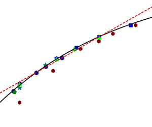
Figure 1 shows comparisons of wall dissipation rates, with the top panels showing the streamwise component and the bottom panels the spanwise component; also shown are the logarithmic growth rates discussed by different authors in the literature. Figure 2 shows similar comparisons for the peak pressure fluctuation (top panels) and the wall pressure fluctuation (bottom panels). Figure 3 shows comparisons of  $u'_p$ (top panels) and
  $w'_p$ (bottom panels). In all these plots, the left-hand panels are for channel and pipe, while the right-hand panels are for TBL. For simplicity of notation, the superscript
  $+$ is omitted from here on unless otherwise specified. The agreement between data and (2.2) is excellent. A quantitative observation for the three flows is that the dissipation component in the
  $z$ direction is about half of that in the
  $x$ direction at the same
  $Re_\tau$; and wall pressure is slightly smaller by 0.4 than the peak pressure, with both pressures of the same order as
  $u'^2_p$ and
  $w'^2_p$.

Figure 1.  $Re_\tau$-variations of wall dissipation rates after normalization in viscous units. Streamwise velocity component
  $\varepsilon _{x-w}$ – equivalently, the fluctuation intensities of streamwise wall shear stress
  $\tau '^{2}_{x-w}$ and spanwise wall vorticity
  $\omega '^2_{z-w}$ – in channel and pipe flows (a) and in TBL flows (b). Spanwise velocity component
  $\varepsilon _{z-w}$ – also the intensities of spanwise wall shear stress
  $\tau '^{2}_{z-w}$ and streamwise wall vorticity
  $\omega '^2_{x-w}$ – in channel and pipe flows (c) and in TBL flows (d). Solid lines are predictions for channel (a,c) and TBL (b,d) by using (2.2), with the parameters summarized in table 1. Dashed lines indicate logarithmic growths in the literature, i.e.
  $\varepsilon _{x-w}=0.02\ln (Re_\tau )+0.035$ by Tardu (Reference Tardu2017) in (a),
  $\varepsilon _{x-w}=0.011\ln (Re_\tau )+0.10$ by Yang & Lozano-Durán (Reference Yang and Lozano-Durán2017) in (b), and
  $\varepsilon _{z-w}=[0.018\ln (Re_\tau )+0.164]^2$ by Diaz-Daniel et al. (Reference Diaz-Daniel, Laizet and Vassilicos2017) in (d), whilst no logarithmic growth for
  $\varepsilon _{z-w}$ in channel/pipe is found in public and hence is absent in (c). Solid symbols are DNS data of channels: star, Moser et al. (Reference Moser, Kim and Mansour1999); pentagon, Orlandi & Leonardi (Reference Orlandi and Leonardi2007); circle, Iwamoto et al. (Reference Iwamoto, Suzuki and Kasagi2002); upward triangle, Hoyas & Jimenez (Reference Hoyas and Jimenez2006); square, Lee & Moser (Reference Lee and Moser2015). For pipes: hexagon, Pirozzoli et al. (Reference Pirozzoli, Romero, Fatica, Verzicco and Orlandi2021). For TBLs: pentagon, Spalart (Reference Spalart1988); diamond, Schlatter et al. (Reference Schlatter, Örlü, Li, Brethouwer, Fransson, Johansson, Alfredsson and Henningson2009). Here and elsewhere, for brevity, symbols are explained in figure legends when they appear for the first time.

Figure 2. Plots of intensities of peak pressure (a,b) and wall pressure (c,d), similar to figure 1. Again, solid lines are fits to (2.2); dashed lines indicate logarithmic growths for wall pressure by Panton et al. (Reference Panton, Lee and Moser2017), i.e.  $p'^2_{w}=2.24\ln (Re_\tau )-9.18$ in (c) for channels and pipes, and
  $p'^2_{w}=2.42\ln (Re_\tau )-8.96$ in (d) for TBLs. Newly included solid symbols are DNS data for pipes (leftward triangle, Wu & Moin (Reference Wu and Moin2008)), for channels (rightward triangle, Yamamoto & Tsuji (Reference Yamamoto and Tsuji2018)) and for TBLs (hexagon, Sillero et al. (Reference Sillero, Jimenez and Moser2013); diamond with cross, Skote (Reference Skote2001)). Other symbols are the same as in figure 1.

Figure 3. The  $Re_\tau$-variations of peak turbulence intensities. Streamwise intensity
  $u'^2_p$ in channel and pipe (a), and in TBL (b). Spanwise intensity
  $w'^2_p$ in channel and pipe (c), and in TBL (d). Newly included data are: EXP pipes of Princeton by Hultmark et al. (Reference Hultmark, Vallikivi, Bailey and Smits2012), of CICLoPE by Willert et al. (Reference Willert, Soria, Stanislas, Klinner, Amili, Eisfelder, Cuvier, Bellani, Fiorini and Talamelli2017) based on PIV measurement, and by Fiorini (Reference Fiorini2017) with hot-wire data corrected; DNS data of pipes by Ahn et al. (Reference Ahn, Lee, Lee, Kang and Sung2015) and of channels by Yao, Chen & Hussain (Reference Yao, Chen and Hussain2019); EXP data of TBL by DeGraaff & Eaton (Reference DeGraaff and Eaton2000), Örlü (Reference Örlü2009), Vincenti et al. (Reference Vincenti, Klewicki, Morrill-Winter, White and Wosnik2013), Marusic et al. (Reference Marusic, Chauhan, Kulandaivelu and Hutchins2015), Vallikivi et al. (Reference Vallikivi, Ganapathisubramani and Smits2015) and Samie et al. (Reference Samie, Marusic, Hutchins, Fu, Fan, Hultmark and Smits2018); see figure legends for the corresponding symbols. Solid lines are fit to (2.2), whose parameters are summarized in table 1. Dashed lines indicate
  $u'^2_{p}=0.63\ln (Re_\tau )+3.8$ by Marusic et al. (Reference Marusic, Baars and Hutchins2017), and
  $w'^2_{p}=0.46\ln (Re_\tau )-1.2$ adopted by us for reference, both of which arise from the Gaussian-logarithmic model for high-order moments, as discussed in the text and shown in figures 4 and 5.
The parameters in (2.2) for the six independent quantities, shown in figures 1–3, form the basis of table 1. Data in figures 1–3 are from the original sources of DNS and EXP measurements (see legends); all available data are included as long as meaningful definition of the peak and wall values are possible. Note that  $\mathcal {D}_{x-w}$ and
  $\mathcal {D}_{z-w}$ would provide another two independent checks of (2.2) but they are not explicitly compared here as their published data are sparser than those in figures 1–3. Moreover,
  $\tau '_{x-w}$,
  $\tau '_{z-w}$,
  $\omega '_{z-w}$ and
  $\omega '_{x-w}$ can be obtained through definitions from mean quantities in table 1, so there is no need to show them separately.
The noteworthy points that emerge from these extensive comparisons are as follows.
(1) The proportionality coefficient
$C_\varPhi$ varies only modestly when the flow direction changes from $x$ to $z$ or from channel and pipe to TBL, implying that essentially the same mechanism applies for all flows.(2) DNS data of pipe follow, overall, the channel data, except for
$\varepsilon _{x-w}$, for which $C_\varPhi$ differs slightly.(3) The fitted
$\varPhi _\infty$ for each mean quantity seems to be universal among channel, pipe and TBL flows, except for differences of the order of 8 % for $\varepsilon _{x-w}$, 2 % for $p'_{p}$ and $p'_{w}$, and 5 % for ${w}'_{p}$, which may be attributed to the uncertainty in transition histories – although we concede the possibility that pipes and channels and TBLs may need to be considered separately if the accuracy of the data improves over time.(4) The fitted
$\varPhi _{\infty }=0.23$ for $\varepsilon _{x-w}$ in TBLs is very close to our theoretical value $1/4$ (validated for $\varepsilon _{x-w}$ in channels and pipes), which bounds the maximum turbulent production.(5) The atmospheric boundary layer measurement over the Salt Lake data of
$p'$ at the wall is reported to be approximately 4.98 at $Re_\tau =10^6$ by Klewicki et al. (Reference Klewicki, Priyadarshana and Metzger2008), 10 % higher than our predicted asymptotic wall pressure $p'_w=4.5$ but agreeing closely with the peak pressure $p'_p=4.95$ (located at $y^+=30$ in viscous units, very close to the wall).(6) The Salt Lake data of
$u'^2_p$ are reported to give around 13.4 with 20 % uncertainty at $Re_\tau =10^6$ (Metzger & Klewicki Reference Metzger and Klewicki2001), overlapping with our estimate of $u'^2_p=11.5$ for asymptotically high $Re_{\tau}$. Thus, from these items (1)–(6), one may regard (2.2) as validated by a large volume of data.


Special attention is drawn to  $u'^2_p$ shown in the top panels of figure 3. In contrast to other quantities, there are notable departures between data and (2.2) for
  $Re_\tau$ less than 500; however, the agreement improves towards higher
  $Re_\tau$. By adjusting
  $\varPhi _\infty =10.5$ and
  $C_\varPhi =12.7$, better agreement can be achieved for smaller
  $Re_\tau$, but these new constants are not as good as the current ones for high
  $Re_\tau$ data. A similar situation is also present in the competing log variation. For example, the log law slope is reported as 0.63 by Marusic et al. (Reference Marusic, Baars and Hutchins2017) for the
  $Re_\tau$ fitting range between 500 and 20 000 (shown in the top panels of figure 3); however, considering
  $Re_\tau$ between 1000 and 5000 only, Lee & Moser (Reference Lee and Moser2015) found the slope as 0.642 for channel and, very recently, Pirozzoli et al. (Reference Pirozzoli, Romero, Fatica, Verzicco and Orlandi2021) found the slope to be 0.612 by choosing a
  $Re_\tau$ range between 180 and 6000 for pipes. Therefore, taking a conservative stance, one cannot yet draw a solid conclusion on the log law slope, nor on the superiority of the competitive log law and (2.2) regarding the ‘correct’
  $u'^2_p$ scaling. Currently, it is unknown whether the departure between the data and different scaling proposals at small Reynolds number is due to transition history, or a physical transition in scaling at a critical
  $Re_\tau \approx 500$. To track this subtle issue, quality data for a one high-quality flow covering both small and large Reynolds number with fine resolution is needed. Another issue is whether channel, pipe and TBL have the same
  $Re_\tau$ scaling for
  $u'^2_p$; this remains unclear, recalling that Samie et al. (Reference Samie, Marusic, Hutchins, Fu, Fan, Hultmark and Smits2018) found the log law slope for TBL as 0.646, larger than all the values obtained for channel and pipe flows.
3. Scaling of velocity fluctuation moments near the wall
It is interesting to examine the scaling of high-order (even) moments of fluctuations, e.g.  $\langle u^{2q} \rangle ^{1/q}$ and
  $\langle w^{2q} \rangle ^{1/q}$ for
  $q=1$ to
  $q=5$. Figure 4(a) shows the wall-normal profiles of fluctuation moments for
  $u$ at
  $Re_\tau =5200$; similarly, figure 5(a) plots moments of
  $w$ for the same
  $Re_\tau$. Near-wall peaks are observed for all these moments, which are obtained from the Johns Hopkins Turbulence Database and contain more than
  $5\times 10^6$ velocity samples. On the basis of scaling considerations similar to those used before, we argue that the maximum values of moments would also be bounded as
  $Re_\tau \rightarrow \infty$, and that the finite-
 $Re_\tau$ dependence is the same
  $1/4$ power. Accordingly, we write
 \begin{equation} \langle \varphi ^{2q} \rangle^{1/q}_{max}=\alpha_q-\beta_q\,Re^{{-}1/4}_\tau, \end{equation}
where  $\varphi$ represents either
  $u$ or
  $w$ fluctuations, and
  $\alpha _q$ represents different asymptotes for different
  $q$ when
  $Re_\tau \rightarrow \infty$;
  $\beta _q$ is independent of
  $Re_\tau$. Note that for
  $q=1$,
  $\alpha _1=\varPhi _\infty$ and
  $\beta _1=C_\varPhi$ in (2.2).

Figure 4. (a) Wall-normal dependence of  $u$-moments at
  $Re_\tau =5200$ in the DNS data of Lee & Moser (Reference Lee and Moser2015). (b)
  $Re_\tau$ variations of the maximum
  $u$ moments near the wall. In (b): solid symbols represent the DNS channel data of Lee & Moser (Reference Lee and Moser2015); open symbols are EXP TBL data by Hutchins et al. (Reference Hutchins, Nickels, Marusic and Chong2009), extracted from Meneveau & Marusic (Reference Meneveau and Marusic2013); and solid lines come from (3.1) in CS, compared with dashed lines from (3.2) and (3.3) by Meneveau & Marusic (Reference Meneveau and Marusic2013).

Figure 5. (a) Wall-normal dependence of  $w$-moments at
  $Re_\tau =5200$. (b)
  $Re_\tau$ variations of the maximum
  $w$ moments near the wall. Data are DNS channel by Lee & Moser (Reference Lee and Moser2015). In (b), solid lines come from (3.1) in CS, compared with dashed lines from (3.2) and (3.3) by Meneveau & Marusic (Reference Meneveau and Marusic2013).
We now consider peaks in various moments of the velocity fluctuations in streamwise directions. Figure 4(b) shows  $Re_\tau$-variations for the near-wall peaks of
  $\langle u^{2q} \rangle ^{1/q}$ for
  $q=1$ to
  $q=5$. Solid lines denote the defect power law fitting by (3.1), where values of
  $\alpha _q$, shown in figure 6(a), are of particular interest because they represent the asymptotic values of
  $\langle u^{2q} \rangle ^{1/q}$. Similarly, figure 5(b) shows the
  $Re_\tau$-variations of the maximum
  $\langle w^{2q} \rangle ^{1/q}$, and the fit to the corresponding
  $\alpha _q$ is shown in figure 6(b). It is clear that (3.1) characterizes the data well, and
  $\alpha _q$ in both cases follows closely a linear relationship with
  $q$. Its underlying explanation will be presented in the next section.


Note for comparison that we include a Gaussian-logarithmic model by Meneveau & Marusic (Reference Meneveau and Marusic2013) (hereafter referred to as MM) in figures 4(b) and 5(b), represented by the dashed lines. The MM model has the dependence
 \begin{equation} \langle \varphi^{2q} \rangle^{1/q}_{max}=A_q\ln (Re_\tau)+K_q, \end{equation}
together with the Gaussian random variable hypothesis for  $\varphi$, yielding
 \begin{equation} A_q=A_1[(q-1)!!]^{1/q} \end{equation}
for the slopes, leaving the intercepts  $K_q$ arbitrary. Figure 4(b) shows that for
  $u$, (3.1) is comparable to the MM model; however, the difference becomes significant for
  $w$ shown in figure 5(b). Overall, the MM model under-predicts the peaks of
  $w$ moments. As noted by Meneveau & Marusic (Reference Meneveau and Marusic2013), sub-Gaussian corrections may be needed to rectify this problem. However, this produces no improvement for
  $q=1$ and does not change the inadequate agreement between data and the log proposal for
  $w'^2_p$; see figure 3(c) for the zoomed-in view. Taken together with plots of the preceding sections, the defect power law (3.1) can be regarded as showing better agreement with data than the Gaussian-logarithmic growth (3.2).
4. Linear $q$-norm Gaussian process

In this section, we show that the linear  $q$-dependence in figure 6 can result from a Gaussian random variable via an exponential transformation.
Let us first define the  $q$-norm for a (random) variable
  $\phi$ as
 \begin{equation} \phi_q=\langle\phi^{q} \rangle^{1/q}, \end{equation}
where  $\langle \cdot \rangle$ here represents the expectation value. If
  $\phi _q$ depends linearly on
  $q$, then it satisfies
 \begin{equation} \phi_q=\ln (\chi_q), \end{equation}
where  $\chi _q$ is the
  $q$-norm of a log-normal variable
  $\chi$, i.e.
  $\chi =e^{\kappa }$ with
  $\kappa$ Gaussian distributed. This is demonstrated as follows.
Given  $\kappa$, one readily obtains
  $\chi _q$ and hence
  $\phi _q$. That is,
 \begin{gather} \chi_q=\langle \chi^{q} \rangle^{1/q}=\langle (e^{\kappa})^{q} \rangle^{1/q}=\langle e^{q\kappa} \rangle^{1/q}, \end{gather}
 \begin{gather} \phi_q=\ln (\chi_q) =\ln (\langle e^{q\kappa} \rangle^{1/q})=(1/q)\ln (\langle e^{q\kappa} \rangle). \end{gather}
Specifically, for a Gaussian variable  $\kappa$ with its mean
  $\mu$ and variance
  $2\sigma$, one has
 \begin{equation} \ln (\langle e^{q\kappa} \rangle)=\mu q +\sigma q^2. \end{equation}
Substitution of (4.5) into (4.3) and (4.4) yields
 \begin{gather} \chi_q=[e^{\mu q +\sigma q^2}]^{1/q}=e^{\mu +\sigma q}, \end{gather}
 \begin{gather} \phi_q=\ln (\chi_q)= \mu +\sigma q. \end{gather}
 We may refer to the random variable  $\phi$ that has a linear
  $q$-norm (4.7) as the ‘linear
  $q$-norm Gaussian’ (LQNG) process generated by the Gaussian seed
  $\kappa$. The above procedure is summarized as follows:
 \begin{equation} \kappa\mathop{\longrightarrow}^{\boldsymbol{E}}\chi\mathop{\longrightarrow}^{\boldsymbol{Q}}\chi_q\mathop{\longrightarrow}^{\boldsymbol{E}^{{-}1}}\phi_q\mathop{\longrightarrow}^{\boldsymbol{Q}^{{-}1}}\phi;\quad \phi=\boldsymbol{Q}^{{-}1}\boldsymbol{E}^{{-}1}\boldsymbol{Q}\boldsymbol{E}(\kappa). \end{equation}
Here,  $\boldsymbol {E}$ and
  $\boldsymbol {Q}$ indicate operations of exponential transform and
  $q$-norm, respectively, which are non-commutable for random variables; and the superscript
  $-1$ indicates the inverse operation (supposing that
  $\phi$ is determined by its moments). In other words, the LQNG process satisfies the operator-reflection symmetry
 \begin{equation} \boldsymbol{E}\circ\boldsymbol{Q}(\phi)=\boldsymbol{Q}\circ\boldsymbol{E}(\kappa). \end{equation}
If  $\phi$ and
  $\kappa$ are non-random, then it is trivial that
  $\phi =\kappa$; instead,
  $\phi$ and
  $\kappa$ here are random variables, and by assigning
  $\kappa$ as a Gaussian variable, we obtain a linear dependence of
  $\phi _q$ on
  $q$.
$q$.
For wall turbulence, the asymptotes for the near-wall peaks of  $\langle u^{2q} \rangle ^{1/q}$ and
  $\langle w^{2q} \rangle ^{1/q}$ when
  $Re_\tau \rightarrow \infty$ are LQNG processes. That is, substituting
  $\phi =u^{2}$ in (4.7) gives
 \begin{equation} \alpha_{u,q}=\mu_u +\sigma_u q, \end{equation}
where  $\mu _u\approx 5.5$ and
  $\sigma _u\approx 5.9$ according to figure 6(a). Similarly, substituting
  $\phi =w^{2}$ in (4.7) gives
 \begin{equation} \alpha_{w,q}=\mu_w +\sigma_w q, \end{equation}
where  $\mu _w\approx 0$ and
  $\sigma _w\approx 3.9$ according to figure 6(b). The fact that
  $\mu _w \approx 0$ may reflect the absence of inactive motion in the
  $w$-component of the velocity.
5. Discussion on data quality
Presently, the range of high-quality and accurate experimental data remains limited, particularly with respect to the verification of the scaling of  $u'_p$ and
  $p'_p$, and greater certainty will be possible only as better data become available. However, for
  $w'_p$ and the wall dissipation, the two competing scaling proposals (i.e.
  $1/4$ defect power law and the log law) already show notable differences in the
  $Re_\tau$ domain up to
  $10^4$. Hence a cogent scaling verification for
  $w'_p$,
  $\varepsilon _{x-w}$ and
  $\varepsilon _{z-w}$ may already be on hand. In saying this, we assume that the present data on
  $w'_p$,
  $\varepsilon _{x-w}$ and
  $\varepsilon _{z-w}$ are of adequate accuracy, but the veracity of data is clearly the ultimate arbiter.
For the DNS data, a particular point is that different grid resolutions may influence statistics. As shown by Yang et al. (Reference Yang, Hong, Lee and Huang2021), to capture the extreme events of wall dissipation, very fine resolution is needed even at a moderate  $Re_\tau$, similar to the effect known for homogeneous and isotropic turbulence; see, for example, Yeung, Sreenivasan & Pope (Reference Yeung, Sreenivasan and Pope2018). This brings up the question of data uncertainty, which, of course, is always deserving of attention; see Monkewitz (Reference Monkewitz2021) for more discussions.
One may alternatively use indirect methods to estimate wall dissipation, e.g.  $\varepsilon _{x-w}\approx (u'/U)^2$ (or
  $(u'/y)^2$) and
  $\varepsilon _{z-w}\approx (w'/U)^2$ (or
  $(w'/y)^2$) towards the wall. These near-wall Taylor expansions are technically correct for
  $y^+\rightarrow 0$, but may introduce uncertainty in practice because of the finite grid. For example, figure 7(a) shows that the
  $(u'/U)^2$ values (half-open hexagons) at
  $y^+$ locations closest to the wall for the DNS data of Pirozzoli et al. (Reference Pirozzoli, Romero, Fatica, Verzicco and Orlandi2021) are noticeably higher than the wall values of
  $\varepsilon _{x-w}$ (solid hexagons). Such a difference could also be related to specific numerical schemes used in DNS. The difference is smaller and negligible for the data of Lee & Moser (Reference Lee and Moser2015) and of Hoyas & Jimenez (Reference Hoyas and Jimenez2006), both sources having used the spectral method; see half-open symbols in figure 7. Therefore the linear approximation by Taylor expansion agrees well in some simulations, but not in others. In any case, if one utilizes this extrapolation method to estimate
  $\varepsilon _{x-w}$ in the absence of direct measurements of the wall dissipation, the open symbols in figure 7(a) result. One may even infer a log variation from these open symbols when the significant data scatter is ignored. However, for these same DNS data sets without direct measurements of
  $\varepsilon _{z-w}$, figure 7(b) shows
  $(w'/U)^2$ towards the wall following the
  $1/4$ defect power law closely. Despite this agreement, all the issues on data uncertainty (including numerical schemes in DNS, hot-wire resolution in EXP, indirect estimation, etc.) need careful examination and are left for future examination.

Figure 7. Same plots as figure 1(a,c), with newly added symbols (see legends) for wall values of  $(u'/U)^2$ and
  $(w'/U)^2$ as approximations for
  $\varepsilon _{x-w}$ (a) and
  $\varepsilon _{z-w}$ (b), respectively. Solid lines are channel flow predictions according to (2.2), with the parameters summarized in table 1. Dashed lines indicate, for reference, the logarithmic growths, i.e.
  $0.0202\ln (Re_\tau )+0.045$ in (a) and
  $0.008\ln (Re_\tau )+0.0216$ in (b). Solid symbols represent wall dissipation, and are the same DNS data as in figure 1. Newly included half-open symbols are the DNS data. For channels: triangle, Hoyas & Jimenez (Reference Hoyas and Jimenez2006); square, Lee & Moser (Reference Lee and Moser2015). For pipes: hexagon, Pirozzoli et al. (Reference Pirozzoli, Romero, Fatica, Verzicco and Orlandi2021). Newly included open symbols are from the DNS data (the wall dissipation rates being absent). For channels: circle, Bernardini, Pirozzoli & Orlandi (Reference Bernardini, Pirozzoli and Orlandi2014); diamond, Lozano-Durán & Jimenez (Reference Lozano-Durán and Jimenez2014); rightward triangle, Yamamoto & Tsuji (Reference Yamamoto and Tsuji2018). For pipes: leftward triangle, Wu & Moin (Reference Wu and Moin2008).
Since the available  $Re_\tau$ domain is not large, it is not surprising that other formula may fit data similarly well. For example, recalling the comparison for
  $p'_w$ in figure 2, where the defect power law is indistinguishable from the square root of logarithmic growth, one may use
  $\varPhi =\sqrt {A\ln Re_\tau +B}$ (where
  $A$ and
  $B$ are coefficients) to represent the wall dissipation rate. Similarly, if we change the scaling exponent of
  $-1/4$ and the proportional coefficient in (2.2) by
  $1/4-\varepsilon _{x-w}\approx 0.38Re_\tau ^{-1/4.3}$ or
  $0.48 Re_\tau ^{-1/3.7}$, both of them fit the data well. We should point out, however, that the rationale for these alternative proposals is absent.
So far, the above scaling relations are derived from consideration of how the wall dissipation departs from its presumed limit. It would be interesting to examine the relation between the wall dissipation defect and modulations imposed by the large-scale motions further away from the wall (Metzger & Klewicki Reference Metzger and Klewicki2001; Mathis, Hutchins & Marusic Reference Mathis, Hutchins and Marusic2009). A phenomenological model such as the hierarchical random additive process (Yang & Lozano-Durán Reference Yang and Lozano-Durán2017) might be insightful in explaining how the wall-attached eddies are related to the various bounds proposed here. In this context, one may wonder why growing eddies lead to saturated wall fluctuations. A plausible answer is that the increasing contributions by these eddies are exactly accounted for by the normalization in  $u_\tau$, with the inactive motions becoming decreasingly influential. This is simply reminiscent of the Reynolds shear stress
  $\langle -uv \rangle$ and Reynolds normal stress
  $\langle vv \rangle$, referred to as the active motions by Townsend (Reference Townsend1956), whose magnitudes are also thought to be bounded after scaling in wall units.
Additional comments may now be made regarding the scaling of active motions. In particular, the magnitudes of peak  $\langle -uv \rangle$ and peak
  $\langle vv\rangle$ have been thought to obey – with theoretical support from the log law mean velocity (see Sreenivasan Reference Sreenivasan1989; Pirozzoli et al. Reference Pirozzoli, Romero, Fatica, Verzicco and Orlandi2021; Smits et al. Reference Smits, Hultmark, Lee, Pirozzoli and Wu2021) – the defect power law
  $1- \langle -uv \rangle ^+_p \propto Re_\tau ^{-1/2}$. However, a recent study by Chen, Hussain & She (Reference Chen, Hussain and She2019) shows that
  $1- \langle -uv \rangle ^+_p$ exhibits different scaling transitions for channel/pipe on the one hand, and TBL flows on the other. Specifically,
  $1- \langle -uv \rangle ^+_p \propto Re_\tau ^{-2/3}$ for
  $Re_\tau < 1000$, and
  $1- \langle -uv \rangle ^+_p \propto Re_\tau ^{-1/2}$ for higher-
 $Re_\tau$ channel/pipe flows. The present paper focuses on wall values or near-wall fluctuations with invariant peak locations (e.g. for
  $u'$,
$u'$,  $w'$ and
  $p'$), hence differing from the active motions (e.g.
  $\langle -uv \rangle$) extending infinitely far away from the wall (in
  $y^+$ units) as
  $Re_\tau$ increases. This is perhaps why they exhibit different defect power law exponents.
6. Conclusion
For the last three decades, considerable effort has been devoted to understanding the  $Re_\tau$ growth of peak values of turbulent fluctuations, mostly based on the logarithmic form that shows an unbounded growth, thus indicating the breakdown of the wall scaling for turbulence fluctuations. While different arguments can, in fact, be invoked in those logarithmic descriptions, deviations from the log fits can be observed for
  $\varepsilon _{x-w}$,
  $\varepsilon _{z-w}$ and
  ${w'}_p$ in figures 1 and 3. The alternative (2.2) presented in this paper has shown that the averages of turbulent fluctuations – such as the intensities of wall shear stress, wall vorticity components, wall pressure, and intensity peaks of streamwise velocity, spanwise velocity and pressure, all of which possess non-zero wall values or near-wall peaks – follow a universal
  $Re_\tau ^{-1/4}$ defect law. The underlying physics is that the maximum turbulent production provides a bounding constraint on the dissipation rate, and in turn on all near-wall quantities in the limit of infinite Reynolds number. What matters at any finite Reynolds number is the departure of the dissipation rate from its limiting value, as explained in CS. We have simply devised a way to describe the finite
  $Re_\tau$ correction as this asymptote is reached. The present proposal is validated against a large set of flow data.
The paper also extends the same argument to wall-normal peaks in high-order (even) moments of fluctuations. We have also produced a model that describes the variation of these higher moments of fluctuations. Together, the results support the classical wall scaling and indicate a bounded ultimate near-wall turbulence state. That is, moments of near-wall turbulence fluctuations, when suitably normalized by wall variables, attain constant values asymptotically at infinitely large Reynolds numbers. We believe that this is a significant conclusion.
Acknowledgements
We thank all the authors cited in figures 1–7 for making their data available, and particularly thank one of the referees on discussions about the linear approximation method in figure 7 for estimating the wall dissipation rate. For figures 4 and 5, we appreciate the help of T. Zaki and Y. Ji for accessing the Johns Hopkins Turbulence Database (http://turbulence.pha.jhu.edu) for large  $Re_\tau$ data, and the help of J. Yao for small
  $Re_\tau$ data – all are obtained from the DNS code by M. Lee and R.D. Moser. Correspondence with P.A. Monkewitz, H.M. Nagib and A.J. Smits is gratefully acknowledged.
Funding
X.C. acknowledges support from the National Natural Science Foundation of China, grant nos. 12072012, 11721202 and 91952302.
Declaration of interests
The authors report no conflict of interest.


