


1. Introduction
The characterization and modelling of wall-bounded turbulent flows is of paramount importance in physics and engineering (Marusic, Mathis & Hutchins Reference Marusic, Mathis and Hutchins2010). Organized motions, in particular, play a crucial role in wall-bounded turbulence analysis, because they are associated with high-energy levels and are directly involved in transport processes, which make them preferential targets for flow control strategies (Jiménez Reference Jiménez2018). Coherent streaks are recognized as the dominant flow structures very close to the wall, and are characterized by a distinctive (inner) peak in the spectrogram of the streamwise velocity fluctuations,  $u$, within the buffer layer (Jiménez Reference Jiménez2018). The investigation of high-Reynolds-number experiments and simulations also reveal the formation of large-scale motions (LSMs) and very-large-scale motions (VLSMs) that reside in the log region (Smits, McKeon & Marusic Reference Smits, McKeon and Marusic2011), whose presence is detected by the appearance of another (outer) peak in the (pre-multiplied) energy spectrogram of the streamwise velocity fluctuations (Hutchins & Marusic Reference Hutchins and Marusic2007b; Monty et al. Reference Monty, Hutchins, Ng, Marusic and Chong2009; Peruzzi et al. Reference Peruzzi, Poggi, Ridolfi and Manes2020). The wall-normal location in wall units (i.e. made dimensionless by the mean friction velocity,
  $U_\tau$, and the fluid kinematic viscosity,
  $\nu$),
  $y^+=yU_\tau /\nu$, of the inner peak is conventionally assumed to be fixed at
  $y^+=15$, while the position of the outer peak increases with the frictional Reynolds number,
  ${\textit {Re}}_\tau$, as
  $y^+\approx 3.9{\textit {Re}}_\tau ^{1/2}$ (Mathis, Hutchins & Marusic Reference Mathis, Hutchins and Marusic2009a).
In addition to the effect of the Reynolds number, some differences emerge from the comparison of different canonical wall-bounded turbulent flows. While near-wall statistics (such as the mean velocity profile) agree well in channel, pipe and boundary layer flows, the features of the large scales depend on the flow configuration (Balakumar & Adrian Reference Balakumar and Adrian2007; Monty et al. Reference Monty, Stewart, Williams and Chong2007; Mathis et al. Reference Mathis, Monty, Hutchins and Marusic2009b; Monty et al. Reference Monty, Hutchins, Ng, Marusic and Chong2009; Chernyshenko Reference Chernyshenko2020). In particular, spectral analyses of internal and external flows have revealed that the very-large scales tend to be longer for channel and pipe flows than boundary layer flows, although they appear to be qualitatively similar (Balakumar & Adrian Reference Balakumar and Adrian2007; Monty et al. Reference Monty, Hutchins, Ng, Marusic and Chong2009). Such large-scale differences are expected to increase for larger Reynolds numbers as energetic contributions resulting from VLSM increases with the Reynolds number.
The investigation of higher Reynolds number data has progressively revealed novel developments and questions concerning the interaction between the small-scale turbulence (whose spectral peak occurs in the proximity of the wall) and LSMs (whose spectral peak resides far from the wall). Insights on scale interaction were initially reported by Brown & Thomas (Reference Brown and Thomas1977) and Bandyopadhyay & Hussain (Reference Bandyopadhyay and Hussain1984), who observed a modulation mechanism on the (near-wall) small scales by the large turbulent scales. Later, Hutchins & Marusic (Reference Hutchins and Marusic2007b) provided further evidence of a top-down footprint and an AM phenomenon by the large scales residing in the log region on the near-wall (small-scale) dynamics. With the aim to illustrate such an inter-scale mechanism, figure 1(a) shows a schematic of a wall-bounded turbulent flow in a streamwise-vertical plane, where uniform momentum regions arising from LSM and VLSM (highlighted as dark- and light-blue structures) entail large-scale fluctuations,  $u_{LS}$ (see red lines). Figure 1(a) is drawn following the current picture of the kinematics of turbulent scales and their interaction in wall-bounded turbulence (e.g. see Ganapathisubramani et al. Reference Ganapathisubramani, Hutchins, Monty, Chung and Marusic2012; Baars, Hutchins & Marusic Reference Baars, Hutchins and Marusic2017). The turbulent flow field can be decomposed as
  $u(x,y,z,t)=u_{LS}(x,y,z,t)+u_{SS}(x,y,z,t)$, where
  $u_{SS}$ are small-scale fluctuations (see black signals), while
  $x,y,z$ are the streamwise, vertical and spanwise directions, respectively, and
  $t$ is the time. Figure 1(a) also highlights the top-down footprint of the large scales, being the two
  $u_{LS}$ signals (red lines) positively correlated with each other (eventually accounting for the inclination of the large scales Marusic & Heuer Reference Marusic and Heuer2007).
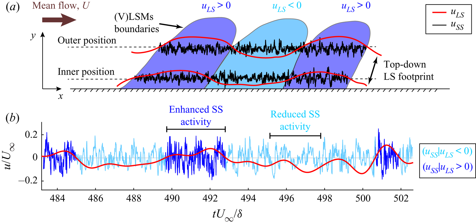
Figure 1. (a) Schematic of a wall-bounded turbulent flow in the  $(x$–
$(x$– $y)$ plane, showing three alternating LSM and VLSM structures of uniform large-scale momentum,
  $u_{LS}\lessgtr 0$. Two pairs of time series of
  $u_{LS}$ and
  $u_{SS}$ are also depicted as red and black lines, respectively, at two wall-normal locations (referred to as the inner and outer positions). (b) Small-scale,
  $u_{SS}$, and large-scale,
  $u_{LS}$, streamwise velocity fluctuations at
  $y^+\approx 10$, shown as blue and red lines, respectively, where the light- and dark-blue portions of
  $u_{SS}$ correspond to intervals of
  $u_{LS}<0$ and
  $u_{LS}>0$, respectively. The velocity series is extracted from an experimental turbulent boundary layer at
  ${\textit {Re}}_\tau =14\,750$ (Marusic Reference Marusic2020) in the range
  $tU_\infty /\delta =483\text {--}503$, where
  $U_\infty$ and
  $\delta$ are the free stream velocity and boundary layer thickness, respectively. Two intervals of the signal (i.e.
  $490<t U_\infty /\delta <493$ and
  $495<t U_\infty /\delta <498$), in which the small scales display enhanced or reduced activity, are also indicated.
A modulation of the amplitude of the small scales caused by the large scales implies that high or low values of  $u_{LS}$ correspond to (on average) high or low values of
  $u_{SS}$. This mechanism can be observed in figure 1(b), which shows time intervals of
  $u_{LS}$ and
  $u_{SS}$ at
  $y^+\approx 10$ in an experimental turbulent boundary layer. An increase of the local amplitude of the small-scale signal (see dark-blue intervals) is discernible during positive large-scale velocity fluctuations,
  $u_{LS}>0$, and, vice versa, a damping of the small-scale amplitudes (light-blue intervals) is evident during negative large-scale velocity fluctuations,
  $u_{LS}<0$.
Mathis et al. (Reference Mathis, Hutchins and Marusic2009a) quantified this AM by correlating  $u_{LS}$ with the large-scale-filtered envelope of
  $u_{SS}$ at different wall-normal coordinates. The authors observed an AM (as shown in figure 1b) only close to the wall (approximatively below the centre of the log region), while a reversed AM mechanism – i.e. an
  $u_{SS}$ amplitude increase under
  $u_{LS}<0$ and an
  $u_{SS}$ amplitude decrease under
  $u_{LS}>0$ – occurred far from the wall. Further studies on turbulent boundary layers have suggested that a modulation mechanism does actually take place only in the near-wall region, while different mechanisms occur in the log and wake regions. In particular, the behaviour of the scale interaction away from the wall has been explained either through a preferential arrangement of the small scales – i.e. an alignment of the small-scale turbulence with internal shear layers that separate zones of large-scale uniform momentum (Hutchins Reference Hutchins2014; Baars et al. Reference Baars, Hutchins and Marusic2017) – or as an effect of variations in the mean strain and in the shear-driven production (Agostini & Leschziner Reference Agostini and Leschziner2019).
Based on the insights from Hutchins & Marusic (Reference Hutchins and Marusic2007b) and Mathis et al. (Reference Mathis, Hutchins and Marusic2009a), AM has been widely investigated for several flow configurations and Reynolds numbers, both experimentally (e.g. see Mathis et al. Reference Mathis, Monty, Hutchins and Marusic2009b; Schlatter & Örlü Reference Schlatter and Örlü2010; Guala, Metzger & McKeon Reference Guala, Metzger and McKeon2011; Ganapathisubramani et al. Reference Ganapathisubramani, Hutchins, Monty, Chung and Marusic2012; Talluru et al. Reference Talluru, Baidya, Hutchins and Marusic2014; Baars et al. Reference Baars, Talluru, Hutchins and Marusic2015; Duvvuri & McKeon Reference Duvvuri and McKeon2015; Squire et al. Reference Squire, Baars, Hutchins and Marusic2016; Baars et al. Reference Baars, Hutchins and Marusic2017; Pathikonda & Christensen Reference Pathikonda and Christensen2017; Basley, Perret & Mathis Reference Basley, Perret and Mathis2018; Pathikonda & Christensen Reference Pathikonda and Christensen2019) and via numerical simulations (e.g. see Chung & McKeon Reference Chung and McKeon2010; Bernardini & Pirozzoli Reference Bernardini and Pirozzoli2011; Agostini & Leschziner Reference Agostini and Leschziner2014; Agostini, Leschziner & Gaitonde Reference Agostini, Leschziner and Gaitonde2016; Anderson Reference Anderson2016; Hwang et al. Reference Hwang, Lee, Sung and Zaki2016; Yao, Huang & Xu Reference Yao, Huang and Xu2018; Agostini & Leschziner Reference Agostini and Leschziner2019; Dogan et al. Reference Dogan, Örlü, Gatti, Vinuesa and Schlatter2019). Furthermore, findings on scale interactions have fostered the development of predictive models for near-wall turbulence that explicitly account for the footprint and AM by the large scales on the small scales (Marusic et al. Reference Marusic, Mathis and Hutchins2010; Mathis, Hutchins & Marusic Reference Mathis, Hutchins and Marusic2011; Mathis et al. Reference Mathis, Marusic, Chernyshenko and Hutchins2013; Baars, Hutchins & Marusic Reference Baars, Hutchins and Marusic2016; Wu, Christensen & Pantano Reference Wu, Christensen and Pantano2019). It should be noted that, although large-scale spectral features do not match between internal and external flows, similar AM results have been found for channel, pipe and boundary layer flows at similar  ${\textit {Re}}_\tau$ values (Mathis et al. Reference Mathis, Monty, Hutchins and Marusic2009b), which suggest a similar scale-interaction mechanism is at play in all configurations.
In addition to AM, small-scale turbulence has also been found to change its instantaneous (i.e. local) frequency during intervals of positive or negative  $u_{LS}$, namely the large scales affect the small scales through a frequency modulation (FM) mechanism (Ganapathisubramani et al. Reference Ganapathisubramani, Hutchins, Monty, Chung and Marusic2012; Baars et al. Reference Baars, Talluru, Hutchins and Marusic2015; Fiscaletti, Ganapathisubramani & Elsinga Reference Fiscaletti, Ganapathisubramani and Elsinga2015). However, only a few investigations to quantify FM in wall-bounded turbulence have been carried out so far (Ganapathisubramani et al. Reference Ganapathisubramani, Hutchins, Monty, Chung and Marusic2012; Baars et al. Reference Baars, Talluru, Hutchins and Marusic2015, Reference Baars, Hutchins and Marusic2017; Pathikonda & Christensen Reference Pathikonda and Christensen2017; Awasthi & Anderson Reference Awasthi and Anderson2018; Tang & Jiang Reference Tang and Jiang2018; Pathikonda & Christensen Reference Pathikonda and Christensen2019) when compared with the vast literature on AM and its application into predictive models. One of the main reasons for this literature imbalance resides on the difficulty to produce robust methodologies to quantify FM in broadband signals, as well as the difficulty to effectively capture instantaneous frequencies in a signal.
With the aim to quantify FM in the context of a wall-bounded turbulence scale interaction, two methodologies have been proposed so far. Ganapathisubramani et al. (Reference Ganapathisubramani, Hutchins, Monty, Chung and Marusic2012) proposed a peak–valley approach, following the idea that the local frequency is proportional to the number of maxima and/or minima per unit length of the series. The peak–valley approach was applied to streamwise  $u_{SS}$ signals from experimental measurements in a turbulent boundary layer at
  ${\textit {Re}}_\tau =\delta U_\tau /\nu =14\,150$ (where
  $\delta$ is the boundary layer thickness). Similar to AM, the authors found a relevant FM of the small scales in the near-wall region in which higher frequencies correspond to large (positive)
  $u_{LS}$ values while lower frequencies correspond to low (negative)
  $u_{LS}$ values. However, different from AM, substantial FM was observed only up to
  $y^+\approx 100$. As an example of this FM mechanism, in figure 1(b), a rapidly fluctuating
  $u_{SS}$ activity can be seen during positive
  $u_{LS}$ (dark-blue intervals) rather than negative
  $u_{LS}$ (light blue intervals). Despite its conceptual simplicity, the main drawback of the peak–valley approach is the need of a signal discretization into sub-intervals of arbitrary spacing to quantify the number of maxima and minima within each sub-interval. The choice of the size of the signal partition into sub-intervals is non-trivial and requires a trade-off between too short or too large intervals that can affect the results. Moreover, as pointed out by Baars et al. (Reference Baars, Talluru, Hutchins and Marusic2015), the short-time partitioning of the peak–valley approach makes it less applicable if a focus on temporal shifts in AM and FM is required.
An alternative approach to quantify FM and effectively account for time shifts was then proposed by Baars et al. (Reference Baars, Talluru, Hutchins and Marusic2015), who exploited wavelet analysis to extract from the velocity time series a new signal that is representative of the local frequency variations at the small scales. The authors performed a time–frequency analysis of the streamwise velocity, in which a time series – representative of the small-scale instantaneous frequency – was obtained by evaluating the first spectral moment of the wavelet power spectrum, namely an average energetic contribution at each time for the range of (high) frequencies pertaining the small scales (Baars et al. Reference Baars, Talluru, Hutchins and Marusic2015). The first spectral moment was eventually long-pass filtered to retain only its large-scale component, and correlated with  $u_{LS}$ to quantify FM (similar to the AM technique proposed by Mathis et al. Reference Mathis, Hutchins and Marusic2009a).
The wavelet-based procedure was applied to experimental streamwise velocity time series measured at different wall-normal locations from a turbulent boundary layer at  ${\textit {Re}}_\tau =14\,750$ (Baars et al. Reference Baars, Talluru, Hutchins and Marusic2015). The authors showed positive correlations up to the centre of the log region, which meant that higher and lower frequencies in
  $u_{SS}$ were detected under
  $u_{LS}>0$ and
  $u_{LS}<0$, respectively. Almost zero correlations were observed, instead, for higher wall-normal locations up to the boundary layer intermittent region, where negative correlation values were detected. The near-wall FM found by Baars et al. (Reference Baars, Talluru, Hutchins and Marusic2015) is in accordance with the outcomes from Ganapathisubramani et al. (Reference Ganapathisubramani, Hutchins, Monty, Chung and Marusic2012), but the
  $y^+$ coordinate above which FM was found to be almost absent is larger by using the wavelet-based approach (
 $y^+\approx 470$) compared with that obtained by the peak–valley approach (
 $y^+\approx 100$), although the
  ${\textit {Re}}_\tau$ values were rather similar. Furthermore, a phase lead of the small-scale amplitude and frequency was found in the near-wall with respect to the large-scale signals, and – in accordance with previous studies (Bandyopadhyay & Hussain Reference Bandyopadhyay and Hussain1984; Guala et al. Reference Guala, Metzger and McKeon2011) – a much larger lead was detected for the small-scale amplitudes than for frequency. Although the FM has been accepted as a near-wall mechanism, the interaction mechanism in terms of FM between the small and large scales in the log and wake regions has not been completely clarified, in particular, the precise wall-normal coordinate at which the small-scale frequency is no longer affected by the large scales needs to be determined.
So far, the wavelet-based technique by Baars et al. (Reference Baars, Talluru, Hutchins and Marusic2015) has been exploited as the main tool to quantify FM in wall-bounded turbulence. Different flow configurations have been explored in terms of FM, such as experimental smooth-wall turbulent boundary layers via hot-wire measurements (Baars et al. Reference Baars, Hutchins and Marusic2017) and particle image velocimetry (Pathikonda & Christensen Reference Pathikonda and Christensen2019), experimental boundary layers in the presence of wall roughness (Pathikonda & Christensen Reference Pathikonda and Christensen2017; Tang & Jiang Reference Tang and Jiang2018), as well as large-eddy simulation of a turbulent channel flow with spanwise heterogeneity (Awasthi & Anderson Reference Awasthi and Anderson2018). These works highlighted that, despite the specific quantitative differences, near-wall FM is present both for smooth and rough walls, as well as for several Reynolds numbers. However, despite its preferred employment for quantifying FM, the wavelet-based approach presents some criticalities. First, as discussed by Baars et al. (Reference Baars, Talluru, Hutchins and Marusic2015), the choice of the mother wavelet can have an impact on the results because different frequency resolutions are gained from different mother wavelets. Moreover, the procedure necessitates multiple filtering operations that demand the choice of an appropriate frequency filter value. In particular, a frequency threshold is required both in the computation of the first spectral moment of the wavelet power spectrum (which involves a numerical integration) and in the long-pass filtering of the first spectral moment. Therefore, different from the peak–valley approach of Ganapathisubramani et al. (Reference Ganapathisubramani, Hutchins, Monty, Chung and Marusic2012), in which maxima and minima are counted, the wavelet-based approach intrinsically requires several procedural steps and assumptions that need to be carefully handled.
In this work, a novel approach to study FM in wall-bounded turbulence is put forward with a twofold aim: (i) to propose a non-parametric and robust methodology to extract local frequency changes in a signal; and (ii) to show its effectiveness for two wall-bounded turbulence configurations, as well as to report novel insights that can help to further shed light on the large–small-scale interaction. Our methodology relies on the natural visibility graph (NVG) approach proposed by Lacasa et al. (Reference Lacasa, Luque, Ballesteros, Luque and Nuno2008), which is used to map a signal into a network by exploiting a geometrical criterion. Thanks to its simplicity of implementation, the NVG has been widely employed in a variety of research areas such as, among many others, economy, biomedicine and geophysics (Zou et al. Reference Zou, Donner, Marwan, Donges and Kurths2018). In particular, visibility-based investigations have been carried out in fluid mechanics to study jets and fires (Charakopoulos et al. Reference Charakopoulos, Karakasidis, Papanicolaou and Liakopoulos2014; Murugesan, Zhu & Li Reference Murugesan, Zhu and Li2019; Tokami et al. Reference Tokami, Hachijo, Miyano and Gotoda2020), wall-bounded turbulent flows (Liu, Zhou & Yuan Reference Liu, Zhou and Yuan2010; Iacobello, Scarsoglio & Ridolfi Reference Iacobello, Scarsoglio and Ridolfi2018b), passive scalar plumes (Iacobello et al. Reference Iacobello, Ridolfi, Marro, Salizzoni and Scarsoglio2018a, Reference Iacobello, Marro, Ridolfi, Salizzoni and Scarsoglio2019a) and turbulent combustors (Murugesan & Sujith Reference Murugesan and Sujith2015, Reference Murugesan and Sujith2016; Singh et al. Reference Singh, Belur Vishwanath, Chaudhuri and Sujith2017).
In spite of its simplicity, the NVG approach (defined in § 2.1) has been shown to be a powerful tool in capturing important features of the mapped signal (such as the occurrence of extreme events) and as a reliable indicator of the transition between different flow dynamics (Iacobello, Ridolfi & Scarsoglio Reference Iacobello, Ridolfi and Scarsoglio2021). Here we show that the degree centrality, which is one of the simplest network metrics, is much more sensitive to the small-scale spectral energy variations than their large-scale counterpart (2.2). Accordingly, the network degree is viewed as a metric that is able to inherit the local frequency variations in a signal (2.3), without any a priori assumption (e.g. signal filtering). Therefore, the NVG approach can be directly used to study the full velocity signals rather than the small-scale component.
The proposed NVG approach is used to analyse the time series (§ 3.2) from an experimental smooth-wall zero-pressure-gradient turbulent boundary layer ( ${\textit {Re}}_\tau =14\,750$, Marusic Reference Marusic2020), and the spatial series – namely one-dimensional (1-D) signals along spatial transects at a fixed time (§ 3.1) – from two direct numerical simulations (DNSs) of smooth-wall incompressible turbulent channel flows (
 ${\textit {Re}}_\tau \approx 5200$ and
  ${\textit {Re}}_\tau = 1000$, Lee & Moser Reference Lee and Moser2015; Graham et al. Reference Graham2016). In this regard, for simplicity, we refer FM to indicate both temporal and spatial frequency (i.e. wavenumber) modulation, where the former applies to the time series while the latter to the spatial series. A comparative FM analysis is performed by highlighting the differences and similarities between outcomes from the two wall-bounded turbulence set-ups for the streamwise velocity (§ 4.1). In particular, the effect of different Reynolds numbers is examined, and the application of Taylor's hypothesis to the time series is discussed by proposing a convection velocity that compensates for the overprediction of the modulation in the near-wall region. Moreover, FM results are examined, in view of the quasi-steady quasi-homogeneous theory, in terms of degree centrality scaling with respect to the large-scale velocity values (§ 4.2). The analysis is then extended to the wall-normal and spanwise velocities of the channel flow (§ 4.3), and the time and space shifts are eventually investigated for all the three velocity components (§ 4.4). Finally, we provide a discussion on some general features of the visibility approach (§ 5) as well as concluding remarks (§ 6).
2. Visibility-based analysis of frequency modulation
2.1. Definition of visibility graph
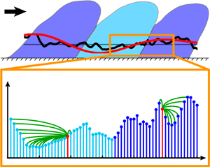
Visibility graphs represent a widely employed technique to map a discrete signal in a network. The idea behind the visibility graph approach is to assign a node of the network to each datum in the signal, and activate a link between two nodes if a geometrical criterion is satisfied. The main variant is the NVG, which is based on a convexity criterion (Lacasa et al. Reference Lacasa, Luque, Ballesteros, Luque and Nuno2008). Geometrically, two nodes in an NVG (corresponding to two points in the signal) are linked if the straight line connecting the two points lies above any other in-between data. Figure 2(a, lower diagram) shows an example of a short series,  $s_i\equiv s(\chi _i)$, for the independent variable
  $\chi _i$ (i.e. a time or space coordinate), comprising
  $N=20$ observations, illustrated as vertical bars. Nodes and links in figure 2(a) are depicted as filled circles at the tip of each bar and green straight lines, respectively. A representative node is highlighted in red and its links are reported in orange.
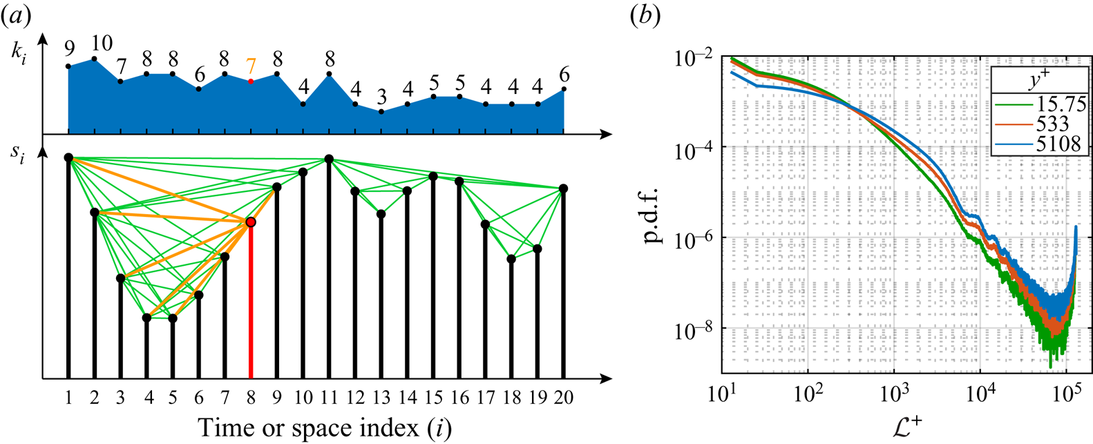
Figure 2. (a) The lower diagram shows an example of a signal,  $s_i\equiv s(\chi _i)$, and the corresponding visibility network, where nodes are depicted as black filled circles and links as green lines. In particular, the node
  $i=8$ and its links are highlighted in orange. The degree values for each node,
  $k_i$, are also shown in the upper diagram. (b) Probability density function (PDF) of the link length evaluated on the network built from the streamwise velocity,
  $u(x)$, in a turbulent channel flow at
  ${\textit {Re}}_\tau \approx 5200$. The link length is expressed in wall units as
  $\mathcal {L}^+=|i-j|{\rm \Delta} x^+$, where
  $i$ and
  $j$ are the indices of two connected nodes and
  ${\rm \Delta} x^+=12.7$ (see § 3.1).
The NVG criterion applied to a generic signal,  $s(\chi )$, can be formally written as
 \begin{equation}
s(\chi_n)<s(\chi_j)+(s(\chi_i)-s(\chi_j))
\frac{\chi_j-\chi_n}{\chi_j-\chi_i},\quad i,j=1,\ldots,N,
\end{equation}
\begin{equation}
s(\chi_n)<s(\chi_j)+(s(\chi_i)-s(\chi_j))
\frac{\chi_j-\chi_n}{\chi_j-\chi_i},\quad i,j=1,\ldots,N,
\end{equation}
for any  $\chi _n$ (i.e. time or space coordinate) such that
  $\chi _i<\chi _n<\chi _j$ (Lacasa et al. Reference Lacasa, Luque, Ballesteros, Luque and Nuno2008). The corresponding visibility network is represented through the adjacency (binary) matrix
  $\boldsymbol {A}$, whose entries are
  $A_{i,j}=1$ if the inequality (2.1) is satisfied for the node pair
  $(i,j)$ with
  $i\neq j$, and
  $A_{i,j}=0$ otherwise. For example, in figure 2(a), the node
  $i=8$ is connected (i.e.
  $A_{8,j}=1$) to nodes
  $j=\lbrace 1, 2, 3, 4, 5, 7, 9\rbrace$, as highlighted by the orange links. By definition, visibility networks are connected (i.e. each node
  $i$ is linked to at least one other node
  $j$, e.g.
  $j=i+1$ or
  $j=i-1$) and undirected (Newman Reference Newman2018), namely the adjacency matrix is symmetric (
 $A_{i,j}=A_{j,i}$).
Different from other techniques developed to transform a signal into a network (Zou et al. Reference Zou, Donner, Marwan, Donges and Kurths2018; Iacobello et al. Reference Iacobello, Ridolfi and Scarsoglio2021), the visibility algorithm does not require any a priori parameters. Given a signal, a unique visibility network is obtained in a straightforward way by applying the convexity criterion in (2.1) for each pair of data. Another feature of NVGs is the invariance under affine transformations of the mapped signal, namely translation and rescaling (i.e. multiplication by a positive constant) of both horizontal and vertical axes (Lacasa et al. Reference Lacasa, Luque, Ballesteros, Luque and Nuno2008). This implies that two signals with the same temporal (or spatial) structure, but with different mean values (i.e. vertical translation of the series) and standard deviations (i.e. vertical rescaling of the series), are mapped in the same visibility graph.
In the present work, we exploited the NVG approach to study turbulent velocity signals from wall-bounded turbulence, both as a time series (from the boundary layer, § 3.2) and spatial series (from the channel flow, § 3.1). We note that this is the first time the NVG is employed for studying wall-bounded turbulence by focusing on a spatial series rather than a time series. An optimized code for computing the NVG (either for the spatial or time series) was provided by Iacobello (Reference Iacobello2020), where the possibility to account for spatial series periodicity is also implemented.
One remarkable feature of NVGs from signals referring to physical phenomena with a wide range of different scales (such as in turbulence) is the infrequent appearance of long-range links. In fact, the presence of fluctuations of different amplitude in the signal prevents the possibility that a node is visible by other distant nodes (Zhuang, Small & Feng Reference Zhuang, Small and Feng2014). To grasp this concept, the PDF of the link length in  $u(x)$ signals from a turbulent channel flow (
 ${\textit {Re}}_\tau \approx 5200$, see § 3.1) is shown in figure 2(b), which shows that long-range links are very unlikely to occur (the increasing PDF for large-
  $\mathcal {L}^+$ values arises from signal periodicity in the
  $x$-direction).
The capability of visibility graphs to capture the temporal (or spatial) structure of a signal by means of a convexity-based geometrical framework, hence, turns out to be a key feature to study the occurrence in time (or space) of specific events (Iacobello et al. Reference Iacobello, Ridolfi, Marro, Salizzoni and Scarsoglio2018a, Reference Iacobello, Marro, Ridolfi, Salizzoni and Scarsoglio2019a). In this work, we take advantage from the features of visibility networks to detect FM of the large scales on small scales.
2.2. Node degree in relation to small-scale signal features
The degree centrality (or, simply, degree) of a node,  $i$, is defined as the number of neighbours of
  $i$, that is, the number of nodes linked to
  $i$,
$i$,
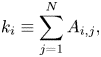 \begin{equation} k_i\equiv\sum_{j=1}^N{A_{i,j}}, \end{equation}
where  $N$ is the total number of nodes, which corresponds to the number of sampled values of the signal (Newman Reference Newman2018). The top panel in figure 2(a) shows the sequence of degree values for the example of signal,
  $s_i$, shown in the bottom of figure 2(a); for instance, the degree of node
  $i=8$ (highlighted in red) is
  $k_8=7$ because it is connected to seven other points (links are highlighted in orange). By averaging over all nodes, a representative degree value for the network (i.e. for the whole signal) is obtained as
  $K=\sum _{i}{k_i}/N$. It should be noted that the degree,
  $k_i$, provides a measure of the extent to which a single node
  $i$ belongs to a convex interval in the signal, but it is not directly able to quantify whether the properties of node
  $i$ (e.g. its importance in the network) are similar or not to the properties of other nodes. Instead, this issue can be tackled through assortativity measures, which can be used to assess similarities among nodes (e.g. in terms of their importance in the network through degree–degree correlation) (Newman Reference Newman2018).
Recalling that long-range links are unlikely to appear in visibility graphs (figure 2b), the main contribution to degree values arises from short-range links, which makes the degree a metric that is typically sensitive to the local structure of the signal. Rapidly fluctuating signals are then expected to show lower-degree values,  $k_i$, and in turn, a lower-average degree
  $K$ (Zhuang et al. Reference Zhuang, Small and Feng2014). Because rapid variations in the local structure of turbulent signals are mainly governed by high frequencies (i.e. low wavelengths), a relation should exist between the average degree,
  $K$, and the high-frequency spectral energy (that produces the local variations in the turbulent signals).
With the aim to explore this relation, we report in figure 3(a) the energy spectral density of the streamwise velocity,  $\phi _{uu}$, pre-multiplied for the wavenumber,
  $\kappa _x=2{\rm \pi} /\lambda _x$, from a turbulent channel flow at
  ${\textit {Re}}_\tau \approx 5200$ (see § 3.1). Notice that
  $\phi _{uu}$ is normalized by the variance of the streamwise velocity fluctuations,
  $\langle uu\rangle _{t,x,z}$ (here angular brackets indicate the average over time,
  $t$, and homogeneous directions,
  $x,z$). In figure 3(a), the spectral peak separation is easily distinguishable between the small and large scales, as is the spectral filter adopted in this work, marked by a horizontal dashed line. Five curves of the spectrum at five representative
  $y^+$ coordinates (highlighted as dashed vertical lines in figure 3a) are also shown in figure 3(b).

Figure 3. (a) Pre-multiplied energy spectral density,  $\phi _{uu}$, from a turbulent channel flow at
  ${\textit {Re}}_\tau \approx 5200$ (see § 3.1), normalized by the streamwise velocity variance,
  $\langle uu\rangle _{t,x,z}$. The horizontal dashed line indicates the value of the spectral filter, while vertical dashed lines highlight five representative
  $y^+$ coordinates. (b) Pre-multiplied energy spectral density for the five selected
  $y^+$ locations in (a). (c) Wall-normal behaviour of the average degree centrality,
  $\langle K\rangle$, for NVG built from the full streamwise velocity,
  $u(x_i)$ (black curve), and from the small-scale streamwise velocity,
  $u_{SS}(x_i)$ (red curve), obtained through a spectral decomposition. Angular brackets in
  $\langle K\rangle$ indicate averaging over the (homogeneous) spanwise direction,
  $z$.
$z$.
The rationale behind the normalization of the spectrum through the variance is twofold. First, the streamwise energy density at each  $y^+$ is accentuated, thus emphasizing the occurrence of the two spectral peaks and, second, this normalization permits a congruent comparison with the degree behaviour computed on visibility networks (which are insensitive to different variance levels, i.e. on signal rescaling). Moreover, as a result of the variance normalization, the area under each curve in figure 3(b) is equal to unity, so that the integral of curves in figure 3(b) in a given range of
  $\lambda _x$ represents the fraction of total energy pertaining to that scale range. In this way, figure 3(b) elucidates the redistribution of the spectral energy density over scales,
  $\lambda _x^+$, at different
  $y^+$ coordinates (a log–log plot in figure 3(b) is shown with the aim to highlight the behaviour at small
  $\lambda _x^+$ values).
Focusing on the small scales (that is,  $\lambda _x^+<{\textit {Re}}_\tau \approx 5200$) in figure 3(b), we observe that by moving from very close to the wall (
 $y^+\approx 0.07$) up to
  $y^+\approx 4$, there is a small decrease in the (normalized) energy content, then an increase of the (normalized) spectral energy occurs from
  $y^+\approx 4$ up to the beginning of the log layer (
 $y^+\approx 50$), and lastly a persistent decrease happens up to the channel centreline (
 $y^+\approx 5200$). A reduction or a growth of the (normalized) spectral energy at the small scales indicates that the signal tends to be locally smoother (i.e. slowly varying, without rapid low-intensity fluctuations) or more irregular (i.e. rapidly varying), respectively. Recalling that the mean degree,
  $K$, is sensitive to the local structure of the signal, an increase of the degree values is then expected for locally smoother signals (i.e. low-spectral energy at local scales) and vice versa. Figure 3(c) shows the wall-normal behaviour of the mean degree,
  $K$, of networks built from the full streamwise velocity,
  $u(x_i)$ (black line), in the channel flow setup. As expected, the
  $y^+$-trend of
  $K$ for the full signal closely follows the behaviour of the small-scale spectral-energy density as described above, where the degree growth is faithfully related to the small-scale spectral-energy decrease and vice versa. In particular, we point out that the value of
  $K$ at each
  $y^+$ is associated to an integral effect of all wavelengths in the signal, so that
  $K(y^+)$ arises from a cumulative effect of different spectral-energy levels.
Figure 3(c) also shows the  $y^+$-behaviour of the mean degree of networks built from
  $u_{SS}(x_i)$ (red line), namely, in which the large-scale component is removed. The values and the trends of
  $K$ from the full and the small-scale velocity signals are very close, and a slight difference appears only very far from the wall. Note that a similar behaviour of
  $K$ as that shown in figure 3(c) for the channel case is also found for the turbulent boundary layer case. It should be noted that because very long-range connections are unlikely to appear (figure 2b), they only barely contribute to the average degree,
  $K$, which instead is mainly related to shorter links.
The excellent agreement between  $K(y^+)$ for the full
  $u$ signal and the
  $y^+$-variations in the small-scale spectral energy (corroborated by the similarity of
  $K(y^+)$ for
  $u$ and
  $u_{SS}$) indicate that the network degree is able to capture the features of the small-scale turbulence directly from the full signal, i.e. without the arbitrary requirements of filtering operations. These features will be exploited in § 2.3 to provide a metric which is able to quantify FM. We notice that, to the best of our knowledge, this is the first time that insights from the visibility graph approach are directly related to the spectral properties of a signal.
2.3. FM detection via degree centrality
The aim of this section is to provide a degree-based metric that is able to quantify FM from full velocity signals. With this aim, in figure 4(b), we show a short representative interval of the streamwise velocity series reported in figure 4(a), which is extracted from the turbulent channel flow at  $y^+\approx 10$. The corresponding NVG is then built from the short signal in figure 4(b), and the links activated by two representative nodes,
  $i=\lbrace 19,49\rbrace$ (highlighted as red dots in figure 4b), are shown as green arcs in figure 4(c). Node
  $i=19$ clearly displays more connections than node
  $i=49$ (i.e.
  $k_{19}>k_{49}$), because node
  $i=19$ is in a larger convex interval than
  $i=49$; therefore, the signal around
  $i=49$ varies more rapidly than around
  $i=19$. Therefore, although the degree,
  $k_i$, represents a pointwise value, because
  $k_i$ refers to a single coordinate
  $i$, the information enclosed in
  $k_i$ originates from the surroundings of
  $i$. The degree
  $k_i$ can then be interpreted as a measure of the instantaneous period (or instantaneous wavelength) at the temporal (or spatial) coordinate
  $t_i$ (or
  $x_i$), by analogy with the concept of instantaneous frequency used in signal analysis (Huang et al. Reference Huang, Shen, Long, Wu, Shih, Zheng, Yen, Tung and Liu1998; Boashash Reference Boashash2015). Larger
  $k_i$ values correspond to larger instantaneous periods (or wavelengths), and, in turn, to smaller instantaneous frequencies.
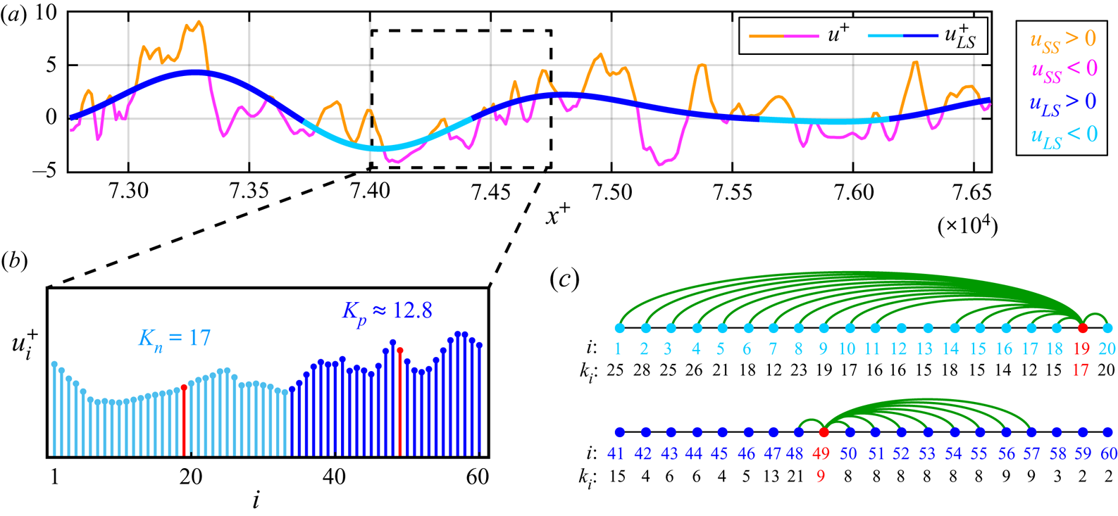
Figure 4. (a) An interval of the streamwise velocity,  $u$, and its large-scale component,
  $u_{LS}$, extracted along the streamwise direction,
  $x$, of the turbulent channel flow at
  $y^+\approx 10$. The full
  $u$ signal is depicted as orange–magenta lines, which indicate intervals of positive and negative small-scale velocity fluctuations,
  $u_{SS}=u-u_{LS}$, respectively, while the
  $u_{LS}$ signal is depicted as light–dark blue lines, which highlight intervals of
  $u_{LS}<0$ and
  $u_{LS}>0$, respectively. Both the series are normalized in wall units. (b) A section consisting of
  $60$ data points of the velocity
  $u$ from (a), depicted as vertical bars whose colour reflects the sign of
  $u_{LS}$. Two representative data points (corresponding to nodes
  $i=19$ and
  $i=49$ of the NVG network) are highlighted in red. (c) Network representation of the NVG built from the signal in (b). Two subsets of nodes and links from the two representative nodes,
  $i=\lbrace 19, 49\rbrace$, are shown as coloured dots and green arcs, respectively. The sequence of degree values,
  $k_i$, for each node,
  $i$, is also reported.
On the basis of this argument and the insights illustrated in § 2.2, we introduce the ratio,  $K_{np}$, to quantify frequency modulation, defined as
 \begin{equation} K_{np}\equiv\frac{K_n}{K_p},\quad K_n=\frac{1}{N_{neg}}\sum_{j=1}^N{(k_j\,|\,u_{LS}<0)},\quad K_p=\frac{1}{N_{pos}}\sum_{j=1}^N{(k_j\,|\,u_{LS}>0)}, \end{equation}
where  $K_n$ and
  $K_p$ are the average degree values computed on the NVG of the full velocity signal, conditioned to intervals of
  $u_{LS}<0$ and
  $u_{LS}>0$, respectively, while
  $N_{neg}$ and
  $N_{pos}$ are the number of occurrences in which
  $u_{LS}<0$ and
  $u_{LS}>0$, respectively.
Values of  $K_{np}$ greater than
  $1$ indicate that the degree is (on average) larger during
  $u_{LS}<0$ intervals than during during
  $u_{LS}>0$, and vice versa for
  $K_{np}$ smaller than
  $1$. In the example of figure 4(b,c), the degree values,
  $k_i$, of the two representative nodes in red (
 $k_{19}=17$ and
  $k_{49}=9$) exemplify the behaviour of the two signal intervals during
  $u_{LS}<0$ and
  $u_{LS}>0$, which result in
  $K_n=17$,
  $K_p\approx 12.8$ and
  $K_{np}>1$. Hence,
  $K_{np}$ discriminates among (i) positive FM for
  $K_{np}>1$ (i.e. an increase of the local frequency in the velocity signal gained for
  $u_{LS}>0$ and a decrease for
  $u_{LS}<0$), (ii) negative FM for
  $K_{np}<1$, and (iii) an absence of modulation for
  $K_{np}\approx 1$. We emphasize that the arguments leading to the ratio (2.3a–c) do not involve any a priori parameters, but only the unique availability of the full velocity signal to compute the degree value of each node. A filtering operation is only required to condition the degree values to the sign of the large-scale velocity.
To test the NVG-based approach, we built synthetic signals that mimic the near-wall modulation mechanism in wall-bounded turbulence for three modulation cases: amplitude modulation (AM), frequency modulation (FM), and both amplitude and frequency modulation (AM+FM). Appendix A contains details on the synthetic signal construction and reports the  $K_{np}$ values for each configuration (see figure 9), which shows that
  $K_{np}$ is able to highlight the presence of FM and, in presence of both AM and FM mechanisms, tends to be more sensitive to FM while only weakly to AM.
In summary, the  $K_{np}$ ratio combines the capability of visibility networks (i) to capture the information on the local temporal structure of a series (§ 2.1), and (ii) to inherit the small-scale energetic features from the full signal (§ 2.2). These characteristics make the visibility approach a powerful and easy-to-use alternative to previously proposed methodologies for time–frequency characterization of turbulence signals. In the following, the NVG approach is carried out for wall-turbulent signals, which reveals its robustness (with respect to different cut-off filtering size) and effectiveness in capturing the large-to-small scale FM mechanism.
3. Description of the turbulent flow datasets
Two main datasets of high-Reynolds-number wall-bounded turbulent flows are exploited in this work to study FM by means of visibility-network-based tools: (i) spatial series from a numerically-simulated turbulent channel flow at  ${\textit {Re}}_\tau \approx 5200$ (Lee & Moser Reference Lee and Moser2015); and (ii) time series from experimental measurements in a turbulent boundary layer at
  ${\textit {Re}}_\tau =14\,750$ (Marusic Reference Marusic2020). Although outer flow structures start to occur and play a role in scale interaction at lower Reynolds numbers (Agostini & Leschziner Reference Agostini and Leschziner2014; Hu & Zheng Reference Hu and Zheng2018; Wu et al. Reference Wu, Christensen and Pantano2019), high-Reynolds-number flows are required to enhance the inter-scale separation and amplify the scale interaction mechanism. Moreover, a third DNS dataset of turbulent channel flow at
  ${\textit {Re}}_\tau =1000$ is also employed for comparison purposes, thus showing effects of inertia on FM results.
To the best of our knowledge, this is the first time a state-of-the-art DNS at  ${\textit {Re}}_\tau \approx 5200$ is employed to specifically investigate large-to-small scale FM. In fact, while high-Reynolds-number boundary-layer flows are typically obtained in experimental facilities (as witnessed by most previous works on AM and FM), high-
 ${\textit {Re}}_\tau$ experiments of channel flows are difficult to realise owing to strong side-wall boundary effects (Lee & Moser Reference Lee and Moser2015). The DNS employed in this work is at a sufficiently large Reynolds number (i.e.
  ${\textit {Re}}_\tau >4000$, as reported by Hutchins & Marusic Reference Hutchins and Marusic2007b) to guarantee a sufficient large–small-scale spectral separation (e.g. see energy peaks separation in figure 3a), and allows us to perform a FM analysis on all the three velocity components that, so far, has only been performed for AM (e.g. see Talluru et al. Reference Talluru, Baidya, Hutchins and Marusic2014; Agostini & Leschziner Reference Agostini and Leschziner2016).
The scale decomposition of the streamwise velocity fluctuation signals was performed as  $u(x)=u_{LS}(x)+u_{SS}(x)$ (e.g. figure 4a) and
  $u(t)=u_{LS}(t)+u_{SS}(t)$ (e.g. figure 1b) for the spatial and time series taken from the turbulent channel and boundary layer flows, respectively. A common approach to obtain
  $u_{SS}$ and
  $u_{LS}$ is to employ a spectral filter to retain the high and low wavelength or frequency, respectively, as performed in several previous works (Mathis et al. Reference Mathis, Hutchins and Marusic2009a; Ganapathisubramani et al. Reference Ganapathisubramani, Hutchins, Monty, Chung and Marusic2012; Baars et al. Reference Baars, Talluru, Hutchins and Marusic2015, Reference Baars, Hutchins and Marusic2017; Pathikonda & Christensen Reference Pathikonda and Christensen2017, Reference Pathikonda and Christensen2019). Alternatively, Agostini & Leschziner (Reference Agostini and Leschziner2014) proposed employing empirical mode decomposition (Huang et al. Reference Huang, Shen, Long, Wu, Shih, Zheng, Yen, Tung and Liu1998) to separate the large- and small-scale contributions. In this work, both the spectral and empirical mode decompositions were tested to separate the large- and small-scale contributions. However, for the sake of simplicity and in line with most of the current literature, results are only shown for a spectral decomposition, as both the procedures produce equivalent results.
3.1. DNS of turbulent channel flows
Velocity fields were extracted from two direct numerical simulations of incompressible turbulent channel flows. The first DNS was run at frictional Reynolds number  ${\textit {Re}}_\tau \equiv h U_\tau /\nu =5186$, where
  $h=1$ is the half-channel height,
  $U_\tau =4.14872\times 10^{-2} U_b$ and
  $\nu =8\times 10^{-6} U_b h$, with the bulk velocity
  $U_b=1$. The size of the spatial domain was
  $(8{\rm \pi} h \times 2h \times 3{\rm \pi} h)$ with
  $(10\,240 \times 1536 \times 7680)$ grid points along the streamwise, wall-normal and spanwise directions, respectively. The flow fields were recorded only after statistical stationarity of the flow was reached, and
  $11$ temporal frames of the velocity and pressure spatial fields were stored in the dataset. The time interval between two consecutive frames was a flow-through time of approximately
  $0.7$, which corresponded to approximately
  $3785\nu /U_\tau ^2$ in wall units.
The simulation was performed at a sufficiently high Reynolds number and with a sufficiently large spatial domain to exhibit characteristics of high-Reynolds-number turbulence, e.g. the presence of LSMs and a rather large wall-normal range for statistics scaling (Lee & Moser Reference Lee and Moser2015). The dataset is available online (doi:10.7281/T1PV6HJV) from the Johns Hopkins Turbulence Database (Li et al. Reference Li, Perlman, Wan, Yang, Meneveau, Burns, Chen, Szalay and Eyink2008). For further simulation details and statistics, see Lee & Moser (Reference Lee and Moser2015).
The second DNS was run at  ${\textit {Re}}_\tau \equiv h U_\tau /\nu =1000$, with
  $h=1$,
  $U_\tau =4.9968\times 10^{-2} U_b$,
  $\nu =5\times 10^{-5} U_b h$ and
  $U_b=1$. The size of the spatial domain was
  $(8{\rm \pi} h \times 2h \times 3{\rm \pi} h)$ with
  $(2048 \times 512 \times 1536)$ grid points along the streamwise, wall-normal and spanwise directions, respectively. Data were stored for approximately one flow-through time,
  $[0,26]h/U_b$, with a storage temporal step of
  $0.0065$. This dataset is also available online (doi:10.7281/T10K26QW) from the Johns Hopkins Turbulence Database (Li et al. Reference Li, Perlman, Wan, Yang, Meneveau, Burns, Chen, Szalay and Eyink2008). For further simulation details, see Graham et al. (Reference Graham2016).
In this work, 1-D spatial series (i.e. extracted at a fixed time) of the three velocity components,  $u,v,w$, along the streamwise direction,
  $x$, were exploited to build visibility networks. Network-based results were averaged in time (i.e. on
  $11$ temporal frames for the
  ${\textit {Re}}_\tau \approx 5200$ set-up, and on
  $400$ uniformly-spaced temporal frames for the
  ${\textit {Re}}_\tau = 1000$ set-up) and in the spanwise direction; in the latter case, averages were performed for a set of uniformly-spaced spanwise locations separated from each other by
  $64$ and
  $128$ grid points for the
  ${\textit {Re}}_\tau \approx 5200$ and
  ${\textit {Re}}_\tau =1000$ configurations, respectively.
The cut-off spectral filter to separate the large- and small-scale streamwise velocity for the  ${\textit {Re}}_\tau \approx 5200$ set-up was set equal to
  $\lambda _{x,c}=h$ (i.e.
  $\lambda _{x,c}^+=5186$), in analogy with previous works in which
  $\lambda _{x,c}$ was set equal to the boundary layer thickness (Hutchins & Marusic Reference Hutchins and Marusic2007b; Mathis et al. Reference Mathis, Hutchins and Marusic2009a,Reference Mathis, Monty, Hutchins and Marusicb; Marusic et al. Reference Marusic, Mathis and Hutchins2010; Dogan et al. Reference Dogan, Örlü, Gatti, Vinuesa and Schlatter2019; Wu et al. Reference Wu, Christensen and Pantano2019). For the
  ${\textit {Re}}_\tau =1000$ set-up, the cut-off filter was
  $\lambda _{x,c}^+=5000$, thus was comparable to
  $\lambda _{x,c}^+$ of the higher-
 ${\textit {Re}}_\tau$ channel flow set-up.
3.2. Experimental turbulent boundary layer at  ${\textit {Re}}_\tau \approx 14\,750$

Experimental measurements were performed in the wind-tunnel facility of the University of Melbourne, which employs a  $27\ \mathrm {m}$ test section, under a free-stream velocity
  $U_\infty =19.95\ \mathrm {m}\ \mathrm {s}^{-1}$ (Baars et al. Reference Baars, Talluru, Hutchins and Marusic2015). Under these conditions, a zero-pressure-gradient boundary layer developed at a frictional Reynolds number
  ${\textit {Re}}_\tau \equiv \delta U_\tau /\nu =14\,750$, where
  $\delta =0.361\ \mathrm {m}$ is the boundary layer thickness at the measuring location (i.e.
  $21.65\ \mathrm {m}$ from the inlet of the test section), while
  $U_\tau =0.626\ \mathrm {m}\ \mathrm {s}^{-1}$ and
  $\nu =1.532\times 10^{-5}\ \mathrm {m}^2\ \mathrm {s}^{-1}$ at the same streamwise location. The dataset was the same employed by Baars et al. (Reference Baars, Talluru, Hutchins and Marusic2015, Reference Baars, Hutchins and Marusic2017), and is available online at the Fluid Mechanics Research webpage of the University of Melbourne (Marusic Reference Marusic2020).
Time series of the streamwise velocity were simultaneously recorded by means of two constant-temperature hot-wire probes, one at a fixed wall-normal location at  $y^+=4.33$, and the other vertically moved throughout the boundary layer in the range
  $y^+\in [10.5,2.14\times 10^4]$ (or
  $y/\delta \in [7.087\times 10^{-4},1.45]$) for
  $40$ vertical locations. At each wall-normal measurement location, three sets of data were recorded at a sampling frequency of
  $20\ \mathrm {kHz}$, each one for
  $120\ \mathrm {s}$ corresponding to a large-scale time of
  $6.6\times 10^3\delta /U_\infty$, thus ensuring the convergence of spectral statistics at the longest energetic wavelengths (Baars et al. Reference Baars, Talluru, Hutchins and Marusic2015). The resulting time step in wall units was
  ${\rm \Delta} t^+=1.28$. Further details on the measurement procedure and instrumentation can be found in Baars et al. (Reference Baars, Talluru, Hutchins and Marusic2015).
To separate the large- and small-scale components, we employed a cut-off spectral filter  $\lambda _{x,c}^+=7000$ following Hutchins & Marusic (Reference Hutchins and Marusic2007b), Hutchins (Reference Hutchins2014) and Baars et al. (Reference Baars, Talluru, Hutchins and Marusic2015, Reference Baars, Hutchins and Marusic2017), who showed this is a proper filter value for turbulent boundary layers at high Reynolds numbers. Differently from the channel flow set-up in which spatial series are considered, here the spectral filter was converted in terms of frequency by invoking the Taylor's hypothesis as
  $f_c(y^+)=U_c(y^+)/\lambda _{x,c}$, where
  $U_c(y^+)$ is a local convection velocity at the wall-normal coordinate
  $y^+$. The effects of different convection velocities on FM will be elucidated in § 4, where a comparison with spatial data from DNSs is carried out.
4. Results
The results from the application of the degree centrality as a metric to quantify frequency modulation are reported in this section for velocity signals extracted from the turbulent channel flows and the turbulent boundary layer described above. A one-point modulation analysis was carried out: the large scale component,  $u_{LS}$, used to condition the degree on the
  $u_{LS}$ sign (see (2.3a–c)) was extracted at the same
  $y^+$ in which the signal was mapped into a visibility network. Owing to the footprint of the LSMs and VLSMs towards the wall,
  $u_{LS}$ evaluated at each
  $y^+$ represented a good estimate of the large-scale velocity component in the outer region, thus resulting in a more applicable procedure than the two-points analysis (Mathis et al. Reference Mathis, Hutchins and Marusic2009a). In fact, two-point synchronized measurements are not easy to perform experimentally (Mathis et al. Reference Mathis, Hutchins and Marusic2009a). Previous works have shown that similar results are obtained by adopting a one- or two-point procedure for characterizing scales interaction (see, among others, Hutchins & Marusic (Reference Hutchins and Marusic2007a); Mathis et al. (Reference Mathis, Hutchins and Marusic2009a); Ganapathisubramani et al. (Reference Ganapathisubramani, Hutchins, Monty, Chung and Marusic2012)), thus one-point modulation was preferred here for simplicity.
First, the streamwise velocity component,  $u$, was considered, both in an overall perspective (§ 4.1) and with a near-wall focus (§ 4.2). Most of the current literature on scale interaction in wall-bounded turbulence has indeed focused on the
  $u$ component, being the component in which the large and small scales can be clearly separated. We then extended the analysis to the other velocity components,
  $v$ and
  $w$ (§ 4.3). Finally, a space-shifted FM analysis was carried out for all velocity components and for both the turbulence configurations (§ 4.4).
4.1. FM in the streamwise velocity component
The values of the ratio  $K_{np}$ as a function of the wall-normal coordinate,
  $y^+$, are shown in figure 5 for visibility networks built from the streamwise velocity,
  $u$. We recall that
  $K_{np}>1$ indicates a higher frequency under intervals of positive large-scale velocity than under negative ones, and vice versa for
  $K_{np}<1$.
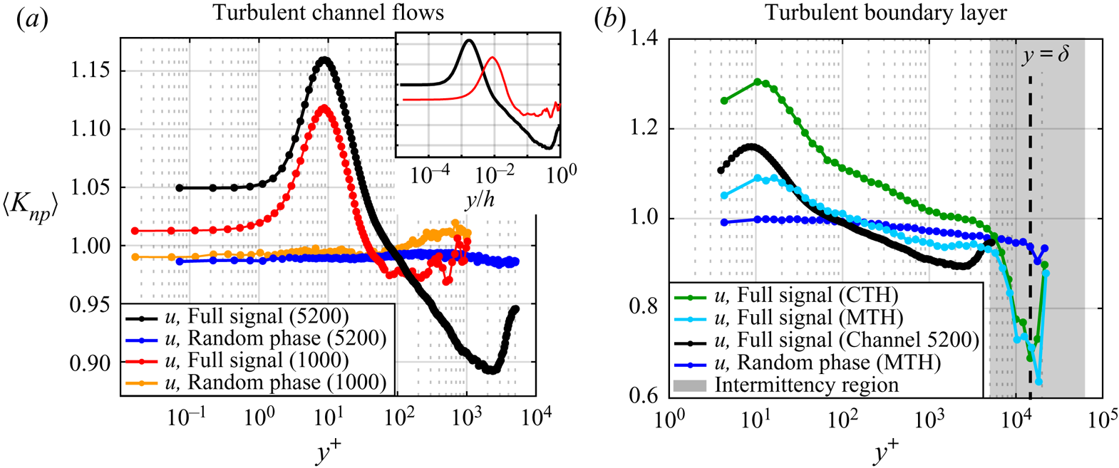
Figure 5. Large-scale conditional average degree ratio,  $K_{np}$, as a function of the wall-normal coordinate,
  $y^+$, for streamwise velocity,
  $u$, extracted from (a) the channel flow DNS at different
  ${\textit {Re}}_\tau$ and (b) the boundary layer experiment. The inset in (a) shows the
  $K_{np}$ behaviour for the two channel flows as a function of
  $y/h$. In (b),
  $K_{np}(y^+)$ is shown for the spatial series obtained through the classical (CTH) and modified Taylor's hypothesis (MTH) as green and cyan plots, respectively; for comparison, the behaviour for the channel flow at
  ${\textit {Re}}_\tau \approx 5200$ is also reported in black. Moreover, the boundary layer intermittency region is highlighted in (b) as a shaded grey region. Angular brackets indicate averaging over time and spanwise direction in (a) and over three different realizations in (b). The results for synthetic velocity signals with shuffled phases are also shown.
Figure 5(a) shows  $K_{np}$ for the spatial series of the two channel flows DNS at
  ${\textit {Re}}_\tau \approx 5200$ (black) and
  ${\textit {Re}}_\tau =1000$ (red), while figure 5(b) illustrates the
  $K_{np}$ behaviour for the time series of the boundary layer (green). Values of
  $K_{np}>1$ were detected close to the wall for all configurations, while moving away from the wall,
  $K_{np}$ became smaller than
  $1$, which indicated a reversal in the scale-interaction mechanism, i.e. higher frequencies were detected during
  $u_{LS}<0$ than for
  $u_{LS}>0$. The overall behaviours shown in figure 5 were in accordance with previous works on scale interaction in wall-bounded turbulence, which have indicated that a higher (amplitude and) frequency of the small scales is found for positive
  $u_{LS}$ intervals in regions close to the wall, while a reversal mechanism occurs far from the wall (Ganapathisubramani et al. Reference Ganapathisubramani, Hutchins, Monty, Chung and Marusic2012; Baars et al. Reference Baars, Talluru, Hutchins and Marusic2015, Reference Baars, Hutchins and Marusic2017; Pathikonda & Christensen Reference Pathikonda and Christensen2017; Awasthi & Anderson Reference Awasthi and Anderson2018; Tang & Jiang Reference Tang and Jiang2018; Pathikonda & Christensen Reference Pathikonda and Christensen2019). However, the behaviour of
  $K_{np}(y^+)$ for the two set-ups also highlights peculiar features of large-to-small scale FM that deserve further investigations.
First, we compared the results for the two channel flows at different Reynolds numbers (red and black lines in figure 5a). A similar trend of  $K_{np}(y^+)$ was found for both channels, but the intensity of the FM (close to the wall) was larger for
  ${\textit {Re}}_\tau \approx 5200$ than for
  ${\textit {Re}}_\tau =1000$, thus clearly showing that the effect of higher Reynolds numbers was to increase the FM mechanism in the near-wall region, as a consequence of the increasing magnitude of the large-scale fluctuations with increasing
  ${\textit {Re}}_\tau$. Similarly, away from the wall, the reversal mechanism of scale interaction was strengthened for the higher-Reynolds-number DNS. Furthermore, in figure 5(a) and also in figure 5(b) for the boundary layer, we observed a peak of
  $K_{np}$ at
  $y^+\approx 10$: this peak was shown to be related to strong sweep-like events, a phenomenon referred to as ‘splatting’ in which the large scales transport the high-intensity small scales towards the wall below the buffer layer (Agostini & Leschziner Reference Agostini and Leschziner2014; Agostini et al. Reference Agostini, Leschziner and Gaitonde2016). Thus, being the highest small-scale intensity detected in the buffer layer (Agostini et al. Reference Agostini, Leschziner and Gaitonde2016), the strongest FM is revealed by a peak in
  $K_{np}$, which then represents a sensitive metric to local changes in the flow dynamics. Eventually, it was remarkable to observe in figure 5(a) the near-wall agreement of
  $K_{np}$ plotted against
  $y^+$ between the two channel flows at different Reynolds numbers, as the near-wall dynamics is related to near-wall cycle whose characteristic scales are fixed in wall units (see also a discussion on characteristic near-wall spatial and temporal scales in § 4.4).
The behaviour of  $K_{np}$ obtained from the time series of the turbulent boundary layer is shown in figure 5(b). When time series are considered, a convection velocity,
  $U_c$, has to be defined to apply Taylor's hypothesis in filtering the large and small scales. Typically,
  $U_c$ is set equal to the local mean velocity,
  $U$, and in the following, this assumption will be referred to as the CTH. Here,
  $K_{np}$ obtained through the CTH is displayed as a function of
  $y^+$ in green in figure 5(b); although a similar behaviour with respect to the channel flows is observed (e.g. the black line in figure 5b), there is a significant vertical shift when time series are employed. It is worth noting that, because the local mean velocity,
  $U$, does not depend on time, the temporal structure of the time series is preserved when the CTH is applied. This implies that the application of any technique (including NVG) to study the scale interaction from a time series is the same as from the corresponding spatial series (i.e. obtained through the CTH), because
  ${\rm \Delta} x\propto {\rm \Delta} t$.
The overestimation of modulation parameters when the time series and CTH are used has been previously observed for AM in jet (Fiscaletti et al. Reference Fiscaletti, Ganapathisubramani and Elsinga2015), mixing layer (Fiscaletti et al. Reference Fiscaletti, Attili, Bisetti and Elsinga2016) and turbulent boundary layer flows (Yang & Howland Reference Yang and Howland2018). Specifically, Yang & Howland (Reference Yang and Howland2018) reported a distortion of the spatial series when the CTH is used and suggested employing a convection velocity,  $U_c$, defined as
  $U_c(t)=U+\alpha u(t)$, where
  $u(t)=u_{LS}(t)+u_{SS}(t)$ is the fluctuating component of the streamwise velocity and
  $\alpha =O(1)$ is a proportionality constant. The correction proposed by Yang & Howland (Reference Yang and Howland2018) is based on the rationale that the sampling time step has to be scaled using the local viscous scales, so that the small-scale activity is enhanced (or reduced) where the wall shear stress is high (or low) owing to an increase (decrease) in the local friction velocity (Yang & Howland Reference Yang and Howland2018). However, variations in the (fluctuating) wall shear stress are mainly induced by variations into large-scale fluctuations,
  $u_{LS}(t)$, rather than
  $u(t)$, as observed by Yang & Howland (Reference Yang and Howland2018) and reported in the previous literature (e.g. Zhang & Chernyshenko Reference Zhang and Chernyshenko2016; Baars et al. Reference Baars, Hutchins and Marusic2017) (see a more detailed discussion about the relation between the near-wall small scales and wall shear stress in § 4.2). Therefore, in this work, we exploited the time varying formulation by Yang & Howland (Reference Yang and Howland2018) but only accounted for the large-scale component of
  $u(t)$, namely
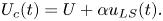 \begin{equation} U_c(t)=U+\alpha u_{LS}(t). \end{equation}
In what follows, we will refer to the application of (4.1) as the convection velocity as the MTH, where we selected  $\alpha =0.8$ (which has been proven to be a suitable value). It should be noted that a correction based on
  $u_{LS}$ arguments was also discussed by Fiscaletti et al. (Reference Fiscaletti, Ganapathisubramani and Elsinga2015) for jet and boundary layer flows to compensate for an AM overestimation. Moreover, it should be noted that, different form the CTH, the structure of
  $u(x)$ is different from the structure of
  $u(t)$ for the MTH case, because
  $U_c(t)$ is not a constant, thus leading to a non-uniform spacing of the spatial series.
The  $K_{np}$ behaviour for the MTH is shown in cyan in figure 5(b): the overestimation of
  $K_{np}$ is compensated and its values are much more comparable to the spatial series obtained from DNS of the channel flow at
  ${\textit {Re}}_\tau \approx 5200$ (black line in figure 5b). This analysis confirms the applicability of the time-dependent correction of Yang & Howland (Reference Yang and Howland2018) for AM when time series are employed, and extends such a correction to the study of FM through (4.1). In particular, we stress that
  $u_{LS}(t)$ represents a more suitable choice than
  $u(t)$ in (4.1) because it is assumed that fluctuations in the large-scale velocity,
  $u_{LS}(t)$, drive the variations in the friction velocity affecting the behaviour of the small scales (see relation (4.2) and the accompanying discussion). In this regard, the relation (4.1) leads to scaling arguments that are in good agreement with the quasi-steady quasi-homogeneous theory, as will be discussed in § 4.2.
One additional feature emerging from figure 5 concerns the reversal in the modulation mechanism from the wall proximity to the outer flow. In fact, while figure 5 shows a continuous decrease of  $K_{np}$ for
  $y^+>10$ and
  $y/h \lesssim 0.5$, an almost absence of FM was previously found in the log region by means of other techniques (where a reversal of the FM was only detected in the proximity of the end of the boundary layer) (Ganapathisubramani et al. Reference Ganapathisubramani, Hutchins, Monty, Chung and Marusic2012; Baars et al. Reference Baars, Talluru, Hutchins and Marusic2015). We point out that the
  $K_{np}$ behaviour in figure 5 resembles the decreasing behaviour of the AM parameters (e.g. see Mathis et al. Reference Mathis, Hutchins and Marusic2009a,Reference Mathis, Monty, Hutchins and Marusicb), with a reversal of
  $K_{np}$ from the near-wall (where
  $K_{np}>1$) towards the outer region (where
  $K_{np}<1$). In principle, if the small scales are both amplitude and frequency modulated, one could expect that – following the Newtonian principle that to the same natural effects we must, as far as possible, assign the same causes – a similar underlying mechanism is at play for both AM and FM. This can justify the similarity between the
  $K_{np}(y^+)$ behaviour, which quantifies FM, and the widely reported behaviour of AM parameters, either in internal or external wall-bounded turbulent flows. Therefore, both AM and FM result from a common underlying phenomenon, for which both the amplitude and frequency of the small scales are concurrently affected by negative or positive large-scale fluctuations at different wall-normal locations.
Specifically, concerning the reversal coordinate (i.e. the  $y^+$ location where
  $K_{np}$ switches from
  $K_{np}>1$ to
  $K_{np}<1$), for AM, the reversal typically occurs in the middle of the log region,
  $y^+\approx 3.9 {\textit {Re}}_\tau ^{1/2}$ (Mathis et al. Reference Mathis, Hutchins and Marusic2009a,Reference Mathis, Monty, Hutchins and Marusicb; Ganapathisubramani et al. Reference Ganapathisubramani, Hutchins, Monty, Chung and Marusic2012; Baars et al. Reference Baars, Talluru, Hutchins and Marusic2015). For FM, it is still not clear whether a modulation reversal occurs in the log region (as shown in figure 5) or if it is only limited to the wake region (Baars et al. Reference Baars, Talluru, Hutchins and Marusic2015). From figure 5, we can conclude that the FM mechanism is indeed limited to a near-wall region up to approximatively
  $y^+= 100$, which is consistent with the analysis by Ganapathisubramani et al. (Reference Ganapathisubramani, Hutchins, Monty, Chung and Marusic2012). Nevertheless, figure 5 also shows that the reversal
  $y^+$ location increases with the Reynolds number. In fact, we find that when the spatial series are focused both from channel DNSs and the time series by the MTH, the reversal coordinates (i.e.
  $y^+\approx 35, 75, 145$ for the channel and boundary layer flows at
  ${\textit {Re}}_\tau =1000, 5186, 14\,750$, respectively) scale as
  $y^+\approx 1.15{\textit {Re}}_\tau ^{1/2}$ (the power-law fit gives an exponent of
  $0.5$ with an
  $R^2=0.985$). This scaling has the same functional relationship found for AM, i.e.
  $y^+\approx 3.9 {\textit {Re}}_\tau ^{1/2}$, but with a different proportionality constant. In particular, the
  ${\textit {Re}}_\tau ^{1/2}$ trend is reminiscent of the scaling of the outer peak position as a function of Reynolds number (Mathis et al. Reference Mathis, Hutchins and Marusic2009a), thus strengthening the underlying connection of FM with the change in large-scale features.
Another notable aspect discernible in figure 5 is the V-like shape of  $K_{np}$ in the outer region of the channel flow, i.e. around
  $y/h\approx 0.5$ (
 $y^+\approx 2500$). In the literature, the increase, which gives the V-like shape, of AM of the small scales (which are representative of fine-scale turbulent motion) can be observed close to the channel centre, e.g. in Chung & McKeon (Reference Chung and McKeon2010) (see figure 4 therein) for the streamwise velocity,
  $u$, or in Yao et al. (Reference Yao, Huang and Xu2018) (see figure 3(c) therein) for the
  $v$ and
  $w$ components. However, to the best of our knowledge, this peculiar increase of the modulation parameter in the channel flow has not been explicitly discussed so far. Here we propose an interpretation based on the insights gained from turbulent boundary layers.
Previous analyses, in fact, have highlighted that the preferential arrangement of the small scales in the wake region of turbulent boundary layers is mainly affected by intermittency, namely the presence of bulges of turbulent and non-turbulent flow (Baars et al. Reference Baars, Talluru, Hutchins and Marusic2015, Reference Baars, Hutchins and Marusic2017). However, figure 5(a) shows a similar V-like behaviour – as for previous results on AM – also in the outer region of the channel flows, despite the absence of a turbulent/non-turbulent region in the channel flow (that is, an internal flow). In particular, the V-like shape for the channel at  ${\textit {Re}}_\tau =1000$, although less evident than at
  ${\textit {Re}}_\tau \approx 5200$, consistently occurs at
  $y/h\approx 0.5$, as highlighted in the inset of figure 5(a). Here we suggest that, similar to the effect of intermittency in boundary layer flows, the preferential arrangement in the proximity of the channel centreline could be affected by an alternating occurrence of high- and low-rotational fluid motion above the head of large- or very-large-scale structures. This phenomenon would lead to the increase of both the AM and FM parameters toward the channel centreline. Although the clarification of this issue goes beyond the aim of this work, we do believe it deserves future investigations, as the channel flow set-up is much less considered for scale interaction analyses than the turbulent boundary layers (for which high
  ${\textit {Re}}_\tau$ data are much more readily available from experimental measurements).
With the aim to ensure that the behaviour of  $K_{np}(y^+)$ described so far is the result of an intrinsic flow phenomenon, rather than an artefact arising from the network representation, figure 5 shows the results for random-phase signals. Through a randomization of the phase of velocity Fourier coefficients, the energy spectral density and the turbulence intensity do not change, but all phase information is lost. Hence, following Mathis et al. (Reference Mathis, Hutchins and Marusic2009a), first the signals of
  $u$ were phase-scrambled, then the large-scale component,
  $u_{LS}$, was extracted from the new random-phase signal (the amplitude spectrum was not changed), and eventually the degree was calculated from the full random-phase signal and conditioned to the sign of the random-phase
  $u_{LS}$. Figure 5 shows that in both the channel flow and boundary layer set-ups, the characteristic behaviour of
  $K_{np}$ for turbulent signals (black curves) disappeared for the random-phase velocity signals (blue curves). As previously reported (e.g. see Chung & McKeon Reference Chung and McKeon2010), phase relationships between the large and small scales play an important role in the characterization of scale interaction, specifically on scale modulation; thus, if any realistic phase information is lost, modulation effects will disappear as well.
The NVG-based approach is demonstrated to be reliable in capturing FM in turbulent velocity signals, and sensitive to phase randomization. Moreover, the behaviour of  $K_{np}(y^+)$ for both the channel and boundary layer is found to be robust under different cut-off wavelengths (used to extract
  $u_{LS}$ from the full signal
  $u$), as discussed in Appendix B. Further insights into the FM of the streamwise velocity will be presented in § 4.2 focusing on the near-wall region, i.e. where large-to-small scale modulation essentially takes place.
4.2. Scale interaction in the near-wall region
The presence of a near-wall modulation, whose intensity increases with the Reynolds number, has posed a challenge to the classical view on the universality of near-wall turbulence, i.e. the independence of the near-wall statistics (scaled in wall units) to the Reynolds number when this is sufficiently large. Because large-scale structures affect the behaviour of the wall shear stress (Mathis et al. Reference Mathis, Marusic, Chernyshenko and Hutchins2013), the classical universality hypothesis has been recently replaced with the hypothesis that statistics have to be normalized by considering the large-scale skin friction,  $\tau _{LS}$, rather than the mean skin friction,
  $\tau _w$ (Zhang & Chernyshenko Reference Zhang and Chernyshenko2016; Chernyshenko Reference Chernyshenko2020). This hypothesis is referred to as the quasi-steady quasi-homogeneous (QSQH) hypothesis, because the temporal and spatial variations of the large-scale structures are much slower than variations of the near-wall turbulence (Zhang & Chernyshenko Reference Zhang and Chernyshenko2016).
The aim of this section is (i) to provide the proportionality relationships between  $u_{LS}$ and the (temporal or spatial) frequency of the small scales as expected from the QSQH hypothesis; and (ii) to test the validity of such relationships by means of the network degree centrality. In particular, we will focus on velocity signals extracted at
  $y^+=15$, which corresponds to the
  $y^+$ value of maximum
  $K_{np}$ in figure 5, thus being a representative wall-normal coordinate of the near-wall region. This choice is also related to the fact that, evidenced by Zhang & Chernyshenko (Reference Zhang and Chernyshenko2016) and Agostini & Leschziner (Reference Agostini and Leschziner2019), the validity of the QSQH hypothesis is found to be rather accurate only in a narrow region close to the wall, that is,
  $y^+<70-80$.
According to the QSQH hypothesis, variations in the large-scale velocity,  $u_{LS}$, induce proportional variations in the large-scale skin friction,
  $\tau _{LS}$, namely
  $(\tau _w+\tau _{LS}) \propto (U+u_{LS})$, where
  $U$ is the local mean velocity. Because, by definition,
  $U_\tau =\sqrt {\tau _w/\rho }$ (where
  $\rho$ is the fluid density), the effect of
  $u_{LS}$ on
  $\tau _{LS}$ can be stated in terms of velocities as
 \begin{equation} (U_\tau+u_{\tau,LS})\propto \sqrt{(\tau_w+\tau_{LS})} \propto \sqrt{(U+u_{LS})}, \end{equation}
where  $u_{\tau ,LS}$ is the fluctuating (i.e. zero-mean) large-scale component of the friction velocity (Baars et al. Reference Baars, Hutchins and Marusic2017). Owing to near-wall modulation, a quasi-steady or quasi-homogeneous variation of the friction velocity affects also the (amplitude and) frequency of the small scales. Specifically,
  $u_{LS}>0$ events induce
  $u_{\tau ,LS}>0$ (see relation (4.2)) that, in turn, produces an increase of the small-scale instantaneous spatial or temporal frequency according to the FM mechanism; and vice versa for
  $u_{LS}<0$ (Baars et al. Reference Baars, Hutchins and Marusic2017).
In the near-wall region, the spatial scales are supposed to have a constant characteristic length when normalized in wall units (e.g. see the inner spectral peak for  $\lambda _x^+=\lambda _x U_\tau /\nu ={\rm const.}\approx 1000$ in figure 3a). Therefore, spatial scales are related to
  $u_{\tau ,LS}$ variations as
  $\lambda _x (U_\tau +u_{\tau ,LS})={\rm const.}$, namely
  $\lambda _x\propto 1/(U_\tau +u_{\tau ,LS})$. Because the spatial frequency (i.e. wavenumber),
  $\kappa _x$, is related to the spatial scales as
  $\kappa _x\propto \lambda _x^{-1}$, by using (4.2), we obtain the following scaling relations:
 \begin{equation} \lambda_x\propto {(U+u_{LS})}^{{-}1/2},\quad \kappa_x\propto {(U+u_{LS})}^{1/2}. \end{equation}
In the case of a time series, the temporal frequency,  $f$, is related to the spatial scales as
  $f=U_c/\lambda _x$, where
  $U_c$ is the convection velocity. Assuming that
  $U_c$ scales in wall units (Baars et al. Reference Baars, Hutchins and Marusic2017), namely
  $U_c\propto (U_\tau +u_{\tau ,LS})$, the temporal frequency is eventually expected to scale as
 \begin{equation} f\propto (U_\tau+u_{\tau,LS})^2\propto (U+u_{LS}). \end{equation}
Therefore, the relations (4.3a,b) and (4.4) represent the expected scaling of the spatial and temporal frequency, respectively, according to the QSQH hypothesis.
As discussed in § 2.3, the degree centrality represents a measure of the instantaneous wavelength or a temporal period. Therefore, it is expected that the degree,  $k$, scales as
  $k\propto \lambda _x$ for the channel flow (in which spatial series are mapped into NVGs), and
  $k\propto 1/f$ for the boundary layer (in which time series are analysed). If the degree is indeed an effective parameter to quantify FM,
  $k$ should then be proportional to
  $(U+u_{LS})^{\beta _{u,x}}$ in the channel flow and
  $(U+u_{LS})^{\beta _{u,f}}$ in the boundary layer. Following the aforementioned scaling arguments (i.e. relations (4.3a,b) and (4.4)), the two exponents that verify the QSQH hypothesis should be equal to
  $\beta _{u,x}=-0.5$ and
  $\beta _{u,f}=-1$.
To test the  $\beta _{u,x}$ and
  $\beta _{u,f}$ scaling, we conditionally averaged the degree centrality values (computed from NVGs of the full velocity signals
  $u(x)$) to the
  $u_{LS}$ values at
  $y^+\approx 10$. In particular, the
  $u_{LS}$ values were first divided into uniformly-binned intervals in the range between
  $min[u_{LS}] \hbox{ and } max[u_{LS}]$. Then, for each visibility network (i.e. each signal), nodes
  $i$, for which
  $u_{LS}(i)$ belongs to a specific bin, were selected, and the corresponding degree values,
  $k_i$, were averaged for that specific bin. By extending the averages to all
  $u_{LS}$ bins, the conditional average,
  $(\bar {k}\,|\,u_{LS})$, was obtained, where the overbar indicates an average over a set of nodes. When plotting
  $(\bar {k}\,|\,u_{LS})$, the
  $u_{LS}$ value representative of each bin was chosen as the middle value of the bin.
The behaviour of  $(\bar {k}\,|\,u_{LS})$ as a function of
  $u_{LS}$ revealed the scaling between degree-based frequency variations and large-scale velocity variations. Such conditional degree averages are shown in figure 6 for the channel flow at
  ${\textit {Re}}_\tau \approx 5200$ (figure 6a) and the boundary layer (figure 6b), as a function of
  $(u_{LS}/U+1)$, where
  $U=U(y^+=10)$ is constant and
  $(u_{LS}/U+1)$ values equal to
  $1$ correspond to large-scale zero-crossing points (
 $u_{LS}=0$). We find a scaling of the conditioned degree, which follows a power-law with the best-fit exponent
  $\beta _{u,x}=-0.48$ for the channel flow (spatial data) and
  $\beta _{u,f}=-1$ for the boundary layer when the local mean velocity is used in the Taylor's hypothesis (CTH). These exponent values are in excellent agreement with the expected values of
  $-0.5$ and
  $-1$. We recall that, for the CTH case, because the convection velocity is constant and equal to the local mean velocity
  $U$, the scaling exponent obtained is representative of a (temporal) frequency, thus
  $\beta _{u,f}=-1$. However, when the MTH is employed (4.1), the structure of the spatial series (obtained from the corresponding time series) significantly changes and scaling arguments are therefore congruent with the DNS spatial series. Accordingly, the
  $(\bar {k}\,|\,u_{LS})$ scaling for the MTH case in figure 6(b) produces an exponent which is close to
  $-0.5$, as expected from the spatial series. Finally, we mention that an exponent
  $\beta _{u,x}=-0.5$ is found for the channel flow at
  ${\textit {Re}}_\tau = 1000$ with an
  $R^2\approx 0.92$ when the cut-off filter is set to
  $\lambda _{x,c}^+=2500$, while for larger
  $\lambda _{x,c}^+$ values, a poorer fitting is observed, likely as a result of the limited scale separation for this set-up.
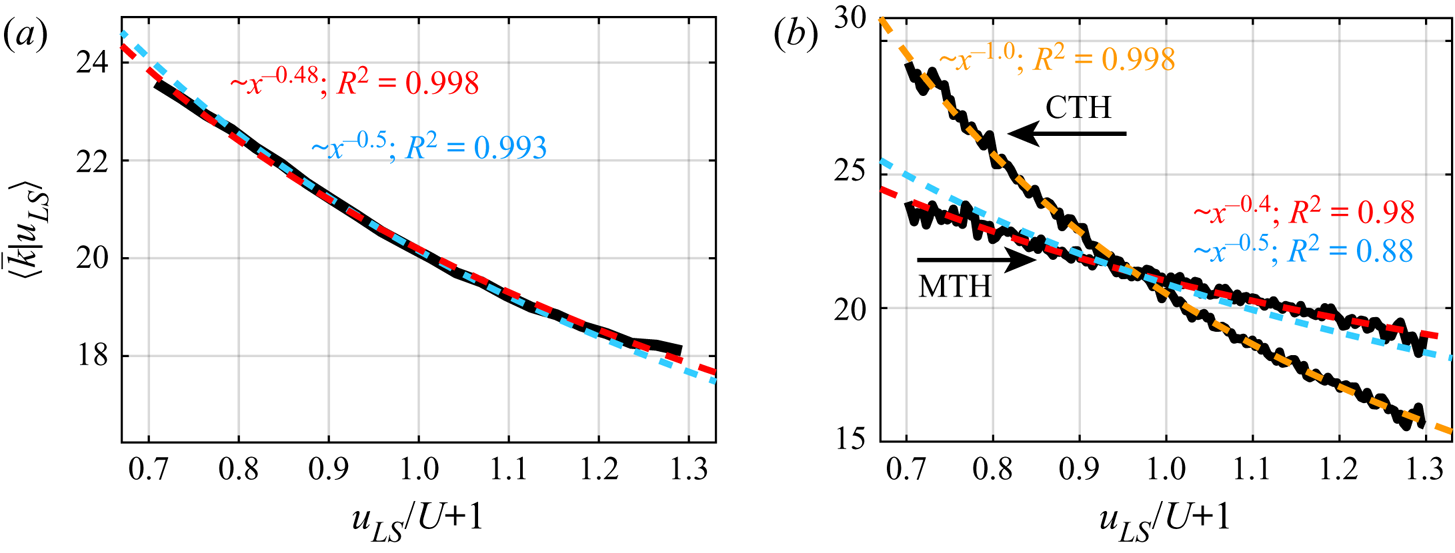
Figure 6. Average degree conditioned to the  $u_{LS}$ values as a function of the normalized
  $u_{LS}$ deviation, for
  $u$ signals at
  $y^+\approx 10$ in (a) the turbulent channel flow and (b) the turbulent boundary layer (angular brackets indicate the average over time and homogeneous directions). In (b), the scaling for the spatial series obtained through the CTH and MTH are shown as black lines. The power-law fitting curves are shown as dashed lines, together with the exponent of the fitting and the coefficient of determination,
  $R^2$, for both set-ups. Light-blue dashed lines correspond to the expected scaling trends for the spatial data. The intervals of
  $u_{LS}/U+1$ in abscissa cover, for each set-up, a range from the
  $5$th to the
  $95$th percentile of all
  $u_{LS}$ at the selected vertical coordinate
  $y^+\approx 10$.
The conditional averages were performed here by using uniformly-binned intervals of  $u_{LS}$, whereas Baars et al. (Reference Baars, Hutchins and Marusic2017), by adopting a variable-interval scheme for conditional averages, reported a scaling of approximatively
  $0.8$ (instead of
  $1$) for the frequency in turbulent boundary layers over a wide range of
  ${\textit {Re}}_\tau$. They indicated that the discrepancy in the expected exponent might be caused by an inaccurate assumption that the small scales are convected at a fixed inner-scaled velocity. However, here we show that the expected scaling for
  $f$ is still obtained by assuming
  $U_c\propto (U_\tau +u_{\tau ,LS})$, which suggests that the discrepancy in the fitting in Baars et al. (Reference Baars, Hutchins and Marusic2017) might be related to different methodological arguments.
The relevance of the scaling shown in figure 6 is twofold. First, it demonstrates that, similarly to the near-wall AM (Baars et al. Reference Baars, Hutchins and Marusic2017), the near-wall FM agrees with the quasi-steady quasi-homogeneous hypothesis. Second, the outcomes of figure 6 further validate the capability of the visibility-based approach, which relies on the degree centrality, to capture FM in wall-bounded turbulence, as well as the validity of the MTH (4.1) in converting a time series into a spatial series.
4.3. Analysis of the spanwise and wall-normal velocity components
The application of the NVG approach to the spatial series of wall-normal,  $v(x)$, and spanwise,
  $w(x)$, velocity from the DNS of the turbulent channel flows is here reported. Figure 7(a) shows the ratio
  $K_{np}$ for the
  $v$ (black and green curves) and
  $w$ (red and purple curves) components as a function of
  $y^+$ for the two channel flows at different
  ${\textit {Re}}_\tau$. Here,
  $K_{np}>1$ is found in the near-wall region, which indicates a positive frequency modulation of the large scales on the small scales of
  $v$ and
  $w$. This result is consistent with the AM investigations, which show a similar modulating effect of the large scales on the small scales of the three velocity components (Hutchins & Marusic Reference Hutchins and Marusic2007b; Talluru et al. Reference Talluru, Baidya, Hutchins and Marusic2014; Yao et al. Reference Yao, Huang and Xu2018; Wu et al. Reference Wu, Christensen and Pantano2019). In particular, the trends shown in figure 7(a) are similar to that reported in figure 5(a) for the
  $u$ signals, although lower
  $K_{np}$ values are obtained from
  $v$ and
  $w$. Moreover, as for
  $u$, the FM of the small scales of
  $v$ and
  $w$ is weaker at lower Reynolds number, because smaller
  $K_{np}$ values are observed in the near-wall region for
  ${\textit {Re}}_\tau =1000$.
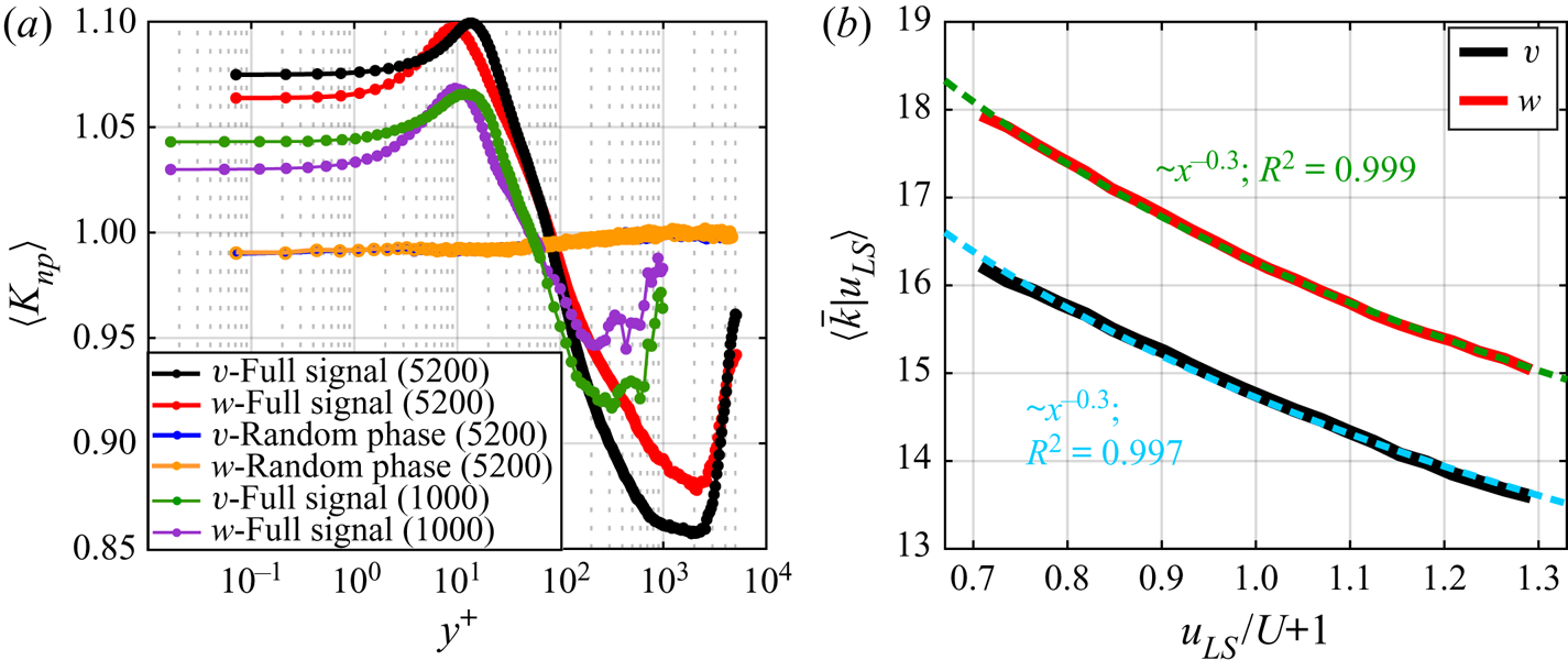
Figure 7. (a) The  $K_{np}$ ratio as a function
  $y^+$ for the wall-normal and spanwise velocity components,
  $v$ and
  $w$, extracted from the two channel-flow DNSs, together with the corresponding
  $K_{np}$ values for random-phase signals. The respective Reynolds number value of the DNS is reported within brackets in the legend. Angular brackets indicate averaging over time and the spanwise direction. (b) Average degree conditioned to the
  $u_{LS}$ values as a function of the normalized
  $u_{LS}$ deviation for
  $v$ and
  $w$ signals at
  $y^+\approx 10$ in the turbulent channel flow at
  ${\textit {Re}}_\tau \approx 5200$. The power-law fitting curves are shown as cyan and green dashed lines for the
  $v$ and
  $w$ cases, respectively, together with the exponents of the fitting and the coefficients of determination,
  $R^2$.
Furthermore, similar to the  $u$ component, an almost constant
  $K_{np}\approx 1$ behaviour is found for the network built from the random-phase
  $v$ and
  $w$ signals (see orange and blue curves in figure 7(a) referring to
  ${\textit {Re}}_\tau \approx 5200$ as a representative case), which confirms the ability of the degree to capture phase information from the (full) signal. It should be noted that, for the sake of consistency, a unique phase shuffling was performed in this case for the three velocity components. As the degree centrality from the
  $v$ and
  $w$ signals is conditionally averaged on
  $u_{LS}$, the phase of the streamwise velocity signal was extracted and randomly shuffled, so that the random-phase
  $u_{LS}$,
  $v$ and
  $w$ signals were obtained via the respective (non-shuffled) amplitudes but with the same random phases.
Although spectral peak separation in the spectrograms of the transversal velocity components is less evident than for the streamwise velocity, the generation and amplification of small-scale motions (i.e. fine-scale vortices) of all the three velocity components are strongly connected with large-scale events (Hutchins & Marusic Reference Hutchins and Marusic2007b). Within this perspective, the wall-normal and spanwise velocities are expected to be modulated in the near-wall region by following the QSQH hypothesis in a similar way as the streamwise component,  $u$. However, while results for AM of the three velocity components (Talluru et al. Reference Talluru, Baidya, Hutchins and Marusic2014; Agostini & Leschziner Reference Agostini and Leschziner2019; Chernyshenko Reference Chernyshenko2020) and scaling arguments for the AM and FM of the
  $u$ component (Baars et al. Reference Baars, Hutchins and Marusic2017) have been provided, as far as we know, similar scaling arguments (as in Baars et al. (Reference Baars, Hutchins and Marusic2017), figure 9 therein) for
  $v$ and
  $w$ have not been pursued for FM to date.
By analogy with the modulation of the  $u$ component, the conditional average degree,
  $(\bar {k}\,|\,u_{LS})$, is evaluated as a function of
  $(u_{LS}/U+1)$ at
  $y^+\approx 10$ for NVGs built from
  $v(x)$ and
  $w(x)$ signals. The conditional average degree and the corresponding fitting are shown in figure 7(b) for the
  ${\textit {Re}}_\tau \approx 5200$ set-up and confirm the power-law modulation effect of the large scales in the near-wall region even for the other velocity components, namely
  $k\propto (U+u_{LS})^{\beta _{v,x}}$ and
  $k\propto (U+u_{LS})^{\beta _{w,x}}$. However, while, for the
  $u$ component, the exponent of the power-law was
  $\beta _{u,x}\approx -0.5$, a weaker scale interaction effect was found for the
  $v$ and
  $w$ components, being
  $\beta _{v,x}\approx -0.3$ and
  $\beta _{w,x}\approx -0.3$, which are both smaller (in modulus) than
  $\beta _{u,x}$. This outcome is consistent with the smaller
  $K_{np}$ values for
  $v$ and
  $w$ (see figure 7a) than for
  $u$ (see figure 5a), which indicates a weaker FM in the near-wall region for the transversal velocity components.
The power-law relationships found for  $u$,
$u$,  $v$ and
  $w$ suggest that, although the intensity of modulation is different for each velocity component, the response of the small-scales of
  $v$ and
  $w$ exhibits a functional relation qualitatively analogous to the response of
  $u$. In general, there could be several factors playing a role in the scale-interaction mechanisms (such as the direction of the large scales as discussed by Chernyshenko Reference Chernyshenko2020), but we can conclude that the QSQH hypothesis is valid for all velocity components, although a more refined description is required for the transversal components,
  $v$ and
  $w$.
$w$.
The results shown in this section reveal that the three velocity components are all affected by a large-scale FM in the near-wall region, where an increase of the local (spatial) frequency is observed under  $u_{\tau ,LS}>0$ periods induced by positive
  $u_{LS}$ events. In particular, we provide novel insights on FM for the
  $v$ and
  $w$ components, which have been investigated less than
  $u$, in terms of FM intensity for the spatial series (figure 7a) and scaling arguments on the QSQH hypothesis (figure 7b).
4.4. Time and space shifting in FM
To conclude our analysis, we provide results on the investigation of the time- and space-shifted FM, as quantified by  $K_{np}$. We recall that a lead of the small-scale amplitude was found with respect to the large scales in the near-wall region of turbulent boundary layers, while a small-scale lag is found above the reversal coordinate (Bandyopadhyay & Hussain Reference Bandyopadhyay and Hussain1984; Guala et al. Reference Guala, Metzger and McKeon2011). Concerning FM, a lead of the small-scale frequency with respect to the large scales was found in the near-wall region but, different from AM, scattered behaviours were found far from the wall (Ganapathisubramani et al. Reference Ganapathisubramani, Hutchins, Monty, Chung and Marusic2012; Baars et al. Reference Baars, Talluru, Hutchins and Marusic2015).
To address this issue, in figure 8, we show the conditionally average degree,  $K_{np}$, as a function of
  $y^+$ and the spatial delay,
  ${\rm \Delta} r_x^+$, where for the time series, it holds the Taylor's hypothesis
  ${\rm \Delta} r_x^+=-U_c{\rm \Delta} t^+$ (the minus sign highlights the opposite direction of the reference systems between the fixed-point time series and spatial series). Therefore, the formulation of
  $K_{np}$ reported in (2.3a–c) is extended to account for spatial shifting,
  ${\rm \Delta} r_x^+$, as
  $K_{np}({\rm \Delta} r_x)=K_n({\rm \Delta} r_x)/K_p({\rm \Delta} r_x)$, with
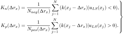 \begin{equation} \left.\begin{gathered} K_n({\rm \Delta} r_x)=\frac{1}{N_{neg}({\rm \Delta} r_x)} \sum_{j=1}^N {\left(k(x_j-{\rm \Delta} r_x)|u_{LS}(x_j)<0\right)},\\ K_p({\rm \Delta} r_x)=\frac{1}{N_{pos}({\rm \Delta} r_x)} \sum_{j=1}^N{\left(k(x_j-{\rm \Delta} r_x)|u_{LS}(x_j)>0\right)}. \end{gathered}\right\} \end{equation}
Positive or negative  ${\rm \Delta} r_x^+$ values indicate in (4.5) a lag or lead, respectively, of the degree,
  $k$, with respect to
  $u_{LS}$ in the conditional averages of (2.3a–c) (the results in figure 5 correspond to
  ${\rm \Delta} r_x^+={\rm \Delta} t^+=0$). If the CTH is employed for the turbulent boundary layer time series (figure 8a), a slight lead of
  $K_{np}$ with respect to
  $u_{LS}$ (i.e. high
  $K_{np}$ values are at
  ${\rm \Delta} r_x^+<0$ but close to
  ${\rm \Delta} r_x^+=0$) is observed for
  $y^+\lesssim 15$. However, a more substantial lead is observed for larger
  $y^+$ coordinates in the near-wall region up to
  $y^+\approx 100$, in agreement with previous analyses (Baars et al. Reference Baars, Talluru, Hutchins and Marusic2015), while a lag of
  $K_{np}$ with respect to large scales is detected for
  $y^+>rsim 100$. A clearer picture is obtained when the MTH is exploited (figure 8b). Significant lead of
  $K_{np}$ with respect to
  $u_{LS}$ is found in the whole near-wall region (including the wall proximity,
  $y^+\lesssim 15$), while the lag for
  $y^+>rsim 100$ is less evident and a lead is recovered for larger
  $y^+$ values (see blue contours in figure 8b). Eventually, no clear patterns are observed in the intermittent regions (
 $y^+>rsim 5\times 10^3$).
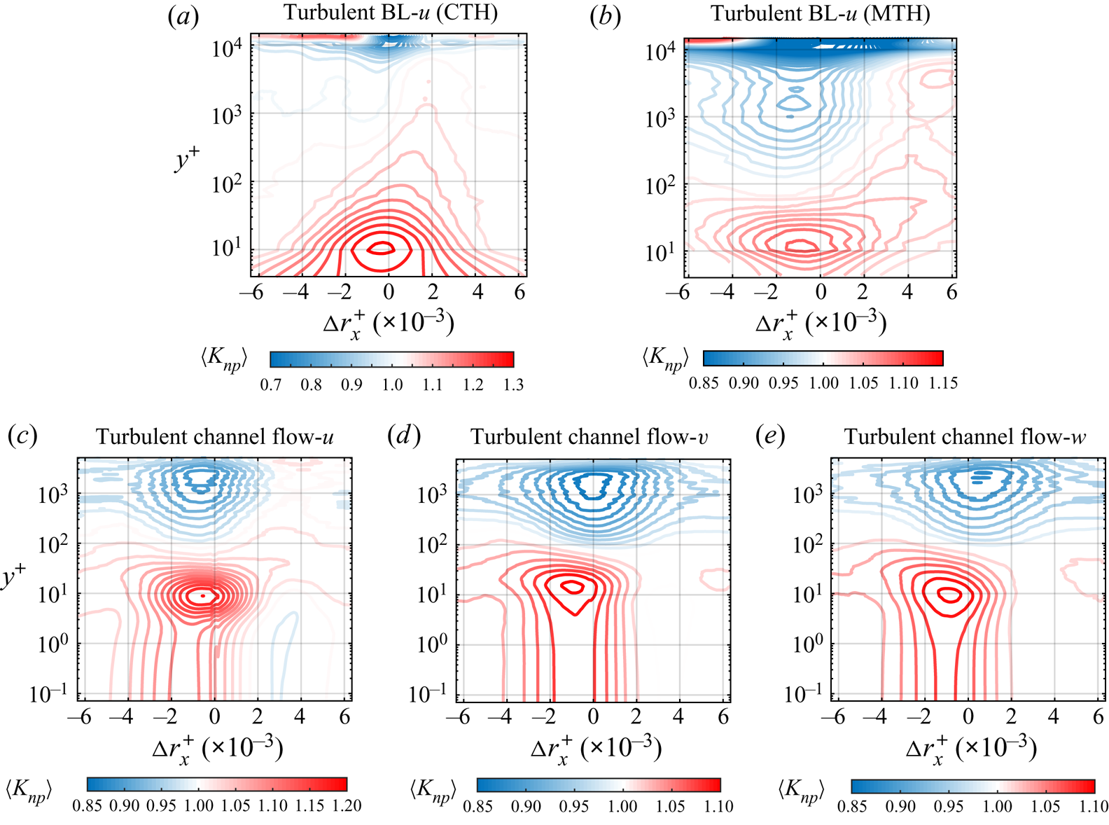
Figure 8. Contour plot of the  $K_{np}$ ratio as a function of the wall-normal coordinate,
  $y^+$, and the temporal or spatial shifting,
  ${\rm \Delta} t^+$ or
  ${\rm \Delta} r_x^+$, respectively. Shiftings for the turbulent boundary layer are reported in (a,b) whether the CTH or MTH is used, respectively. The spatial shifting for the turbulent channel flow at
  ${\textit {Re}}_\tau \approx 5200$ is shown in (c–e) for the three velocity components. Iso-level contours are displayed by using a level-step equal to
  $0.03$ in (a),
  $0.01$ in (b) and
  $0.015$ in (c–e).
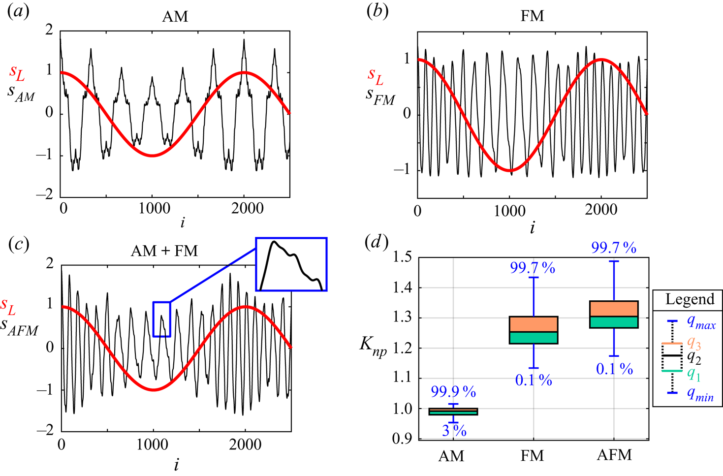
Figure 9. First 2500 time instants (out of  $10^4$) of the three synthetic modulated signals (shown in black) and the modulating signal (shown in red) for: (a) amplitude modulated signal (shown as AM); (b) frequency modulated signal (shown as FM); (c) amplitude and frequency modulated signal (shown as AM+FM). The inset shows a zoom of the AM+FM modulated signal. (d) Results of the application of the NVG to the synthetic signals in (a–c). Values of
  $K_{np}$ are shown as box plots, where
  $q_1$,
  $q_2$ and
  $q_3$ are the 25th, median, and 75th percentiles, respectively, while
  $q_{min}=q_1-1.5(q_3-q_1)$ and
  $q_{max}=q_1+1.5(q_3-q_1)$, whose values are explicitly indicated at the tips of the whiskers as percentages.
The space-shifted  $K_{np}$ values in the turbulent channel flow at
  ${\textit {Re}}_\tau \approx 5200$ for the three velocity components are displayed in figure 8(c–e). Similar to the turbulent boundary layer, a lead of
  $K_{np}$ with respect to
  $u_{LS}$ is found for
  $y^+<100$, as highlighted by high
  $K_{np}$ values for
  ${\rm \Delta} r_x^+<0$. Differences among the
  $u$,
$u$,  $v$ and
  $w$ components are detected in proximity of the channel centreline, where
  $K_{np}$ appears to lead, be in-phase and slightly lag
  $u_{LS}$ for the
  $u$ (figure 8c),
  $v$ (figure 8d), and
  $w$ components (figure 8e), respectively. It should be noted that the
  ${\textit {Re}}_\tau \approx 5200$ is here used as a representative set-up for spatial data, and the results for the lower
  ${\textit {Re}}_\tau$ channel flow are in agreement with the results in figure 8, so they are not shown for the sake of conciseness.
In particular, it is worth highlighting that the maximum  $K_{np}$ values in the near-wall region are found at
  ${\rm \Delta} r_x^+\approx 1000$ for the streamwise velocity in the turbulent boundary layer when the MTH is employed (figure 8b), as well as for all the velocity components in the turbulent channel flow (figure 8c–e). The value
  ${\rm \Delta} r_x^+\approx 1000$ is in excellent agreement with the characteristic length scale in the near-wall region, being
  $\lambda _x^+=O(10^3)$ (see inner spectral peak in figure 3a). The equivalent time scale is
  ${\rm \Delta} t^+={\rm \Delta} r_x^+/U_c^+\approx 100$ (being
  $U_c^+\approx 10$ in the buffer layer and viscous sublayer), which is the characteristic turnover time of the near-wall cycle. As the small scales are supposed to be actively modulated by the large scales, the time taken for this process to be completed is therefore equivalent to the time scale of the near-wall cycle (Ganapathisubramani et al. Reference Ganapathisubramani, Hutchins, Monty, Chung and Marusic2012).
The results shown in figure 8(a–c) for the streamwise velocity reveal that different convection velocities indeed play a significant role in the FM dynamics, not only in terms of overestimation (as highlighted in figure 5b), but also in terms of spatial delay that, in the near-wall region, is strongly related to the near-wall cycle. Therefore, NVG is again revealed to be a reliable approach for quantifying FM even in the presence of a temporal or spatial shifting. Finally, we note that an important issue about scale interaction is whether the large scales actually cause an increase or decrease of the small-scale activity, as the parameters used so far to quantify AM and FM only show that there is a relation (e.g. a correlation) between the large scales and small scales. Although definite answers to this issue are not still available, our detection of the presence of a significant temporal or spatial delay close to the characteristic time or length scale of the near-wall cycle, in conjunction with the arguments leading to relation (4.2), could provide supporting clues that a causation process is at play. In fact, fluctuations in the large-scale component of the wall shear stress, which affect the small-scale behaviour, appear to be directly caused by the outer large-scale structures rather than being the feature of near-wall processes (Zhang & Chernyshenko Reference Zhang and Chernyshenko2016).
5. Discussion
In this work, the natural visibility graph was used to study the 1-D spatial series and time series from two turbulent flow configurations, but some generalizations can be outlined. First, the geometrical criterion at the basis of the visibility algorithm can be extended to scalar fields of arbitrary dimension (Lacasa & Iacovacci Reference Lacasa and Iacovacci2017). For instance, Tokami et al. (Reference Tokami, Hachijo, Miyano and Gotoda2020) recently constructed a spatial visibility graph (employing a simplified version of the NVG, horizontal visibility graph, as proposed by Luque et al. Reference Luque, Lacasa, Ballesteros and Luque2009) from a 2-D velocity field in a buoyancy-driven turbulent fire. Therefore, our approach could be extended to 2-D velocity fields at fixed  $y^+$ coordinates, thus concurrently taking into account the degree variations along the streamwise and spanwise directions.
The results provided by natural visibility graphs, specifically about the degree centrality, necessarily depend on the signal resolution (either the sampling frequency or the grid size), which needs to be sufficiently high to capture the behaviour of the small scales. However, if the temporal or spatial resolution is sufficient to capture the smallest significant features of the signal, the degree centrality tends to proportionally scale with the signal resolution, as has already been shown, e.g. in Iacobello et al. (Reference Iacobello, Scarsoglio and Ridolfi2018b). Nevertheless, an additional feature of visibility networks is the possibility to explicitly account for the spatial or temporal discretization. In fact, one can assign to each discrete observation,  $i$, the corresponding signal spacing (e.g.
  ${\rm \Delta} x_i$,
  ${\rm \Delta} z_i$,
  ${\rm \Delta} t_i$, etc.). In this way, each node
  $i$ of the network is representative of an interval centred in
  $i$, thus providing a continuous representation of the signal. As a result, a weighted network is obtained in which the relation (2.2) is reformulated as
  $\tilde {k}_i\equiv \sum _j{{\rm \Delta} \chi _j A_{i,j}}$ for a series sampling,
  ${\rm \Delta} \chi _j$, where
  $\chi$ is independent variable (e.g. time). This generalization is particularly useful for non-uniformly sampled signals from experimental measurements, in which
  $\tilde {k}$ can be used in place of
  $k$, e.g. in the definition (2.3a–c).
Finally, it is worth observing that, so far, the visibility approach has been presented as a convexity criterion (see inequality (2.1)). In particular, the network degree was interpreted as a measure of the instantaneous period (quantified in terms of the local convexity of the signal), in analogy with the concept of instantaneous frequency based on the Hilbert transform (where the local properties of a series are emphasized by performing a convolution of the signal with the function  $1/t$ (Huang et al. Reference Huang, Shen, Long, Wu, Shih, Zheng, Yen, Tung and Liu1998)). Nevertheless, the visibility algorithm can also be used as a concavity criterion by applying it to the opposite signal,
  $-s_i$, whose effect is to change the direction in the inequality (2.1) (Iacobello et al. Reference Iacobello, Marro, Ridolfi, Salizzoni and Scarsoglio2019a). The comparison of the network metrics extracted from
  $s_i$ and
  $-s_i$ allows the characterization of the peak–pit asymmetry of a signal, especially in real-world phenomena (Hasson et al. Reference Hasson, Iacovacci, Davis, Flanagan, Tagliazucchi, Laufs and Lacasa2018). Following this point of view, we evaluated, for the sake of completeness, the values of
  $K_{np}(y^+)$ by using the NVG as a concavity criterion for the streamwise velocity, and we found that the main features of the FM for full and random-phase signals are retained when the information is only taken from either the convexity or concavity criterion.
6. Conclusions
In this study, we propose a novel approach to investigate the frequency modulation (FM) mechanism in wall-bounded turbulence by means of the natural visibility graphs. The spatial series and time series of the velocity from two turbulent channel flows and a turbulent boundary layer, respectively, are mapped into visibility networks and the degree centrality is conditionally averaged to the sign of the large-scale velocity to quantify FM. In particular, the versatility of visibility graphs to map either the time or spatial series, allows us to exploit the velocity spatial fields from turbulent channel flows that have been much less investigated than turbulent boundary layers under the lens of FM.
The overall results for the streamwise velocity indicate a FM mechanism occurring in the near-wall region with a peak of intensity in the buffer layer, in agreement with previous works. However, in contrast with the previous observations on FM, we observe a reversal in the FM mechanism far from the wall, similar to what is observed for AM, in both channel and boundary layer flows. We propose that such similarity could stem from a common underlying phenomenon, for which both the amplitude and frequency of the small scales are concurrently affected by negative or positive large-scale fluctuations. Moreover, we observe that the reversal coordinate scales as  ${{\textit {Re}}_\tau }^{0.5}$, which is reminiscent of the scaling in the wall-normal position of the outer spectral peak.
The effect of different convection velocities for the time series analysis is also discussed. In particular, we modify the correction proposed by Yang & Howland (Reference Yang and Howland2018) by accounting for only the large-scale velocity component in the definition of the convection velocity. This choice is based on the rationale that variations in the large-scale velocity induce variations in the wall shear stress, which, in turn, affect the behaviour of the small scales. We detect an overprediction of the FM when the local mean velocity is employed as the convection velocity in the turbulent boundary layer, while such overprediction is compensated when the proposed MTH is used. Moreover, scaling behaviours of the degree centrality as a function of the large-scale velocity are found to be in excellent agreement with the the QSQH theory. In this regard, our correction of the Taylor's hypothesis provides reliable scaling trends as the large-scale velocity is supposed to induce a modulation of the small scales through variations in the wall shear stress.
Finally, the FM for the wall-normal and spanwise velocity components is analysed for the turbulent channel flows and FM scaling is discussed for the transversal velocities. We find a FM mechanism for the wall-normal and spanwise velocity components qualitatively similar to FM of the streamwise velocity. Specifically, a power-law scaling of the degree conditioned to the large-scale velocity is found for the three velocity components, although smaller exponents are found for the transversal velocities than for the streamwise velocity. Moreover, a delay-based analysis is carried out for the three velocity components in the channel flow and for streamwise velocity time series in the boundary layer. We observe that the small scales lead the large scales in the near-wall region (in accordance with previous studies), but significant differences are found when the CTH or MTH is applied. Specifically, our MTH provides results in agreement with spatial series analysis, where the delay of maximum modulation corresponds to the characteristic length (or temporal) scale of the near-wall cycle.
Furthermore, we emphasize here that, to the best of our knowledge, this is the first time that FM is thoroughly investigated for all the three velocity components, as previous works have mainly focused on AM. The findings gained through the visibility networks of all the three velocities can then contribute to the development of a more general model of scale interaction, which accounts for the different modulating effect of the large scale on each velocity component.
The visibility-based approach reveals to be robust in the quantification of FM with respect to AM (Appendix A), and to different cut-off filtering sizes and high-frequency noise (Appendix B), as well as sensitive to a spectral phase randomization of the signals. The latter implies that the natural visibility graph is able to capture nonlinearities in the signal, as linear effects are preserved during phase randomization (i.e. amplitude spectrum does not change) while nonlinearities are lost through phase shuffling. We stress that the visibility networks do not require any a priori parameters and are directly built from the full velocity signals (instead of the small-scale component), because the network degree is able to capture the signal structure at the local scales. In this regard, although in this work a one-point analysis is carried out for simplicity, a two-point analysis (where the large-scale signal is extracted at a fixed wall-normal coordinate) would reveal the full potential of visibility networks. In fact, when multiple synchronized signals are available at different wall-normal locations (e.g. from numerical simulations, hot-wire rakes or through particle image velocimetry), the large-scale signal can be obtained only once at a fixed wall-normal location, and probes working on a smaller frequency range can be employed (as only low-frequencies are necessary). The full velocity signals, instead, can be used without any filtering operation to capture the small-scales frequency modulation at the remaining wall-normal locations.
In the wake of the recent successful applications of network science to the analysis of turbulent flows (Murugesan & Sujith Reference Murugesan and Sujith2015; Taira, Nair & Brunton Reference Taira, Nair and Brunton2016; Schlueter-Kuck & Dabiri Reference Schlueter-Kuck and Dabiri2017; Iacobello et al. Reference Iacobello, Scarsoglio, Kuerten and Ridolfi2019b; Krishnan et al. Reference Krishnan, Sujith, Marwan and Kurths2019), the proposed visibility-based approach is a candidate as a parameter-free and robust tool for FM investigation.
Declaration of interests
The authors report no conflict of interest.
Appendix A. Synthetic signals for visibility-based FM detection
In this appendix, we provide the results of the application of the visibility-based approach to quantify FM from synthetic signals, which is a simple but representative benchmark of more complex signals such as those from turbulent flow fields. Three configurations of modulation are here investigated, as shown in figure 9(a–c), namely amplitude modulation (AM), frequency modulation (FM) and both amplitude and frequency modulation (AM+FM). In this way, we assess the effect of different modulations on the ratio  $K_{np}$ and its ability to discern FM only.
All the generated signals have length  $N=10^4$ and sampling frequency
  $f_{samp}=4000$ Hz, which is chosen to be much larger than the characteristic frequencies of the modulated and modulating signals. The modulating (i.e. large-scale) signal, shown in red in figure 9(a–c), is given by the expression
  $s_L(t_i)=\cos (2{\rm \pi} f_L t_i)/3$, where
  $t_i=(i-1)/f_{samp}$ is the time, with
  $i=1,\ldots ,N$, and
  $f_L=2$ Hz is the frequency of the modulating signal.
The three modulated signals,  $s_{AM}$,
  $s_{FM}$ and
  $s_{AFM}$, are constructed as a high-frequency sinusoidal series, which emulate the small-scale velocity component, modulated by
  $s_L$. A positive modulation is considered, namely, an increase of amplitude and/or frequency is induced for intervals of positive
  $s_L$ values and vice versa for negative
  $s_L$ values. This behaviour mimics the modulation close to the wall by the large scales to the small scales in wall-bounded turbulence. Specifically, the three modulated signals, shown as black lines in figure 9(a–c), are given as
(i)
$s_{AM}=(\cos [2{\rm \pi} f_H t_i]+s_R)(1+s_L)$;(ii)
$s_{FM}=\cos [2{\rm \pi} f_H t_i + \varphi _L]+s_R$; and(iii)
$s_{AFM}=s_{FM}(1+s_L)$,


where  $f_H=12$ Hz is the (high) carrier-frequency of the modulated signals. The role of
  $(1+s_L)$ is to provide the AM effect on
  $s_{AM}$ and
  $s_{AFM}$, while the role of
  $\varphi _L$ is to give a frequency-modulated component to
  $s_{FM}$ and
  $s_{AFM}$. In particular,
  $\varphi _L$ is a time-varying phase depending on
  $s_L$ typically used to generate frequency-modulated signals (Boashash Reference Boashash2015), defined as
  $\varphi _L=2{\rm \pi} f_\varDelta I_m$, where
  $f_\varDelta =11$ Hz is the frequency deviation (i.e. the maximum frequency shift from
  $f_H$) and
  $I_m\equiv \sum _i{s_L(t_i)}/f_{samp}$. The frequency deviation,
  $f_\varDelta$, is selected to be close to the value of the carrier frequency,
  $f_H$, to maximize the modulation effect on the signal.
In each of the three modulated series, an additional signal,  $s_R$, is also included. It is obtained as a sum of unmodulated cosine signals with randomly-varying amplitude, given by
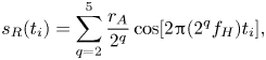 \begin{equation}
s_R(t_i)=\sum_{q=2}^5{\frac{r_A}{2^q}\cos[2{\rm \pi}(2^q
f_H)t_i]}, \end{equation}
\begin{equation}
s_R(t_i)=\sum_{q=2}^5{\frac{r_A}{2^q}\cos[2{\rm \pi}(2^q
f_H)t_i]}, \end{equation}
where  $r_A$ is a random number extracted from a uniform distribution in the range
  $(0,1)$. The effect of
  $s_R$ in a modulated signal can be observed in the inset of figure 9(c). The role of
  $s_R$ is to introduce – similar to turbulence velocity spectra – additional high-frequency low-amplitude components, thus making the modulated (small-scale) signal a broadband-like series.
By generating several random amplitudes,  $r_A$, in (A1), an ensemble of
  $s_R$ series is obtained for each
  $r_A$. This leads to an ensemble of different modulated signals,
  $s_{AM}$,
  $s_{FM}$ and
  $s_{AFM}$, which are characterized by different
  $s_R$. Specifically, we generated
  $5\times 10^3$ values of
  $r_A$ for each of the three modulated signals. The values of the ratio
  $K_{np}$ (see (2.3a–c)) are then computed for each ensemble, by evaluating the degree on the NVGs built for the full signals, namely,
  $(s_{AM}+s_L)$,
  $(s_{FM}+s_L)$ and
  $(s_{AFM}+s_L)$.
Figure 9(d) shows the values of  $K_{np}$ for the three modulation configurations as box plots, in which the most significant percentiles are highlighted. For the AM case,
  $K_{np}$ is concentrated around unity, with a median value that is very close to one, as is expected because the main modulating effect is on the amplitude. For the FM and AFM cases, instead, values of
  $K_{np}$ greater than one are consistently obtained (note the percentile values in figure 9d), as a result of the positive frequency modulating effect of the large-scale signal. In particular, it is worth noting that even when a signal is modulated both in amplitude and frequency, the ratio
  $K_{np}$ is able to emphasize the contribution of the FM.
The results shown in figure 9(d) reveal that  $K_{np}$ is an accurate parameter to quantify FM, because it consistently shows positive values under positive FM, and also a precise metric, because there is narrow spreading of the
  $K_{np}$ values around the median. The results shown in this appendix corroborate the ability and robustness of the proposed visibility-based approach, which relies on the conditioned degree centrality, to capture frequency modulation, thus fostering its application as a tool to study scale interaction in wall-bounded turbulence.
To conclude this section, we show the effect of higher frequency harmonics on the average degree,  $K$, for synthetic signals. With this aim, we use two sets of synthetic signals according to their power spectrum scaling following: (i) a
  $-5/3$ spectrum; and (ii) a
  $-2$ spectrum. The former emulates turbulent signals in the inertial range, while the second refers to signals defined in (A1). Figure 10(a,b) shows the power spectra for both types of synthetic signals, while figure 10(c) illustrates the behaviour of
  $K$ as a function of the maximum frequency considered,
  $f^*$. As discussed in § 2.2 referring to figure 3(c) for a turbulent series,
  $K$ decreases as the number of high-frequency harmonics increases. Moreover, the changes in
  $K$ are stronger for the synthetic signals following the
  $f^{-5/3}$ spectrum (figure 10a) than for the
  $f^{-2}$ spectrum (figure 10b), because the energy content of the small scales is larger in the former case, as the exponent
  $-5/3$ is lower (in modulus) than
  $-2$.
$-2$.
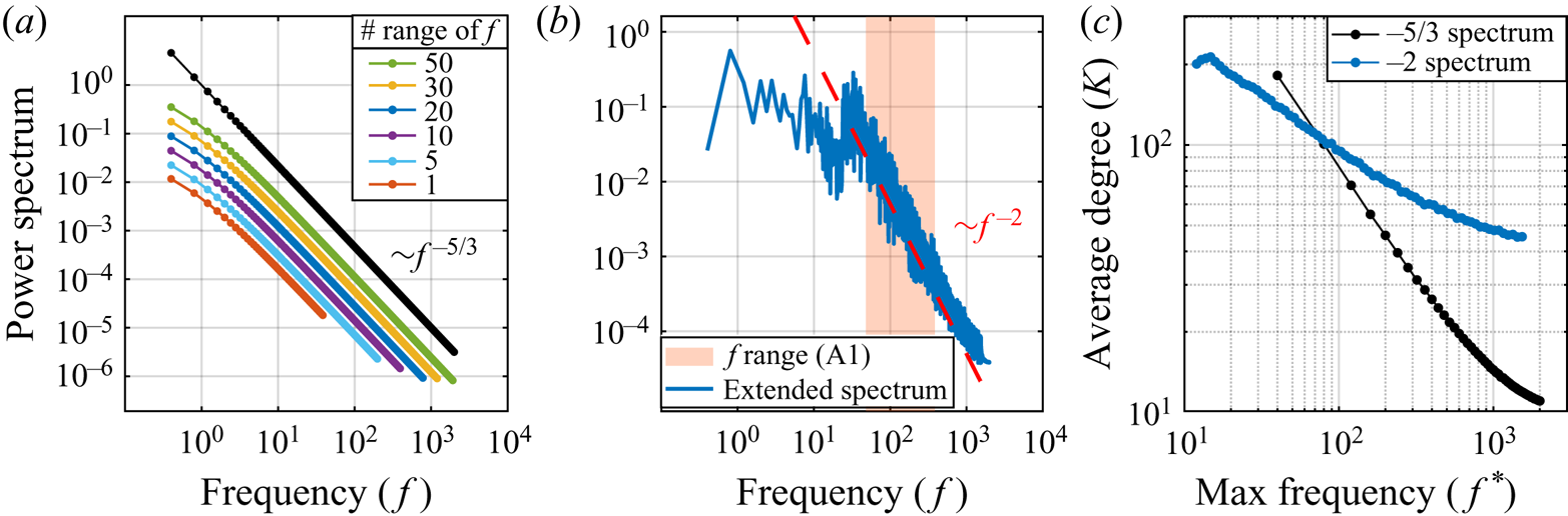
Figure 10. (a) Power spectra of synthetic signals following a  $f^{-5/3}$ law. Signals are generated through inverse-Fourier transform of the power spectrum shown in black for different frequency ranges (i.e. different number of harmonics). Fifty ranges of
  $f$ are generated, and the spectra of the synthetic signals for some representative
  $f$ ranges are highlighted with different colours, as well as vertically shifted to enhance visualization. (b) Power spectrum of signals generated as per (A1). The range of frequencies considered for the (A1) is highlighted as a shaded red region, and an
  $f^{-2}$ scaling is also shown. (c) Average degree centrality,
  $K$, for signals generated as in (a,b) for increasing maximum frequency,
  $f^*$.
Appendix B. Sensitivity analysis
The aim of this section is to assess the robustness of the proposed NVG-based approach under different values of the spectral filtering wavelength and under high-frequency noise.
We recall that the spectral filtering wavelength is used to extract the large-scale component,  $u_{LS}$, from the streamwise velocity signal,
  $u$. Mathis et al. (Reference Mathis, Hutchins and Marusic2009a) first reported a sensitivity analysis on the AM of streamwise velocity in a turbulent boundary layer. They showed that a decrease of the cut-off wavelength leads to a small increase of the AM below the reversal wall-normal coordinate (i.e. in the near-wall region) and a small decrease of AM above the reversal coordinate (i.e. far from the wall). The conclusion was that, despite the small variations arising from different cut-off wavelengths, the general form of the AM parameter is retained. For this reason, subsequent works on AM and FM exploited the sensitivity analysis by Mathis et al. (Reference Mathis, Hutchins and Marusic2009a) as a reference case to justify the choice of the cut-off wavelength.
Here we perform a sensitivity analysis on the wall-normal behaviour of  $K_{np}$ for the streamwise velocity by changing the cut-off wavelength,
  $\lambda _{x,c}$. Figure 11 shows
  $K_{np}$ as a function of
  $y^+$ for four
  $\lambda _{x,c}$ values, in the turbulent channel flow at
  ${\textit {Re}}_\tau \approx 5200$ (figure 11(a),
  $\lambda ^+_{x,c}=5186$ in the main text) and the turbulent boundary layer (figure 11(b),
  $\lambda ^+_{x,c}=7000$ in the main text). For the boundary layer, both the classical and modified Taylor's hypotheses are considered and labelled as CTH and MTH in the legend of figure 11(b). The nominal shape of
  $K_{np}$ as a function of
  $y^+$ is maintained for both the channel and boundary layers setups, and – similar to the analysis carried out by Mathis et al. (Reference Mathis, Hutchins and Marusic2009a) – a decrease in
  $\lambda _{x,c}$ leads to a reduction of
  $K_{np}$ below the reversal
  $y^+$ and a rise of
  $K_{np}$ above the reversal
  $y^+$. Specifically, variations of
  $K_{np}$ in the wall proximity are less evident for the boundary layer when the MTH is applied rather than when local mean velocity is considered as convection velocity (CTH).
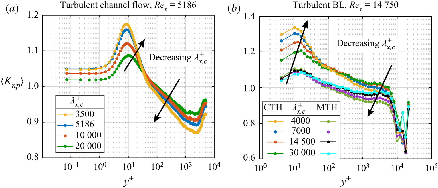
Figure 11. Effect of different cut-off wavelengths in the large-scale conditional average degree ratio,  $K_{np}(y^+)$, for streamwise velocity,
  $u$, extracted from (a) the channel flow DNS at
  ${\textit {Re}}_\tau \approx 5200$ and (b) the boundary layer experiments. In (b), the cut-off effect for spatial series obtained from the time series via the CTH, namely using as convection velocity the local mean velocity, and the MTH. Angular brackets indicate averaging over time and spanwise direction in (a) and over three different realizations in (b).
This sensitivity analysis confirms the robustness of the decoupling procedure to extract  $u_{LS}$, which is employed to evaluate
  $K_{np}$ as a metric for studying the FM.
Finally, our method is tested with the presence of high-frequency noise in the velocity signals (as usually happens in experimental measurements). With this aim, high-frequency noise is artificially added to the experimental signals of the streamwise velocity (whose sampling frequency is  $f_s=20\,000$ Hz) in the turbulent boundary layer. The noise signal is given by the sum of three harmonics with random phase and with frequencies equal to
  $0.5 f_s$,
  $0.475 f_s$ and
  $0.45 f_s$ (the maximum frequency included is
  $f_s/2$ as higher frequencies are not captured in the amplitude spectrum), whose effects on the spectra are displayed in figure 12(a). The corresponding values of
  $K_{np}$ are shown in figure 12(b), where we observe that the behaviour of
  $K_{np}$ is retained throughout the boundary layer except for the intermittency region, where the noise intensity significantly affects the signal structure. Therefore, we conclude that, although a pre-processing of the (experimental) data is always a good practice to avoid biased behaviours, the NVG approach based on
  $K_{np}$ is sufficiently robust under high-frequency noise.
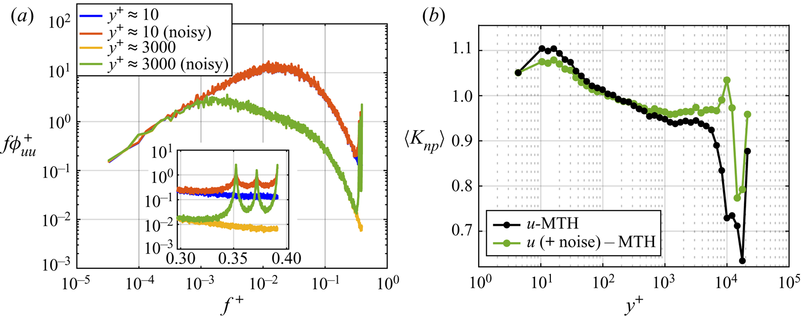
Figure 12. (a) Pre-multiplied energy spectrum of the streamwise velocity,  $uu$, from the turbulent boundary layer at two representative
  $y^+$ locations with and without high-frequency noise. The inset shows a zoom at the highest frequencies. (b) The
  $K_{np}$ as a function of
  $y^+$ for velocity signals without (black) and with (green) high-frequency noise (the MTH is used).


 $490 and
  $495), in which the small scales display enhanced or reduced activity, are also indicated.


