2.1. Wind tunnel facility

The Trisonic Wind Tunnel Munich (TWM) is a blow-down type wind tunnel with a $300\ \textrm {mm} \times 675\ \textrm {mm}$ ($w\times h$) test section. A two-throat system consisting of an adjustable Laval nozzle upstream of the test section and an adjustable diffuser downstream of the test section allows for a stable operating Mach number range from 0.3 to 3.0. The stagnation pressure is controlled by a pressure regulation valve and is adjustable between $p_0 = 1.2$ bar and $5.0$ bar. This allows the Reynolds number to be set independently of the Mach number. The corresponding Reynolds number ($Re_x$) range is $(4\text {--}78)\times 10^6\ \textrm {m}^{-1}$, which depends on the Mach number. The stagnation pressure $p_0$ and temperature $T_0$ are recorded by two sensors in the settling chamber. The facility has two storage tanks that can be pressurized up to 20 bar above ambient pressure, with each tank holding a volume of $178\ \textrm {m}^3$ of dry air. This amount of air is sufficient for run times in the order of 100 s for the cases discussed below. The wind tunnel's test section is enclosed by a plenum chamber and also has the ability to apply boundary layer suction at both the vertical and the horizontal walls independently. A detailed description of the freestream velocity and pressure fluctuations in the TWM can be found in Scharnowski, Bross & Kähler (Reference Scharnowski, Bross and Kähler2019).

A flat plate boundary layer model was mounted in the test section of the TWM for this investigation. A sketch of the model and coordinate system is shown in figure 1. The overall length of the model in the streamwise direction is 1.70 m, resulting in a turbulent boundary layer thickness of 13–27 mm at a location 1.26 m downstream of the leading edge. A cavity was milled out on the bottom side of the plate where a resistance based temperature sensor was installed in order to estimate the wall temperature $T_{w}$. The fluid properties in the freestream are calculated using the isentropic expansion equations and are denoted with the subscript $e$, e.g. the edge temperature $T_e$. Since the temperature of the wall is known and the static pressure at the edge is the same at the wall ($p_e=p_{w}$), $\rho _{w}$ can be calculated from the ideal gas law. The viscosity at the wall and the edge is estimated from the Sutherland Model, which is shown in (2.1) (Sutherland Reference Sutherland1883).

(2.1)\begin{equation} \frac{\mu_{w}}{\mu_{{ref}}}=\frac{T_{{ref}}+S}{T_{w}+S}\left(\frac{T_{w}}{T_{{ref}}}\right)^{3/2} \end{equation}

Figure 1. Flat plate boundary layer model used in the Trisonic Wind Tunnel Munich (TWM). Planar PIV measurement planes’ locations and orientations are indicated and labelled. The coordinates $(x,y,z)$ correspond to streamwise, spanwise and wall-normal directions respectively.

This model is applicable for dry air for a temperature range between 100 K and 1900 K where $S = 110.3\ \textrm {K}$ (Ames Research Staff 1953). A reference temperature $T_{{ref}} = 273\ \textrm {K}$ and viscosity $\mu _{{ref}} = 1.716 \times 10^{-5}\ (\textrm {kg}\,\textrm {ms}^{-1})$ was used. The fluid properties in the settling chamber and the test section are outlined in table 1 for the range of Mach numbers and Reynolds numbers considered in this investigation.

Table 1. Fluid properties at the edge ($e$) and surface of the flat plate or wall (w).

2.2. Turbulent boundary layer transition

Transitional devices affixed near the leading edge of aerodynamic surfaces are commonly used to ensure laminar/turbulent transition or to fix the transition location. These types of devices are often used to thicken the boundary layer, which is often desirable for measurements in high speed flows when the boundary layer thickness is very thin. However, these devices can produce unwanted flow features such as longitudinal vortices or a blockage that can influence coherent flow structures in turbulent incompressible boundary layers and condition the results of a measurement if an inadequate transition or perturbation is selected (Elsinga & Westerweel Reference Elsinga and Westerweel2012; Hutchins Reference Hutchins2012; Marusic et al. Reference Marusic, Chauhan, Kulandaivelu and Hutchins2015; Sanmiguel Vila et al. Reference Sanmiguel Vila, Vinuesa, Discetti, Ianiro, Schlatter and Örlü2017). Furthermore, it was shown (Bross, Scharnowski & Kähler Reference Bross, Scharnowski and Kähler2018) that even very conservative tripping devices with a height one half the laminar boundary layer thickness can produce a long wake that persists along the surface of the plate for a supersonic turbulent boundary layer, and it must be expected that they influence the near-wall flow features. Therefore, to avoid non-canonical flow perturbations, tripping devices were not applied to the leading edge of the flat plate boundary layer model used in this investigation.

To estimate the location of the natural (un-tripped) transition location for the subsonic and supersonic cases, oil film techniques were applied. A film of an oil mixture, consisting of petroleum oil, linseed oil, oleic acid and $\textrm {TiO}_2$ particles, was applied to the plate in a homogeneous manner by using a industrial paint sprayer device before each wind tunnel run. The aluminium plate surface was anodized black, which allowed for better contrast with the white $\textrm {TiO}_2$ particles. The oil film streaks then were captured with two side-by-side sCMOS cameras, creating a field of view spanning the entire test section width. The plate was illuminated with a white LED diffuse light source to create sufficient contrast and homogeneous illumination.

In addition, the flat plate model was designed with a sharp leading edge so that for the supersonic cases the strength of the shock is minimized by forcing an attached shock at the leading edge. For the subsonic case shown in figure 2(a) the sharp leading edge produces a small laminar separation which re-attaches approximately 6–7 mm downstream of the leading edge. An elliptically shaped leading edge can be used to avoid flow separation and reduce or eliminate unsteady loading on the plate or move the turbulence transition location downstream. However, for the investigation of a turbulent boundary layer developing over a long flat plate, the separation bubble at the leading edge for subsonic conditions can be considered as a type of transition element where the transition occurs in the shear layer at or near the bubble interface (Hain, Kähler & Radespiel Reference Hain, Kähler and Radespiel2009). Therefore, it can be expected that when the flow reattaches, a fully turbulent flow exists that includes a broad spectrum of turbulent scales and does not contain artificially generated coherent flow motions as typically found in the wake of transition devices. For the supersonic case shown in figure 2(b), the natural – i.e. unforced – transition location can be estimated by observing the transition wedge pattern near the leading edge. Transition wedges can only be observed where the flow is still laminar. Therefore, the transition location appears to be between 10 and 30 mm downstream of the leading edge for the subsonic and supersonic cases, respectively, which is very far upstream of the measurement location ($50\text {--}90\delta _{99}$ depending on the Mach number) so that enough boundary layer thickness turn-overs exist for the flow to develop.

Figure 2. Oil film visualization (a) $Ma = 0.3$ and $p_0 = 1.5$ and (b) $Ma = 2.0$ and $p_0 = 2.2$ in the leading edge region of the flat plate boundary layer model. The leading edge and spanwise boundaries of the plate are outlined with a white dashed line where $(x,y) = (0\ \textrm {mm},0\ \textrm {mm})$ is located at the leading edge and spanwise mid-point of the flat plate. Insert in (a) shows an enlarged more detailed view of the leading edge region for the subsonic case.

2.3. Side wall and corner effects

In order to characterize the effect of the side-wall boundary layer development and corner vortices, stereo-PIV (SPIV) measurements were performed in the cross-stream plane ($yz$-plane) approximately 1.3 m downstream of the leading edge of the flat plate shown in figure 1. The spanwise location of the measurement plane was adjusted such that both the side-wall of the wind tunnel and the flow extending approximately 100 mm towards the centre of the tunnel were visible. The results of this measurement for a supersonic and supersonic case are shown in figures 3(a) and 3(b).

Figure 3. Instantaneous streamwise velocity $u$ field normalized with $U_{\infty }$ in a spanwise ($y$) wall-normal ($z$) SPIV plane for (a) $Ma = 0.3$ and $p_0 = 1.5$ and (b) for $Ma = 2.0$ and $p_0 = 2.2$. (- -) contour lines correspond to lines of constant mean streamwise velocity $U$ for $U = 0.65$, 0.75, 0.95 and $0.99U_{\infty }$. In this plane, positive $u$ velocity is directed out of the page and $(y, z) = (0\ \textrm {mm}, 0\ \textrm {mm})$ correspond to the wind tunnel side wall and plate surface locations, respectively.

The presence of corner vortices and turbulent structures in the near side-wall and corner regions is evident from the instantaneous velocity fields for both subsonic and supersonic cases shown in figures 3(a) and 3(b). However, the influence of coherent flow motions seems to be limited to less than 60 mm from the side-wall. This is confirmed by the fact that contours of constant mean streamwise velocity corresponding to $U = 0.65$, 0.75 and $0.99U_{\infty }$ appear to converge for all wall-normal heights at spanwise distances greater than 60 mm. As the middle of the flat plate is located at 150 mm from the side wall, it can be concluded that the influences of the side-wall and corner flow are negligible in the centre of the test-section.

2.4. Quantitative flow field measurements via PIV

In order to quantitatively characterize the structural topology and spatial velocity statistical properties of the flow, velocity fields using PIV were obtained in three perpendicular planes as shown in figure 1. Planar 2-D-PIV was used in a streamwise wall-normal plane ($xz$-plane) and wall-parallel planes ($xy$-plane). In addition, SPIV measurements, different to the SPIV measurement setup shown in § 2.3 and centred at the midspan of the plate, were performed in the cross-stream direction ($yz$-plane); this provided all three velocity components ($u,v,w$).

The flow was seeded with Di-Ethyl-Hexyl-Sebacat (DEHS) tracer particles with a mean diameter of around $1 \ \mathrm {\mu }\textrm {m}$, as described by Kähler, Sammler & Kompenhans (Reference Kähler, Sammler and Kompenhans2002). The response time of these droplets is approximately $2\ \mathrm {\mu }\textrm {s}$ (Ragni et al. Reference Ragni, Schrijer, van Oudheusden and Scarano2011). A beam emanating from a Quantel Evergreen 200 Nd:YAG double pulsed laser was formed into a $500\ \mathrm {\mu }\textrm {m}$ thick light sheet in order to illuminate the tracer particles in the aforementioned measurement planes.

The PIV measurements analysed herein were obtained using classical double frame imaging, see Raffel et al. (Reference Raffel, Willert, Scarano, Kähler, Wereley and Kompenhans2018) for a detailed description of this measurement technique. Pairs of images are recorded separated by a short time delay $\Delta t$, and then sets of these double frame recordings are acquired in a sequence at a frequency of 15 Hz using specially suited sCMOS cameras. Approximately 1000 double frame recordings were acquired for each measurement case and nine different $\Delta t$ between $0.2\ \mathrm {\mu }\textrm {s}$ and $4\ \mathrm {\mu }\textrm {s}$ were used. The selection of the proper $\Delta t$ depended on both the optical magnification and the flow speed. In this case, the selected $\Delta t$ corresponded to a mean particle image shift between $\Delta x\approx 2$ pixels and 10 pixels close the wall and in the freestream, respectively. For all of the measurements, Makro-Planar Zeiss camera objectives were used to ensure excellent imaging quality. The PIV recordings were evaluated using state-of-the-art PIV software including multi-pass image deformation and Gaussian window weighting. The final interrogation window size was varied between $16\times 16$ pixels and $24\times 24$ pixels depending on the measurement plane, see table 2. The selection of the window size essentially fixes the spatial resolution of the measurement – i.e. the smallest possible length scale or structure that can be resolved corresponds to the size of the window as length scales smaller than the window size will be spatially low-pass filtered. However, since large-scale structures are the focus of this investigation, the spatial resolution of the presented measurements is sufficient; more details can be found in § 4. A $50\,\%$ window overlap was used, which made the final vector spacing half of the window size used for the particle image correlation.

Table 2. Imaging parameters for particle image velocimetry (PIV) measurements.

For each of the planes measured, a different camera and light sheet orientation was used. The streamwise wall-normal plane ($xz$-direction) was imaged by two sCMOS cameras which were mounted side by side in the $x$-direction such that they had overlapping fields of view (FOV) that observed the laser sheet perpendicularly. The recorded camera images were then stitched together resulting in a final field of view of $500\ \textrm {mm} \times 50\ \textrm {mm}$ (in $x$ and $z$, respectively) and scaling factor of $37.0\ \mathrm {\mu }\textrm {m}\,\textrm {pixels}^{-1}$. For this plane, the magnification, calculated by dividing the pixel pitch of the camera ($6.5\ \mathrm {\mu }\textrm {m}\,\textrm {px}^{-1}$) by the scaling factor, was $M = 0.18$. The wall-parallel plane ($xy$-direction) was imaged using one sCMOS camera that was mounted on top of the wind tunnel to view a wall-parallel aligned light sheet perpendicularly. In order to observe a relatively large FOV in the streamwise and spanwise directions, a short focal length camera objective was used, which resulted in a FOV of $180\ \textrm {mm}\times 140\ \textrm {mm}$ (in $x$ and $y$, respectively) with a scaling factor of $67.5\ \mathrm {\mu }\textrm {m}\,\textrm {pixels}^{-1}$ and magnification of $M = 0.10$. Finally, a higher resolution measurement was done in the cross-stream plane ($yz$-direction) where SPIV was used to measure all three perpendicular velocity components. The SPIV setup consisted of two sCMOS cameras mounted on the same side of the wind tunnel but aligned on either side of the cross-stream oriented light sheet. In this case the resulting FOV was $70\ \textrm {mm}\times 45\ \textrm {mm}$ (in $y$ and $z$, respectively) with a scaling factor of $26.1\ \mathrm {\mu }\textrm {m}\,\textrm {pixels}^{-1}$ and a magnification of $M = 0.42$. For the SPIV plane, all the Mach and Reynolds numbers listed in table 1 were measured, while for the wall-parallel plane, only $Ma = 0.3$ $p_0 = 1.5$, $Ma = 0.8$ $p_0 = 1.5$, $Ma = 2.0$ $p_0 = 2.2$ and $Ma = 3.0$ $p_0 = 4.5$, and were considered. Finally, for the streamwise wall-normal plane, only $Ma = 0.3$ $p_0 = 1.5$ and $Ma = 2.0$ $p_0 = 2.2$ were considered.

4.1. Streamwise-wall normal structures

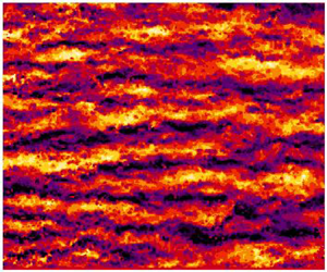
The organization of the turbulent boundary layer in the streamwise-wall-normal ($xz$) plane is considered first in this section as this is a commonly presented and discussed plane found in turbulent boundary layer literature. Figures 6(a) and 6(b) shows exemplary instantaneous velocity fields at $Ma = 0.3$, $p_0 = 1.5$ and $Ma = 2.0$, $p_0 = 2.2$ to illustrate typical structural features of the flow such as uniform momentum zones (UMZs). The streamwise extent of the measurement plane was produced by stitching two cameras aligned side by side with a small overlap in the streamwise field of view. The PIV images from each camera are evaluated separately and then the resulting velocity fields are stitched together in the overlap region.

Figure 6. Instantaneous velocity field $u/U_f$ in the $xz$-plane where $U_f = 0.99U_{\infty }$ at (a) $Ma = 0.3$, $p_0 = 1.5$ and (b) $Ma = 2.0$, $p_0 = 2.2$. Wall-normal, $z$, and streamwise, $x$, directions are scaled with $\delta _{99}$ which is 24.5 and 14 mm for $Ma = 0.3$, $p_0 = 1.5$ and $Ma = 2.0$, $p_0 = 2.2$ respectively. Solid black lines represent the turbulent–non-turbulent interface (TNTI) and solid grey contours lines of constant $u/U_f$ represent the borders or edges the uniform momentum zones (UMZs) determined from the relative probability function (p.d.f.) of the instantaneous velocity field $u/U_f$ for $Ma = 0.3$ and $Ma= 2.0$ in (c,d) respectively. The borders or edges of the UMZs, indicated with red-dashed lines, are located at the minima between the peaks present in the p.d.f. of $u/U_f$. Only the turbulent flow region, designated by the TNTI, was considered in the p.d.f. calculation.

A simple way of detecting features in the turbulent boundary layer is to look for regions of uniform momentum or so-called uniform momentum zones (UMZs). Detailed investigations about the presence of these regions or zones inside incompressible turbulent boundary layers can be found in Meinhart & Adrian (Reference Meinhart and Adrian1995) and Adrian et al. (Reference Adrian, Meinhart and Tomkins2000). More recently, de Silva, Hutchins & Marusic (Reference de Silva, Hutchins and Marusic2016) identified the presence of three to five UMZs using planar double-frame PIV measurements over a few orders of magnitude variation of high Reynolds numbers. These UMZs have also been described in the context of coherent structures as shown in Laskari et al. (Reference Laskari, de Kat, Hearst and Ganapathisubramani2018) where the temporal coherence of UMZs using time-resolved PIV of an incompressible ZPG turbulent boundary layer was explored. Within that study, the number of UMZs was related to the presence of a low- or high-momentum large-scale structure moving through the measurement plane. Therefore, the detection of UMZs can be used to interpret the instantaneous structure organization within a turbulent boundary layer.

As most of the previous studies have only considered incompressible flows, a brief demonstration of this detection technique applied to both the subsonic and supersonic measurements is provided. In figures 6(a) and 6(b) instantaneous colour contours of the velocity field $u/U_f$ in the $xz$-plane are plotted for the $Ma = 0.3$, $p_0 = 1.5$ and $Ma = 2.0$, $p_0 = 2.2$ cases. Overlaid on the colour contours are solid grey contour lines of constant $u/U_f$ that represent the edges or borders of the UMZs for these specific instantaneous velocity fields. In addition, the black solid line overlaid on these velocity fields represents the instantaneous turbulent–non-turbulent interface (TNTI), which was detected using the homogeneity criterion developed by Reuther & Kähler (Reference Reuther and Kähler2018).

The borders or edges of the UMZs are determined from the location of minima between the peaks in the relative probability function (p.d.f.) of $u/U_f$ shown in figures 6(c) and 6(d). The minima locations are indicated by the vertical red dashed lines and correspond to the values of constant $u/U_f$ used to draw the solid grey contour lines in figures 6(a) and 6(b). It should be noted that in order to avoid a large peak in the p.d.f. of $u/U_f$ near the boundary layer edge, an exclusion of any non-turbulent parts of the flow designated by the TNTI must be carried out before calculating the p.d.f. for each instantaneous flow field. Therefore, it follows that the TNTI forms the outermost edge or border of the UMZs in the turbulent boundary layer.

In the exemplary instantaneous fields shown in figures 6(a) and 6(b), four UMZs were detected for both the subsonic and supersonic cases. While an in-depth statistical analysis of the average number of UMZs was not performed, a survey of the instantaneous velocity fields showed a typical number of UMZs between two and four for both the sub- and supersonic cases, which is consistent with the number reported in the literature for incompressible turbulent boundary layers. In fact a recent study at hypersonic flow conditions detected two to three UMZs in the log-law layer and wake region at $Ma = 7.5$ (Williams et al. Reference Williams, Sahoo, Baumgartner and Smits2018). Therefore, it can be concluded that the organization of large-scale structures associated with UMZs in the outer flow region remains relatively unchanged for increasing Mach number.

It should be noted that the careful detection of the UMZ edges can depend on the spatial resolution (de Silva et al. Reference de Silva, Philip, Hutchins and Marusic2017) of the measurement, particularly in the wall normal direction. Due to the resolution limitations in all the aforementioned literature, including the results analysed herein, the region below $z/\delta < 0.1$ was not well resolved. However, it follows from the known coherent structures in the near-wall region, such as meandering streaks, and their dynamics that UMZs must also exist close to the wall. The presence of near-wall UMZs associated with the viscous sublayer and near-wall streaks was demonstrated in Bross et al. (Reference Bross, Fuchs and Kähler2019) in high spatial and temporal resolved near-wall particle tracking measurements of an incompressible turbulent boundary layer. Therefore, the detection of more UMZs in the compressible data discussed herein would be expected if the spatial resolution in the wall-normal direction was higher. However, as the focus of the present study is on the characteristics of large-scale structures in the outer flow region, the spatial resolution of the present measurements is sufficient.

To determine the mean streamwise elongation of the large-scale coherent flow motions from the correlation of streamwise velocity fluctuations, $u^{\prime }$, a two point spatial correlation analysis was performed. Plotted in figures 7(a) and 7(b) are contours of the correlation coefficient $R_{uu}$ at a wall-normal origin location $z_0/\delta _{99} = 0.2$, where $\xi _x = x_o + \Delta x$ with $x_0$ corresponding to the centre of the FOV in the streamwise direction. Overlaid on the colour contours is a straight line through the centre of the correlations with an inclination angle of $14^{\circ }$. For both the sub- and supersonic cases, the correlation at $z_0/\delta _{99} = 0.2$ appears to have a typical inclination angle of approximately $14^{\circ }$. This is consistent with the inclination angle of the large-scale motions which is widely reported for incompressible ZPG flows, between $12^{\circ }$ and $16^{\circ }$ (Adrian et al. Reference Adrian, Meinhart and Tomkins2000; Marusic & Heuer Reference Marusic and Heuer2007; Baars, Hutchins & Marusic Reference Baars, Hutchins and Marusic2017).

Figure 7. Two-point correlation coefficient $R_{uu}$, calculated at the wall-normal origin location $z_0/\delta _{99} = 0.2$ for (a) $Ma = 0.3$, $p_0 = 1.5$ and (b) $Ma = 2.0$, $p_0 = 2.2$. Horizontal axis is $\xi _x = x_0 + \Delta x$ where $x_0$ is the centre of the field of view. Solid black contour lines range from 0.2 to 1 in 0.1 increments. White dashed line is plotted with $14^{\circ }$ inclination angle.

Investigations in compressible flows vary in their results. Rayleigh scattering visualization of density fluctuations from Smith & Smits (Reference Smith and Smits1995) estimate between $30^{\circ }$ and $60^{\circ }$ inclination angle at $Ma = 2.5$. Similarly, multi-probe cross-correlation of hot-wire signals in a $Ma = 3.0$ turbulent boundary layer report inclinations angles of $(u \rho )^{\prime }$ based structures in the same range as Smith & Smits (Reference Smith and Smits1995). In contrast, correlations of $u^{\prime }$ from PIV measurements of at $Ma = 0.8$ turbulent boundary layers report inclination angles of $12^{\circ }$ and $13^{\circ }$ (Buchmann et al. Reference Buchmann, Cierpka, Knopp, Schanz, Schröder, Hain and Kähler2014) and DNS at $Ma = 3.0$ of $17^{\circ }$ and $20^{\circ }$ (Ringuette et al. Reference Ringuette, Wu and Martín2008). Pirozzoli & Bernardini (Reference Pirozzoli and Bernardini2011) also report a typical structure angle based on $u^{\prime }$ of around $14^{\circ }$ in their DNS at $Ma = 2.0$. However, Pirozzoli & Bernardini (Reference Pirozzoli and Bernardini2011) also report that the structure angles based on density and temperature fluctuations are typically two times larger than the $u^{\prime }$ structures. This explains why the inclination angles measured with Rayleigh scattering (Smith & Smits Reference Smith and Smits1995) and hot-wires (Spina, Donovan & Smits Reference Spina, Donovan and Smits1991) in compressible flows are much larger than the velocity based angle calculation.

Considering the streamwise extent of $R_{uu}$, the correlation appears to be slightly longer (${\sim }20\,\%$ increase) for the supersonic case in comparison to $Ma = 0.3$. However, due to low-level correlation below 0.2 with the surrounding field for $Ma = 0.3$, conclusions about the spatial extent of these low correlation values must be made with caution. This low-level correlation could be related to the fact that the nominal freestream turbulence intensity level in this particular blow-down wind tunnel is larger at $Ma = 0.3$ than at $Ma = 2.0$ (Scharnowski et al. Reference Scharnowski, Bross and Kähler2019). Nevertheless, the contour lines corresponding to $R_{uu} = 0.2$ undoubtedly appear slightly larger in the streamwise direction.

To examine the dominant frequencies associated with the coherent flow motions, the spectrogram of pre-multiplied power spectral density (PSD) was calculated for $Ma = 0.3$ and 2.0 and is plotted in figures 8(a) and 8(b). While the velocity fields measured with PIV in this case are only acquired at 15 Hz, the relatively large field of view allows for the spectral content in a spatial sense to be calculated without the assumption of Taylor's hypothesis of frozen turbulence. The $PSD$ was computed from vector fields based on an interrogation window size of $\textrm {IW} = 16 \times 16$ pixels with $50\,\%$ overlap using the method of Welch (Reference Welch1967). The $PSD$ was calculated at each wall normal position using a single Hamming window corresponding to FOV length in the streamwise distance for 1000 statistically independent velocity fields. The spectra for each time step were then averaged together to produce the final $PSD$ spectrograms.

Figure 8. Pre-multiplied streamwise velocity spectrogram $(\bar {\rho }/\rho _{w}) k_x \varPhi _{uu}/u_{\tau }^2$ for (a) $Ma = 0.3$, $p_0 = 1.5$ and (b) $Ma = 2.0$, $p_0 = 2.2$ as a function of streamwise wave length, $\lambda _x$ and wall-normal direction, $z$ scaled with $\delta _{99}$. Solid contour lines correspond to $(\bar {\rho }/\rho _{w}) k_x \varPhi _{uu}/u_{\tau }^2 = 1.1$, 1.2 and 1.3. The vertical and horizontal axis limits are the same in (a) as in (b).

The highest resolvable frequency is limited by the vector spacing of the velocity fields and effectively sets the spatial resolution of the measurement. Therefore, the wavelength of the largest resolvable frequency corresponds to the distance between two interrogation windows. With an IW of size $16\ \textrm {px} \times 16\ \textrm {px}$ the minimum resolvable wavelength corresponds to $\lambda = 0.6\ \textrm {mm}$. Likewise, the maximum resolvable wavelength corresponds to the FOV size. However, the $PSD$ is actually over sampled due to overlapping interrogation windows, which then corresponds to minimum resolvable wavelengths of 0.3 mm. However, it is important to note that the $PSD$ for spatial frequencies higher than (2/IW) does not satisfy the Nyquist criterion and are within the noise floor. Thus, the resolved wavelength range is from 0.6 mm to 175 mm in the streamwise direction, which is sufficient to resolve the features of the large-scale structures.

In these plots the largest values of normalized pre-multiplied velocity spectra, $(\bar {\rho }/\rho _{w}) k_x \varPhi _{uu}/u_{\tau }^2$, appear in a concentrated region with a maximum at a streamwise wavelength of $\lambda _x/\delta _{99}\approx 4.1$ and 5 for Mach 0.3 and 2.0, respectively, which corresponds to about a $20\,\%$ increase. While measurements closer to the wall were not possible in these experiments, this peak in the spatial spectral plots is indicative of the secondary peak (Fernholz & Finley Reference Fernholz and Finley1996; Monty et al. Reference Monty, Hutchins, NG, Marusic and Chong2009; Samie et al. Reference Samie, Marusic, Hutchins, Fu, Fan, Hultmark and Smits2018) in the streamwise velocity fluctuations. Since this peak is associated with the meandering superstructures in the log-law layer, it can be concluded that the superstructures are associated with slightly longer (by approximately ${\sim }20\,\%$) streamwise energetic wavelengths for $Ma = 2.0$ as compared to $Ma = 0.3$.

4.2. Cross-flow structures

In order to visualize and analyse the organization of coherent flow structures in the spanwise direction at different wall normal heights, SPIV measurements were performed in a cross-stream plane for all Mach numbers listed in table 1. Exemplary instantaneous velocity fields are shown in figures 9(a) and 9(b) to illustrate the slope and spanwise spacing of the large-scale structures. In the following, the characteristic spatial distribution of coherent structures in the spanwise direction via multi-point statistics and spatial spectral calculations are presented.

Figure 9. Instantaneous velocity field $u/U_f$ in the $yz$-plane or SPIV plane, where $U_f = 0.99U_{\infty }$ at (a) $Ma = 0.3$, $p_0 = 1.5$ and (b) $Ma = 2.0$, $p_0 = 2.2$. Wall-normal, $z$, and spanwise, $y$, directions are scaled with $\delta _{99}$, which is 24.5 and 14 mm for $Ma = 0.3$, $p_0 = 1.5$ and $Ma = 2.0$, $p_0 = 2.2$, respectively.

To quantify the average spacing of superstructures in the spanwise direction, two-point correlations of the streamwise velocity fluctuations in the spanwise direction for the range of Mach and Reynolds numbers was done. Shown in figures 10(a) and 10(b) are slices of the correlation coefficient $R_{uu}$ at $z_0/\delta _{99} = 0.2$ and 0.5. In these figures, the spanwise shift is represented as $\xi _y$, where $\xi _y = y_o + \Delta y$ with $y_0$ corresponding to the centre of the FOV in the spanwise direction.

Figure 10. Two-point correlation coefficient $R_{uu}$ slice across the spanwise direction at (a) $z_0/\delta _{99} = 0.2$ and (b) $z_0/\delta _{99} = 0.5$ for $0.3 \leq Ma \leq 3.0$. Plotted on the horizontal axis $\xi _y = y_0 + \Delta y$ where $y_0$ is the centre of the field of view in the spanwise direction and $\xi _y$ is scaled with $\delta _{99}$. Grey solid line represents incompressible reference $R_{uu}$ from DNS computations at $Re_{\tau } \approx 2000$ or $Re_{\theta } \approx 6500$ (Sillero, Jiménez & Moser Reference Sillero, Jiménez and Moser2013) of a ZPG turbulent boundary layer.

The slices of $R_{uu}$ at $z_0/\delta _{99} = 0.2$ interestingly reveal that there is a clear division between the correlations for $Ma < 1$ and the ones for $Ma > 1$. For $Ma < 1$ the distance between minimum correlation values is approximately $0.8\delta _{99}$, including the correlation result from a turbulent boundary layer incompressible DNS reference at $Re_{\tau } \approx 2000$ (Sillero et al. Reference Sillero, Jiménez and Moser2013). In contrast, for $Ma > 1$ the distance between minima is approximately $1.1\delta _{99}$, which is almost a $40\,\%$ increase from the subsonic cases. This implies that the spacing and or the width of superstructures increases rather discretely when the flow passes the sound barrier. Interestingly, this spacing increase appears to be independent of Mach number in the sense that no trend with Mach number is present except for the fact that the Mach number is either sub- or supersonic. Furthermore, the correlation is unaffected by Reynolds number since the correlations collapse for $Ma = 0.8$ $p_0 = 1.5$ and $p_0 = 3.0$ where $Re_{\delta _2}$ changes by a factor of two. The same collapse for the supersonic Reynolds number variation is also visible for $Ma = 2.0$ $p_0 = 2.2$ and $p_0 = 4.5$. A lack of the variation in the spanwise correlation length scales with Reynolds number was also confirmed in experimental investigations of incompressible turbulent boundary layers over several decades of Reynolds numbers in Hutchins & Marusic (Reference Hutchins and Marusic2007a). If a slice of the correlation is taken at $z_0/\delta _{99} = 0.5$ as shown in figure 10(b), the discrete increase in spacing from $Ma < 1$ to $Ma > 1$ is still visible although width of correlations has increased when compared to the spacing at $z_0/\delta _{99} = 0.2$. In addition, the width increase of $R_{uu}$ from subsonic to supersonic is only ${\sim }20\,\%$ at this wall location.

The apparent discrepancy between the subsonic and supersonic correlation results cannot be explained by the relative change in scaled spatial resolution due to the change in boundary layer thickness, as shown in figure 11. For all Mach numbers the same physical spatial resolution, which is fixed by the size of the IW, was used. With an $\textrm {IW} = 24 \times 24$ pixels the smallest resolvable spatial scale for $Ma = 0.8$ $p_0 = 1.5$ is $0.018\delta _{99}$ and $0.035\delta _{99}$ for $Ma = 2.0$ $p_0 = 2.2$. To show that this variation in relative spatial resolution does not influence the correlation results, $R_{uu}$ was calculated for different window size for $Ma = 0.8$ $p_0 = 1.5$ and $Ma = 2.0$ $p_0 = 2.2$ and is plotted in figure 11. For both the subsonic and supersonic cases a variation of IW size does not result in a change of the location of the correlation peaks, which indicates that the spatial resolution of the presented measurement is sufficient to resolve the spacing of the superstructures in the spanwise direction when scaled with $\delta _{99}$.

Figure 11. Two-point correlation coefficient $R_{uu}$ slice across the spanwise direction at $z_0/\delta _{99} = 0.2$ of $Ma = 0.8$, $p_0 = 1.5$ and $Ma = 2.0$, $p_0 = 2.2$ for different minimum spatial resolutions based on the PIV interrogation window (IW) size. Plotted on the horizontal axis $\xi _y = y_0 + \Delta y$ where $y_0$ is the centre of the field of view in the spanwise direction and $\xi _y$ is scaled with $\delta _{99}$.

To demonstrate that the apparent bi-modal behaviour of structure spacing for the sub- and supersonic cases shown in figures 10(a) and 10(b) is influenced by the scaling, the same slices of R$_{uu}$ are plotted in figures 12(a) and 12(b) except that $\xi _y$ is scaled with the displacement thickness $\delta ^*$. Since the displacement thickness calculation in (3.1) depends on the mean density variation across the layer, a Mach number dependent variation in the $\delta ^*$ scaled structure spacing, shown in figures 12(a) and 12(b), would be expected. Since $\delta ^*$ increases with Mach number, see table 3, the structure spacing also decreases when scaled with $\delta ^*$. The bi-modal behaviour is still visible in the sense that there is a large jump in the structure spacing when the sound barrier is crossed to $Ma = 2$, but the spacing then continues to decrease up to $Ma = 3$. In any case, both the $\delta _{99}$ and $\delta ^*$ scaling indicate that relative size or spacing of superstructures varies with Mach number. Since the majority of superstructure scales reported in the literature use $\delta _{99}$, the following analysis will also use $\delta _{99}$ for scaling.

Figure 12. Two-point correlation coefficient $R_{uu}$ slice across the spanwise direction at (a) $z_0/\delta _{99} = 0.2$ and (b) $z_0/\delta _{99} = 0.5$ for $0.3 \leq Ma \leq 3.0$. Plotted on the horizontal axis $\xi _y = y_0 + \Delta y$ where $y_0$ is the centre of the field of view in the spanwise direction and $\xi _y$ is scaled with the displacement thickness $\delta ^*$ (see (3.1)).

To confirm these findings at different wall normal distances, the spectra of the streamwise velocity pre-multiplied with the spanwise wave number as a function of spanwise wave lengths and wall normal distance for $Ma = 0.3$, $p_0 = 1.5$ and $Ma = 2.0$, $p_0 = 2.2$ are plotted in figures 13(a) and 13(b). The $PSD$ was computed from vector fields based on an interrogation window size of $\textrm {IW} = 24 \times 24$ pixels with $50\,\%$ overlap using in a similar way as in the previous section. The $PSD$ was calculated for each wall-normal position along the entire extent of the streamwise distance for 1000 statistically independent velocity fields. The resolvable spanwise ($\lambda _y$) wavelength range calculated in the PSD spectrogram is from 0.5 mm to 81 mm.

Figure 13. Pre-multiplied streamwise velocity spectrogram $(\bar {\rho }/\rho _{w}) k_y \varPhi _{uu}/u_{\tau }^2$ for (a) $Ma = 0.3$, $p_0 = 1.5$ and (b) $Ma = 2.0$, $p_0 = 2.2$ as a function of spanwise wavelength, $\lambda _y$, and wall-normal direction, $z$, scaled with $\delta _{99}$. The vertical and horizontal axis limits are the same in (a) as in (b).

The spectrograms plotted in figures 13(a) and 13(b) show both the wall-normal location and the spanwise wavelengths of spectral energy of streamwise velocity fluctuations in the cross-flow plane. The most energetic wavelengths for $Ma = 0.3$ vary between $\lambda _y = 0.7$ and $0.9\delta _{99}$, increasing slightly with wall-normal distance. Correspondingly, the most energetic wavelengths for $Ma = 2.0$ vary between $\lambda _y = 0.9$ and $1.2\delta _{99}$ with wall-normal distance. If these wavelengths are viewed as representative of the average spacing between two low- or high-momentum superstructures, the spectral results are consistent with the observations from the $R_{uu}$ slices in figures 10(a) and 10(b). Therefore, it can be concluded that compressibility has a clear influence on the spanwise spacing scaled with $\delta _{99}$ of superstructures identified based on velocity fluctuations.

4.3. Elongated structures in a wall parallel plane

To confirm directly that long high- and low-momentum meandering superstructures exist in the log-law region for the subsonic and supersonic cases investigated herein, PIV measurements in a wall-parallel plane ($xy$) were performed. Two exemplary instantaneous fields of the fluctuating streamwise velocity normalized with the local mean velocity ($u^{\prime }/\bar {u}$) are plotted in figures 14(a) and 14(b) for $Ma = 0.3$ $p_0 = 1.5$ and $Ma = 2.0$ $p_0 = 2.2$, respectively. The wall-parallel measurements were accomplished by aligning a laser light sheet parallel to the wall. Since the boundary layer thickness changes with Mach number, see table 3, the location of the measurement plane with respect to $z/\delta _{99}$ also changes with Mach number. Hence, the measurement plane was located at approximately $z/\delta _{99} = 0.1$ for the subsonic cases and at $z/\delta _{99} = 0.2$ for the supersonic cases. However, since both of these planes are located in the log-law layer, the presence of meandering superstructures in both the subsonic and supersonic cases is directly visible. Qualitatively, it can be seen that instantaneous high- and low-momentum structures can persist up to several boundary layer thicknesses and have a spanwise spacing of around one boundary layer thickness.

Figure 14. Instantaneous streamwise velocity fluctuation fields in the $xy$ plane for (a) $Ma = 0.3$, $p_0 = 1.5$ and (b) $Ma = 2.0$, $p_0 = 2.2$. The measurement plane is located at $z/\delta _{99} = 0.1$ and 0.2 for $Ma = 0.3$ and 2.0, respectively.

In the previous section, it was shown that the spatial correlations and spectral wavelengths associated with the spanwise spacing of the superstructures distinctly changes with Mach number. To confirm this finding in the wall-parallel plane, a spectral analysis of the streamwise velocity fluctuations in the spanwise direction was performed. Similar to the previous sections, a $PSD$ was calculated for each streamwise location along the entire spanwise distance of the FOV and then averaged together to produce the plot shown in figure 15(a). In this plot, the peak in the spectra is located just below $\lambda _y/\delta _{99} = 1$ for both subsonic cases and slightly above $\lambda _y/\delta _{99} = 1$ for the supersonic cases. While the location of the wall-parallel measurement plane was at slightly different $z/\delta _{99}$ locations for the subsonic and supersonic cases due to the changing boundary layer thickness, the finding that the structure spacing is larger for supersonic as compared to subsonic is consistent with the finding in the previous section, i.e. see figures 13(a) and 13(b).

Figure 15. (a) Pre-multiplied streamwise velocity spectra $(\bar {\rho }/\rho _{w}) k_y \varPhi _{uu}/u_{\tau }^2$ for $0.3 \leq Ma \leq 3.0$ vs. spanwise wavelength, $\lambda _y$ scaled with $\delta _{99}$. (b) Standard deviation $\sigma$ and mean $\mu$ of a normal distribution fit of the spanwise wavelengths $\lambda _y$ from (a) for each Mach number. Spectra calculated from wall-parallel planar PIV measurements.

For incompressible flows it has been shown that the amount or intensity of spanwise meandering of individual superstructures increases with wall-normal height (Kevin, Monty & Hutchins Reference Kevin, Monty and Hutchins2019). Since the measurements shown in figure 15(a) are located at slightly different $z/\delta _{99}$ locations, a quantitative analysis of the meandering magnitude might be influenced by wall-normal measurement location rather than the Mach number variation. However, for the wall-normal locations 0.1 and 0.2$\delta _{99}$ the meandering intensity variation is rather small (Kevin et al. Reference Kevin, Monty and Hutchins2019).

Instead of detecting individual structures and calculating their spanwise meandering frequency, the meandering influence on the spanwise length scale distribution for each Mach number can be deduced from a closer look at the spanwise spectra plotted in figure 15(a). The $PSD$ is calculated for all streamwise locations in the spanwise direction and ensemble averaged over all velocity fields. Therefore, the resulting average spectra plotted in figure 15(a) contains all the measurable frequencies/wavelengths of the $u^{\prime }$ fluctuations in the spanwise direction. Since a distinct energetic peak of $\lambda _y$ is visible for all Mach numbers, it can be concluded that there is only one structure ($\delta$ scaled) spacing or width present for each case. The distribution of the scales to the left and right of the maximum can then be related to the meandering nature of the superstructures. A more narrow distribution of spanwise wavelengths would mean that the structures meander less than if a wider distribution were present.

To look at this point more carefully, a normal distribution was fitted to the spanwise wavelengths, $\lambda _y$, in figure 15(a). The standard deviation ($\sigma$) and mean ($\mu$) of this fit for each Mach number in figure 15(a) are shown in figure 15(b). In addition to the peak $\lambda _y$ value ($\mu$) the width at 1$\sigma$ is also larger for the supersonic cases. This would then imply that the meandering of the superstructures is also influenced by Mach number. However, the distinct shift in the spanwise wavelength of the most energetic fluctuations or $\mu$ from the fit also indicates that the average superstructure spacing or width is larger for the supersonic cases when scaled with $\delta _{99}$.