


1. Introduction
Since friction drag in a turbulent flow is dominant in many industrial applications (Gad-el-Hak Reference Gad-el-Hak1994), turbulent friction drag reduction is of great importance for energy saving. To establish flow control methods for turbulent friction drag reduction in many practical situations, it is crucial to perform high-fidelity numerical simulations of controlled turbulent flows at reasonably high Reynolds numbers and find a scaling law applicable at practically high Reynolds numbers.
Flow control methods are classified into two categories: passive and active control methods. Although passive control methods, e.g. the use of riblets (Walsh Reference Walsh1983) and polymer additives (White & Mungal Reference White and Mungal2008) and bubble injection (Murai Reference Murai2014), have the advantage that their practical implementation is relatively easier, it is not always easy to put them into practice owing to the additional maintenance cost. On the other hand, although active control methods have the disadvantage that their implementation is more difficult owing to the requirement of a continuous energy input from an external system, their larger drag reduction effects encourage us to further investigate active control methods. In particular, predetermined control methods have a higher potential for drag reduction and the advantage of their easier implementation than feedback control methods, which have been widely investigated in terms of various approaches (Choi, Moin & Kim Reference Choi, Moin and Kim1994; Lee, Kim & Choi Reference Lee, Kim and Choi1998; Iwamoto, Suzuki & Kasagi Reference Iwamoto, Suzuki and Kasagi2002; Kim Reference Kim2003; Kim & Bewley Reference Kim and Bewley2007; Kasagi, Suzuki & Fukagata Reference Kasagi, Suzuki and Fukagata2009; Nakashima, Fukagata & Luhar Reference Nakashima, Fukagata and Luhar2017; Kawagoe et al. Reference Kawagoe, Nakashima, Luhar and Fukagata2019). Therefore, we can highly expect the practical use of predetermined control methods.
Among various predetermined control methods (e.g. Ricco, Skote & Leschziner Reference Ricco, Skote and Leschziner2021; Fukagata, Iwamoto & Hasegawa Reference Fukagata, Iwamoto and Hasegawa2024), streamwise travelling wave-like wall deformation is considered one of the most attractive control methods. Unlike streamwise travelling waves generated by blowing/suction (Min et al. Reference Min, Kang, Speyer and Kim2006; Lee, Min & Kim Reference Lee, Min and Kim2008; Lieu, Moarref & Jovanović Reference Lieu, Moarref and Jovanović2010; Moarref & Jovanović Reference Moarref and Jovanović2010; Mamori, Iwamoto & Murata Reference Mamori, Iwamoto and Murata2014; Koganezawa et al. Reference Koganezawa, Mitsuishi, Shimura, Iwamoto, Mamori and Murata2019; Ogino et al. Reference Ogino, Mamori, Fukushima, Fukudome and Yamamoto2019; Mamori et al. Reference Mamori, Fukudome, Ogino, Fukushima and Yamamoto2021), its implementation in industrial applications is expected to be relatively easier, as demonstrated by the experiment conducted by Suzuki et al. (Reference Suzuki, Shimura, Mitsuishi, Iwamoto and Murata2019), who used a rubber sheet driven by a single piezoelectric actuator. Nakanishi, Mamori & Fukagata (Reference Nakanishi, Mamori and Fukagata2012) investigated the control effect of a streamwise travelling wave generated by wall deformation in a low-Reynolds-number turbulent channel flow by direct numerical simulation (DNS). They achieved the relaminarization of the turbulent flow at a constant flow rate and bulk Reynolds number  $Re_b = 5600$, which corresponds to friction Reynolds number
  $Re_\tau \simeq 180$ in an uncontrolled flow. Nabae, Kawai & Fukagata (Reference Nabae, Kawai and Fukagata2020) revisited the same problem under a constant-pressure-gradient (CPG) condition at three different friction Reynolds numbers. Very recently, Albers, Shao & Schröder (Reference Albers, Shao and Schröder2024) have achieved a drag reduction of more than
  $50\,\%$ in a spatially developing compressible turbulent boundary layer flow using streamwise travelling wave-like wall deformation.
As a different control technique, a streamwise travelling wave of spanwise wall oscillation has been widely investigated (Ricco et al. Reference Ricco, Skote and Leschziner2021). Gatti & Quadrio (Reference Gatti and Quadrio2016) proposed a model for predicting the drag reduction rate at significantly high Reynolds numbers based on DNS results at low Reynolds numbers. Subsequently, for some specific parameter sets, the usefulness of this prediction model has been shown in recent studies (Marusic et al. Reference Marusic, Chandran, Rouhi, Fu, Wine, Holloway, Chung and Smits2021; Rouhi et al. Reference Rouhi, Fu, Chandran, Zampiron, Smits and Marusic2023) by conducting experiments up to  $Re_\tau = 12\,800$ and large-eddy simulation (LES) up to
  $Re_\tau = 4000$. In addition, Marusic et al. (Reference Marusic, Chandran, Rouhi, Fu, Wine, Holloway, Chung and Smits2021) proposed a new control strategy for drag reduction in a high-Reynolds-number turbulent flow. According to Marusic et al. (Reference Marusic, Chandran, Rouhi, Fu, Wine, Holloway, Chung and Smits2021), the contribution to the total wall shear stress from the large-eddy component increases as the Reynolds number increases: for example, the ratios of the large-eddy component to the total shear stress at
  $Re_\tau = 10^3$ and
  $10^5$ are about
  $8\,\%$ and
  $30\,\%$, respectively. By targeting this large-eddy component, they achieved substantial drag reduction at
  $Re_\tau = 12\,800$ by using a streamwise travelling wave with an oscillation period of more than
  $350$ in wall-unit time, which corresponds to ‘large-eddy actuation’ defined in their paper.
Unlike a travelling wave of spanwise wall oscillation, the drag reduction effect of a travelling wave generated by wall deformation has not been investigated even at moderately high Reynolds numbers  $Re_\tau \geqslant 10^3$ by either experiments or high-fidelity numerical simulations. To predict the drag reduction rate by streamwise travelling wave-like wall deformation over a wide range of friction Reynolds numbers, Nabae et al. (Reference Nabae, Kawai and Fukagata2020) proposed a semi-empirical formula for the mean velocity profile based on the scaling obtained by their DNS results. Their prediction implies that drag reduction rate of about 20 %–25 % was obtained even at practically high Reynolds numbers,
  $Re_\tau \sim 10^5\unicode{x2013}10^6$. In this semi-empirical formula, the Kármán constant was assumed to be unchanged by the control: similar to the prediction model proposed by Gatti & Quadrio (Reference Gatti and Quadrio2016), only a vertical shift of the mean velocity profile in the logarithmic region was considered. Note that Gatti & Quadrio (Reference Gatti and Quadrio2016) considered control using a streamwise travelling wave of spanwise wall oscillation. One cannot directly compare the drag reduction effect in the case of wall deformation with that in the case of wall oscillation because the pressure drag as well as the friction drag should be considered in the case of wall deformation. Therefore, to validate the semi-empirical formula proposed by Nabae et al. (Reference Nabae, Kawai and Fukagata2020) for practical large-scale turbulent flows, we should investigate the drag reduction effect in a high-Reynolds-number range where the logarithmic region in the mean velocity profile is clearly observed. According to a very classical estimation by Pope (Reference Pope2000), the logarithmic region is defined as
  $y^+ > 30$ and
  $y/\delta < 0.3$, where
  $y$ is the distance from the wall and
  $\delta$ is the channel half-width. Therefore,
  $Re_\tau > 10^3$ is required to obtain the logarithmic region of one decade.
As a useful high-fidelity numerical simulation technique, LES has been extensively utilized for the investigation of a turbulent flow at high Reynolds numbers. Since the pioneering study by Smagorinsky (Reference Smagorinsky1963), various subgrid-scale (SGS) models for LES have been proposed thus far (Meneveau & Katz Reference Meneveau and Katz2000; Moser, Haering & Yalla Reference Moser, Haering and Yalla2021). The Smagorinsky model (Smagorinsky Reference Smagorinsky1963) and wall-adapting local eddy-viscosity (WALE) model (Nicoud & Ducros Reference Nicoud and Ducros1999) are relatively simple eddy-viscosity models; thus, their implementation is easy and the required CPU time is small. However, the model constants used to determine model parameters, e.g. the Smagorinsky constant  $C_s$ (described in § 2), depend on flow fields: for example,
  $C_s = 0.2$ for homogeneous turbulence and
  $C_s = 0.1$ for turbulent channel flows. To solve this problem, the dynamic Smagorinsky model (DSM) (Germano et al. Reference Germano, Piomelli, Moin and Cabot1991; Lilly Reference Lilly1992) has been proposed. In the DSM, we can dynamically determine model parameters without any empirical model constants. However, the local determination of model parameters produces positive and negative model parameters, leading to numerical instabilities due to the negative viscosity. To remove the negative viscosity, the calculation of parameters in the DSM requires the averaging procedure in homogeneous directions of turbulent flows. Although this averaging procedure leads to numerical stability, more CPU time is required. In addition, under complex boundary conditions due to the flow control, e.g. wall deformation, the averaging procedure in the homogeneous directions is not reasonable. The validation of SGS models has been examined mainly in terms of uncontrolled canonical flows such as channel and boundary-layer flows. Although there are some LES studies on controlled flows (e.g. Chang, Collis & Ramakrishnan Reference Chang, Collis and Ramakrishnan2002), a detailed assessment of SGS models for controlled flows has not yet been realized.
On the basis of the above-mentioned background, the main objective of our present study is to investigate the drag reduction effect of streamwise travelling wave-like wall deformation in a turbulent channel flow at high Reynolds numbers of the order of  $Re_\tau \sim 10^3$ by using LES. First, we assess SGS models for the LES of a turbulent channel flow controlled using the streamwise travelling wave generated by wall deformation at low to moderate Reynolds numbers, i.e.
  $Re_\tau = 360$ and
  $720$. Subsequently, we investigate the drag reduction effect of streamwise travelling wave-like wall deformation at higher Reynolds numbers, i.e.
  $Re_\tau = 1080$,
  $2160$ and
  $3240$.
The rest of this paper is organized as follows. The numerical methods for the present LES and DNS are summarized in § 2. In § 3, we discuss the behaviour of several SGS models in a turbulent channel flow controlled using the streamwise travelling wave generated by wall deformation at  $Re_\tau = 360$ and
  $720$, and we compare it with the DNS results (Nabae et al. Reference Nabae, Kawai and Fukagata2020). In addition, we discuss the turbulent structures that are important for assessing the reproduction of the controlled flow. In § 4, we investigate the drag reduction effect of this control in high-Reynolds-number turbulent channel flows, i.e.
  $Re_\tau = 1080$,
  $2160$ and
  $3240$. Finally, we conclude the present study in § 5.
2. Numerical methods
2.1. Governing equation
The governing equations for LES are the filtered incompressible continuity and Navier–Stokes equations:
 $$\begin{gather} \frac{\partial u_i}{\partial x_i} = 0, \end{gather}$$
 $$\begin{gather}\frac{\partial u_i}{\partial t} ={-}\frac{\partial \left( u_i u_j \right)}{\partial x_j} - \frac{\partial p}{\partial x_i} + \frac{1}{\textit{Re}_\tau} \frac{\partial^2 u_i}{\partial x_j \partial x_j} - \frac{{\rm d} P}{{\rm d}\kern0.7pt x_1} \delta_{i1} - \frac{\partial \tau_{ij}}{\partial x_j}, \end{gather}$$
where  $u_i~( i=1,2,3 )$ and
  $p$ denote the filtered velocity components and pressure, respectively, and
  $\tau _{ij}$ is the SGS stress, which must be modelled to close the equations. The details of
  $\tau _{ij}$ are described later. All variables are made dimensionless by the fluid density
  $\rho ^*$, the friction velocity
  $u_\tau ^*$ and the channel half-width
  $\delta ^*$, where the superscript * denotes dimensional quantities. The friction Reynolds number is defined as
  $Re_\tau = u_\tau ^* \delta ^* / \nu ^*$, where
  $\nu ^*$ is the kinematic viscosity. The fourth term on the right-hand side of (2.2) representing the mean pressure gradient is
  $- ( {\rm d}P/{\rm d}\kern0.7pt x_1 ) = 1$. Hereafter, for convenience,
  $(x_1,x_2,x_3)$ and
  $(u_1,u_2,u_3)$ are interchangeably denoted by
  $(x,y,z)$ and
  $(u,v,w)$, respectively.
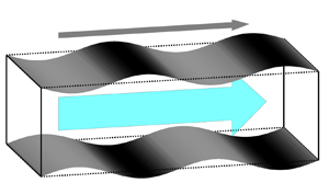
Figure 1 shows a schematic of a turbulent channel flow with streamwise travelling wave-like wall deformation. To compute the continuous deforming wall accurately, we utilize the coordinate transformation proposed by Kang & Choi (Reference Kang and Choi2000):
 \begin{equation} x = \xi_1,\quad y = \xi_2 \left( 1+\eta \right) + \eta_d,\quad z = \xi_3, \end{equation}
where  $\xi _1$,
  $\xi _2$ and
  $\xi _3$ are the streamwise, wall-normal and spanwise directions in computational space, respectively, and
  $\eta = ( \eta _u - \eta _d ) / 2$ with
  $\eta _u$ and
  $\eta _d$ denoting the displacements of the upper and lower walls, respectively. Similarly to previous studies (Nakanishi et al. Reference Nakanishi, Mamori and Fukagata2012; Nabae et al. Reference Nabae, Kawai and Fukagata2020; Nabae & Fukagata Reference Nabae and Fukagata2021), we apply the spanwise-uniform streamwise travelling wave; thus,
  $\eta _d$ and
  $\eta _u$ are defined as
 \begin{equation} \eta_d ={-}\frac{a}{kc} \sin \left \{ k \left( \xi_1 - ct \right) \right \},\quad \eta_u ={-}\eta_d. \end{equation}
For the surface motion, we consider the varicose mode, in which the upper and lower walls are moved in phase with the opposite sign. The control parameters used to determine the surface motion are the velocity amplitude  $a$, the streamwise wavenumber
  $k$ and the phase speed
  $c$. In this study, the combination of these control parameters is set to
  $( a^+,k^+,c^+ ) = ( 10,0.022,30 )$, which is the maximum drag reduction case in the paper by Nabae et al. (Reference Nabae, Kawai and Fukagata2020). Hereafter, a superscript ‘
 $+$’ denotes wall units.

Figure 1. Schematic of a turbulent channel flow with streamwise travelling wave-like wall deformation.
As a result of this coordinate transformation, the filtered continuity and Navier–Stokes equations in the boundary-fitted coordinates of (2.3a–c) are respectively expressed as
 $$\begin{gather} \frac{\partial u_i}{\partial \xi_i} ={-}S_c, \end{gather}$$
 $$\begin{gather}\frac{\partial u_i}{\partial t} ={-}\frac{\partial \left( u_i u_j \right)}{\partial \xi_j} - \frac{\partial p}{\partial \xi_i} + \frac{1}{\textit{Re}_\tau} \frac{\partial^2 u_i}{\partial \xi_j \partial \xi_j} - \frac{{\rm d}P}{{\rm d}\xi_1} \delta_{i1} +S_i - T_i, \end{gather}$$
where  $S_c$ and
  $S_i$ are the source terms due to the coordinate transformation:
 \begin{align} S_c &= \varphi^\prime_j \frac{\partial u_j}{\partial \xi_2}, \end{align}
 \begin{align} S_i &={-}\psi_t \frac{\partial u_i}{\partial \xi_2} - \varphi^\prime_j \frac{\partial \left( u_i u_j \right)}{\partial \xi_2} - \varphi^\prime_i \frac{\partial p}{\partial \xi_2} \nonumber\\ &\quad +\frac{1}{ \textit{Re}_\tau } \left \{ 2\varphi^\prime_j \frac{\partial^2 u_i}{\partial \xi_j \partial \xi_2} + \varphi^\prime_j \varphi^\prime_j \frac{\partial^2 u_i}{\partial \xi_2 \partial \xi_2} + \frac{1}{2} \frac{\partial \left( \varphi^\prime_j \varphi^\prime_j \right)}{\partial \xi_2} \frac{\partial u_i}{\partial \xi_2} + \frac{\partial \varphi^\prime_j}{\partial \xi_j} \frac{\partial u_i}{\partial \xi_2} \right \}, \end{align}
with
 $$\begin{gather} \psi_t ={-}\frac{1}{1+\eta} \left( \frac{\partial \eta_d}{\partial t} + \xi_2 \frac{\partial \eta}{\partial t} \right), \end{gather}$$
 $$\begin{gather}\varphi^\prime_j = \varphi_j - \delta_{j2} \end{gather}$$
and
 \begin{equation} \varphi_j = \left \{\begin{array}{@{}ll@{}} \displaystyle{ -\dfrac{1}{1+\eta} \left( \dfrac{\partial \eta_d}{\partial \xi_j} + \xi_2 \dfrac{\partial \eta}{\partial \xi_j} \right) } & {\rm for}\ j=1,3, \\ \displaystyle{ \dfrac{1}{1+\eta} } & {\rm for}\ j=2. \end{array}\right. \end{equation}
In addition, the SGS terms are transformed as follows:
 \begin{align} T_i &= \frac{\partial \tau_{ij}}{\partial x_j} \nonumber\\ &= \frac{\partial \tau_{ij}}{\partial \xi_k} \frac{\partial \xi_k}{\partial x_j} \nonumber\\ &= \left \{\begin{array}{@{}ll@{}} \displaystyle{ \dfrac{\partial \tau_{ij}}{\partial \xi_j} - \dfrac{\partial \tau_{ij}}{\partial \xi_2} \dfrac{1}{1+\eta} \left( \dfrac{\partial \eta_d}{\partial \xi_j} + \xi_2 \dfrac{\partial \eta}{\partial \xi_j} \right) } & {\rm for}\ j=1,3, \\ \displaystyle{ \dfrac{\partial \tau_{ij}}{\partial \xi_j} \dfrac{1}{1+\eta} } & {\rm for}\ j=2. \end{array} \right. \end{align}
 The periodic boundary conditions are applied in the streamwise  $( \xi _1 )$ and spanwise
  $( \xi _3 )$ directions. When considering the coordinate transformation associated with the wall deformation, the no-slip velocity boundary conditions on the upper and lower walls lead to
 \begin{equation} \left \{\begin{array}{@{}ll@{}} u_1 = u_3 = 0,~u_2 = \displaystyle{ \dfrac{\partial \eta_u}{\partial t} } ={-}a \cos \left \{ k \left( \xi_1 - ct \right) \right \} & {\rm (upper~wall),} \\[10pt] u_1 = u_3 = 0,~u_2 = \displaystyle{ \dfrac{\partial \eta_d}{\partial t} } = a \cos \left \{ k \left( \xi_1 - ct \right) \right \} & {\rm (lower~wall).} \end{array} \right. \end{equation}
2.2. Subgrid-scale models
In the present LES,  $\tau _{ij}$ is modelled on the basis of the eddy-viscosity assumption as
 \begin{equation} \tau_{ij} = \tfrac{1}{3} \tau_{kk} \delta_{ij} - 2 \nu_t s_{ij}, \end{equation}
where  $\nu _t$ denotes the SGS eddy viscosity and
  $s_{ij}$ is the strain-rate tensor, i.e.
  $s_{ij} = ( \partial u_j / \partial x_i + \partial u_i / \partial x_j ) / 2$. The SGS eddy viscosity
  $\nu _t$ should be modelled in LES. However, in an incompressible flow,
  $\tau _{kk}$ does not need to be modelled because it is solved with pressure as
  $p + \tau _{kk} / 3$. The SGS models used in this study are summarized below.
2.2.1. Smagorinsky model
The Smagorinsky model (Smagorinsky Reference Smagorinsky1963) is the most classical SGS model expressed as
 \begin{equation} \nu_t = f_v \left( C_s \bar{\varDelta} \right)^2 \sqrt{2 S^2}, \end{equation}
where  $S^2 = s_{ij} s_{ij}$ and the Smagorinsky constant
  $C_s$ is set to
  $0.1$ for turbulent channel flows (Pope Reference Pope2000). The filter width
  $\bar {\varDelta }$ is given by the geometric mean, i.e.
  $\bar {\varDelta } = ( \Delta \xi _1 \Delta \xi _2 \Delta \xi _3 )^{1/3}$, where
  $\Delta \xi _i$ is the grid spacing in the
  $i$th direction. The near-wall damping function
  $f_v$ is introduced to decrease the excessive SGS stress in the region near the wall. In this study, we consider the damping function used by Hwang & Cossu (Reference Hwang and Cossu2010):
 \begin{equation} f_v = 1-\exp \left[ - \left( \frac{y_d^+}{A^+} \right)^3 \right], \end{equation}
where  $y_d$ is the distance from the wall in computational space and
  $A^+ = 25$. In general, the classical van Driest damping function, i.e.
  $f_v = [ 1-\exp ( -y_d^+ / A^+ ) ]^2$, has been widely used as a damping function. However, according to our preliminary test in a sufficiently high-grid-resolution case (HR case, explained later), the Smagorinsky model using (2.16) predicts the drag reduction rate in DNS better than that predicted using the classical van Driest damping function (see Appendix A for details). Therefore, in this study, we utilize (2.16) as a damping function.
2.2.2. The WALE model
The WALE model (Nicoud & Ducros Reference Nicoud and Ducros1999) is based on the square of the velocity gradient tensor, and the SGS eddy viscosity is modelled as
 \begin{equation} \nu_t = f_v \left( C_w \bar{\varDelta} \right)^2 \frac{ \left( s_{ij}^d s_{ij}^d \right)^{3/2} }{ \left( s_{ij} s_{ij} \right)^{5/2} + \left( s_{ij}^d s_{ij}^d \right)^{5/4} }. \end{equation}
The square of the traceless symmetric part of the velocity gradient tensor,  $s_{ij}^d s_{ij}^d$, is computed as
 \begin{equation} s_{ij}^d s_{ij}^d = \tfrac{1}{6} \left( S^2 S^2 + \varOmega^2 \varOmega^2 \right) + \tfrac{2}{3} S^2 \varOmega^2 + 2 IV_{S \varOmega}, \end{equation}
with  $\varOmega ^2 = \omega _{ij} \omega _{ij}$ and
  $IV_{S \varOmega } = s_{ik} s_{kj} \omega _{jl} \omega _{li}$, where
  $\omega _{ij}$ is the rotation tensor, i.e.
  $\omega _{ij} = ( \partial u_j / \partial x_i - \partial u_i / \partial x_j ) / 2$. The constant
  $C_w$ is set to
  $0.5$. Here, we introduce an additional damping function
  $f_v$ of (2.16) to the WALE model because the original WALE model where
  $f_v = 1$ does not reproduce the decrease in eddy viscosity in the near-wall region when considering the travelling wave generated by wall deformation (see Appendices A and B).
2.3. Numerical schemes and conditions
The LES code in this study is based on the DNS code for an uncontrolled turbulent channel flow developed in previous studies (Fukagata, Kasagi & Koumoutsakos Reference Fukagata, Kasagi and Koumoutsakos2006; Nabae & Fukagata Reference Nabae and Fukagata2024) and that used by Nabae et al. (Reference Nabae, Kawai and Fukagata2020), who performed the DNS of a turbulent channel flow controlled using the spanwise-uniform travelling wave generated by wall deformation under the CPG condition. The governing equations are spatially discretized using the energy-conserving fourth-order finite-difference scheme (Morinishi et al. Reference Morinishi, Lund, Vasilyev and Moin1998) in the streamwise and spanwise directions and the second-order finite-difference scheme in the wall-normal direction on the staggered grid system. For time integration, we utilize the low-storage, third-order Runge–Kutta/Crank–Nicolson scheme (Spalart, Moser & Rogers Reference Spalart, Moser and Rogers1991) with the high-order SMAC-like velocity–pressure coupling scheme (Dukowicz & Dvinsky Reference Dukowicz and Dvinsky1992). The pressure Poisson equation is solved by a two-dimensional fast Fourier transform in the streamwise and spanwise directions and using the tridiagonal matrix algorithm in the wall-normal direction.
Similarly to Nabae et al. (Reference Nabae, Kawai and Fukagata2020), all simulations in this study are performed under CPG conditions because the near-wall scaling is of great importance for predicting the drag reduction rate by the modelling of the mean velocity profile. We consider five different friction Reynolds numbers, i.e.  $Re_\tau = 360$,
  $720$,
  $1080$,
  $2160$ and
  $3240$. The computational conditions are shown in table 1, where
  $L_i$ and
  $N_i$ denote the length of the computational domain and the number of grid points, respectively, in the
  $i$th direction. In table 1, ‘no model’ represents the simulations without using any SGS models.
Table 1. Computational conditions in all cases.

All simulations at  $Re_\tau = 360$ are classified into four different categories on the basis of grid resolution and domain size: the ZHR, XHR, HR and HR-SD cases. Cases ZHR and XHR represent higher grid resolutions in the
  $z$ and
  $x$ directions, respectively: in the ZHR case,
  $( \Delta x^+,\Delta z^+ ) = ( 35.3,17.7 )$; in the XHR case,
  $( \Delta x^+,\Delta z^+ ) = ( 23.6,23.6 )$. Case HR represents higher grid resolution in both the
  $x$ and
  $z$ directions, i.e.
  $( \Delta x^+,\Delta z^+ ) = ( 23.6,17.7 )$. The numbers of grid points in the streamwise direction per wave,
  $N_w$, are
  $N_w = 8$,
  $12$ and
  $12$ in the ZHR, XHR and HR cases, respectively, whereas
  $N_w = 32$ in DNS (Nabae et al. Reference Nabae, Kawai and Fukagata2020). In addition, the computational domain in the ZHR, XHR and HR cases is
  $( L_x,L_y,L_z ) = ( 2{\rm \pi},2,{\rm \pi} )$, whereas in the HR-SD case it is
  $( L_x,L_y,L_z ) = ( {\rm \pi},2,0.5{\rm \pi} )$. At
  $Re_\tau = 720$, we perform the simulations in the HR and HR-SD cases. At higher Reynolds numbers, i.e.
  $Re_\tau = 1080$,
  $2160$ and
  $3240$, we perform only one simulation in the HR-SD case at each friction Reynolds number.
2.4. Drag reduction rate
We define the drag reduction rate  $R_D$ as
 \begin{equation} R_D = \left( 1 - \frac{C_D}{ C_{D,{NC}} } \right) \times 100~[\%], \end{equation}
where  $C_D$ and
  $C_{D,{NC}}$ represent the drag coefficients in the controlled and uncontrolled cases, respectively. In the controlled case,
  $C_D$ can be computed as
  $C_D = 2 / {U_b^+}^2$, where
  $U_b^+$ is the resultant bulk-mean velocity. In this study, we perform LES under CPG conditions, so that the bulk-mean velocity is changed by the control. Therefore,
  $C_{D,{NC}}$ at the resultant bulk Reynolds number of each controlled case is computed as
 \begin{equation} C_{D,{NC}} = \frac{2}{{U_{b,{NC}}^+}^2}, \end{equation}
where  $U_{b,{NC}}^+$ denotes the bulk-mean velocity of the uncontrolled flow, which can be predicted using the approximation equation (Nabae et al. Reference Nabae, Kawai and Fukagata2020):
 \begin{equation} U_{b,{NC}}^+= 5.1904 \log \textit{Re}_b - 3.6741. \end{equation}
The bulk Reynolds number  $Re_b$ can be calculated as
  $Re_b = 2U_b^* \delta ^* / \nu ^* = 2U_b^+ \textit {Re}_\tau$. Note that the accuracy of (2.21) has been confirmed in our previous studies (Nabae et al. Reference Nabae, Kawai and Fukagata2020; Nabae & Fukagata Reference Nabae and Fukagata2021, Reference Nabae and Fukagata2022).
3. Assessment of SGS models at low to moderate Reynolds numbers
3.1. Turbulence statistics
In the present problem setting, the periodic component generated by the travelling wave is included in the statistics. To distinguish the periodic component from the turbulent component, the three-component decomposition (Hussain & Reynolds Reference Hussain and Reynolds1970), i.e.
 \begin{equation} f \left( x,y,z,t \right) = \bar{f} \left(\kern0.7pt y \right) + \tilde{f} \left( \phi_x,y \right) + f^{\prime \prime} \left( x,y,z,t \right), \end{equation}
is utilized. Here,  $f$ is an arbitrary function and
  $\phi _x$ is the phase of the wave in the streamwise direction defined as
  $2 n {\rm \pi}+ \phi _x = k ( x - ct )$, where
  $n$ is an integer and
  $0 \leqslant \phi _x < 2{\rm \pi}$. The overbar represents the mean component averaged in the streamwise
  $( x )$ and spanwise
  $( z )$ directions and time. The tilde represents the periodic component, i.e.
 \begin{equation} \tilde{f} \left( \phi_x,y \right) = \langle\, f \rangle \left(\phi_x,y \right) - \bar{f} \left(\kern0.7pt y \right), \end{equation}
where  $\langle\, f \rangle (\phi _x,y )$ is the phase-averaged quantity. In addition, the double prime represents the turbulent component. The total fluctuation components correspond to the summation of the periodic and turbulent components, i.e.
 \begin{equation} f^\prime \left( x,y,z,t \right) = \tilde{f} \left( \phi_x,y \right) + f^{\prime \prime} \left( x,y,z,t \right). \end{equation}
When there is no periodic component in the uncontrolled case,  $f^\prime ( x,y,z,t ) = f^{\prime \prime } ( x,y,z,t )$. The phase-averaged and mean components in (3.2) are calculated as
 $$\begin{gather} \langle\, f \rangle \left(\phi_x,y \right) = \frac{1}{N_{\phi_x}} \sum_{ x \in N_{\phi_x} } \left[ \frac{1}{L_3 T} \int_0^{L_3} \int_0^T f \left( x,y,z,t \right) {\rm d}t\,{\rm d}z \right], \end{gather}$$
 $$\begin{gather}\bar{f} \left(\kern0.7pt y \right) = \frac{1}{2{\rm \pi}} \int_0^{2{\rm \pi}} \langle\, f \rangle \left(\phi_x,y \right) {\rm d}\phi_x, \end{gather}$$
where  $N_{\phi _x} = k L_x / (2{\rm \pi} )$ is the number of streamwise locations belonging to the same phase.
In the uncontrolled case, the present LES can well reproduce the mean velocity profile at  $Re_\tau = 360$ and
  $720$ regardless of SGS model and grid resolution. However, focusing on controlled cases with lower grid resolutions, i.e. ZHR and XHR cases, LES fails to reproduce the mean velocity profile obtained by DNS, leading to a relatively large difference between the drag reduction rate in LES and in DNS. Thus, for LES, the grid resolution in the ZHR and XHR cases is not sufficient for predicting the turbulence statistics in the controlled case (see Appendix B for details).
On the basis of the assessment results in the ZHR and XHR cases, we further assess the SGS models in the controlled flows at  $Re_\tau = 360$ by using a finer grid resolution, i.e. the HR case. To reproduce a reasonable decay of SGS eddy viscosity in the controlled case, we apply the damping function of (2.16) to not only the Smagorinsky model but also the WALE model. Furthermore, to investigate the Reynolds number dependence, we assess the SGS models in the controlled flows at a higher Reynolds number, i.e.
  $Re_\tau = 720$. Figures 2 and 3 show the turbulence statistics of the controlled flows in the HR case at
  $Re_\tau = 360$ and
  $720$, where figure 3 shows the profiles obtained using the WALE model with the damping function compared with those obtained by DNS. The drag reduction rate
  $R_D$ in each case is shown in table 2. Note that ‘error’ in tables 2–5 is calculated as
  $R_{D,{LES}} - R_{D,{DNS}}$, where
  $R_{D,{LES}}$ and
  $R_{D,{DNS}}$ denote the drag reduction rates obtained by LES and DNS, respectively. Regardless of the friction Reynolds numbers, the Smagorinsky and WALE models can reproduce well the mean velocity profile obtained by DNS, such that the difference between the drag reduction rate in LES and that in DNS is very small. In the Smagorinsky and WALE models, i.e. S1HR360, W1HR360, S1HR720 and W1HR720, we find that the errors of the bulk-mean velocity in the uncontrolled and controlled cases are within
  $2\,\%$. In the case of no model, the mean velocity profile shifts downward in the buffer and logarithmic regions, leading to an underestimation of the drag reduction rate. Focusing on the turbulent root mean square (r.m.s.) of velocity fluctuations and turbulent Reynolds shear stress (RSS) in DNS, the control decreases
  $u^{\prime \prime }_{rms}$ in the entire region of the channel, whereas
  $v^{\prime \prime }_{rms}$ and
  $w^{\prime \prime }_{rms}$ in the region near the wall are nearly unchanged or slightly increased compared with the uncontrolled case. In addition, the turbulent RSS significantly decreases in the region of
  $\xi _2^+ < 100$. The LES in the HR case can qualitatively well reproduce these trends. In summary, in turbulent channel flow with a complex time-dependent wall, it is of great importance to model the SGS shear stress in the region near the wall and to apply a relatively high grid resolution. For the present control method,
  $12$ grid points per wave of wall deformation are required in the streamwise direction. In addition,
  $\Delta z^+ < 20$ is required in the spanwise direction similarly to the uncontrolled case (see e.g. Cimarelli & De Angelis Reference Cimarelli and De Angelis2012).

Figure 2. Mean velocity profiles and turbulent RSS of the controlled flow in the HR case at ( $a$)
$a$)  $Re_\tau = 360$ and (
 $b$)
$b$)  $Re_\tau = 720$: (i) mean velocity profile; (ii) RSS (grid scale + SGS, solid lines; SGS, dotted lines). In (ii), the grey line represents the profiles in the uncontrolled flow obtained by DNS.

Figure 3. Turbulent r.m.s. velocity fluctuations of the controlled flows in the W1HR case at ( $a$)
$a$)  $Re_\tau = 360$ and (
 $b$)
$b$)  $Re_\tau = 720$. Grey, DNS; green, WALE model with the damping function; dashed-dotted, uncontrolled; solid, controlled. To be easily viewable,
  $2$ and
  $3$ are added to
  $v_{rms}$ and
  $u_{rms}$, respectively.
Table 2. Drag reduction rate  $R_D$ in the HR cases at
  $Re_\tau = 360$ and
  $720$.

For further reduction in computational cost, we assess the SGS models in uncontrolled and controlled flows by using the smaller computational domain. As shown in figure 4, the difference between the turbulence statistics in the larger computational domain and in the smaller computational domain is very small, and the mean velocity profile in the smaller computational domain is in good agreement with that obtained by DNS. In addition, as summarized in table 3, the drag reduction rate in the smaller computational domain is in good agreement with not only that in the larger computational domain but also that obtained by DNS. Therefore, the smaller computational domain, i.e.  $L_1 \times L_2 \times L_3 = {\rm \pi}\times 2 \times 0.5{\rm \pi}$, is sufficient for obtaining the drag reduction rate accurately; thus, we can perform the LES of controlled flows at a higher Reynolds number with a smaller numerical cost by using the smaller domain.

Figure 4. Effect of computational domain on turbulence statistics of the ( $a$) uncontrolled and (
 $b$) controlled flows in the HR case at
  $Re_\tau = 360$ and
  $720$: (i) mean velocity profiles; (ii) RSS (grid scale + SGS, solid lines; SGS, dotted lines). To be easily viewable,
  $15$ and
  $1$ are added to the mean velocity profile and RSS at
  $Re_\tau = 720$, respectively.
Table 3. Effect of the computational domain on the drag reduction rate  $R_D$ at
  $Re_\tau = 360$ and
  $720$.

3.2. Instantaneous flow structures
To assess the effects of the SGS model and grid resolution in the controlled flow in more detail, we investigate the instantaneous flow fields obtained by DNS and LES. Figures 5–8 show a comparison of the instantaneous streamwise and spanwise velocity fluctuations,  $u^\prime$ and
  $w^\prime$, respectively, in the controlled flow at
  $\xi _2^+ \approx 30$, which is around the peak of
  $\tau _{12}$ in the controlled case. In these figures, the black solid line represents the region where large-scale structures of
  $u^\prime$ exist. In addition, the black dashed line represents the region where many small-scale structures of
  $w^\prime$ are generated, whereas the black dotted line represents the region where relatively large-scale structures are dominant. Hereafter, the regions represented by the black dashed and dotted lines are referred to as the active and quiescent regions, respectively.
Figure 5 shows the effects of the SGS models on the instantaneous  $u^\prime$ and
  $w^\prime$ in the controlled flow at
  $Re_\tau = 360$ when the grid resolution in the HR case is applied. We compare the results obtained by DNS and those obtained using the Smagorinsky and WALE models with the damping function of (2.16). According to the DNS results shown in figure 5(i), we can observe the streamwise large-scale structures of
  $u^\prime$ (solid line region), whose length is more than twice the streamwise wavelength of the travelling wave, i.e. about
  $600$ in wall units. In addition, many small-scale structures of
  $w^\prime$ are generated, and the active and quiescent regions of
  $w^\prime$ are formed simultaneously. That is, the travelling wave of wall deformation generates intermittent structures of
  $w^\prime$. The active regions of
  $w^\prime$ are formed in the areas where large-scale structures of
  $u^\prime$ exist, whereas the quiescent regions of
  $w^\prime$ are formed in the areas where small-scale structures of
  $u^\prime$ whose length is comparable to the wavelength of the travelling wave are relatively dominant.

Figure 5. Contours of instantaneous ( $a$)
$a$)  $u^\prime$ and (
 $b$)
$b$)  $w^\prime$ in the controlled flow at
  $Re_\tau = 360$ when the grid resolution in the HR case is applied: (i) DNS; (ii) Smagorinsky model; (iii) WALE model with the damping function of (2.16). In (
 $a$), the solid line denotes the streamwise large-scale structures of
  $u^\prime$. In (
 $b$), the dashed and dotted lines denote the active and quiescent regions of
  $w^\prime$, respectively.
In the case of using the Smagorinsky model (figure 5ii), the large-scale structures of  $u^\prime$ and the small-scale structures of
  $w^\prime$ appear to be represented well, including the intermittent structures that are qualitatively similar to those obtained by DNS. In the case of using the WALE model, the large-scale structures of
  $u^\prime$ and the small-scale structures of
  $w^\prime$ are fewer than those obtained using the Smagorinsky model. However, weak active and quiescent regions are present, such that we can observe weak intermittent structures of
  $w^\prime$. These trends are observed in the case where the computational domain in the
  $x$ direction is doubled, i.e.
  $L_x = 4{\rm \pi}$ (see Appendix D for details). Figure 6 shows the effect of the grid resolution on the instantaneous
  $u^\prime$ and
  $w^\prime$ in the controlled flow at
  $Re_\tau = 360$ when the Smagorinsky model is applied. In the XHR and ZHR cases, the streamwise large-scale structures of
  $u^\prime$ are not clear and the active region of
  $w^\prime$ is smaller than that in the HR case. By applying a sufficiently high grid resolution, i.e.
  $( \Delta x^+,\Delta z^+ ) = ( 23.6,17.7 )$, we find that LES can clearly reproduce the streamwise large-scale structures of
  $u^\prime$ and intermittent structures of
  $w^\prime$.

Figure 6. Contours of instantaneous ( $a$)
$a$)  $u^\prime$ and (
 $b$)
$b$)  $w^\prime$ in the controlled flow at
  $Re_\tau = 360$ when the Smagorinsky model is applied: (i) XHR case; (ii) ZHR case. The meaning of each line is the same as that in figure 5.
Figure 7 shows the Reynolds number effect on the instantaneous  $u^\prime$ and
  $w^\prime$ in the controlled flow when the grid resolution in the HR case is applied. The instantaneous structures of
  $u^\prime$ and
  $w^\prime$ at
  $Re_\tau = 720$ are qualitatively similar to those at
  $Re_\tau = 360$. In addition, these trends at
  $Re_\tau = 720$ are stronger than those at
  $Re_\tau = 360$. The WALE model sufficiently reproduces the intermittent structures of
  $w^\prime$ with increasing Reynolds number. Thus, the drag reduction rate obtained using the WALE model is in very good agreement with that obtained by DNS.

Figure 7. Contours of instantaneous ( $a$)
$a$)  $u^\prime$ and (
 $b$)
$b$)  $w^\prime$ in the controlled flow at
  $Re_\tau = 720$ when the grid resolution in the HR case is applied: (i) DNS; (ii) Smagorinsky model; (iii) WALE model with the damping function of (2.16). The meaning of each line is the same as that in figure 5.
Figure 8 shows the effect of the computational domain on the instantaneous  $u^\prime$ and
  $w^\prime$ in the controlled flow at
  $Re_\tau = 720$. In the HR-SD (i.e. small domain) case as well, the streamwise large-scale structures of
  $u^\prime$ and the intermittent structures of
  $w^\prime$ are reproduced. Therefore, the drag reduction rate in the HR-SD case is in good agreement with that obtained by DNS.

Figure 8. Contours of instantaneous (a,c)  $u^\prime$ and (b,d)
  $w^\prime$ in the controlled flow for the (a,b) S1HR-SD720 case and (c,d) W1HR-SD720 case. The meaning of each line is the same as that in figure 5.
Furthermore, we compare the instantaneous vortical structures identified by using the  $Q$ criterion (Hunt et al. Reference Hunt, Wray and Moin1988) at
  $Re_\tau = 360$ in figure 9. The number of vortical structures in all LES is smaller than that in the DNS. This is a natural consequence because the small-scale vortices are coarse-grained in LES. In the cases with lower spatial resolutions, i.e. S1XHR and S1ZHR cases, the vortical structures are insufficiently reproduced in the entire region of the channel. In the cases with higher spatial resolutions, i.e. S1HR360 and W1HR360, the vortical structures in the region near the wall are reasonably reproduced as compared with S1XHR and S1ZHR cases. Even in the small-computational-domain cases, i.e. S1SD and W1SD cases, the LES can reasonably reproduce the vortical structures in the region near the wall because relatively high spatial resolutions are applied. We can observe a similar trend at
  $Re_\tau = 720$ (not shown here).

Figure 9. Instantaneous vortical structures identified by using the  $Q$ criterion (Hunt, Wray & Moin Reference Hunt, Wray and Moin1988) at
  $Re_\tau = 360$: (
 $a$) DNS360; (
 $b$) S1XHR360; (
 $c$) S1ZHR360; (
 $d$) S1HR360; (
 $e$) W1HR360; (
 $\,f$) S1SD360; (
 $g$) W1SD360. The threshold is
  $Q^+ = 0.03$. Panels (
 $a$–
$a$– $e$) show a quarter of the full domain, i.e.
  $0 \leqq x \leqq {\rm \pi}$ and
  $0 \leqq z \leqq 0.5{\rm \pi}$. Here, (
 $a$) is redrawn using the data of Nabae et al. (Reference Nabae, Kawai and Fukagata2020).
In summary, the key to reproducing the controlled turbulent flow is the formation of the large-scale structures of  $u^\prime$ and the intermittent structures of
  $w^\prime$. The present LES applying relatively high grid resolutions, i.e.
  $\Delta x^+ \leqq 23.6$ and
  $\Delta z^+ \leqq 17.7$, is sufficient for reproducing these key structures. The comparison of the instantaneous flow field between DNS and LES shows that the large-scale structures of
  $u^\prime$ and the intermittent structures of
  $w^\prime$ are of great importance for the physical mechanism of drag reduction. Furthermore, compared with DNS (Nabae et al. Reference Nabae, Kawai and Fukagata2020), we achieve a significant decrease in the number of grid points: the total numbers of grid points in the HR (HR-SD) cases at
  $Re_\tau = 360$ and
  $720$ are about
  $1/16~(1/64)$ and
  $1/32~(1/128)$ of those obtained by DNS, respectively. Since the Smagorinsky and WALE models with the damping function can reasonably predict the controlled turbulent flow even for the above-mentioned decreased number of grid points, these models are judged sufficient for investigating the drag reduction effect at higher Reynolds numbers. In this study, we utilize the WALE model with the damping function in § 4 because it provides a better prediction of the drag reduction rate obtained by DNS than the Smagorinsky model.
4. Drag reduction effect at higher Reynolds numbers
On the basis of the results of assessment in § 3, we investigate the drag reduction effect of the streamwise travelling wave-like wall deformation in a turbulent channel flow at higher Reynolds numbers up to  $Re_\tau = 3240$ by using the WALE model with the damping function of (2.16). Figure 10 shows the turbulence statistics in the controlled case compared with those in the uncontrolled case at
  $Re_\tau = 1080$,
  $2160$ and
  $3240$. Note that the validation of the turbulence statistics in the uncontrolled flow at
  $Re_\tau = 1080\unicode{x2013}3240$ is shown in Appendix E. As shown in figure 10(i), in the viscous sublayer, the mean velocity profile in the controlled case is in good agreement with that in the uncontrolled case owing to the CPG condition, whereas in the buffer and logarithmic layers, it shifts upward owing to the wall deformation. Focusing on the turbulent r.m.s. of velocity fluctuations in figure 10(ii),
  $u^{\prime \prime }_{rms}$ is decreased in the entire region of the channel, whereas
  $v^{\prime \prime }_{rms}$ and
  $w^{\prime \prime }_{rms}$ in the region near the wall are nearly unchanged or slightly increased, compared with the uncontrolled case. As shown in figure 10(iii), the turbulent RSS for
  $\xi _2^+ < 100$ is significantly decreased regardless of the friction Reynolds number, leading to the large drag reduction effect. These trends of the turbulence statistics observed in figure 10 are qualitatively similar to those in the case of the lower Reynolds numbers, i.e.
  $Re_\tau = 360$ and
  $720$, as shown in figures 2 and 3.

Figure 10. Turbulence statistics in the uncontrolled (blue) and controlled (red) cases: ( $a$)
$a$)  $Re_\tau = 1080$; (
 $b$)
$b$)  $Re_\tau = 2160$; (
 $c$)
$c$)  $Re_\tau = 3240$; (i) mean velocity profile; (ii) r.m.s. velocity fluctuations; (iii) RSS (grid scale + SGS, solid lines; SGS, dotted lines). To be easily viewable,
  $1.5$ and
  $2.5$ are added to
  $v_{rms}$ and
  $u_{rms}$, respectively.
Figure 11 shows the instantaneous  $u^\prime$ and
  $w^\prime$ in the controlled flow at
  $Re_\tau = 1080$,
  $2160$ and
  $3240$. Note that the meaning of each line is the same as that in figures 5–8. Even at high Reynolds numbers, structures obtained by LES are similar to those obtained by DNS at
  $Re_\tau = 360$ and
  $720$. Namely, we can observe the streamwise large-scale structures of
  $u^\prime$ (solid line region) and the intermittent structures of
  $w^\prime$ also in higher-Reynolds-number flow fields. In addition, the active regions of
  $w^\prime$ (black dashed line region) are formed in the areas where the large-scale structures of
  $u^\prime$ exist. Therefore, we infer that the high-Reynolds-number LES demonstrates the same physical mechanism of drag reduction as observed in the lower-Reynolds-number DNS. These structures are clearly observed in higher-Reynolds-number flow fields even though the small computational domain, i.e.
  $L_1 \times L_2 \times L_3 = {\rm \pi}\times 2 \times 0.5{\rm \pi}$, is applied. This is because the length of the computational domain normalized by friction velocity and kinematic viscosity increases as the friction Reynolds number increases. On the basis of the analysis of the instantaneous fields at low to high Reynolds numbers,
  $Re_\tau = 360\unicode{x2013}3240$, it is implied that these key structures of
  $u^\prime$ and
  $w^\prime$ are universal in the drag-reducing flow controlled using the travelling wave-like wall deformation independent of the friction Reynolds number. In summary, the results of the turbulence statistics (figure 10) and the instantaneous flow fields (figure 11) well support the drag reduction mechanism at higher Reynolds numbers, which is basically the same as that at lower Reynolds numbers.


Figure 12 shows the mean velocity profiles and RSS in the controlled cases at  $Re_\tau = 360\unicode{x2013}3240$, together with the mean velocity profile at
  $Re_\tau = 3240$ modelled by the semi-empirical formula (Nabae et al. Reference Nabae, Kawai and Fukagata2020) in figure 12(
 $a$), i.e.
 $$\begin{gather} U_f^+ \left( \xi_2^+ \right) = \alpha \boldsymbol{\cdot} \left( 1-\gamma \right) \boldsymbol{\cdot} U_{RT}^+ \left( \xi_2^+ \right) + \gamma \boldsymbol{\cdot} U_{log}^+ \left( \xi_2^+ \right), \end{gather}$$
 $$\begin{gather}U_{RT}^+ \left( \xi_2^+ \right) = \textit{Re}_\tau \int_0^{\xi_2} \frac{1 - \xi_2}{1 + \nu_t \left( \xi_2 \right)} {\rm d} \xi_2, \end{gather}$$
 $$\begin{gather}U_{log}^+ \left( \xi_2^+ \right) = \left( 1-E \left( \xi_2^+ \right) \right) \boldsymbol{\cdot} \left( \frac{1}{\kappa} \ln \xi_2^+{+} B \right) + E \left( \xi_2^+ \right) \boldsymbol{\cdot} U_c^+, \end{gather}$$
where  $\alpha$ is the weighting coefficient,
  $\gamma ( \xi _2^+ ) = 1 - \exp ( -\xi _2^+ / 25 )$ is the weighting function and
  $\nu _t$ in (4.2) is the turbulent viscosity based on the paper by Reynolds & Tiederman (Reference Reynolds and Tiederman1967);
  $E ( \xi _2^+ )$ and
  $U_c$ are utilized for the law of the wake by Krug, Philip & Marusic (Reference Krug, Philip and Marusic2017). As shown in figure 12(
 $a$), the mean velocity profiles in the controlled cases are found to be in reasonable agreement with those obtained using this model. A noteworthy observation is that the slope of the profiles in the logarithmic region decreases as the friction Reynolds number increases; thus, the difference between the mean velocity profile obtained by the present LES and that modelled by the semi-empirical formula of (4.1) is small at
  $Re_\tau = 3240$. Focusing on the RSS and SGS shear stress shown in figure 12(
 $b$), the profiles of RSS in the viscous sublayer and buffer layer, i.e.
  $\xi _2^+ < 40$, are in good agreement, and the SGS shear stress is very similar regardless of the friction Reynolds number. Therefore, the trend in figure 12 implies that the flow structures in the controlled case are universal in the region near the wall independent of the friction Reynolds number.

Figure 12. Reynolds number effect on the mean velocity profile and RSS in the controlled flow when the WALE model with the damping function of (2.16) is applied: ( $a$) mean velocity profile; (
 $b$) RSS (grid scale + SGS, solid lines; SGS, dotted lines). Blue,
  $Re_\tau = 360$; red,
  $Re_\tau = 720$; green,
  $Re_\tau = 1080$; magenta,
  $Re_\tau = 2160$; cyan,
  $Re_\tau = 3240$. In (
 $a$), the black dashed line represents the mean velocity profile at
  $Re_\tau = 3240$ modelled by the semi-empirical formula (Nabae et al. Reference Nabae, Kawai and Fukagata2020).
To determine the Kármán constant  $\kappa$ in (4.3), Nabae et al. (Reference Nabae, Kawai and Fukagata2020) considered the diagnostic function, i.e.
 \begin{equation} \frac{1}{\kappa} = \xi_2^+ \frac{{\rm d}U^+}{{\rm d}\xi_2^+}. \end{equation}
Nabae et al. (Reference Nabae, Kawai and Fukagata2020) assumed that the direct effect of the wall deformation should be limited in the region near the wall; thus,  $\kappa$ in the high-Reynolds-number controlled case should approach the value of that for the uncontrolled flow, i.e.
  $\kappa \approx 0.4$. Figure 13 shows a comparison of (4.4) at
  $Re_\tau = 360\unicode{x2013}3240$ between the uncontrolled and controlled cases. Although the Kármán constant has still not converged at the present friction Reynolds numbers, the value in the controlled case approaches that in the uncontrolled case (Lee & Moser Reference Lee and Moser2015; Yamamoto & Tsuji Reference Yamamoto and Tsuji2018; Hoyas et al. Reference Hoyas, Oberlack, Alcántara-Ávila, Kraheberger and Laux2022), i.e.
  $0.387 \leqslant \kappa \leqslant 0.41$, as the friction Reynolds number increases. Although
  $1/\kappa$ at
  $Re_\tau = 3240$ is slightly overestimated compared with that in the uncontrolled case (i.e. the underestimation of the Kármán constant),
  $\kappa$ is in reasonable agreement with the values in the uncontrolled case, leading to the reasonable agreement between the mean velocity profile modelled by the semi-empirical formula and that obtained by the present LES at
  $Re_\tau = 3240$. These results show that the assumption by Nabae et al. (Reference Nabae, Kawai and Fukagata2020) was reasonable.

Figure 13. ( $a$) Comparison of (4.4) in the uncontrolled and controlled cases. Dashed line, the uncontrolled case; solid line, the controlled case. Blue,
  $Re_\tau = 360$; red,
  $Re_\tau = 720$; green,
  $Re_\tau = 1080$; magenta,
  ${Re_\tau = 2160}$; cyan,
  $Re_\tau = 3240$. (
 $b$) Enlarged view of
  $(a)$ in the logarithmic region.
Figure 14 shows the drag reduction rate  $R_D$ as a function of the friction Reynolds number
  $Re_\tau$ in three different cases: the model prediction (Nabae et al. Reference Nabae, Kawai and Fukagata2020), DNS results (Nabae et al. Reference Nabae, Kawai and Fukagata2020) and the present LES results. As shown in figure 13, the Kármán constant at relatively low to moderate Reynolds numbers, i.e.
  $Re_\tau \leqslant 1000$, is underestimated (namely (
 $1/\kappa$) is overestimated) compared with the uncontrolled value; thus, the drag reduction rates predicted using the semi-empirical formula are smaller than those computed by the present LES. However, although the value of the Kármán constant is still a matter of controversy (Lee & Moser Reference Lee and Moser2015; Yamamoto & Tsuji Reference Yamamoto and Tsuji2018; Hoyas et al. Reference Hoyas, Oberlack, Alcántara-Ávila, Kraheberger and Laux2022), the drag reduction rate in the present LES approaches that predicted using the semi-empirical formula (Nabae et al. Reference Nabae, Kawai and Fukagata2020) as
  $Re_\tau$ increases. That is, the semi-empirical formula proposed by Nabae et al. (Reference Nabae, Kawai and Fukagata2020) is valid for predicting the drag reduction rate at high Reynolds numbers and we can expect a substantial drag reduction effect at practically high Reynolds numbers. Furthermore, considering the small actuation power required for driving the travelling wave-like wall deformation (Nakanishi et al. Reference Nakanishi, Mamori and Fukagata2012; Nabae et al. Reference Nabae, Kawai and Fukagata2020), we can expect positive net energy saving rates even at practically high Reynolds numbers.

Figure 14. Drag reduction rate  $R_D$ as a function of the friction Reynolds number
  $Re_\tau$ in three different cases: black dashed and dotted, model predictions (Nabae et al. Reference Nabae, Kawai and Fukagata2020) in the cases of
  $\kappa = 0.41$ and
  $0.387$, respectively; blue, DNS (Nabae et al. Reference Nabae, Kawai and Fukagata2020); red, present LES.
The present results support well the observation that the drag reduction rate mildly decreases as the Reynolds number increases. Hence, a significant drag reduction effect at low Reynolds numbers is required to realize a substantial drag reduction rate at practically high Reynolds numbers. Furthermore, these results are consistent with the earlier prediction of other control effects, e.g. an idealized damping in the region near the wall (Iwamoto et al. Reference Iwamoto, Fukagata, Kasagi and Suzuki2005) and wall oscillations (Hurst, Yang & Chung Reference Hurst, Yang and Chung2014; Gatti & Quadrio Reference Gatti and Quadrio2016), at high Reynolds numbers. To further promote the practical implementation of streamwise travelling wave-like wall deformation, we need to investigate the drag reduction effect at higher Reynolds numbers of  $Re_\tau > 10^4$ where the contribution from the large-eddy component is relatively large (Marusic et al. Reference Marusic, Chandran, Rouhi, Fu, Wine, Holloway, Chung and Smits2021) – such a very challenging issue is left as future work.
5. Conclusions
We have investigated the drag reduction effect of streamwise travelling wave-like wall deformation in a turbulent channel flow at high Reynolds numbers up to  $Re_\tau = 3240$ by using LES, followed by an assessment of SGS models in uncontrolled and controlled cases.
We utilize two different SGS models, i.e. the Smagorinsky model (Smagorinsky Reference Smagorinsky1963) and the WALE model (Nicoud & Ducros Reference Nicoud and Ducros1999). A relatively high grid resolution, i.e.  $( \Delta x^+,\Delta z^+ ) = ( 23.6,17.7 )$, is required to reproduce the mean velocity profile in the controlled flow by LES. For the present control method,
  $12$ grid points per wave of wall deformation are required in the streamwise direction, and
  $\Delta z^+ < 20$ is required in the spanwise direction similarly to the uncontrolled case (see e.g. Cimarelli & De Angelis Reference Cimarelli and De Angelis2012). In addition, a smaller computational domain, i.e.
  $L_1 \times L_2 \times L_3 = {\rm \pi}\times 2 \times 0.5{\rm \pi}$, is sufficient for reproducing the mean velocity profile in not only the uncontrolled flow but also the controlled flow, leading to a small difference in drag reduction rate between LES and DNS; the LES of controlled flows at higher Reynolds numbers involves a relatively lower computational cost through the use of a smaller domain. Focusing on the instantaneous streamwise and spanwise velocity fluctuations
  $u^\prime$ and
  $w^\prime$, respectively, in the DNS results, we can observe the streamwise large-scale structures of
  $u^\prime$, whose length is more than twice the streamwise wavelength of the travelling wave, and the small-scale structures of
  $w^\prime$. In addition, the active and quiescent regions of
  $w^\prime$ are formed simultaneously, leading to the formation of the intermittent structures of
  $w^\prime$. Therefore, it is of significant importance to form the large-scale structures of
  $u^\prime$ and the intermittent structures of
  $w^\prime$ for a significant drag reduction. In LES, a relatively high grid resolution is required to express these key structures clearly. However, the total number of grid points in the HR (HR-SD) cases at
  $Re_\tau = 360$ and
  $720$ can be reduced by about
  $1/16~(1/64)$ and
  $1/32~(1/128)$ of those obtained by DNS.
From the results of the assessment of the SGS models, we investigate the drag reduction effect in a high-Reynolds-number turbulent channel flow using the WALE model with the damping function. According to the analyses of turbulence statistics and instantaneous flow fields, the drag reduction mechanism at higher Reynolds numbers of  $Re_\tau = 1080\unicode{x2013}3240$ is basically the same as that at lower Reynolds numbers of
  $Re_\tau = 360$ and
  $720$. Focusing on the mean velocity profiles in the controlled case, these profiles are in reasonable agreement with that modelled by the semi-empirical formula (Nabae et al. Reference Nabae, Kawai and Fukagata2020). In addition, the Kármán constant in the controlled case approaches that in the uncontrolled case as the friction Reynolds number increases, leading to reasonable agreement between the mean velocity profile obtained by the present LES and that modelled by the semi-empirical formula (Nabae et al. Reference Nabae, Kawai and Fukagata2020) at
  $Re_\tau = 3240$. Therefore, the drag reduction rate obtained by the present LES is in reasonable agreement with that predicted by the model (Nabae et al. Reference Nabae, Kawai and Fukagata2020) at higher Reynolds numbers.
The present results strongly support the assumption believed thus far: the drag reduction rate mildly decreases as the Reynolds number increases. Hence, a significant drag reduction effect at low Reynolds numbers is required to realize a substantial drag reduction rate at practically high Reynolds numbers. We hope that the results of this study will lead to the implementation of streamwise travelling wave-like wall deformation.
Supplementary material
The data that support the findings of this study are available from the corresponding author upon reasonable request.
Acknowledgements
Y.N. and K.F. are grateful to Dr S. Obi, Dr K. Ando, Mr D. Iwasa (Keio University) and Dr H. Mamori (University of Electro-Communications) for fruitful discussions.
Funding
K.F. was supported by the Japan Society for the Promotion of Science (JSPS) through JSPS KAKENHI (grant no. 21H05007). K.I. was supported by Grant-in-Aid for JSPS Fellows (grant no. JP22KJ2660).
Declaration of interests
The authors report no conflict of interest.
Appendix A. Effect of the damping function at  $Re_\tau = 360$

We investigate the effects of the damping function on the drag reduction rate, turbulence statistics and instantaneous flow field in the HR case at  $Re_\tau = 360$. We apply the Smagorinsky and WALE models with two different damping functions: (2.16) and the van Driest damping function, i.e.
 \begin{equation} f_v = \left[ 1 - \exp \left( -\frac{y_d^+}{A^+} \right) \right]^2, \end{equation}
where  $A^+ = 25$.
Table 4 shows the effect of the damping function on the drag reduction rate  $R_D$ at
  $Re_\tau = 360$, and figure 15 shows the effects of the damping function on the mean velocity profile and instantaneous vortical structures of the controlled flow in the HR case at
  $Re_\tau = 360$. As shown in table 4, regardless of the SGS models applied, the error of the drag reduction rate in the case with (A1) is larger than that in the case with (2.16). This is because the mean velocity profile in the case with (A1) shifts slightly downward in the logarithmic region compared with the case with (2.16) (figure 15a,b). However, focusing on the instantaneous vortical structures, we observe hardly any difference between the case with (2.16) (figure 9d,e) and that with (A1) (figure 15c,d). Although the effects of the damping function on the drag reduction rate, mean velocity profile and instantaneous flow field are very small, the Smagorinsky and WALE models using (2.16) predict the drag reduction rate in DNS better than that predicted using (A1). Thus, we utilize (2.16) as a damping function in this study.
Table 4. Effect of the damping function on the drag reduction rate  $R_D$ at
  $Re_\tau = 360$.


Figure 15. Effects of the damping function on the mean velocity profile and instantaneous vortical structures of the controlled flow in the HR case at  $Re_\tau = 360$: (
 $a$) mean velocity profile; (
 $b$) enlarged view of (
 $a$) in the logarithmic region. Instantaneous vortical structures in (
 $c$) Smagorinsky and (
 $d$) WALE models with the damping function of (A1).
Appendix B. Assessment of the SGS models in the ZHR and XHR cases
Figure 16 shows the mean velocity profiles of the uncontrolled flow in the ZHR, XHR and HR cases at  $Re_\tau = 360$ and
  $720$. In all cases at
  $Re_\tau = 360$ and
  $720$, the mean velocity profiles obtained by LES are in good agreement with those obtained by DNS. By comparing the bulk-mean velocity computed by LES and that obtained by DNS, we find that the maximum error is about
  $3\,\%$. These results show the successful validation of the present LES for the uncontrolled case.

Figure 16. Mean velocity profiles of the uncontrolled flow in the ZHR, XHR and HR cases at  $Re_\tau = 360$ and
  $720$: (
 $a$) Smagorinsky model; (
 $b$) WALE model. To be easily viewable,
  $10$ is added to the mean velocity profile at
  $Re_\tau = 720$.
Figure 17 shows the turbulence statistics of the controlled flow at  $Re_\tau = 360$ in the ZHR and XHR cases. In the ZHR and XHR cases, we compare the turbulence statistics in three different cases with those obtained by DNS (Nabae et al. Reference Nabae, Kawai and Fukagata2020): the Smagorinsky model with the damping function of (2.16), the original WALE model (
 $\,f_v = 1$) and no model. The drag reduction rate in each case is shown in table 5. As shown in figure 17, the difference in mean velocity profile becomes substantial in the controlled case, leading to a larger maximum error of the bulk-mean velocity, which is about
  $7\,\%$. Therefore, as shown in table 5, there is a relatively large difference between the drag reduction rate in LES and that in DNS. In the original WALE model, the mean velocity profile in the controlled case is largely underestimated in the buffer region compared with the DNS results. The SGS shear stress
  $\tau _{12}$ in the original WALE model is largely overestimated in the region near the wall. Owing to this overestimation in
  $\tau _{12}$, the mean velocity profile shifts downward in the buffer region. This is because
  $\tau _{12}$ in the region near the wall is not sufficiently damped owing to the behaviour of
  $\tau _{12}$ on the wall (see Appendix C for details). On the other hand, in the Smagorinsky model, the underestimation of the mean velocity profile and the overestimation of the SGS shear stress in the buffer region are hardly observed. In the Smagorinsky model, the SGS shear stress in the near-wall region is appropriately damped owing to the damping function of (2.16); thus, the mean velocity profile in the buffer region is reproduced well. However, the Smagorinsky model underestimates the mean velocity profile in the channel centre region in the controlled case. When no model is used, the mean velocity profile in the XHR case is in good agreement with that obtained by DNS. However, the dissipation in the estimation without a model is underestimated, leading to the overestimation of the streamwise velocity fluctuations (not shown here). In summary, for LES, the grid resolution in the ZHR and XHR cases is not sufficient for predicting the turbulent statistics in the controlled case.

Figure 17. Turbulence statistics of the controlled flows in the ( $a$) ZHR and (
 $b$) XHR cases at
  $Re_\tau = 360$: (i) mean velocity profiles; (ii) RSS (grid scale + SGS, solid lines; SGS, dotted lines).
Table 5. Drag reduction rate  $R_D$ in the ZHR and XHR cases at
  $Re_\tau = 360$.

Appendix C. Detailed derivation process of the SGS stress on the wall in the WALE model
To investigate behaviours of the SGS stress in the original WALE model, we consider  $\nu _t$ on the wall. More specifically, we investigate the behaviour of
  $s_{ij}^d s_{ij}^d$ on the wall analytically. Using the second invariant
  $Q$, strain-rate tensor
  $s_{ij}$ and vorticity vector
  $w_i$ (
 ${=}\epsilon _{ijk} \partial u_k / \partial x_j$), we can express
  $s_{ij}^d s_{ij}^d$ as
 \begin{equation} s_{ij}^d s_{ij}^d = \tfrac{2}{3} Q^2 + \tfrac{1}{2} \left( s_{ij} w_j \right)^2. \end{equation}
Namely, we should consider  $Q$ and
  $s_{ij} w_j$ on the wall. Using the velocity gradient tensor
  $\partial u_i / \partial x_j$ on the wall, we obtain
 \begin{equation} \left. \frac{ \partial u_i }{ \partial x_j } \right|_{wall} = \left[ \begin{matrix} \displaystyle{ \frac{\partial \xi_2}{\partial x} \left. \frac{\partial u_1}{\partial \xi_2} \right|_{wall} } & \displaystyle{ \frac{1}{1+\eta} \left. \frac{\partial u_1}{\partial \xi_2} \right|_{wall} } & \displaystyle{ 0 } \\ \displaystyle{ \frac{\partial}{\partial \xi_1} \left( \frac{\partial \eta_{wall}}{\partial t} \right) + \frac{\partial \xi_2}{\partial x} \left. \frac{\partial u_2}{\partial \xi_2} \right|_{wall} } & \displaystyle{ \frac{1}{1+\eta} \left. \frac{\partial u_2}{\partial \xi_2} \right|_{wall} } & \displaystyle{ 0 } \\ \displaystyle{ \frac{\partial \xi_2}{\partial x} \left. \frac{\partial u_3}{\partial \xi_2} \right|_{wall} } & \displaystyle{ \frac{1}{ 1+\eta } \left. \frac{\partial u_3}{\partial \xi_2} \right|_{wall} } & \displaystyle{ 0 } \end{matrix} \right], \end{equation}
and  $Q$ and
  $s_{ij} w_j$ on the wall can be computed as
 $$\begin{gather} Q_{wall} = \frac{1}{2} \left( \varOmega^2 - S^2 \right)={-}\frac{1}{1+\eta} \frac{\partial}{\partial \xi_1} \left( \frac{\partial \eta_{wall}}{\partial t} \right) \left. \frac{\partial u_1}{\partial \xi_2} \right|_{wall}, \end{gather}$$
 $$\begin{gather}\left. s_{ij} w_j \right|_{wall} = \left[ \begin{matrix} \displaystyle{ 0 } \\ \displaystyle{ \frac{1}{1+\eta} \frac{\partial}{\partial \xi_1} \left( \frac{\partial \eta_{wall}}{\partial t} \right) \left. \frac{\partial u_3}{\partial \xi_2} \right|_{wall} } \\ \displaystyle{ 0 } \end{matrix} \right], \end{gather}$$
where  $\eta _{wall}$ is
  $\eta$ on the wall. Finally, by substituting (C3) and (C4) into (C1), we obtain
  $s_{ij}^d s_{ij}^d$ on the wall as
 \begin{equation} s_{ij}^d s_{ij}^d = \frac{1}{\left( 1+\eta \right)^2} \left[ \frac{2}{3} \left( \left. \frac{\partial u_1}{\partial \xi_2} \right|_{wall} \right)^2 + \frac{1}{2} \left( \left. \frac{\partial u_3}{\partial \xi_2} \right|_{wall} \right)^2 \right] \left[ \frac{\partial}{\partial \xi_1} \left( \frac{\partial \eta_{wall}}{\partial t} \right) \right]^2 \neq 0. \end{equation}
As shown in (C5), unlike in the uncontrolled case (Nicoud & Ducros Reference Nicoud and Ducros1999),  $s_{ij}^d s_{ij}^d$ is not zero on the wall, such that the eddy viscosity in the original WALE model is not zero on the wall owing to the time-dependent wall deformation. Namely, in the controlled case,
  $s_{ij}^d s_{ij}^d$ cannot damp well the overestimated SGS stress in the region near the wall.
Appendix D. Turbulence statistics and instantaneous field in the case of $L_x = 4{\rm \pi}$

We investigate the turbulence statistics and instantaneous flow field in the controlled flow at  $Re_\tau = 360$ when the double computational domain in the
  $x$ direction, i.e.
  $L_x = 4{\rm \pi}$, is applied (figure 18). Note that the grid resolution in the HR case and the Smagorinsky model are applied. As shown in figure 18(
 $a$,
$a$, $b$), we observe a negligible difference in turbulence statistics between the original case (
 $L_x = 2{\rm \pi}$) and the extended case (
 $L_x = 4{\rm \pi}$). In addition, similar to figure 5(ii), the two types of key structure, i.e. the streamwise large-scale structures of
  $u^\prime$ and the intermittent structures of
  $w^\prime$, are generated in the case of
  $L_x = 4{\rm \pi}$. We observe similar trends in the WALE model. In other words, at least in the range of
  $0.5{\rm \pi} \leqslant L_x \leqslant 4{\rm \pi}$, the effect of the computational domain on the generation of these key structures is small.

Figure 18. ( $a$) Mean velocity profile and (
 $b$) RSS of the controlled flow in the cases of
  $L_x = 2{\rm \pi}$ (blue) and
  $4{\rm \pi}$ (red) at
  $Re_\tau = 360$. Instantaneous (
 $c$)
$c$)  $u^\prime$ and (
 $d$)
$d$)  $w^\prime$ in the controlled flow at
  $Re_\tau = 360$. The grid resolution in the HR case and the Smagorinsky model are applied. The meaning of each line in (
 $c$,
$c$, $d$) is the same as that in figure 5.
Appendix E. Validation of the present LES results at higher Reynolds numbers
For the validation of the present LES results at higher Reynolds numbers, we compare the turbulence statistics obtained by the present LES with those obtained by previous DNS performed by Abe et al. (Reference Abe, Kawamura and Matsuo2004) ( $Re_\tau = 1020$), Lee & Moser (Reference Lee and Moser2015) (
 $Re_\tau = 1000$), Yamamoto & Tsuji (Reference Yamamoto and Tsuji2018) (
 $Re_\tau = 1000$,
  $2000$ and
  $4000$), Hoyas & Jiménez (Reference Hoyas and Jiménez2006) (
 $Re_\tau = 2003$) and Bernardini et al. (Reference Bernardini, Pirozzoli and Orlandi2014) (
 $Re_\tau = 4000$). Figure 19 shows the turbulence statistics of the uncontrolled flow in the present LES compared with those obtained by DNS performed in previous studies at higher Reynolds numbers. Although we observe a small difference between the turbulence statistics in the present LES and those in the previous DNS due to a small difference in friction Reynolds number, the results of the present LES are in reasonable agreement with those of all previous DNS studies considered in the comparison. Therefore, the computational condition determined in § 3 can be judged to be sufficient even at higher friction Reynolds numbers.

Figure 19. Turbulence statistics of the uncontrolled flow in the present LES and those obtained by DNS performed in previous studies: ( $a$) mean velocity profiles; (
 $b$) r.m.s. velocity fluctuations; (i)
  $Re_\tau = 1080$; (ii)
  $Re_\tau = 2160$; (iii)
  $Re_\tau = 3240$. Black, present LES; red, Abe, Kawamura & Matsuo (Reference Abe, Kawamura and Matsuo2004); green, Lee & Moser (Reference Lee and Moser2015); blue, Yamamoto & Tsuji (Reference Yamamoto and Tsuji2018); magenta, Hoyas & Jiménez (Reference Hoyas and Jiménez2006); cyan, Bernardini, Pirozzoli & Orlandi (Reference Bernardini, Pirozzoli and Orlandi2014). To be easily viewable,
  $1.5$ and
  $2.5$ are added to
  $v_{rms}$ and
  $u_{rms}$, respectively.


