2. Numerical model

We consider two-dimensional Rayleigh–Bénard (RB) convection in a square cell. The bottom and top plates are heated and cooled, respectively, with a temperature difference $\varDelta$. A simple, model porous medium is included in the cell, which consists of randomly distributed, circular obstacles. The fluid flow in the pores is governed by the Oberbeck–Boussinesq equations:

(2.1)\begin{equation} \left.\begin{gathered} \frac{\partial T}{\partial t}+\boldsymbol{\nabla} \boldsymbol{\cdot} (\boldsymbol{v} T)= \frac{1}{\sqrt{Pr R a_f}} \nabla^{2} T, \quad \boldsymbol{\nabla} \boldsymbol{\cdot} \boldsymbol{v}=0, \\ \frac{\partial \boldsymbol{v}}{\partial t}+\boldsymbol{v} \boldsymbol{\cdot} \boldsymbol{\nabla} \boldsymbol{v}+\boldsymbol{\nabla} p=\sqrt{\frac{P r}{R a_f}} \nabla^{2} \boldsymbol{v}+T \boldsymbol{e}_{z} +\boldsymbol{f}, \end{gathered}\right\} \end{equation}

where $\boldsymbol {v}=(u,w)$ is the velocity vector in the $(x,z)$ plane, $T$ is the temperature and $p$ the pressure. The unit vector $\boldsymbol {e}_{z}$ denotes the direction of the buoyancy force. The vector $\boldsymbol {f}$ in the momentum equation denotes the immersed boundary force to account for the presence of obstacles. The dimensionless control parameters are the fluid Rayleigh number $Ra_f=g \beta {\rm \Delta} L^{3}/(\nu \kappa )$ and the Prandtl number $~Pr=\nu /\kappa$, where $g$, $\beta$, $\nu$ and $\kappa$ denote the gravitational acceleration, thermal expansion coefficient, kinematic viscosity and thermal diffusivity, respectively. The cell height $L$, temperature difference $\varDelta$ and free-fall velocity $U=\sqrt {g \beta \Delta L}$ are used to non-dimensionalize the governing equations. Yet another dimensionless parameter is the porosity $\phi$, quantifying the volume fraction of the fluid phase. In the traditional RB convection without porous structure, we have $\phi =1$. Besides porosity, an additional key non-dimensional number for the porous medium is the Darcy number, $Da=K/L^2$, where $K$ is the permeability, measuring the ability for the fluid to flow through the medium. For porous-media convection, the appropriate Rayleigh number would be the Darcy Rayleigh number $Ra_D=DaRa_f$. For a fixed $Ra_f$, $Ra_D$ is dependent on the medium properties. The heat transfer efficiency of the system is measured by the Nusselt number, $Nu=-\langle \partial _z T\rangle _{W,t}$, where $\langle \cdot \rangle _{W,t}$ denotes taking average over the horizontal wall and over time.

We impose no-slip and no-penetration boundary conditions on the cell boundaries and fluid–obstacle interfaces. For the thermal boundary conditions, the horizontal top and bottom plates are kept at fixed temperatures, and the sidewalls are thermally insulated. The fluid and obstacles are assumed to have the same thermal properties.

The simulation is based on a second-order finite-difference method (Verzicco & Orlandi Reference Verzicco and Orlandi1996; van der Poel et al. Reference van der Poel, Ostilla-Mónico, Donners and Verzicco2015). The simulation domain is discretized using a uniform, staggered, Cartesian grid. The time stepping of the explicit terms is based on a fractional-step third-order Runge–Kutta scheme, and the implicit terms based on a Crank–Nicolson scheme. We employ the direct-forcing immersed boundary approach to account for the obstacles (Uhlmann Reference Uhlmann2005; Breugem Reference Breugem2012). The moving-least-squares approach is used for the interpolation and spreading procedures between the Eulerian grid and Lagrangian grid (Vanella & Balaras Reference Vanella and Balaras2009; de Tullio & Pascazio Reference de Tullio and Pascazio2016; Spandan et al. Reference Spandan, Meschini, Ostilla-Mónico, Lohse, Querzoli, de Tullio and Verzicco2017, Reference Spandan, Lohse, de Tullio and Verzicco2018). The heat transfer between the fluid and the obstacles is considered by solving the temperature equations in both phases (Ardekani et al. Reference Ardekani, Abouali, Picano and Brandt2018a, Reference Ardekani, Al Asmar, Picano and Brandtb; Sardina et al. Reference Sardina, Brandt, Boffetta and Mazzino2018). To do so, a phase indicator $\xi$ is defined based on a level-set function to quantify the solid volume fraction. Using $\xi$, one can define the velocity $\boldsymbol {u}_{cp}$ of the combined phase as

(2.2)\begin{equation} \boldsymbol{u}_{cp}=(1-\xi)\boldsymbol{u}_f+\xi\boldsymbol{u}_p, \end{equation}

with $\boldsymbol {u}_f$ and $\boldsymbol {u}_p=0$ denoting the velocities in the fluid phase and the obstacles, respectively. We refer the reader to Liu et al. (Reference Liu, Jiang, Chong, Zhu, Wan, Verzicco, Stevens, Lohse and Sun2020) for more details of the numerical approaches. Lagrangian tracking algorithm is employed in the direct numerical simulation. In total, 200 000 fluid particles are tracked.

For the simulations, a uniform Eularian grid is used with sufficient resolution to resolve the boundary layers and bulk flows, satisfying the classical criterion for the direct numerical simulations of turbulent convection (Shishkina et al. Reference Shishkina, Stevens, Grossmann and Lohse2010). A grid of $1080 \times 1080$ is used for most cases. For the smallest porosity with the smallest characteristic pore scale, a grid of $2160\times 2160$ is employed. The circular grains of porous medium are resolved with at least 22 grid nodes.

In this study, the transport properties of fluid particles and heat transfer are investigated for $\phi \in [0.654,1]$ in order to study the transition of flow behaviours from the classical turbulent Rayleigh–Bénard state. We consider fluid Rayleigh number $Ra_f=10^8$, $10^9$ and the Prandtl number $Pr$ at 4.3, which is a typical value for water at $40\,^{\circ }\text {C}$. At the Rayleigh numbers considered, the driving buoyancy force is large enough to overcome the enhanced friction due to the porous structure for the range of porosity we considered, and the resulting temporal and spatial fluctuations of flow field could play an important role on the particle transport.

A set of random porous media with varying porosities is constructed by gradually increasing the number of obstacles in the cell. The obstacles are not overlapping with the pore scale no less than a minimum value $l_{min}=0.005$ for most configurations. For the one with the smallest porosity $\phi =0.654$, $l_{min}=0.004$ is used to accommodate more obstacles in the cell. For simplicity, we consider only monodisperse obstacles with a fixed diameter $D=0.02$. In order to examine the influence of pore layout on the flow behaviours, two different sets of random porous media are considered. Similar flow patterns and statistics are obtained based on the two sets of porous media, demonstrating the robustness of the flow behaviours with respect to the details of obstacle arrangement. In the following sections, we just show the results for one set of layout. A reasonable estimate of $Da$ can be obtained based on the Kozeny's equation $Da=\phi ^3D^2/[\beta (1-\phi )^2L^2]$ (Nield & Bejan Reference Nield and Bejan2006; Gasow et al. Reference Gasow, Lin, Zhang, Kuznetsov, Avila and Jin2020). With the empirical model coefficient $\beta =150$, the minimum Darcy number reached in this study is $Da=6.2\times 10^{-6}$. The simulations were run over at least 1000 time units after the initial transients to obtain good statistical convergence. The relative difference $e_{Nu}$ of $Nu$ based on the first and second halves of the simulations is generally less than 1 %, except in the case with the smallest porosity $\phi =0.654$ where the simulation is more computationally demanding and corresponding $e_{Nu}$ is approximately 3 %.

3. Flow field

Figure 1 shows the instantaneous fields of the temperature $T$ and velocity magnitude $v\equiv |\boldsymbol {v}|$, and the typical trajectories of fluid particles at various $\phi$. In the traditional RB convection with $\phi =1$, the flow consists of a well-organized large-scale circulation and two corner rolls, around which the fluid particles take a quite periodic motion, as depicted in figure 1(c). We find that, in the presence of obstacles, the flow organization and particle movement are strongly modified. 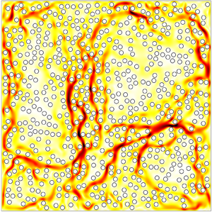With the decrease of $\phi$, the convection strength is reduced due to the enhanced drag of the porous matrix, and the temperature mixing in the bulk is less efficient, as revealed by the snapshots of the temperature and velocity magnitude in figure 1. In the presence of a small number of obstacles, the flow structure is less organized, and consequently the fluid trajectories become more irregular, as shown in figure 1(f). The flow field in porous media is highly heterogeneous due to the interaction between the porous medium and coherent flow structures, and it fluctuates both spatially and temporally. Interestingly, for small $\phi$, the flow is dominated by large-scale plumes, and convection channels with strong flow strength emerge in the pores, which are closely related to the plume dynamics, and the patches with low velocities appear due to the impedance of the obstacles (see figure 1h,k). Along the convection channels, long-range transport of fluid particles is observed, while the particles can stay ‘trapped’ for relatively long duration in the low-velocity regions. For small $\phi$, the flow exhibits columnar structures, similar to those observed in the severely confined RB convection (Chong & Xia Reference Chong and Xia2016).

Figure 1. Snapshots of (a,d,g,j) temperature $T$ and (b,e,h,k) velocity magnitude $v\equiv |\boldsymbol {v}|$, and (c,f,i,l) the typical trajectories of fluid particles for various $\phi$ at the same fluid Rayleigh number $Ra_f=10^9$: (a–c) $\phi =1$, (d–f) $\phi =0.984$, (g–i) $\phi =0.812$ and (j–l) $\phi =0.654$. In the snapshots of $v$, the obstacles are indicated by circles. In panels (c,f,i,l), the trajectories of five fluid particles are depicted, indicated by different colours. Particle positions are shown with fixed time intervals in each plot. The magnitude of particle velocity is quantified by the marker size, with larger marker for larger velocity. The integration times for the particle trajectories in panels (c,f,i,l) are 50, 80, 150 and 400 free-fall time units, respectively.

We note that the depicted flow patterns in figure 1 are robust over the time of present simulations, in the sense that, although the flow details in the pores vary with time, the global structure of flow pattern is persistent. However, in a porous medium, the statistical steady states may be different for different initial conditions. Due to the suppression of fluctuations in the presence of obstacles, the solution may not be able to sample all the flow configurations over the time range considered. As an example, we show in figure 2 two time-averaged temperature fields for the same parameters of $Ra_f=10^8$ and $\phi =0.859$, which are obtained with two different initial conditions. Despite the existence of multiple states, we expect that the differences of the statistics of multiple flow states are relatively small, and the global trend of variation of flow behaviours with porosity will not be qualitatively affected by the appearance of multiple states.

Figure 2. Time-averaged temperature fields at $Ra_f=10^8$ and $\phi =0.859$ obtained with two different initial conditions. The two solutions are persistent over at least 1000 time units, and the mean fields are obtained by averaging more than 5000 snapshots. The Nusselt numbers corresponding to panels (a,b) are 25.4 and 24.1, respectively.

The particle movement is highly irregular in the heterogeneous flow field of thermal convection in porous media. In order to quantify the chaotic particle dynamics, we plot the p.d.f.s $P(v/\sigma _v)$ of the normalized Lagrangian velocity magnitude $v/\sigma _v$ for various $\phi$ in figure 3(a), where $\sigma _v$ is the standard deviation of $v$. As $\phi$ is decreased, the shape of $P(v/\sigma _v)$ is significantly modified. With the decrease of $\phi$, the probability density for low velocity increases significantly. The time series of the normalized velocity magnitude $v/\sigma _v$ of a fluid particle are shown in figure 3(b). We find that for small $\phi$, due to the emergence of the convection channels and low-velocity regions, the time variation of $v$ exhibits strong intermittency, with the existence of high-velocity bursts, interrupted by long-time trapping events with low velocities. Similar variations of Lagrangian velocity are observed based on the other set of porous-media layout, demonstrating the robustness of the statistics with respect to the details of pore layout.

Figure 3. (a) The p.d.f.s $P(v/\sigma _v)$ of the normalized Lagrangian velocity magnitude $v/\sigma _v$ for various $\phi$, where $\sigma _v$ denotes the standard deviation of $v$. The inset shows the same data in a double logarithmic scale. (b) Typical time series of $v/\sigma _v$ for three values of $\phi$, which are indicated by the colours. From top to bottom, the porosities are 0.984, 0.906 and 0.654, respectively.

We plot in figure 4 the temporal autocorrelation function $C_v(t)=\langle [v_0-\langle v_0\rangle ][v_t-\langle v_t\rangle ]\rangle /\sigma _{v}^2$ of the particle velocity $v$ to further quantify the particle dynamics, where $v_0$ and $v_t$ indicate the velocity magnitudes at times 0 and $t$, respectively. The symbol $\langle \cdot \rangle$ denotes averaging over an ensemble of fluid particles. Results based on the two sets of random porous-media layouts are consistent. Figure 4 shows that $C_v$ decreases with $t$, demonstrating the loss of memory of the particle dynamics. Compared with the large-$\phi$ case, $C_v$ decays slower for smaller $\phi$, and the autocorrelation is enhanced with decreasing $\phi$ at fixed $t$. We note that, as $\phi$ is decreased, the decay form of $C_v$ is qualitatively changed, besides the quantitative differences in the decaying rate. For large $\phi$, the initial part of the decay process takes an exponential form, as demonstrated by the linear behaviour, $\ln (C_v)\sim t$, in the log-linear plot. For the two smallest $\phi$, the decaying behaviours of $C_v(t)$ are similar and approximately follow a stretched-exponential form with $\ln (C_v)\sim \sqrt {t}$, which suggests that the change of the velocity autocorrelation at small enough $\phi$ is attributed to the change of the characteristic time scale of Lagrangian fluid transport. The relaxation behaviour in a stretched-exponential form at small $\phi$ is attributed to the existence of very large relaxation times. To show this, the stretched exponential may be expressed as an integral of exponential functions with a spectrum of decaying rates (Johnston Reference Johnston2006; Bouchaud Reference Bouchaud2008):

(3.1)\begin{equation} \exp\left[-\left(\frac{t}{\tau}\right)^{1/2}\right]=\int_{0}^{\infty}P(\lambda)\exp\left(-\lambda\frac{t}{\tau}\right)\textrm{d}\lambda, \end{equation}

where $\tau$ denotes the characteristic relaxation time, $\lambda$ is the ratio of relaxation time and $P(\lambda )$ is the p.d.f. of $\lambda$. Smaller $\lambda$ indicates slower relaxation. Since the right-hand side of (3.1) is the Laplace transform of $P(\lambda )$, $P(\lambda )$ is obtained via taking the inverse Laplace transform. For small $\lambda$, one obtains (Johnston Reference Johnston2006)

(3.2)\begin{equation} P(\lambda)\approx \exp\left({-}B\lambda^{\beta}\right) \end{equation}

up to subleading power-law corrections, where $\beta =-1$, and $B$ is a positive constant. Expression (3.2) suggests that a very limited probability of super-slow relaxation can result in a global relaxation in a stretched-exponential form (Bouchaud Reference Bouchaud2008). The appearance of large relaxation times is attributed to the trapping events of fluid particles at low-velocity regions. The purely exponential decay corresponds to $\beta =-\infty$, i.e. no long-time relaxation (Bouchaud Reference Bouchaud2008).

Figure 4. Temporal autocorrelation function $C_v$ of Lagrangian velocity magnitude $v$ for various $\phi$. The three lines denote the fittings of the initial parts of $C_v(t)$ by an exponential function $\textrm {e}^{-at}$ (black line) and stretched-exponential function $\textrm {e}^{-\sqrt {bt}}$ (cyan and red lines) where a and b are the fitting parameters.

4. Fluid particle transport

Now we study the transport properties of fluid particles by quantifying the particle displacement $s(t)\equiv \int _{0}^{t}v(\tau )\,\textrm {d}\tau$ along the trajectory. The transport behaviours for the ensemble of particles exhibit strong fluctuations, and the ensemble-averaged displacement $\langle s\rangle$ grows with the time-independent mean velocity $\langle v\rangle$, namely, $\langle s\rangle =\langle v\rangle \cdot t$. The width of the displacement distribution is measured by the displacement variance $\sigma ^2_{s}=\langle (s-\langle s\rangle )^2\rangle$. Figure 5 shows the time evolution of $\sigma ^2_{s}$ of fluid particles for different $\phi$ at $Ra_f=10^8$ and $10^9$. It is found that $\sigma ^2_{s}$ grows ballistically with $\sigma ^2_s\sim t^2$ at small $t$. This ballistic regime is robust for different $\phi$, while the proportionality constant decreases with $\phi$. The ballistic regime is a universal phenomenon for general transport processes (Batchelor Reference Batchelor1950; Bourgoin Reference Bourgoin2015; Mathai et al. Reference Mathai, Huisman, Sun, Lohse and Bourgoin2018), and is associated with the strong Lagrangian velocity autocorrelations observed at small times.

Figure 5. Displacement variance $\sigma ^2_{s}(t)$ of fluid particles along the trajectory for various $\phi$ at $Ra_f=10^8$ and $10^9$. The values of parameters $(Ra_f,\phi )$ are given in the legend. The results at $Ra_f=10^8$ are shifted upward for clarity. The solid lines are the growth curves of $\sigma _s^2(t)$ obtained from (4.1) and the idealized velocity autocorrelation functions in exponential (black) and stretched-exponential (cyan and red) forms. For reference, several scaling laws are included as dashed grey lines.

Figure 5 also shows the deviation from the ballistic regime at large $t$, and $\sigma _s^2$ exhibits a sub-ballistic scaling, $\sigma ^2_s\sim t^{\gamma }$, with an effective scaling exponent $\gamma <2$. The transition to a different transport behaviour at large $t$ is expected and indicates the loss of memory of fluid particles to the initial conditions (Bourgoin Reference Bourgoin2015). In the presence of a small number of obstacles, due to the impact of strong velocity fluctuations, the fluid particles can efficiently explore the irregular flow field and lose the memory about the initial conditions. Consequently, the ballistic regime terminates at an early time, and beyond that the fluid particles approximately exhibit a Fickian transport behaviour with $\sigma ^2_s\sim t$, as in the case of $\phi =0.984$ in figure 5. When $\phi$ is further decreased, $\sigma _s^2$ at relatively large time displays a clear deviation from the Fickian behaviour, with an effective scaling exponent $1<\gamma <2$. This anomalous non-Fickian behaviour of particles in porous media is associated with the increased probability density of low velocity (Berkowitz et al. Reference Berkowitz, Cortis, Dentz and Scher2006; Souzy et al. Reference Souzy, Lhuissier, Méheust, Le Borgne and Metzger2020). Similar phenomena are observed for both values of $Ra_f$ considered, demonstrating the robustness for the emergence of non-Fickian behaviour with the decrease of $\phi$ in porous-media convection. Non-Fickian behaviour of particle transport is an omnipresent phenomenon and has been reported in many different settings, both with and without porous media (Richardson Reference Richardson1926; Grossmann Reference Grossmann1990; Berkowitz et al. Reference Berkowitz, Cortis, Dentz and Scher2006; Salazar & Collins Reference Salazar and Collins2009; Bijeljic et al. Reference Bijeljic, Mostaghimi and Blunt2011; Bourgoin Reference Bourgoin2015; Dentz et al. Reference Dentz, Icardi and Hidalgo2018; Puyguiraud et al. Reference Puyguiraud, Gouze and Dentz2019a, Reference Puyguiraud, Gouze and Dentzb; Souzy et al. Reference Souzy, Lhuissier, Méheust, Le Borgne and Metzger2020; Taghizadeh, Valdés-Parada & Wood Reference Taghizadeh, Valdés-Parada and Wood2020).

The transport properties of fluid particles can be related to the temporal autocorrelation function $C_v$ of particle velocity $v$, in the spirit of the Green–Kubo relations, which connect a transport coefficient to a correlation function in time (Kubo, Toda & Hashitsume Reference Kubo, Toda and Hashitsume2012). Considering that $\langle s\rangle =\langle v\rangle \cdot t$, $\sigma _s^2$ can be directly related to $C_v$ as

(4.1)\begin{align} \sigma_s^2(t)&=\langle (s-\langle s\rangle)^2\rangle=\left\langle \left(\int_{0}^{t}\,\textrm{d}t'[v(t')- \langle v\rangle]\right)^2\right\rangle \nonumber\\ &=2\sigma_v^2\int_{0}^{t}\,\textrm{d}t'(t-t')C_v(t'). \end{align}

Some derivation details are given in appendix A. Based on the numerically identified correlation behaviours in figure 4, here we consider two empirical, idealized forms of the autocorrelation function: $C_{v,1}(t)=\textrm {e}^{-at}$ and $C_{v,2}(t)=\textrm {e}^{-\sqrt {bt}}$ where a and b are the corresponding decaying rates. Here $C_{v,1}$ and $C_{v,2}$ are in the exponential and stretched-exponential forms, which are similar in form to the correlation properties of fluid particles in porous media with large and small $\phi$, respectively. Based on (4.1) and symbolic integration we obtain

(4.2)\begin{equation} \left\{\begin{aligned} & \sigma^2_{s,1}(t)=\frac{2\sigma^2_v}{a^2}(at-1+\textrm{e}^{{-}at}),\\ & \sigma^2_{s,2}(t)=\frac{4\sigma^2_v}{b^2}[bt-6+2\textrm{e}^{-\sqrt{bt}}(bt+3\sqrt{bt}+3)]. \end{aligned}\right. \end{equation}

Despite that the assumed autocorrelation functions are highly idealized, the global trend of variation of $\sigma _s^2(t)$ can be captured by (4.2), as shown in figure 5. Expressions (4.2) show that, for both forms of the velocity autocorrelation function, the particles will reach the Fickian regime in the long-time limit. The appearance of the initial ballistic regime is evident from the series expansions of (4.2) at $t=0$. When the particle velocities are exponentially correlated in time, the particles will exhibit Fickian transport behaviour for $t\gg 1/a\sim O(1)$; while when the autocorrelation function $C_v$ has a perfect, stretched-exponential form, $C_v=\textrm {e}^{-\sqrt {bt}}$, the term proportional to $\textrm {e}^{-\sqrt {bt}}$ may disrupt the appearance of the Fickian behaviour even when $t\gg 1$, resulting in the anomalous transport behaviour at relatively large $t$, consistent with the observation in figure 5. Deviations of (4.2) from the simulation results are visible, which are attributed to the deviations of the velocity autocorrelation of fluid particles from the idealized exponential or stretched-exponential forms, as shown in figure 4. Since the idealized autocorrelation functions underestimate the autocorrelation of particle velocity in porous media at large $t$ for the parameters shown, the predicted displacement variance (4.2) may fail to capture the behaviour of $\sigma _s^2$ for large times.

The above analysis shows that the anomalous transport behaviour at small $\phi$ is associated with the qualitatively different time correlation properties of fluid particles. When $t$ is large enough, the term proportional to $t$ will dominate over other terms, and the Fickian transport behaviour will be achieved (Souzy et al. Reference Souzy, Lhuissier, Méheust, Le Borgne and Metzger2020). Considering that the decaying rate of $C_v(t)$ is expected to decrease for smaller $\phi$, the preasymptotic, anomalous transport behaviour may last for relatively long time compared with the characteristic time scale of particle transport at small $\phi$, and is expected to be relevant in realistic porous-media convection.

5. Heat transfer

Now we focus on the heat transfer properties of the fluid particles. We plot in figure 6(a) the cross-correlation $C_{w,T}$ between the vertical velocity $w$ and temperature $T$ as a function of $\phi$ for fluid particles in the whole cell. We find that $C_{w,T}$ becomes significantly larger with the decrease of $\phi$. The small value of $C_{w, T}$ in the traditional RB convection is attributed to the uniform temperature distribution in the bulk with $T\approx T_m$, where $T_m$ is the arithmetic mean temperature. The large value of $C_{w,T}$ at small $\phi$ indicates that the velocity field is closely related to the motion of thermal plumes in porous-media convection, and the interaction between the porous media and thermal plumes results in the heterogeneous velocity fields. The increase of $C_{w,T}$ also reveals a remarkable mechanism to enhance the overall heat transfer of thermal convection with porous structure. As $\phi$ is decreased from 1, heat transfer enhancement is indeed observed, as shown in figure 6(b). When $\phi$ is small enough, heat transfer is reduced compared with that of traditional RB convection, which is attributed to the strong suppression of convection due to the additional drag of porous medium, as discussed in (Liu et al. Reference Liu, Jiang, Chong, Zhu, Wan, Verzicco, Stevens, Lohse and Sun2020). The anomalous transition of $Nu$ with $\phi$ around $\phi =0.764$ is associated with the change of flow organization.

Figure 6. Heat transfer statistics based on two different sets of random porous-media layouts $\text {PM}_1$ and $\text {PM}_2$. (a) Cross-correlation $C_{w,T}$ between the vertical velocity $w$ and temperature $T$ as a function of $\phi$ for fluid particles in the the whole cell at $Ra_f=10^8$ and $10^9$. The inset shows the typical time series of the convective heat flux $w\cdot \delta T$ in the vertical direction (red lines) and $w$ (blue lines) based on $\text {PM}_1$ at $Ra_f=10^9$ and various $\phi$: from top to bottom $\phi =1$, $0.984$ and $0.812$, corresponding to the filled symbols in the $C_{w,T}(\phi )$ plot. (b) The normalized Nusselt number $Nu/Nu(1)$ as a function of $\phi$ for $Ra_f=10^8$ and $10^9$.

The inset of figure 6(a) shows the time series of the convective heat flux $w \delta T$ in the vertical direction and the vertical velocity $w$ of fluid particles for various $\phi$, where $\delta T=T-T_m$. In the traditional RB convection with $\phi =1$, the fluid particles with high velocity may not contribute to the vertical heat transfer for relatively long times, which is due to the fact that the temperature in the centre core is well mixed with small temperature fluctuation $\delta T$; while for small $\phi$, the low amplitude of the vertical heat transfer is mainly due to the low particle velocity, confirming the strong cross-correlation between the vertical velocity and temperature fluctuation. As a consequence of this enhanced cross-correlation, the probability of negative Lagrangian heat transfer in the bulk region will be decreased compared with that in the traditional RB convection.

The pore-scale Péclet number $Pe=vD/\kappa$ quantifies the ratio of the thermal diffusion time scale $\tau _{\kappa }=D^2/\kappa$ to the convection time scale $\tau _c=D/v$, where $v$ is the fluid velocity, $D$ the obstacle diameter and $\kappa$ the thermal diffusivity. In dimensionless form, we have $\kappa =1/\sqrt {PrRa_f}$. In the convection channels with fast fluid transport, $Pe$ is high, and in the low-velocity regions, $Pe$ is low. For the Rayleigh numbers considered, $Pe$ is generally larger than 1 (except at the stagnant regions with very low velocities). For $Ra_f=10^9$, the peak value of $Pe$ is of order $O(100)$ at small porosities. The Péclet number has important implications to the temperature evolution. A large $Pe>1$ indicates that the transport of temperature is dominated by convection rather than diffusion, such that there may not be enough time for the obstacles to respond to the temperature fluctuations, which may result in a less uniform temperature distribution across the fluid–solid interface. A larger $Pe$ (stronger convection) will also result in more efficient convective mixing. As an example, we depict in figure 7 the instantaneous temperature distributions for $Ra_f=10^8$ and $10^9$ at $\phi =0.812$. It is found that the bulk temperature for larger $Ra_f$ (larger $Pe$) is closer to the arithmetic mean value $T_m=0.5$, demonstrating the more efficient temperature mixing for larger $Ra_f$. When the bulk flow is sufficiently mixed, one would expect a uniform temperature distribution with $T\approx T_m$, as shown in figure 1(a). Figure 7 also shows that for larger $Ra_f$ the temperature across the fluid–solid interface is less uniform, as manifested by the more evident imprint of the solid phase in figure 7(b).

Figure 7. Instantaneous temperature distributions at (a) $Ra_f=10^8$ and (b) $Ra_f=10^9$ at $\phi =0.812$.