


1. Introduction
Irrotational periodic deep-water surface waves have particle trajectories that are not closed but open, leading to a relatively weak mass transport in the direction of wave propagation, known as Stokes drift (Stokes Reference Stokes1847; Kenyon Reference Kenyon1969). When waves break, they can rapidly transport mass near the surface of the water (Deike, Pizzo & Melville Reference Deike, Pizzo and Melville2017; Lenain, Pizzo & Melville Reference Lenain, Pizzo and Melville2019; Pizzo, Melville & Deike Reference Pizzo, Melville and Deike2019). While the former effect is classical, the latter has only recently been quantified, and many questions remain concerning the behaviour of the breaking-induced flow. In particular, Lenain et al. (Reference Lenain, Pizzo and Melville2019) hypothesized that packet bandwidth plays an important role in modulating the surface transport induced by breaking. In this paper, we corroborate this hypothesis and propose a scaling argument to explain and model these findings.
The surface transport due to wave breaking plays an important role in upper ocean processes. For instance, the surface vertical vorticity (Melville, Veron & White Reference Melville, Veron and White2002; Pizzo & Melville Reference Pizzo and Melville2013) induced by deep-water wave breaking (due to the finite crest length of these breaking events), together with the Stokes drift, generates Langmuir circulations through the so-called type 2 Craik-Liebovich (CL2) mechanism (Leibovich Reference Leibovich1983). These circulations generate a vertical flux of horizontal momentum, mixing the upper ocean and modulating the thermal boundary condition between the atmosphere and the ocean (McWilliams, Sullivan & Moeng Reference McWilliams, Sullivan and Moeng1997; Sullivan, McWilliams & Melville Reference Sullivan, McWilliams and Melville2004), a crucial boundary condition for coupled air–sea models (Belcher et al. Reference Belcher2012; Li et al. Reference Li, Webb, Fox-Kemper, Craig, Danabasoglu, Large and Vertenstein2016). However, current parameterizations of these processes do not take wave breaking into account, even though there is numerical evidence (Sullivan, McWilliams & Melville Reference Sullivan, McWilliams and Melville2007) that breaking can strongly modify the mixed layer dynamics. Furthermore, there is practical value in modelling the advection of flotsam, jetsam and pollution at the surface of the ocean (van den Bremer & Breivik Reference van den Bremer and Breivik2018).
Deike et al. (Reference Deike, Pizzo and Melville2017) used direct numerical simulations of a two phase air–water system to examine the mass transport induced by deep-water breaking waves. In that study, the authors proposed a simple model for the surface transport induced by breaking, finding (based on theoretical work on the particle kinematics near breaking described in Pizzo Reference Pizzo2017) that the surface transport scales linearly with  $S$, where
  $S$ is a measure of the wave slope, whereas the classical Stokes drift scaled like
  $S^2$ (note,
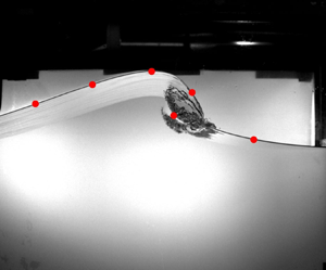
  $S<1$). Pizzo et al. (Reference Pizzo, Melville and Deike2019) then used this model, together with the statistics of wave breaking at sea, to estimate the total surface transport induced by wave breaking, finding that, for the sea states considered there, the surface transport induced by breaking may be up to 30 % of the Stokes drift. Subsequently, Lenain et al. (Reference Lenain, Pizzo and Melville2019) conducted laboratory experiments on the surface transport due to breaking, and found agreement with the numerical studies. Furthermore, the authors examined and elucidated the spatial dependence of the surface transport induced by breaking. In setting up these experiments, the authors noticed that packet bandwidth seemed to modify the breaking transport (see figure 1), but did not seek to quantify this effect in their study.

Figure 1. Particle transport for two breaking wave packets of similar slope, but different bandwidths, in a laboratory experiment. The breaking packet was travelling from left to right. The colours indicate time (blue/green is an earlier time than orange/red). The trajectories of these quasi-neutrally buoyant particles cannot be tracked during active air entertainment, which explains the gap in particle locations. The top packet has a larger bandwidth than the bottom packet. We see that the particle in the narrower banded wave packet travels significantly further than that in the broadband packet. Quantifying this difference is the motivation for this paper.
Breaking waves in the laboratory may be generated using a dispersive focusing technique, in which the relative phases of longer faster waves and shorter slower waves are tuned so that, according to linear theory, the waves constructively interfere at a point in space and time (Longuet-Higgins Reference Longuet-Higgins1974; Rapp & Melville Reference Rapp and Melville1990). This is believed to model an important source of breaking in deep water, in which the dispersive waves in a broadband sea state constructively interfere at random, leading to wave breaking (Rapp & Melville Reference Rapp and Melville1990). Linear broadband wave packets are generated and measured far upstream and downstream of the focusing event. Furthermore, quantities of interest are directly measured in the breaking region. Then, models that relate the behaviour of the breaking-induced flow to the initial conditions of the system may be validated, allowing for the testing of predictive models of the behaviour of breaking waves.
Through a series of publications, it has been shown that variables characterizing these focusing wave packets set the scales for properties of the breaking-induced flow. This includes the energy dissipation rate due to breaking (Drazen, Melville & Lenain Reference Drazen, Melville and Lenain2008; Tian, Perlin & Choi Reference Tian, Perlin and Choi2010; Romero, Melville & Kleiss Reference Romero, Melville and Kleiss2012; Grare et al. Reference Grare, Peirson, Branger, Walker, Giovanangeli and Makin2013; Perlin, Choi & Tian Reference Perlin, Choi and Tian2013), the mean flow induced by breaking (Pizzo & Melville Reference Pizzo and Melville2013, Reference Pizzo and Melville2016) and the volume of air entrained by breaking (Deike, Melville & Popinet Reference Deike, Melville and Popinet2016). Note, many of these scaling laws have also been corroborated by numerical experiments (Deike, Popinet & Melville Reference Deike, Popinet and Melville2015; Deike et al. Reference Deike, Melville and Popinet2016; Derakhti & Kirby Reference Derakhti and Kirby2016). In these studies the independent variable used to scale these properties was  $S$, the linear prediction of the maximum wave slope at focusing. In broadband packets, this has been shown to correlate well with
  $h$, the height of the wave at breaking, which is the relevant length scale for characterizing the energy dissipation (Duncan Reference Duncan1981, Reference Duncan1983; Drazen et al. Reference Drazen, Melville and Lenain2008). However, there was uncertainty in how to scale the width of the breaking region and the duration of breaking, and for simplicity these were assumed to scale with the central frequency and wavenumber (Rapp & Melville Reference Rapp and Melville1990; Drazen et al. Reference Drazen, Melville and Lenain2008; Tian et al. Reference Tian, Perlin and Choi2010). In the context of the energy dissipation, this was acceptable, as the slope dependence changed the dissipation rates by nearly three orders of magnitude, while the scatter in the duration of breaking implied a factor of two difference across that parameter regime. However, when establishing the surface transport induced by breaking, a factor of two becomes critically important as the values of the drift tend to only vary over one order of magnitude. Therefore, these corrections are significant in judging the importance of wave breaking vs other sources of transport at the ocean surface.
In this paper, we have conducted laboratory experiments examining focusing deep-water wave packets. The trajectories of quasi-neutrally buoyant particles were examined both for breaking and non-breaking events. Particle positions before and after the passing of the wave packet were manually identified from images taken by an overlooking camera, and the bulk horizontal Lagrangian transport was computed. The packet bandwidth and slopes were varied. A scaling argument is proposed, which predicts the width of the breaking region, and this model is corroborated by the laboratory data. Finally, we employ the new scaling relationship for the width of the breaking region to update the existing model of the wave-breaking dissipation rate (Drazen et al. Reference Drazen, Melville and Lenain2008).
In § 2 the experimental set-up is described. In § 3 the measurements of Lagrangian transport are presented. In § 4 a scaling argument is provided that leads to a model of the horizontal length scale of breaking, along with a model of the mean transport by breaking waves. These models are corroborated in § 5, and improvements to the model of the dissipation rate are discussed in § 6. Finally, in § 7 we present our conclusions.
2. Experiments
2.1. Facilities
The experiments were conducted at the rebuilt (2017) Glass Channel Facility in the Hydraulics Laboratory at the Scripps Institution of Oceanography (SIO). The stainless steel and glass tank (see figure 2a) is 32 m long, 0.5 m wide and 1 m deep. Wave packets were generated using a computer-controlled electro-mechanical wave maker installed at one end, while a beach of  $9^{\circ }$ slope, covered with a thick fibrous mat, was installed on the other end, to absorb and dissipate any waves that reached the end of the channel, minimizing wave reflections. Each run corresponded to the generation and measurement of a single wave packet. The tank was filled with fresh water to a working depth of 0.50 m.

Figure 2. Diagram of the experimental set-up. (a) Conceptual diagram of the wave tank, including location of the breaking region and the seven wave gauges. (b) Close-up of the breaking region. In these experiments, the measured trajectories of 18 nearly neutrally buoyant particles were used to estimate the total surface transport induced by focusing non-breaking and breaking wave packets. The images used to measure particle displacement were taken with the downward-looking camera. The side-looking camera was used to measure wave height at breaking ( $h$) and to obtain the breaking locations
  $x_b$. A hydrophone (not pictured) was used to measure the active breaking duration for the breaking packets and was located at the bottom of the tank, roughly
  $50\ \text {cm}$ down-channel from the breaking location.
Note, throughout this paper we will make use of the archived data from Lenain et al. (Reference Lenain, Pizzo and Melville2019), which, when necessary to distinguish, we denote as LPM, while the data from this experiment are denoted SGLP. Wave packet spectral parameters and measurements for these experiments are provided in table 1.
Table 1. Table of wave packet spectral parameters and measurements;  $f_c$ is the packet centre frequency,
  $\varDelta$ is the corresponding bandwidth,
  $S_*$ is the breaking threshold,
  $S$ is the slope,
  $h$ is the wave height at breaking,
  $c_{gs}$ is the spectrally weighted group velocity,
  $\delta F_b$ is the energy flux lost due to breaking,
  $\tau$ is the duration of active breaking,
  $b$ is the breaking dissipation,
  $x_{02}-x_{01}$ is the width of the averaging window used when calculating the net surface transport and
  $\langle \overline {\delta x}\rangle$ is the mean surface transport.

2.2. Focusing packet generation
The wave packets were generated using a dispersive focusing technique. That is, by exploiting the fact that longer waves travel faster than shorter waves in deep water, and tuning the relative phases of the packet components, focusing packets may be created (Longuet-Higgins Reference Longuet-Higgins1974; Rapp & Melville Reference Rapp and Melville1990).
Following Drazen et al. (Reference Drazen, Melville and Lenain2008), in these experiments we generate wave packets of the form
 \begin{equation} \eta(x,t) = \sum_n^N a_n\cos(k_n(x-x_b)-\omega_n(t-t_b)), \end{equation}
where  $a_n$ are the amplitudes of the
  $N$ Fourier components, and
  $k_n$ and
  $\omega _n$ are their wavenumbers and radial frequencies, respectively, related by the dispersion relation
  $\omega _n^2 = gk_n\tanh (k_nd)$ in water of depth
  $d$, where g is gravitational acceleration. The variables
  $x_b$ and
  $t_b$ are the prescribed focusing location and time, respectively, as predicted by linear theory. Thus, according to (2.1), all of the components constructively interfere at
  $(x_b,t_b)$. Furthermore, the wave train described by (2.1) is windowed, so that only one wave packet is generated.
Furthermore, the spectrum of the wave packet is localized in frequency space, so that it has a well-defined bandwidth and central frequency  $f_c$. The normalized bandwidth
  $\varDelta$ is defined as
 \begin{equation} \varDelta \equiv \frac{f_N-f_1}{f_c}, \end{equation}
so that the dimensionful bandwidth  $f_c\varDelta$ contains all of the Fourier components which contribute to the wave packet at focusing. Note, the definition presented in (2.2) assumes that the spectral distribution is uniform.
2.3. Surface elevation and hydrophone measurements
The height of the free surface  $\eta (x,t)$ was measured with seven resistance wire wave gauges placed along the channel at positions 1.76, 4.76, 5.38–7.76, 13.76, 15.76, 17.76 and 19.76 m from the mean position of the wave paddle. (The third wave gauge was moved upstream in some cases to avoid being near the breaking location of the narrow-banded packets). The wave gauge signals were subsequently amplified using an amplifier from the Danish Hydraulics Institute (Model 80-74G) and digitized. Furthermore, we conducted experiments in which no particle locations were measured, but instead we recorded the duration of active breaking
  $\tau _{br}$, which was estimated from the acoustic signal of the breaking event, measured by an hydrophone placed at the bottom of the tank.
2.4. Surface transport measurements
To measure the surface transport, the surface of the water was seeded with 18 slightly buoyant coloured particles of  $11.8\ \text {mm} \pm 0.1\ \text {mm}$ diameter. The size of the particles was chosen for their visibility before and after breaking, and because they should follow the flow streamlines without excessive slip (Melling Reference Melling1997). The mass densities of the particles were calculated from their buoyant forces. Buoyancy was measured by releasing the particles at depth in a small tank filled with water at rest and recording their rise velocities with a high-speed camera (Model Phantom M320s), giving a mean particle material density of
  $0.9960\ \text {g}\ \text {cm}^{-3}$ with a maximum density of
  $0.9974\ \text {g}\ \text {cm}^{-3}$ and a minimum density of
  $0.9937\ \text {g}\ \text {cm}^{-3}$. Starting at rest and at depth, the particles were observed to rise at speeds
  $O(10^{-2})\ \text {m}\ \text {s}^{-1}$ (with corresponding Reynolds number
  $O(10)$). Typical speeds observed during breaking are
  $O(1)\ \text {m}\ \text {s}^{-1}$ (Rapp & Melville Reference Rapp and Melville1990; Melville et al. Reference Melville, Veron and White2002; Drazen & Melville Reference Drazen and Melville2009). Therefore, the magnitudes of particle rise velocities are small in comparison with the speed of the flow near the surface at breaking, so we expect the effects due to buoyancy to negligibly affect the particle trajectories during breaking.
The particles were painted to distinguish between them, but to accommodate 18 particles, some colours were repeated. Particles of the same colour were placed sufficiently far apart to distinguish them.
Before the wave packet was generated, the particles were released and remained at rest almost completely submerged. The wave maker generated a wave packet and two cameras placed near the breaking region were simultaneously triggered. A downward-looking camera, mounted above the channel, took pictures at a prescribed sampling frequency, and was used to record the particle locations before and after the passing of the wave packet. A side looking camera was used to identify the location of maximum focusing  $x_b$, and, in the case of wave breaking, to measure the height of the breaking wave
  $h$. The cameras sampled for less than one minute, while the wave gauges sampled for three minutes. After the wave gauges stopped recording, the channel was left undisturbed for 12 min to allow time for the water to come to a state of rest, at which point the next run was conducted.
This operation was repeated with the initial positions of the particles being moved upstream and downstream of the breaking location so that the Lagrangian transport was measured across the entire region of significant transport.
2.5. Imagery
Images of the breaking region were taken with two colour cameras (see figure 2b): a downward-looking camera and a side-looking camera. The downward-looking camera was a Nikon D810 SLR ( $7360 \times 4912\ \textrm {px}$,
  $35.9 \times 24 \ \text {mm}$ full frame FX format CMOS sensor with
  $4.88\ \mathrm {\mu }\text {m}$ pixel size) that was mounted above the channel and equipped with a 14 mm
  $f/$2.8
 $D$ Nikon lens. The camera took
  $104$ images per run, sampling at
  $3\text { Hz}$ for the first 80 images, followed by an image every
  $600\ \text {ms}$ for the remaining 24 images. The side-looking camera was a JaiPulnix AB800CL colour camera (
 $3296 \times 2472\ \textrm {px}$,
  $18.13 \times 13.6\ \text {mm}$ 4/3 inch format CCD with
  $5.5\ \mathrm {\mu }\text {m}$ pixel size) with a
  $14\ \text {mm}$
  $f/$2.8
 $L$ Canon lens. This camera sampled at 10 Hz. The camera was placed adjacent to the channel and pointed at the wave-breaking region.
3. The variables of surface transport
3.1. Characteristic wave variables
Following Rapp & Melville (Reference Rapp and Melville1990), we characterize the focusing wave packets through the linear prediction of the maximum slope at focusing  $S$, the normalized bandwidth
  $\varDelta$, the central frequency
  $f_c$ and the focusing location according to linear theory
  $x_b$. In this study we examine the effects of the two variables
  $S$ and
  $\varDelta$ on surface transport.
3.2. The linear prediction of the maximum slope,  $S$ and the wave packet bandwidth, $\varDelta$


The strength of focusing or breaking is measured with the quantity  $S$, the linear prediction of the maximum slope at focusing, (which we also refer to as the slope) and has been traditionally equated with a sum of the slopes
  $\sum _n a_nk_n$ of the Fourier components in (2.1). This parameter corresponds qualitatively to the strength of the breaking event, with larger
  $S$ generally implying a stronger breaking event, which is characterized by a greater wave height at breaking
  $h$ (the definition of which is illustrated in figure 1(b) of Drazen et al. Reference Drazen, Melville and Lenain2008).
Following Tian et al. (Reference Tian, Perlin and Choi2010), we seek to measure this quantity, instead of using the a priori prescribed value, in order to avoid any assumptions regarding the transfer function of our wave paddle. As was noted by Tian et al. (Reference Tian, Perlin and Choi2010), the sum  $\sum _n a_n k_n$ of the Fourier coefficients at the first wave gauge does not converge due to the amplification of the shorter wave components. This is remedied by excluding Fourier components that lie outside of the bandwidth
  $f_c\varDelta$.
The bandwidth was determined by minimizing the  $L_2$ norm of the difference between the measured and the linear prediction of free surface displacement at wave gauges 2 and 3 (which were chosen because they are upstream of the breaking location). The linear prediction was computed by propagating the free surface measured at the first wave gauge and band-pass filtered using a window of width
  $f_c \varDelta$ centred on
  $f_c$. The bandwidth was increased until this metric reached a constant value. Note that the bandwidths described using this method were such that, on average, they contained
  $95.9\pm 1.8\,\%$ of the total wave packet energy measured at wave gauge 1. Furthermore, the computed bandwidths are linearly proportional to the prescribed bandwidth values.
Because excluding the Fourier components that lie outside of our computed bandwidths improves the accuracy of the linear prediction of the free surface upstream from the breaking location, it will also improve our estimates of the slope at focusing  $S$. Therefore, the slope is defined as
 \begin{equation} S \equiv \max(|\eta_{x}(x,t)|), \end{equation}
where  $\eta (x,t)$ is the linear prediction of the free surface displacement and
  $\eta _{x}(x,t)$ is its spatial derivative. The linear prediction of the free surface displacement was computed from the spectral and phase information of the band-passed wave packet measured at the first wave gauge. The surface displacement and its spatial derivative were computed with a spatial resolution of
  $1\ \text {cm}$, which is small enough to accurately estimate
  $S$.
$S$.
The most important test of our estimates of the slope is its relationship with the wave height at breaking  $h$, which is shown in figure 3. The slope is a measure of the strength of breaking, and its correlation with the wave height at breaking is the motivation for its use in these experiments. In that figure, it is shown that the linear prediction of the maximum slope scales approximately linearly with
  $hk_c$, so that this parameter
  $S$ characterizes the breaking strength. For comparison, figure 15 of Drazen et al. (Reference Drazen, Melville and Lenain2008) also compares prescribed
  $S$ values with direct video measurements of
  $hk_c$. They also observed a linear relationship, but with significantly more scatter. This implies that our method of estimating
  $S$ provides a more accurate description of the breaking region than the prescribed values. We also note that, while each data point on that figure in Drazen et al. (Reference Drazen, Melville and Lenain2008) represents a single direct video measurement, each data point in figure 3 of this paper represents the mean of 50 to approximately 150 direct video measurements.

Figure 3. The dimensionless wave height  $hk_c$ plotted against the linear slope at focusing
  $S$ minus the breaking threshold value
  $S_*$. The black line is a best fit of the form
  $hk_c = \chi _h(S-S_*)$, where
  $\chi _h$ is a fitting constant equal to 4.15. There is no significant effect of the bandwidth on the relationship between
  $hk_c$ and the slope
  $S$, save for through the weak dependence of
  $S_*$ on
  $\varDelta$, which is accounted for by our choice of the independent variable as
  $S-S_*$. This figure includes data from LPM (triangles) and SGLP (circles).
Wave packets with  $S$ values slightly above a breaking threshold
  $S_*$ exhibit spilling breaking, and as
  $S$ increases, the packets transition to plunging breakers or multiple breakers. In this study, only single breaking events are considered. Note, we define the breaking threshold as the value
  $S_*=S$ when the free surface first entrains air, as detected by the side-looking camera. The breaking threshold values are given in table 1 and shown in figure 9.
Note, in § 6 we consider archived data from Drazen et al. (Reference Drazen, Melville and Lenain2008), and recompute their values of  $S$ and
  $\varDelta$ using the definitions given in this section.
3.3. Surface transport measurements
Figure 4 shows measurements of the surface Lagrangian transport  $\delta x$ computed from particle displacements as a function of the distance from the breaking location
  $(x_0-x_b)$ where
  $x_0$ is the initial position of the particle and
  $x_b$ is the measured breaking location (this is the location where the free surface first becomes multi-valued) of the wave packet. The figure is organized into panels by the bandwidth and the data points are colour coded by the slope
  $S$. Each panel in figure 4 contains all the Lagrangian transport measurements of each run for a given bandwidth and central frequency. Every data point in these figures corresponds to a single particle displacement.

Figure 4. Lagrangian transport  $\delta x$ as a function of the initial distance from the breaking location,
  $(x_0-x_b)$. Each point corresponds to a single particle displacement. Each panel presents data from packets with the same bandwidth
  $\varDelta$ and central frequency
  $f_c$; data points are colour coded by slope
  $S$;
$S$;  $x_b$ is defined as the location where the free surface becomes vertical. For non-breaking packets, the breaking location
  $x_b$ of the lowest
  $S$ single breaking packet is used.
The Lagrangian transport is noticeably asymmetric, with the maximum of the transport located close to the breaking location  $x_b$. It is sharply peaked for packets with higher
  $S$ and
  $\varDelta$ values. The low transport values slightly downstream of
  $x_b$ in figures 4(b) and 4(d) correspond to particles that have been pushed downward into the water column by energetic plunging breakers. The slopes of the breaking wave packets with bandwidths
  $\varDelta = 0.77$ and
  $\varDelta = 0.91$ were in the range
  $0.32 - 0.33$ and
  $0.38 - 0.41$, respectively, while the slopes of breaking wave packets with bandwidths
  $\varDelta = 1.05$ and
  $\varDelta = 1.15$ were in the range
  $0.30 - 0.39$, and
  $0.38 - 0.46$, respectively. The narrowness of the range of breaking slopes measured in the two smaller bandwidth wave packets is due to the technical limitations of generating steep wave packets with narrow bandwidths in a wave tank of finite length. Wave packets with small bandwidth need more distance to focus and de-focus than packets with larger bandwidth. To counteract this effect, for small bandwidths, packets with large slope values must be generated with an initial large steepness which can violate our assumption that the wave field is linear at the first wave gauge. Therefore, the initial steepness of the small bandwidth wave packets has been limited, reducing the range of S values for these breaking packets.
In figure 5, the averaged surface Lagrangian transport  $\overline {\delta x}$ for each slope and bandwidth combination is shown. The averaged Lagrangian transport
  $\overline {\delta x}$ is computed by averaging the Lagrangian transport
  $\delta x$ over a running window as follows:
 \begin{equation} \overline{\delta x}(x_0) = \frac{4}{\lambda_c}\int_{x_0-\lambda_c/8}^{x_0+\lambda_c/8} \delta x(\tilde{x}) \,\text{d}\tilde{x}, \end{equation}
where  $\tilde {x}$ is a dummy variable. This is the same method as employed in Lenain et al. (Reference Lenain, Pizzo and Melville2019).

Figure 5. Averaged Lagrangian transport  $\overline {\delta x}$ as a function of the distance from the breaking location, both variables being normalized by the central wavenumber
  $k_c$. The averaged Lagrangian transport
  $\overline {\delta x}$ is defined in (3.2). Each panel presents data from packets with the same
  $\varDelta$ and
  $f_c$. The breaking location
  $x_b$ is the same as in figure 4. The effect of
  $S$ on both the amplitude of the transport and the width of the breaking region is clearly illustrated here, particularly in (c,d), as increasing
  $S$ noticeably increases both of these values. Qualitative differences in the shape of the average transport curves is noticeable between wave packets with different bandwidths but similar
  $S$ values, implying that the Lagrangian transport depends both on
  $\varDelta$ and
  $S$. (Note, the sudden increase in average transport far downstream from the breaking region in panel (b) is caused by four data points (visible in figure 4b), so we do not consider it statistically significant.)
In figure 5 the dependence of the mass transport on the slope is apparent, and some effects of the bandwidth can be seen. Within figures 5(c) and 5(d), greater average transport and wider regions of significant breaking-induced transport are observed in steeper wave packets. There are also qualitative differences observed between breaking wave packets with different bandwidths but similar slopes. For instance, in figure 5(b), the averaged surface transport  $\overline {\delta x}(x_0)$ of the breaking packets generally decrease monotonically from their maxima. The slope values are ranging from
  $S=0.38$ to
  $S=0.41$. In figure 5(c), the curve showing the averaged transport profile of the wave packet of the highest slope
  $S=0.39$ has two maxima separated by a distance of roughly 7 radians (i.e. approximately 2 m).
To illustrate the effects of bandwidth on the average transport, the average transport curves of two wave packets of similar slope and differing bandwidths are plotted in figure 6. From this figure, it can be seen that an increase in the bandwidth  $\varDelta$ corresponds to a decrease in the width of the region of significant breaking-induced transport, as well as a decrease in the average transport.

Figure 6. Averaged Lagrangian transport  $\overline {\delta x}$ of two wave packets with similar slopes but different bandwidths. The average transport and the width of the region of significant breaking-induced transport are observed to decrease as the bandwidth is increased. Both axes are normalized by the central wavenumber
  $k_c$, which is the same for both of the wave packets in this figure.
To estimate the overall surface transport induced by the passing of a wave packet, we define the mean surface transport  $\langle \overline {\delta x}\rangle$ as the integral of the averaged surface transport
  $\overline {\delta x}$ over the region of significant transport, the limits of which are denoted
  $x_{01}$ and
  $x_{02}$, such that
 \begin{equation} \langle\overline{\delta x}\rangle \equiv \frac{1}{x_{02}-x_{01}} \int_{x_{01}}^{x_{02}}\overline{\delta x}(x_0)\,\text{d}\kern0.7pt x_0. \end{equation}
The limits of the region of significant transport are defined as the first points upstream and downstream of the breaking location where the average transport curve becomes flat.
4. The length scale of the mean drift induced by wave breaking
In this section we seek to constrain the horizontal length scale associated with wave breaking. Breaking surface gravity waves are unsteady in time and vary in space. Several laboratory experiments aimed at quantifying this unsteadiness have been conducted. This includes Rapp & Melville (Reference Rapp and Melville1990), who used dye to quantify the breaking area (see their figures 32 and 33), although they were more interested in long time asymptotic behaviour. Next, Drazen et al. (Reference Drazen, Melville and Lenain2008) used a hydrophone to measure the temporal duration of active breaking by using an intensity threshold criterion. Tian et al. (Reference Tian, Perlin and Choi2010) measured the width of the active breaking region, which they defined as the distance between the point where the free surface becomes vertical and where the front of the breaking crest ends and the generation of the bubble cloud associated with breaking stops.
Here, we define the length scale of the breaking-induced mean transport to be the region over which significant mass transport occurs. This definition arises naturally from the form of the breaking-induced drift distributions which are strongly peaked (refer to figure 5).
To constrain this length scale, we consider a simple model for wave breaking, motivated by the turbulent gravity current arguments of Longuet-Higgins & Turner (Reference Longuet-Higgins and Turner1974). In particular, we associate wave breaking with the exceedance of a steepness threshold (Perlin et al. Reference Perlin, Choi and Tian2013), which triggers a local crest instability (Longuet-Higgins & Fox Reference Longuet-Higgins and Fox1977), that is analogous to the superharmonic instability of Stokes waves (Longuet-Higgins Reference Longuet-Higgins1978; McLean Reference McLean1982). These instabilities then lead to large geometrically driven horizontal accelerations near the crest (Vinje & Brevig Reference Vinje and Brevig1981; Pizzo Reference Pizzo2017). This leads to wave overturning and free surface re-connection (which topologically changes the fluid and introduces vorticity into the bulk of the fluid – see Hornung, Willert & Turner Reference Hornung, Willert and Turner1995; Pizzo & Melville Reference Pizzo and Melville2013).
The re-connection of the free surface entrains air into the water, forming an air–water mixture. This mixture then rides down the forward face of the wave group, in a manner similar to what was described in Longuet-Higgins & Turner (Reference Longuet-Higgins and Turner1974). This is sustained as long as the free surface is steep enough that the gravitational acceleration of the plume exceeds the deceleration due to friction between it and the free surface. Therefore, this process is governed by a slope threshold, so that the width of this region may be found by knowledge of a function  $f$, defined as
 \begin{equation} f(x) \equiv {\rm max}_t(|\eta_x|), \end{equation}
where  $\text {max}_t$ is the maximum taken over time, such that
  $f(x)$ still has
  $x$ dependence. Therefore
  $f(x)$ represents the maximum slope the linear prediction of the free surface achieves at each point in the wave channel.
We know that  $f(x)$ reaches a maximum value
  $S$ near the point
  $x_b$ and that, in the breaking cases,
  $f(x)$ equals the breaking threshold slope
  $S_*$ at two points on either side of this critical point. By taking a local second-order Taylor expansion about the maximum of
  $f(x)$, we may define the length scale
  $L$, which is given by the width of the region where
  $f(x)>S_*$. That is, we define
 \begin{equation} L \equiv 2(x_*-x_b), \end{equation}
where  $x_*$ is the location where
  $f(x)$ passes below
  $S_*$.
Following the arguments presented in Fedele (Reference Fedele2014), it may be shown that for narrow-banded wave packets the length scale associated with the focusing event is given by
 \begin{equation} k_cL = \frac{\gamma}{\varDelta}\sqrt{S-S_*}, \end{equation}
where  $\gamma$ is a scaling constant. We recall that our hypothesis is that the mean surface transports scales linearly with this quantity, so that
 \begin{equation} k_c\langle\overline{\delta x}\rangle =\frac{\chi}{\varDelta}\sqrt{S-S_*}, \end{equation}
for  $\chi$ another scaling constant.
It is worth noting that, although the argument that leads to (4.4) assumes that value of the maximum slope is symmetric about its critical point, the averaged Lagrangian transport  $\overline {\delta x}$ may still be asymmetric. To see this, consider a simple model of the transport, in which the particles are transported from their initial location in the breaking region to the end of the breaking region
  $x_*$. Therefore, the particles initially located at the beginning of the breaking region are transported the greatest distance, as they traverse the entire width of the breaking region
  $L$. Then, this predicts that
  $\overline {\delta x}(x_0)$ takes the form of a right triangle, with maximum value
  $L\chi / \gamma$. In reality, the averaged Lagrangian transport takes on a more complicated spatial dependence than this model, but this approach serves as a useful way of qualitatively interpreting figure 5.
5. Results
In this section we present our measurements of the mean surface transport  $\langle \overline {\delta x}\rangle$, and subsequently compare it with the predictions of our scaling arguments.
In figure 7, the measurements of the mean surface transport  $\langle \overline {\delta x}\rangle$ are presented, first scaled using only the central wavenumber
  $k_c$ and plotted against the slope
  $S$ in (a), then scaled with the bandwidth
  $k_c \varDelta$ and plotted against the slope subtracted by the breaking threshold slope
  $S-S_*$ in (b). In figure 7(a), the mean surface transport of wave packets with different bandwidths follow distinctly different curves both in the breaking and non-breaking cases. Also apparent is the significant increase in the mean surface transport induced by breaking compared with non-breaking packets, as was observed in Deike et al. (Reference Deike, Pizzo and Melville2017) and Lenain et al. (Reference Lenain, Pizzo and Melville2019). Figure 7(b) shows that using the length scale
  $(k_c \varDelta )^{-1}$ and using
  $S-S_*$ as the independent variable collapses the measurements of
  $\langle \overline {\delta x}\rangle$ onto a curve with functional form
 \begin{equation} \langle\overline{\delta x}\rangle k_c\varDelta = \chi_l \sqrt{S-S_*}+\beta. \end{equation}
Note, the window length  $x_{01}-x_{02}$ as a function of
  $S$ is shown in the Appendix in figure 14.

Figure 7. Measurements of the mean transport  $\langle \overline {\delta x}\rangle$ induced by breaking (diamonds) and non-breaking (circles) focusing wave packets. In (a),
  $\langle \overline {\delta x}\rangle$ is normalized using the central wavenumber
  $k_c$ and plotted against
  $S$. In (b),
  $\langle \overline {\delta x}\rangle$ is normalized by
  $k_c \varDelta$ and plotted as a function of
  $S-S_*$; the solid black line is a fit of the form
  $\langle \overline {\delta x}\rangle k_c\varDelta = \chi _l\sqrt {S-S_*}+\beta$ where
  $\chi _l = 7.39$ and
  $\beta = 0.69$. Here,
  $\beta$ is not a free parameter, but is the measurement of the maximum non-breaking surface drift, normalized by the bandwidth and central wavenumber. In (a), data from the four different bandwidths lie on different curves, both for the breaking and non-breaking cases. It is clear that
  $k_c$ and
  $S$ alone do not set the mean transport induced by breaking, while
  $k_c \varDelta$ accounts well for the dependence of the mean transport on bandwidth. Furthermore, measurements of the breaking transport agree well with the scaling arguments developed in § 4. This figure includes data from LPM (
 $\varDelta = 1.05$) and SGLP (other
  $\varDelta$ values).
The data collapse is mostly attributed to the use of  $(k_c\varDelta )^{-1}$ as the length scale of the mean transport. The vertical offset
  $\beta$ is not a free parameter. The value of
  $\beta$ used in this paper is the maximum bandwidth-normalized surface transport measured for non-breaking wave packets. Because the bandwidth and central frequency are taken into account in our scaling,
  $\beta$ does not vary between wave packets with different bandwidths or central frequencies, and it is found to have a value of
  $0.69$ in this study. See also figure 11, which illustrates the role of the breaking threshold in the scaling.
There are two notable developments in this result which have not been observed before. First, the inverse dependence of the transport on the bandwidth and second, the downward inflection of the dependence of the transport on the wave packet slope  $S$. Previously, the effect of the bandwidth on transport had not been elucidated, and the relation between the slope and mean transport was found to be linear in the numerical simulations of Deike et al. (Reference Deike, Pizzo and Melville2017). It should be noted that, while we have motivated this form of the dependence of the mean transport on the slope theoretically, these data are not precise enough to confirm this specific functional form. We found that other credible approaches to modelling the transport work similarly well but result in more complicated functional expressions relating the mean transport and the wave packet slope. For example, we also computed the length scale associated with Gaussian focusing packets using the breaking threshold slope criterion discussed in § 4. We found the functional dependence derived in that way fit these measurements as well as (5.1). This was because that length scale was also inversely proportional to the bandwidth and had a downward inflection in its dependence on the wave packet slope.
Furthermore, we note that while we have shown that transport depends on the slope, the slope threshold and the bandwidth, the significant variables are the slope and bandwidth. Note, the threshold slope varies weakly with the bandwidth. As we increased the bandwidth by approximately  $54\,\%$ in these experiments, the breaking threshold slope increased by about
  $6.7\,\%$ (see also figure 9). The analysis of Pizzo & Melville (Reference Pizzo and Melville2019) implies that this dependence becomes stronger for narrower banded waves.
Note, Deike et al. (Reference Deike, Pizzo and Melville2017) argued that  $k_c\langle \overline {\delta x}\rangle \sim (S-S_*)$. There, they assumed that the maximum horizontal acceleration was the relevant acceleration for scaling the mean surface transport. This appeared to collapse the numerical data. However, Deike et al. (Reference Deike, Pizzo and Melville2017) integrated their transport over a much smaller region of the averaged Lagrangian transport curves, which more heavily weights the peak of the mean transport. Although not shown here, we find similar scaling behaviour for our data when the same technique is applied. However, when the transport is quantified over the entire breaking region, instead of just a neighbourhood around the maximum, this scaling breaks down and instead the argument presented here more accurately predicts the mean transport.
6. Dissipation
Our scaling for the width of the breaking region  $L$ (i.e. (4.4)) should also modify the scaling of the dissipation rate proposed in Drazen et al. (Reference Drazen, Melville and Lenain2008). That scaling was compared with data from field and experimental measurements in figure 1 of Romero et al. (Reference Romero, Melville and Kleiss2012). While that scaling is widely applicable and accurate within an order of magnitude, there is still significant scatter in the aforementioned figure. Furthermore, when applied to data from both this paper and archived data from Drazen et al. (Reference Drazen, Melville and Lenain2008, hereinafter DML), the dissipation follows different trends in
  $S$ depending on the wave packet bandwidth (refer to figure 8(a) as well as figure 10). Therefore, we take the bandwidth into consideration as a potentially relevant variable which is not accounted for in previous scaling arguments for the dissipation rate.

Figure 8. Comparison of the dissipation rate fit from Drazen et al. (Reference Drazen, Melville and Lenain2008) in (a) and our modification to their fit in (b). The dissipation rate is parametrized by the dimensionless breaking parameter  $b$. Our modification includes a bandwidth dependence, uses empirical estimates of the breaking threshold slope
  $S_*$ and has a different power law for the dependence of the breaking parameter on the slope. The predicted scalings are the dashed lines in both (a,b). In (b), we also included a best fit, using the exponent as a free parameter as a solid line. This is to emphasize the data collapse provided by accounting for the bandwidth and the threshold slope, rather than to make a physical argument for the power law relating
  $S$ and
  $b$.
$b$.
Equation (4.4) implies that the size of the region of breaking-induced turbulence is dependent on the bandwidth. This leads to a slight modification of the scaling of the dissipation rate per unit breaker crest length presented in Drazen et al. (Reference Drazen, Melville and Lenain2008). Following Taylor (Reference Taylor1935, see also Rapp & Melville Reference Rapp and Melville1990; Melville Reference Melville1994), it is assumed that the dissipation rate per unit mass should scale like  $u^3/l$ for
  $u$ and
  $l$, the velocity and length scales of the breaking-induced flow, respectively. To calculate the dissipation rate per unit crest length, this must be multiplied by the mass density and the cross-sectional area of the turbulent region. Drazen et al. (Reference Drazen, Melville and Lenain2008) took this area to scale with the square of the wave height at breaking
  $h^2$. Here, we deviate from Drazen et al. (Reference Drazen, Melville and Lenain2008) and modify the width of the breaking region to have magnitude
  $L$, which implies that the cross-sectional area
  $\sigma$ scales with
  $hL$, such that
 \begin{equation} \sigma = h\frac{\gamma}{k_c\varDelta}\sqrt{S-S_*}. \end{equation}
 The dimensionless quantity used to parameterize the dissipation rate per unit breaker length is known as the breaking parameter  $b$ (Duncan Reference Duncan1981; Phillips Reference Phillips1985). Once given a measurement of the dissipation rate per crest length
  $\epsilon$, the breaking parameter is calculated from (Drazen et al. Reference Drazen, Melville and Lenain2008)
 \begin{equation} \epsilon = \frac{b\rho c^5}{g}, \end{equation}
where  $c$ is the phase speed of the central frequency of the wave packet,
  $g$ is the gravitational acceleration constant and
  $\rho$ is the mass density of water. Note, the phase velocity
  $c$ is found to vary rapidly as a wave packet focuses and breaks, and it is not uniquely defined approaching wave overturning (Stansell & MacFarlane Reference Stansell and MacFarlane2002; Banner et al. Reference Banner, Barthelemy, Fedele, Allis, Benetazzo, Dias and Peirson2014; Fedele Reference Fedele2014). Here, following laboratory (Drazen et al. Reference Drazen, Melville and Lenain2008) and numerical studies (Deike et al. Reference Deike, Popinet and Melville2015, Reference Deike, Melville and Popinet2016), we take
  $c$ to correspond to the phase velocity of the characteristic wavenumber of the packet (corresponding to the central frequency
  $f_c$). Furthermore, we found no significant difference in the trends in the breaking parameter between wave packets with different central frequencies but equal bandwidths, suggesting that this choice of
  $c$ accounts for the effects of the central frequency on the dissipation rate.
The scaling argument of Drazen et al. (Reference Drazen, Melville and Lenain2008) gives
 \begin{equation} \epsilon \sim \frac{\rho (hk_c)^{5/2}c^5}{g}. \end{equation}
As they found that  $hk_c$ scales linearly with
  $(S-S_0)$ where
  $S_0$ is a scaling constant, this implies
 \begin{equation} \epsilon \sim \frac{\rho (S-S_0)^{5/2}c^5}{g}. \end{equation}
Combining with (6.2), they found
 \begin{equation} b = \chi_{0}(S-S_0)^{5/2}, \end{equation}
where  $\chi _0$ is a scaling constant.
There have been several recent proposals on how to improve the scaling of  $b$, i.e. (6.5). These include using different definitions of the slope (Tian et al. Reference Tian, Perlin and Choi2010; Derakhti & Kirby Reference Derakhti and Kirby2016; De Vita, Verzicco & Iafrati Reference De Vita, Verzicco and Iafrati2018), or using kinematic variables (e.g. particle speed or acceleration) instead of geometric ones to quantify the strength of breaking (Derakhti, Banner & Kirby Reference Derakhti, Banner and Kirby2018). Here, instead of focusing on the geometry and kinematics of the wave packet near breaking, we postulate, based on the horizontal scales of mass transport found in § 5, an improvement to the description of the turbulent area induced by wave breaking.
That is, when we use (6.1) to define the cross-sectional area of the dissipation, the resulting formula for the dissipation rate per unit crest length is instead
 \begin{equation} \epsilon = \hat{\chi}\frac{\rho (S-S_*)^{2}}{\varDelta}\frac{c^5}{g}, \end{equation}
where  $\hat {\chi }$ is the only scaling parameter, and from figure 3, we have
  $hk_c \sim S-S_*$.
First, it is important to note that the free parameter  $S_0$ used in the dissipation scaling presented in Romero et al. (Reference Romero, Melville and Kleiss2012) is replaced by our measured breaking threshold slope
  $S_*$ (see figure 10). Next, this model includes the modification to the length scale due to the bandwidth, as well as a modified dependence on
  $S$ and
  $S_*$. Given (6.2),
  $b$ is expected to scale with
  $S$,
$S$,  $S_*$ and
  $\varDelta$ according to the equation
 \begin{equation} b = \chi_b\varDelta^{{-}1}(S-S_*)^{2}, \end{equation}
where  $\chi _b$ is a scaling parameter.
In figure 8(b), we apply this scaling and observe that, while there is still significant scatter, the dissipation measurements follow the same trend regardless of the bandwidth or the experiment in which the measurements were taken. This collapse is due to accounting for the bandwidth and the threshold slope in the scaling (see also figure 12). Ideally, this scaling model would also be compared with other existing laboratory data sets, including Banner & Peirson (Reference Banner and Peirson2007), Tian et al. (Reference Tian, Perlin and Choi2010) and Grare et al. (Reference Grare, Peirson, Branger, Walker, Giovanangeli and Makin2013); however, these observations do not report on the value of the slope threshold, making it impossible to compare with our model. This motivates further detailed examination of these effects that explicitly measure the bandwidth and breaking threshold, particularly for wave packets with smaller bandwidths, which are difficult to produce in a wave channel. Note, in figure 13 we plot  $b$ vs
  $S$ for available laboratory data, including the data analysed here, and compare them with Reference Romero, Melville and KleissRomero et al.'s (Reference Romero, Melville and Kleiss2012) model, finding qualitative agreement.
7. Conclusion
We have conducted a series of laboratory experiments to examine the effects of bandwidth on wave-breaking-induced mass transport and energy dissipation due to wave breaking. Furthermore, we have proposed, and corroborated against a comprehensive data set from new and archived laboratory experiments, a model for the surface transport induced by non-breaking and breaking waves. We have found that bandwidth can significantly modulate both of these processes, which can lead to differences of nearly 30 % in the mean transport for the cases considered here.
Our model for the length scale of the breaking-induced transport held implications for the scaling of the dissipation rate and implied a dependence of this quantity on the bandwidth. Our scaling argument for the energy dissipation was mostly identical to that of Drazen et al. (Reference Drazen, Melville and Lenain2008), differing only in the expression for the cross-sectional area of the region of breaking-induced turbulence. Using this modified scaling to account for the dependence of the dissipation on the bandwidth  $\varDelta$ and the breaking threshold slope
  $S_*$ leads to a collapse in data taken during this experiment, as well as archived data from Drazen et al. (Reference Drazen, Melville and Lenain2008), implying that both of these variables play a role in determining the dissipation rate.
The measurements presented in this paper point to the importance of the bandwidth in determining both the average transport due to breaking and the dissipation rate per crest length. Interestingly, both transport and the dissipation rate are found to be negatively correlated with the bandwidth. We have also found that the empirically measured breaking threshold slope is a relevant variable for transport and dissipation. For this reason, it is of interest for future studies to take accurate measurements of both the threshold slope and the bandwidth.
Acknowledgements
We thank K. Melville for many important discussions about this work before his passing in October of 2019. We thank N. Statom and S. Deaton for their assistance conducting and analysing the experiments. We thank R. Salmon for useful conversations. We also thank our undergraduate research assistants J. Edara, T. Lazerson, A. Markaryan and M. Shoga for their help in conducting the experiment and processing data. Furthermore, we thank R. Klidy for his assistance in the Hydraulics Laboratory at SIO. Finally, we thank the anonymous referees for their questions and comments which have led to significant improvements to the manuscript.
Declaration of interests
The authors report no conflicts of interest.
Appendix A. Supporting figures
In this appendix we provide supporting figures for the sections above. First, in figure 9 we present the breaking threshold  $S_*$ vs the wave packet bandwidth. We find that the overall trend in the data shows that this threshold increases with increasing bandwidth, which is consistent with the theoretical arguments presented in Pizzo & Melville (Reference Pizzo and Melville2019). For these relatively large bandwidths, we find that the variations in
  $S_*$ are relatively small, varying by less than 6 %.

Figure 9. The breaking threshold slope  $S_*$ as a function of bandwidth and central frequency
  $f_c$. The values of
  $S_*$ were inferred visually as the first value of
  $S$ at which air entrainment occurred. Note, for fixed central frequency, the threshold approximately increases with increasing bandwidth, in line with the theoretical arguments made in Pizzo & Melville (Reference Pizzo and Melville2019). The error bars show the standard deviation of the data for each threshold value.
In figure 10(a) we present the breaking strength parameter  $b$ vs
  $S$ for a single bandwidth. We find that the breaking strength increases with increasing
  $S$, but the data do not fall on a single line. In figure 10(b) we plot
  $b$ vs
  $S-S_*$, which now collapses the data to a single trend, highlighting the importance of considering the relative slope
  $S-S_*$ in describing the breaking parameter
  $b$.
$b$.

Figure 10. (a) The breaking strength parameter  $b$ vs
  $S$ for a single
  $\varDelta$ value, including data from Drazen et al. (Reference Drazen, Melville and Lenain2008) (DML), Lenain et al. (Reference Lenain, Pizzo and Melville2019) (LPM) and this manuscript (SGLP). (b) The same figure, but now where
  $b$ is plotted vs
  $S-S_*$. We see that the inclusion of
  $S_*$ is crucial for comparing our dissipation measurements with those of Drazen et al. (Reference Drazen, Melville and Lenain2008).
In figure 11(a) we show the mean breaking induced mass transport  $\langle \overline {\delta x} \rangle$ as a function of
  $S$. We find here that the data do not follow a single trend. The mean transport times the bandwidth is plotted against
  $S$ and
  $S-S_*$ in figures 11(b) and 11(c) respectively, where we find that the data now better follow a single trend.

Figure 11. (a) The mean breaking-induced mass transport,  $\langle \overline {\delta x} \rangle$ as a function of
  $S$. (b) Improved collapse of the data including the bandwidth in the scaling. (c) The mean breaking-induced mass transport,
  $\langle \overline {\delta x} \rangle$ as a function of
  $S-S_*$.
In figure 12(a) we plot the breaking strength parameter  $b$ as a function of
  $S$. Similarly to figure 11, we find here that the dissipation data do not follow a single trend. The breaking strength parameter scaled by the bandwidth,
  $b\varDelta$, is plotted against
  $S$ and
  $S-S_*$ in figures 12(b) and 12(c) respectively. Again we find that the data now better follow a single trend.

Figure 12. (a) The breaking strength parameter  $b$ as a function of
  $S$. (b) The breaking strength parameter scaled by the bandwidth, as a function of
  $S$. (c) The breaking strength parameter scaled by the bandwidth as a function of
  $S-S_*$.
In figure 13,  $b$ is plotted against
  $S$. By not including the breaking threshold, which is unavailable from many existing of these laboratory experiments, we are able to compare our measurements of the breaking parameter
  $b$ with those in other studies. We find general agreement with our data vs existing laboratory observations.

Figure 13. The breaking strength parameter  $b$ as a function of
  $S$ from this study and past laboratory experiments.
Finally, for reference, we show in figure 14 the normalized window length  $L_{dr} \equiv x_{01}-x_{02}$, used to average the total mass transport, as a function of
  $S$.
$S$.

Figure 14. The window used to average the total mass transport  $x_{01}-x_{02}\equiv L_{dr}$, as a function of
  $S$.
$S$.


