


1. Introduction
Translating bodies and their wakes in stratified fluids generate internal waves (IWs) that propagate through the stratified water column. In the atmosphere, flow over mountains results in wakes and lee waves; in the ocean, wakes result from flow over seamounts and submerged bodies (Lighthill Reference Lighthill1955; Baines Reference Baines1995). These wakes, including the internal wavefield, can significantly alter the properties of the ambient fluid, owing to the induced currents and turbulence resulting from wave instabilities. As a result, wakes and IWs can affect the mixing and transport of, for example, atmospheric pollutants and oceanic plankton.
1.1. Overview of wake-generated internal waves
Wakes in stratified fluids are inherently different from wakes in a uniform environment, not only because of the effects of stratification on the overall collapse of the vertical dimension of the wake and the suppression of vertical turbulent fluctuations, but also because of the generation of IWs that propagate away from the source and infiltrate the entire stratified water column. The internal wavefield generated by a moving body results from both body forcing (lee waves) and the random eddies in the turbulent wake (Gilreath & Brandt Reference Gilreath and Brandt1985; Dupont, Kadri & Chomaz Reference Dupont, Kadri and Chomaz2001). The present study addresses the nature of the wavefield generated by a towed sphere in a continuously stratified fluid as a function of the primary governing dimensionless parameter, the internal Froude number, defined as
 $\mathit{Fr}=U/ND$
, where
$\mathit{Fr}=U/ND$
, where
 $D$
is the characteristic body length scale,
$D$
is the characteristic body length scale,
 $U$
is the velocity,
$U$
is the velocity,
 $N=(-g/{\it\rho}_{0}(\text{d}{\it\rho}/\text{d}z))^{1/2}$
is the Brunt–Väisälä (BV) or buoyancy frequency,
$N=(-g/{\it\rho}_{0}(\text{d}{\it\rho}/\text{d}z))^{1/2}$
is the Brunt–Väisälä (BV) or buoyancy frequency,
 $z$
is the vertical distance (positive upwards),
$z$
is the vertical distance (positive upwards),
 $g$
is the gravitational acceleration,
$g$
is the gravitational acceleration,
 ${\it\rho}={\it\rho}(z)$
is the depth-dependent density and
${\it\rho}={\it\rho}(z)$
is the depth-dependent density and
 ${\it\rho}_{0}$
is a reference density. The Froude number is a measure of the relative effects of inertial and buoyancy forces, and effectively defines the regimes where body forcing (at low
${\it\rho}_{0}$
is a reference density. The Froude number is a measure of the relative effects of inertial and buoyancy forces, and effectively defines the regimes where body forcing (at low
 $\mathit{Fr}$
), as compared to turbulent eddy forcing (at high
$\mathit{Fr}$
), as compared to turbulent eddy forcing (at high
 $\mathit{Fr}$
), is the dominant mechanism for IW generation.
$\mathit{Fr}$
), is the dominant mechanism for IW generation.
In actuality, the sources of IW generation are more complex than can be described simply as being due to body and wake forcing, as has been indicated by Bonneton, Chomaz & Hopfinger (Reference Bonneton, Chomaz and Hopfinger1993). When a body is towed through a density-stratified environment, or alternatively when the fluid flows over a stationary obstacle (e.g. Long Reference Long1972; Chernyshenko & Castro Reference Chernyshenko and Castro1996), the first (earliest in time) effect is the generation of internal waves due to fluid displacement by the body. The effective region generating IWs by body forcing also includes the recirculating zone behind the body, which, for example, extends downstream a distance of
 ${\sim}2D$
for a circular cylinder at
${\sim}2D$
for a circular cylinder at
 $\mathit{Re}=2000$
and
$\mathit{Re}=2000$
and
 ${\sim}1D$
for a sphere at
${\sim}1D$
for a sphere at
 $\mathit{Re}=15\,000$
(Van Dyke Reference Van Dyke1982), where
$\mathit{Re}=15\,000$
(Van Dyke Reference Van Dyke1982), where
 $\mathit{Re}$
is the Reynolds number defined as
$\mathit{Re}$
is the Reynolds number defined as
 $\mathit{Re}=UD/{\it\nu}$
, with
$\mathit{Re}=UD/{\it\nu}$
, with
 ${\it\nu}$
being the fluid kinematic viscosity. Lin, Boyer & Fernando (Reference Lin, Boyer and Fernando1992a
) have measured the length of the recirculation zone,
${\it\nu}$
being the fluid kinematic viscosity. Lin, Boyer & Fernando (Reference Lin, Boyer and Fernando1992a
) have measured the length of the recirculation zone,
 $x_{r}$
, over a range of
$x_{r}$
, over a range of
 $\mathit{Fr}$
, which for the presently considered low-
$\mathit{Fr}$
, which for the presently considered low-
 $\mathit{Fr}$
regime,
$\mathit{Fr}$
regime,
 $\mathit{Fr}\leqslant 1$
, is constant at
$\mathit{Fr}\leqslant 1$
, is constant at
 $x_{r}/D\approx 1.4$
.
$x_{r}/D\approx 1.4$
.
1.2. Stratified wakes
In the near-field turbulent wake behind the body (i.e. at small distances,
 $x$
, behind the body), the time scale of the buoyancy force,
$x$
, behind the body), the time scale of the buoyancy force,
 $2{\rm\pi}/N$
, is greater than the elapsed time,
$2{\rm\pi}/N$
, is greater than the elapsed time,
 $x/U$
, so that the general nature of the wake appears to be similar to non-stratified wakes, exhibiting vortex-like instabilities embedded in the turbulent field at preferential Strouhal numbers (Williamson Reference Williamson1996). The nature of the early turbulent wake of a sphere in a stratified fluid is highly dependent on Reynolds and Froude numbers, as shown in the extensive experimental studies by Lin et al. (Reference Lin, Boyer and Fernando1992a
,Reference Lin, Lindberg, Boyer and Fernando
b
), Chomaz et al. (Reference Chomaz, Bonneton, Butet and Hopfinger1993a
), Chomaz, Bonneton & Hopfinger (Reference Chomaz, Bonneton and Hopfinger1993b
), Lin, Boyer & Fernando (Reference Lin, Boyer and Fernando1994), Bonnier & Eiff (Reference Bonnier and Eiff2002) and Brandt & Schemm (Reference Brandt and Schemm2011). Within the ranges of
$x/U$
, so that the general nature of the wake appears to be similar to non-stratified wakes, exhibiting vortex-like instabilities embedded in the turbulent field at preferential Strouhal numbers (Williamson Reference Williamson1996). The nature of the early turbulent wake of a sphere in a stratified fluid is highly dependent on Reynolds and Froude numbers, as shown in the extensive experimental studies by Lin et al. (Reference Lin, Boyer and Fernando1992a
,Reference Lin, Lindberg, Boyer and Fernando
b
), Chomaz et al. (Reference Chomaz, Bonneton, Butet and Hopfinger1993a
), Chomaz, Bonneton & Hopfinger (Reference Chomaz, Bonneton and Hopfinger1993b
), Lin, Boyer & Fernando (Reference Lin, Boyer and Fernando1994), Bonnier & Eiff (Reference Bonnier and Eiff2002) and Brandt & Schemm (Reference Brandt and Schemm2011). Within the ranges of
 $10\leqslant \mathit{Re}\leqslant 10^{4}$
and
$10\leqslant \mathit{Re}\leqslant 10^{4}$
and
 $0.01\leqslant \mathit{Fr}\leqslant 20$
, three regimes have been identified by Lin et al. (Reference Lin, Lindberg, Boyer and Fernando1992b
): symmetric vortex shedding at low
$0.01\leqslant \mathit{Fr}\leqslant 20$
, three regimes have been identified by Lin et al. (Reference Lin, Lindberg, Boyer and Fernando1992b
): symmetric vortex shedding at low
 $\mathit{Re}$
and
$\mathit{Re}$
and
 $\mathit{Fr}$
; non-symmetric vortex shedding at intermediate
$\mathit{Fr}$
; non-symmetric vortex shedding at intermediate
 $\mathit{Re}$
and
$\mathit{Re}$
and
 $\mathit{Fr}$
; and fully turbulent (no clear coherent vortices) at high
$\mathit{Fr}$
; and fully turbulent (no clear coherent vortices) at high
 $\mathit{Re}$
and
$\mathit{Re}$
and
 $\mathit{Fr}$
. Chomaz et al. (Reference Chomaz, Bonneton, Butet and Perrier1992) have also shown the dependence of the flow separation line on Froude number and the presence of a resonance for generating lee waves at
$\mathit{Fr}$
. Chomaz et al. (Reference Chomaz, Bonneton, Butet and Perrier1992) have also shown the dependence of the flow separation line on Froude number and the presence of a resonance for generating lee waves at
 $\mathit{Fr}=0.5$
.
$\mathit{Fr}=0.5$
.
Even at less than one buoyancy period,
 $2{\rm\pi}/N$
, the effects of stratification are evident. At
$2{\rm\pi}/N$
, the effects of stratification are evident. At
 $Nt\sim 1$
, where
$Nt\sim 1$
, where
 $t$
is the time after passage of the body, generally measured from the sphere centre, the vertical extent of the wake reaches a maximum (Lin & Pao Reference Lin and Pao1979; Gilreath & Brandt Reference Gilreath and Brandt1985). From that time on, the mean wake height first decreases and then oscillates about its final level, while the wake width increases in a manner similar to the collapse of an impulsive turbulent patch (Wu Reference Wu1969; DeSilva & Fernando Reference DeSilva and Fernando1998). In this regime, however, the wake velocity defect and turbulence level decrease in a manner surprisingly similar to unstratified decay (Spedding, Browand & Fincham Reference Spedding, Browand and Fincham1996a
,Reference Spedding, Browand and Fincham
b
; Spedding Reference Spedding1997). Further downstream, the wake enters a non-equilibrium regime at
$t$
is the time after passage of the body, generally measured from the sphere centre, the vertical extent of the wake reaches a maximum (Lin & Pao Reference Lin and Pao1979; Gilreath & Brandt Reference Gilreath and Brandt1985). From that time on, the mean wake height first decreases and then oscillates about its final level, while the wake width increases in a manner similar to the collapse of an impulsive turbulent patch (Wu Reference Wu1969; DeSilva & Fernando Reference DeSilva and Fernando1998). In this regime, however, the wake velocity defect and turbulence level decrease in a manner surprisingly similar to unstratified decay (Spedding, Browand & Fincham Reference Spedding, Browand and Fincham1996a
,Reference Spedding, Browand and Fincham
b
; Spedding Reference Spedding1997). Further downstream, the wake enters a non-equilibrium regime at
 $Nt\approx 2$
, with a decreased decay rate until
$Nt\approx 2$
, with a decreased decay rate until
 $Nt\approx 50$
, when the decay rate increases again and the wake is in a quasi-two-dimensional state with the formation of late-wake ‘pancake’ eddies (Lin & Pao Reference Lin and Pao1979; Spedding Reference Spedding1997). This evolution is the result of entrainment, residual instabilities from the early wake and energy redistribution in the vertical. As the wake evolves, it begins to undulate in the horizontal plane, leading to the formation of late-wake eddies that persist for long times and organize into dipole structures (Brandt Reference Brandt1999). It is of interest to note that, while these structures have an appearance similar to the von Kármán vortices in low-
$Nt\approx 50$
, when the decay rate increases again and the wake is in a quasi-two-dimensional state with the formation of late-wake ‘pancake’ eddies (Lin & Pao Reference Lin and Pao1979; Spedding Reference Spedding1997). This evolution is the result of entrainment, residual instabilities from the early wake and energy redistribution in the vertical. As the wake evolves, it begins to undulate in the horizontal plane, leading to the formation of late-wake eddies that persist for long times and organize into dipole structures (Brandt Reference Brandt1999). It is of interest to note that, while these structures have an appearance similar to the von Kármán vortices in low-
 $\mathit{Re}$
laminar wakes (Williamson Reference Williamson1996), the generation mechanisms are quite distinct. Late-wake evolution is the subject of extensive studies by Spedding and colleagues (Spedding et al.
Reference Spedding, Browand and Fincham1996a
,Reference Spedding, Browand and Fincham
b
; Spedding Reference Spedding1997), and are not further explored in the present report. A recent review by Spedding (Reference Spedding2014) provides an overview of the self-similar evolution of stratified wakes.
$\mathit{Re}$
laminar wakes (Williamson Reference Williamson1996), the generation mechanisms are quite distinct. Late-wake evolution is the subject of extensive studies by Spedding and colleagues (Spedding et al.
Reference Spedding, Browand and Fincham1996a
,Reference Spedding, Browand and Fincham
b
; Spedding Reference Spedding1997), and are not further explored in the present report. A recent review by Spedding (Reference Spedding2014) provides an overview of the self-similar evolution of stratified wakes.
1.3. Body and turbulent wake-generated internal waves
At early times, the displacement of the fluid by the moving body will generate IWs. Body-forced lee waves are present in all situations but tend to be the dominant IW source at low
 $\mathit{Fr}$
. At higher
$\mathit{Fr}$
. At higher
 $\mathit{Fr}$
, turbulent wake-generated IWs dominate (Dupont et al.
Reference Dupont, Kadri and Chomaz2001). In this regime, the turbulent eddies within the wake will result in the generation of IWs. Although the extent of the collapse of the mean wake is relatively small, for a propeller-driven body the stratified wake is well mixed, so that the wake collapse is a significant mechanism for generating IWs (Lin & Pao Reference Lin and Pao1979; Gilreath & Brandt Reference Gilreath and Brandt1985). For a towed sphere, the degree of mixing is substantially less, so that the global collapse of the wake does not contribute substantially to the generation of IWs, as discussed by Bonneton et al. (Reference Bonneton, Chomaz and Hopfinger1993). The transition between the lee wave IW regime and the turbulent-wake-generated random wave regime has been found to occur at
$\mathit{Fr}$
, turbulent wake-generated IWs dominate (Dupont et al.
Reference Dupont, Kadri and Chomaz2001). In this regime, the turbulent eddies within the wake will result in the generation of IWs. Although the extent of the collapse of the mean wake is relatively small, for a propeller-driven body the stratified wake is well mixed, so that the wake collapse is a significant mechanism for generating IWs (Lin & Pao Reference Lin and Pao1979; Gilreath & Brandt Reference Gilreath and Brandt1985). For a towed sphere, the degree of mixing is substantially less, so that the global collapse of the wake does not contribute substantially to the generation of IWs, as discussed by Bonneton et al. (Reference Bonneton, Chomaz and Hopfinger1993). The transition between the lee wave IW regime and the turbulent-wake-generated random wave regime has been found to occur at
 $\mathit{Fr}=2$
by Chomaz et al. (Reference Chomaz, Bonneton, Butet, Hopfinger, Perrier, Metais and Lesieur1991), Hopfinger et al. (Reference Hopfinger, Flor, Chomaz and Bonneton1991), Lin, Boyer & Fernando (Reference Lin, Boyer and Fernando1993) and Robey (Reference Robey1997). However, the transition between regimes is not precise, as there is a range of
$\mathit{Fr}=2$
by Chomaz et al. (Reference Chomaz, Bonneton, Butet, Hopfinger, Perrier, Metais and Lesieur1991), Hopfinger et al. (Reference Hopfinger, Flor, Chomaz and Bonneton1991), Lin, Boyer & Fernando (Reference Lin, Boyer and Fernando1993) and Robey (Reference Robey1997). However, the transition between regimes is not precise, as there is a range of
 $\mathit{Fr}$
where both mechanisms can generate IWs. In the present study utilizing a towed sphere, the existence of a random wavefield component at low Froude numbers and at early times is also evident.
$\mathit{Fr}$
where both mechanisms can generate IWs. In the present study utilizing a towed sphere, the existence of a random wavefield component at low Froude numbers and at early times is also evident.
In the lee wave regime, Chomaz et al. (Reference Chomaz, Bonneton and Hopfinger1993b
) found that the amplitude of the IW initially grows
 $\propto \mathit{Fr}$
and reaches a maximum at
$\propto \mathit{Fr}$
and reaches a maximum at
 $\mathit{Fr}=0.5{-}0.7$
. Robey (Reference Robey1997), using a layered stratification, found an amplitude maximum occurring at
$\mathit{Fr}=0.5{-}0.7$
. Robey (Reference Robey1997), using a layered stratification, found an amplitude maximum occurring at
 $\mathit{Fr}=0.7{-}0.8$
. This range corresponds to the location of the peak in the drag coefficient in the vicinity of
$\mathit{Fr}=0.7{-}0.8$
. This range corresponds to the location of the peak in the drag coefficient in the vicinity of
 $\mathit{Fr}=0.5{-}0.8$
measured by Lofquist & Purtell (Reference Lofquist and Purtell1984), indicating the strong coupling between the body and the IW field in this range. Similar results are presented in the present study in terms of the IW potential energy (PE).
$\mathit{Fr}=0.5{-}0.8$
measured by Lofquist & Purtell (Reference Lofquist and Purtell1984), indicating the strong coupling between the body and the IW field in this range. Similar results are presented in the present study in terms of the IW potential energy (PE).
There has been extensive modelling of the lee wavefield generated by towed sources, starting with kinematical descriptions, generally using point and spherical sources (e.g. Keller & Munk Reference Keller and Munk1970; Sharman & Wurtele Reference Sharman and Wurtele1983; Voisin Reference Voisin1994; Dupont & Voisin Reference Dupont and Voisin1996; Lighthill Reference Lighthill1996; Scase & Dalziel Reference Scase and Dalziel2004, Reference Scase and Dalziel2006; Voisin Reference Voisin2007). The latter papers extend the analyses using dynamical models to predict wave amplitudes and wave drag as functions of
 $\mathit{Fr}$
, with excellent agreement with experiments. Also relevant are the related studies of lee wave flows over topographic obstacles (i.e. objects mounted on a fixed surface) (Castro, Snyder & Baines Reference Castro, Snyder and Baines1990; Vosper et al.
Reference Vosper, Castro, Snyder and Mobbs1999; Dupont et al.
Reference Dupont, Kadri and Chomaz2001; Dalziel et al.
Reference Dalziel, Patterson, Caulfied and Le Brun2011). Although many of these studies are at low
$\mathit{Fr}$
, with excellent agreement with experiments. Also relevant are the related studies of lee wave flows over topographic obstacles (i.e. objects mounted on a fixed surface) (Castro, Snyder & Baines Reference Castro, Snyder and Baines1990; Vosper et al.
Reference Vosper, Castro, Snyder and Mobbs1999; Dupont et al.
Reference Dupont, Kadri and Chomaz2001; Dalziel et al.
Reference Dalziel, Patterson, Caulfied and Le Brun2011). Although many of these studies are at low
 $\mathit{Re}$
, they exhibit the same wavefield features as objects towed in an unbounded flow. Of particular interest is Castro et al. (Reference Castro, Snyder and Baines1990), where the effect of tank depth is shown to have a significant effect on the object drag, decreased values corresponding to integral values of
$\mathit{Re}$
, they exhibit the same wavefield features as objects towed in an unbounded flow. Of particular interest is Castro et al. (Reference Castro, Snyder and Baines1990), where the effect of tank depth is shown to have a significant effect on the object drag, decreased values corresponding to integral values of
 $K=NH/{\rm\pi}U$
(essentially the inverse of a Froude number based on the tank depth
$K=NH/{\rm\pi}U$
(essentially the inverse of a Froude number based on the tank depth
 $H$
). Voisin (Reference Voisin2007) has extensively reviewed the analytical IW theories and determined the IW structure for the high- and low-
$H$
). Voisin (Reference Voisin2007) has extensively reviewed the analytical IW theories and determined the IW structure for the high- and low-
 $\mathit{Fr}$
regimes, as well as modelling the wave drag component. The recent work of Vasholz (Reference Vasholz2002, Reference Vasholz2011) using a Green function approach shows the existence of a broad resonance due to the effects of stratification, as well as multiple resonances (i.e. peak values) of the IW PE at select values of
$\mathit{Fr}$
regimes, as well as modelling the wave drag component. The recent work of Vasholz (Reference Vasholz2002, Reference Vasholz2011) using a Green function approach shows the existence of a broad resonance due to the effects of stratification, as well as multiple resonances (i.e. peak values) of the IW PE at select values of
 $\mathit{Fr}$
due to the effects of the rigid-lid boundary conditions. In the limit of infinite depth, only buoyancy-induced resonances are present at low values of
$\mathit{Fr}$
due to the effects of the rigid-lid boundary conditions. In the limit of infinite depth, only buoyancy-induced resonances are present at low values of
 $\mathit{Fr}$
, the maximum of which for a sphere occurs at
$\mathit{Fr}$
, the maximum of which for a sphere occurs at
 $\mathit{Fr}\sim 0.46$
. It should be noted that analytic models of the internal wavefield (Sharman & Wurtele Reference Sharman and Wurtele1983; Vasholz Reference Vasholz2002, Reference Vasholz2011; Voisin Reference Voisin2007) are formulated in terms of Fourier modes whose superposition (which would correspond to experimentally measured waveforms) does not generally produce smoothly defined waveforms (see particularly Sharman & Wurtele Reference Sharman and Wurtele1983). At low
$\mathit{Fr}\sim 0.46$
. It should be noted that analytic models of the internal wavefield (Sharman & Wurtele Reference Sharman and Wurtele1983; Vasholz Reference Vasholz2002, Reference Vasholz2011; Voisin Reference Voisin2007) are formulated in terms of Fourier modes whose superposition (which would correspond to experimentally measured waveforms) does not generally produce smoothly defined waveforms (see particularly Sharman & Wurtele Reference Sharman and Wurtele1983). At low
 $\mathit{Fr}$
, below the mode-dependent critical values (Vasholz Reference Vasholz2011), the coupling of the body-forced IW is significantly stronger than at higher
$\mathit{Fr}$
, below the mode-dependent critical values (Vasholz Reference Vasholz2011), the coupling of the body-forced IW is significantly stronger than at higher
 $\mathit{Fr}$
, as evidenced by the increase in drag (Lofquist & Purtell Reference Lofquist and Purtell1984; Greenslade Reference Greenslade2000; Voisin Reference Voisin2007), and the wavefield includes transverse as well as divergent waves (Sharman & Wurtele Reference Sharman and Wurtele1983; Robey Reference Robey1997; Vasholz Reference Vasholz2011). The peak in the increase in drag at
$\mathit{Fr}$
, as evidenced by the increase in drag (Lofquist & Purtell Reference Lofquist and Purtell1984; Greenslade Reference Greenslade2000; Voisin Reference Voisin2007), and the wavefield includes transverse as well as divergent waves (Sharman & Wurtele Reference Sharman and Wurtele1983; Robey Reference Robey1997; Vasholz Reference Vasholz2011). The peak in the increase in drag at
 $\mathit{Fr}\simeq 0.5$
(Lofquist & Purtell Reference Lofquist and Purtell1984; Chomaz et al.
Reference Chomaz, Bonneton and Hopfinger1993b
; Greenslade Reference Greenslade2000; Voisin Reference Voisin2007) corresponds to the buoyancy-induced resonance in the internal wavefield (Sharman & Wurtele Reference Sharman and Wurtele1983; Vasholz Reference Vasholz2002, Reference Vasholz2011; Voisin Reference Voisin2007). In a tank of finite depth, multiple IW resonances are present at specific values of a depth-based Froude number
$\mathit{Fr}\simeq 0.5$
(Lofquist & Purtell Reference Lofquist and Purtell1984; Chomaz et al.
Reference Chomaz, Bonneton and Hopfinger1993b
; Greenslade Reference Greenslade2000; Voisin Reference Voisin2007) corresponds to the buoyancy-induced resonance in the internal wavefield (Sharman & Wurtele Reference Sharman and Wurtele1983; Vasholz Reference Vasholz2002, Reference Vasholz2011; Voisin Reference Voisin2007). In a tank of finite depth, multiple IW resonances are present at specific values of a depth-based Froude number
 $\mathit{Fr}_{H}=U/NH$
(Castro et al.
Reference Castro, Snyder and Baines1990; Vosper et al.
Reference Vosper, Castro, Snyder and Mobbs1999; Vasholz Reference Vasholz2002). These finite-depth resonances occur at specific values at each mode
$\mathit{Fr}_{H}=U/NH$
(Castro et al.
Reference Castro, Snyder and Baines1990; Vosper et al.
Reference Vosper, Castro, Snyder and Mobbs1999; Vasholz Reference Vasholz2002). These finite-depth resonances occur at specific values at each mode
 $n$
, according to
$n$
, according to
 $\mathit{Fr}_{H}=1/n{\rm\pi}$
. There is, however, a seeming contradiction at these integer values of
$\mathit{Fr}_{H}=1/n{\rm\pi}$
. There is, however, a seeming contradiction at these integer values of
 $\mathit{Fr}_{H}$
: Castro et al. (Reference Castro, Snyder and Baines1990) and Vosper et al. (Reference Vosper, Castro, Snyder and Mobbs1999) find a drag minimum, while the analysis of Vasholz (Reference Vasholz2002) predicts an IW PE maximum. It is a possibility that the behaviour of drag variations measured by Castro et al. (Reference Castro, Snyder and Baines1990) and Vosper et al. (Reference Vosper, Castro, Snyder and Mobbs1999) at
$\mathit{Fr}_{H}$
: Castro et al. (Reference Castro, Snyder and Baines1990) and Vosper et al. (Reference Vosper, Castro, Snyder and Mobbs1999) find a drag minimum, while the analysis of Vasholz (Reference Vasholz2002) predicts an IW PE maximum. It is a possibility that the behaviour of drag variations measured by Castro et al. (Reference Castro, Snyder and Baines1990) and Vosper et al. (Reference Vosper, Castro, Snyder and Mobbs1999) at
 $\mathit{Fr}\gtrsim 1$
is different from the model of Vasholz (Reference Vasholz2002) and the present experiments, where the resonances were observed in the
$\mathit{Fr}\gtrsim 1$
is different from the model of Vasholz (Reference Vasholz2002) and the present experiments, where the resonances were observed in the
 $\mathit{Fr}\leqslant 1$
regime; or that the former relates to the drag due to downstream lee waves, upstream columnar vortices and wake-generated IWs, while the latter relates to lee wave PE, which again may have different behaviours.
$\mathit{Fr}\leqslant 1$
regime; or that the former relates to the drag due to downstream lee waves, upstream columnar vortices and wake-generated IWs, while the latter relates to lee wave PE, which again may have different behaviours.
Random IW generation results from the motion of the large-scale coherent structures in the turbulent wake, as was initially observed using a self-propelled body by Lin & Pao (Reference Lin and Pao1979) and was first experimentally demonstrated in Gilreath & Brandt (Reference Gilreath and Brandt1985). While random IWs are a significant contributor to the IW field at high
 $\mathit{Fr}$
(Gilreath & Brandt Reference Gilreath and Brandt1985), it was found that both the lee waves and random waves contributed to the resultant IW field. The link between coherent structures in the wake of a sphere and the random IW was shown by Lin et al. (Reference Lin, Boyer and Fernando1993), Bonneton et al. (Reference Bonneton, Chomaz and Hopfinger1993, Reference Bonneton, Chomaz, Hopfinger and Perrier1996) and Robey (Reference Robey1997). In particular, Bonneton et al. (Reference Bonneton, Chomaz and Hopfinger1993) have shown the presence of random IWs due to the initial wake impulse and to the later-time coherent structures, with amplitudes that both increase proportionally to
$\mathit{Fr}$
(Gilreath & Brandt Reference Gilreath and Brandt1985), it was found that both the lee waves and random waves contributed to the resultant IW field. The link between coherent structures in the wake of a sphere and the random IW was shown by Lin et al. (Reference Lin, Boyer and Fernando1993), Bonneton et al. (Reference Bonneton, Chomaz and Hopfinger1993, Reference Bonneton, Chomaz, Hopfinger and Perrier1996) and Robey (Reference Robey1997). In particular, Bonneton et al. (Reference Bonneton, Chomaz and Hopfinger1993) have shown the presence of random IWs due to the initial wake impulse and to the later-time coherent structures, with amplitudes that both increase proportionally to
 $\mathit{Fr}^{2}$
and decay as
$\mathit{Fr}^{2}$
and decay as
 $(Nt)^{-1}$
. Robey’s (Reference Robey1997) experiments used a mid-depth thermocline stratification (as opposed to the other cited studies, which used a linear stratification) and found random IW amplitudes increasing with Froude number at a rate significantly less than
$(Nt)^{-1}$
. Robey’s (Reference Robey1997) experiments used a mid-depth thermocline stratification (as opposed to the other cited studies, which used a linear stratification) and found random IW amplitudes increasing with Froude number at a rate significantly less than
 $\mathit{Fr}^{2}$
. Internal waves will inherently fill the entire stratified water column. In these experiments (Robey Reference Robey1997), only a thin region of the water column was stratified so that the IW field was confined to that pycnocline region. This will inevitably affect the coupling of the lee wave and turbulent wake to the IW field, as evident in the depth dependence in the analytic expressions derived by Vasholz (Reference Vasholz2002, Reference Vasholz2011).
$\mathit{Fr}^{2}$
. Internal waves will inherently fill the entire stratified water column. In these experiments (Robey Reference Robey1997), only a thin region of the water column was stratified so that the IW field was confined to that pycnocline region. This will inevitably affect the coupling of the lee wave and turbulent wake to the IW field, as evident in the depth dependence in the analytic expressions derived by Vasholz (Reference Vasholz2002, Reference Vasholz2011).
In any experimental realization, wake-turbulence-generated IWs will, to some degree, arise from random turbulent eddy structures within the wake (Gilreath & Brandt Reference Gilreath and Brandt1985; Bonneton et al. Reference Bonneton, Chomaz and Hopfinger1993; Robey Reference Robey1997). The separation of the propagating IW components and the late-wake residual vortical modes has been addressed by Lelong & Riley (Reference Lelong and Riley1991), Riley, Lelong & Slinn (Reference Riley, Lelong, Slinn, Metais and Lesieur1991) and Lighthill (Reference Lighthill1996). These studies clarify the mechanisms responsible for the energy redistribution; however, the exact nature of IW generation by wake turbulence remains speculative.
Models for the turbulence-generated IW field have been considerably less numerous. Gilreath & Brandt (Reference Gilreath and Brandt1985) presented an estimate for the vertical propagation of the random wavefield in terms of the angle from the horizontal,
 ${\it\theta}_{c}$
, based on the observed frequency of the measured wake eddy frequency,
${\it\theta}_{c}$
, based on the observed frequency of the measured wake eddy frequency,
 ${\it\omega}_{0}$
, as
${\it\omega}_{0}$
, as
 $$\begin{eqnarray}{\it\theta}_{c}=\tan ^{-1}\left[0.4\left(\frac{{\it\omega}_{0}}{N}\right)^{-1}\right]\!,\end{eqnarray}$$
which agreed with the wavefield measurements for the self-propelled slender body. Robey (Reference Robey1997) used the wake eddy properties to initialize a numerical model, which provided good agreement with the growth of wave amplitude generated by a towed sphere in the random wave regime. Voisin (Reference Voisin, Metais and Lesieur1995) developed a model based on the vortex shedding in the wake as
 $$\begin{eqnarray}{\it\theta}_{c}=\frac{2}{3^{3/2}{\it\Upsilon}}\approx \frac{0.385}{{\it\Upsilon}},\end{eqnarray}$$
with
 $$\begin{eqnarray}{\it\Upsilon}=\frac{{\it\omega}_{0}}{N}=2{\rm\pi}\mathit{Fr}\,\mathit{St}\end{eqnarray}$$
where
 $\mathit{St}=fD/U$
is the Strouhal number and
$\mathit{St}=fD/U$
is the Strouhal number and
 $f={\it\omega}_{0}/2{\rm\pi}$
is the oscillation frequency. This agrees almost exactly with (1.1) and the experimental data in Gilreath & Brandt (Reference Gilreath and Brandt1985) using
$f={\it\omega}_{0}/2{\rm\pi}$
is the oscillation frequency. This agrees almost exactly with (1.1) and the experimental data in Gilreath & Brandt (Reference Gilreath and Brandt1985) using
 $\mathit{St}\simeq 1$
as appropriate for a slender body.
$\mathit{St}\simeq 1$
as appropriate for a slender body.
At low
 $\mathit{Fr}$
, say
$\mathit{Fr}$
, say
 $\mathit{Fr}=2$
, as relevant to the present study, a sphere with
$\mathit{Fr}=2$
, as relevant to the present study, a sphere with
 $\mathit{St}\simeq 0.2$
yields
$\mathit{St}\simeq 0.2$
yields
 ${\it\theta}_{c}=8.6^{\circ }$
via (1.2), as compared to
${\it\theta}_{c}=8.6^{\circ }$
via (1.2), as compared to
 $0.44^{\circ }$
for the high
$0.44^{\circ }$
for the high
 $\mathit{Fr}\simeq 8$
slender body in Gilreath & Brandt (Reference Gilreath and Brandt1985). This implies that, for a turbulent sphere wake at
$\mathit{Fr}\simeq 8$
slender body in Gilreath & Brandt (Reference Gilreath and Brandt1985). This implies that, for a turbulent sphere wake at
 $\mathit{Fr}=2$
, random waves would appear one diameter above the body as early as
$\mathit{Fr}=2$
, random waves would appear one diameter above the body as early as
 $x/D=6.5$
(or
$x/D=6.5$
(or
 ${\sim}0.5~\text{BV}$
periods), and even closer for smaller values of
${\sim}0.5~\text{BV}$
periods), and even closer for smaller values of
 $\mathit{Fr}$
.
$\mathit{Fr}$
.
Numerical simulations of stratified wakes have generally focused on the turbulent wake region itself (e.g. Gourlay et al.
Reference Gourlay, Arendt, Fritts and Werne2001; Brucker & Sarkar Reference Brucker and Sarkar2010; Diamessis, Spedding & Domaradzki Reference Diamessis, Spedding and Domaradzki2011) and on the turbulent wake-generated internal wavefield (e.g. Meng & Rottman Reference Meng and Rottman1987; Rottman et al.
Reference Rottman, Broutman, Spedding and Diamessis2006; Diamessis, Gurka & Liberzon Reference Diamessis, Gurka and Liberzon2010; Diamessis et al.
Reference Diamessis, Spedding and Domaradzki2011; Abdilghanie & Diamessis Reference Abdilghanie and Diamessis2013), using smooth self-similar initial velocity and density profiles at a short distance downstream of the body. As a result, the IW simulations represent the contributions due to the turbulent wake, essentially the high-
 $\mathit{Fr}$
case, and reproduce reasonably well the wavefield characteristics. Of note in the present context is the dependence of the vertical opening angle of the horizontal vorticity on the proper orthogonal decomposition (POD) mode shown by Diamessis et al. (Reference Diamessis, Gurka and Liberzon2010) and the decrease in the horizontal IW wavelength with
$\mathit{Fr}$
case, and reproduce reasonably well the wavefield characteristics. Of note in the present context is the dependence of the vertical opening angle of the horizontal vorticity on the proper orthogonal decomposition (POD) mode shown by Diamessis et al. (Reference Diamessis, Gurka and Liberzon2010) and the decrease in the horizontal IW wavelength with
 $Nt$
. In contrast to these numerical turbulent wake-generated IW studies, Chang et al. (Reference Chang, Zhao, Zhang, Hong, Li and Yun2006) utilized a Reynolds-averaged Navier–Stokes (RANS) simulation of the flow around a submerged body as the initial conditions for calculating the IW field in a two-layer fluid at subcritical
$Nt$
. In contrast to these numerical turbulent wake-generated IW studies, Chang et al. (Reference Chang, Zhao, Zhang, Hong, Li and Yun2006) utilized a Reynolds-averaged Navier–Stokes (RANS) simulation of the flow around a submerged body as the initial conditions for calculating the IW field in a two-layer fluid at subcritical
 $\mathit{Fr}$
, thus simulating the lee wave generation process with good agreement with the analytical model of Sharman & Wurtele (Reference Sharman and Wurtele1983).
$\mathit{Fr}$
, thus simulating the lee wave generation process with good agreement with the analytical model of Sharman & Wurtele (Reference Sharman and Wurtele1983).
1.4. Focus of current effort
The present study focuses on experimental measurements of the generation of IWs at early times at low Froude numbers in a constant-
 $N$
environment, wherein body forcing is the dominant IW generation mechanism. This expands on the experiments of Robey (Reference Robey1997), where horizontal internal wavefield measurements were made in a thin thermocline layer, and on the other studies cited above that were generally limited to IW measurements at specific points. The present measurements cover a significant portion of the vertical plane, allowing for the characterization of the IW dispersion and propagation as a function of
$N$
environment, wherein body forcing is the dominant IW generation mechanism. This expands on the experiments of Robey (Reference Robey1997), where horizontal internal wavefield measurements were made in a thin thermocline layer, and on the other studies cited above that were generally limited to IW measurements at specific points. The present measurements cover a significant portion of the vertical plane, allowing for the characterization of the IW dispersion and propagation as a function of
 $\mathit{Fr}$
and distance downstream. The IW PE is examined in order to demonstrate and quantify the strong coupling to the IW field at low
$\mathit{Fr}$
and distance downstream. The IW PE is examined in order to demonstrate and quantify the strong coupling to the IW field at low
 $\mathit{Fr}$
. The existence of a non-negligible random IW component at low
$\mathit{Fr}$
. The existence of a non-negligible random IW component at low
 $\mathit{Fr}$
is also demonstrated. The following section describes the experimental methodology. Section 3 presents the experimental results including properties of the turbulent wake, evolution of the mean IW field, characterization of the random IW, and the variation of the IW PE as a function of
$\mathit{Fr}$
is also demonstrated. The following section describes the experimental methodology. Section 3 presents the experimental results including properties of the turbulent wake, evolution of the mean IW field, characterization of the random IW, and the variation of the IW PE as a function of
 $\mathit{Fr}$
and distance downstream. Section 4 provides a discussion and summary.
$\mathit{Fr}$
and distance downstream. Section 4 provides a discussion and summary.
2. Experimental approach
2.1. Apparatus and experimental conditions
The experiments were conducted in the Johns Hopkins University Applied Physics Laboratory stratified towing tank facility. The tank is
 $7.6~\text{m}\times 1.8~\text{m}\times 0.8~\text{m}$
deep (figure 1) and is stratified by introducing layers of increasingly saline water through a slotted header that extends along the full length of the tank bottom. The tank and experimental procedures are similar to those used in the earlier experiments on IWs (Gilreath & Brandt Reference Gilreath and Brandt1985). For the present experiments, the tank was stratified to a depth of 0.59 m, with a 6 cm fresh water layer overlying a linearly stratified region extending to the tank bottom, schematically illustrated in figure 1. This configuration was selected in order to have the IW probe rake (see § 2.2) encompass the majority of the fully stratified region above the sphere model. The tank stratification was attained using a filling system that draws fresh and saline water from storage tanks in accordance with a preprogrammed schedule corresponding to the desired BV frequency. Specifically, as the fluid rises, the water depth is monitored by a capacitance wire circuit, the desired density computed from the input density gradient profile,
$7.6~\text{m}\times 1.8~\text{m}\times 0.8~\text{m}$
deep (figure 1) and is stratified by introducing layers of increasingly saline water through a slotted header that extends along the full length of the tank bottom. The tank and experimental procedures are similar to those used in the earlier experiments on IWs (Gilreath & Brandt Reference Gilreath and Brandt1985). For the present experiments, the tank was stratified to a depth of 0.59 m, with a 6 cm fresh water layer overlying a linearly stratified region extending to the tank bottom, schematically illustrated in figure 1. This configuration was selected in order to have the IW probe rake (see § 2.2) encompass the majority of the fully stratified region above the sphere model. The tank stratification was attained using a filling system that draws fresh and saline water from storage tanks in accordance with a preprogrammed schedule corresponding to the desired BV frequency. Specifically, as the fluid rises, the water depth is monitored by a capacitance wire circuit, the desired density computed from the input density gradient profile,
 $N(z)$
, and signals sent to control the speeds of the fresh and saline water pumps. (The densities in the storage tanks are monitored using real-time temperature and salinity gauges.) Anomalies in the density profile smooth out over several hours (typically overnight), giving a uniform gradient. The tank filling and all other measurements described below were controlled by a LabView® virtual instrument (VI), on a PC equipped with analogue–digital and digital–analogue input–output interfaces.
$N(z)$
, and signals sent to control the speeds of the fresh and saline water pumps. (The densities in the storage tanks are monitored using real-time temperature and salinity gauges.) Anomalies in the density profile smooth out over several hours (typically overnight), giving a uniform gradient. The tank filling and all other measurements described below were controlled by a LabView® virtual instrument (VI), on a PC equipped with analogue–digital and digital–analogue input–output interfaces.

Figure 1. Schematic of stratified tow tank: A, density profile; B, towed sphere; C, turbulent wake; D, internal wavefield; E, conductivity probe rake.
Measurements of the ambient tank stratification profile are made using vertically traversing conductivity and temperature probes, at a speed of
 ${\sim}1~\text{cm}~\text{s}^{-1}$
. The conductivity probe is calibrated using solutions of known salinity and temperature. Upward- and downward-moving profiles are averaged to eliminate small differences due to probe lag. For the present experiments, a uniform stratification was used, with a nominal BV frequency of
${\sim}1~\text{cm}~\text{s}^{-1}$
. The conductivity probe is calibrated using solutions of known salinity and temperature. Upward- and downward-moving profiles are averaged to eliminate small differences due to probe lag. For the present experiments, a uniform stratification was used, with a nominal BV frequency of
 $1.20~\text{s}^{-1}$
(5.2 s period) for the majority of the experiments, and a standard deviation over the test depth range of
$1.20~\text{s}^{-1}$
(5.2 s period) for the majority of the experiments, and a standard deviation over the test depth range of
 ${<}0.05~\text{s}^{-1}$
for a given tank stratification. To achieve higher values of
${<}0.05~\text{s}^{-1}$
for a given tank stratification. To achieve higher values of
 $\mathit{Fr}$
, additional runs were made with
$\mathit{Fr}$
, additional runs were made with
 $N=0.20~\text{s}^{-1}$
. Towing the model during an experimental run disturbs the ambient stratification, which recovers very slowly. After several runs (typically four to six depending on the model tow speed), there is sufficient distortion to the density profile (i.e.
$N=0.20~\text{s}^{-1}$
. Towing the model during an experimental run disturbs the ambient stratification, which recovers very slowly. After several runs (typically four to six depending on the model tow speed), there is sufficient distortion to the density profile (i.e.
 ${>}10\,\%$
) that the tank has to be restratified.
${>}10\,\%$
) that the tank has to be restratified.
A sphere of diameter 9.50 cm located at a depth of 27.5 cm below the surface was used in all experiments. The sphere was buoyant and supported by crossed fine wires (0.013 cm in diameter) attached to sliding tubes on towing cables at the tank bottom that were pulled at a controlled speed by a motor-driven towing system (see figure 1). At the maximum tow speed, nominally
 $25~\text{cm}~\text{s}^{-1}$
or less, the Reynolds number based on the wire diameter is less than 32, so that the effects of the support wires on the wake flow field are negligible, as was apparent from direct observations during the experiments. The surface of the sphere was roughened by gluing sand grains on the surface in order to ensure a stable turbulent transition.
$25~\text{cm}~\text{s}^{-1}$
or less, the Reynolds number based on the wire diameter is less than 32, so that the effects of the support wires on the wake flow field are negligible, as was apparent from direct observations during the experiments. The surface of the sphere was roughened by gluing sand grains on the surface in order to ensure a stable turbulent transition.
The model speed range employed was
 $U=\{1.1,24\}~\text{cm}~\text{s}^{-1}$
, giving a range of
$U=\{1.1,24\}~\text{cm}~\text{s}^{-1}$
, giving a range of
 $\mathit{Fr}=\{0.09,5.03\}$
and
$\mathit{Fr}=\{0.09,5.03\}$
and
 $\mathit{Re}=\{1083,22\,400\}$
. The Froude number ranges from the clearly lee wave regime to the point where random waves become significant. Here,
$\mathit{Re}=\{1083,22\,400\}$
. The Froude number ranges from the clearly lee wave regime to the point where random waves become significant. Here,
 $\mathit{Re}$
values encompass marginally turbulent values to values with clearly turbulent wakes. Model oscillations on the supporting wires were found to be negligible in measurements of the spectral response of sphere motion using sequential video images, made in conjunction with other related studies. The model was started from a rest position, accelerated to its final speed over a distance of
$\mathit{Re}$
values encompass marginally turbulent values to values with clearly turbulent wakes. Model oscillations on the supporting wires were found to be negligible in measurements of the spectral response of sphere motion using sequential video images, made in conjunction with other related studies. The model was started from a rest position, accelerated to its final speed over a distance of
 ${\sim}0.5~\text{m}$
, towed at the desired speed through the test section (where the probe rake traversed the wake, § 2.2 below), and stopped
${\sim}0.5~\text{m}$
, towed at the desired speed through the test section (where the probe rake traversed the wake, § 2.2 below), and stopped
 ${\sim}2.5~\text{m}$
upstream of the test section, which was sufficiently far to avoid contamination by the stopping transient. The speed of the sphere was measured using a linear shaft encoder monitored by a LabView VI.
${\sim}2.5~\text{m}$
upstream of the test section, which was sufficiently far to avoid contamination by the stopping transient. The speed of the sphere was measured using a linear shaft encoder monitored by a LabView VI.
2.2. Internal wave probe rake
Since the tank is stratified by varying the salinity as a function of depth, the specific conductance of the ambient fluid is a function of depth. This circumstance allows vertical displacement to be measured with a single-electrode conductivity probe (using an AC bridge circuit grounded with a nickel strip in the bottom of the tank) that responds to conductance changes in the immediate vicinity of the small (0.025 mm) platinized electrode at the tip of the probe. A vertical array of 19 conductivity probes spaced at nominal 1 cm intervals was used. The rake traversed the tank at a specified distance behind the sphere to map out the cross-plane IW field. The lowermost probe was positioned at the sphere centreline so that the measured IW field spanned an 18 cm region above the model centreline, covering 86 % of the stratified upper half of the tank water column. This is sufficient to characterize the evolving wavefield assuming a symmetric wavefield above and below the model. Extrapolations to the upper stratified region are used for estimating the IW PE, as discussed in § 3.4.
The probes were calibrated by displacing the entire rake at multiple 0.5 cm intervals above and below the rest position, thus giving an (almost linear) calibration for each probe in terms of voltage versus depth. When the probe rake traversed the wake, the fluid displacements were then registered as conductivity changes. The resulting resolution of the wave amplitudes is estimated to be
 ${<}0.1~\text{mm}$
.
${<}0.1~\text{mm}$
.
A high-speed pneumatically driven carriage was used to literally ‘fire’ the probe array across the test section to obtain a snapshot of the wavefield at a selected distance aft of the sphere. The path of the probe was adjusted to an angle that corresponds to the relative speed of the sphere and the probe motion, in order to have the cross-track data correspond to a fixed downstream distance. The nominal speed of the probe carriage was
 $1.5~\text{m}~\text{s}^{-1}$
. Data were digitized at 250 Hz so that the nominal spacing of the data points corresponded to 0.6 cm, which is adequate for resolving the internal waves, whose typical wavelength range is
$1.5~\text{m}~\text{s}^{-1}$
. Data were digitized at 250 Hz so that the nominal spacing of the data points corresponded to 0.6 cm, which is adequate for resolving the internal waves, whose typical wavelength range is
 ${\sim}10{-}30~\text{cm}$
. An example of the cross-track IW fields for three repeat runs at the same values of
${\sim}10{-}30~\text{cm}$
. An example of the cross-track IW fields for three repeat runs at the same values of
 $\mathit{Fr}$
,
$\mathit{Fr}$
,
 $\mathit{Re}$
and distance downstream,
$\mathit{Re}$
and distance downstream,
 $Nt$
, is shown in figure 2. Additional post-collection corrections for the IW field were made by adjusting the overall wave amplitudes to correspond to slight,
$Nt$
, is shown in figure 2. Additional post-collection corrections for the IW field were made by adjusting the overall wave amplitudes to correspond to slight,
 $O(\text{mm})$
, errors in the height of the cross-tank probe array strut, using the ends of the cross-track data where the IWs have not as yet affected the ambient fluid levels as well as calibration runs with no model-induced disturbances. The speed and location of the probe rake was measured using photodetector indicators at two fixed cross-track positions.
$O(\text{mm})$
, errors in the height of the cross-tank probe array strut, using the ends of the cross-track data where the IWs have not as yet affected the ambient fluid levels as well as calibration runs with no model-induced disturbances. The speed and location of the probe rake was measured using photodetector indicators at two fixed cross-track positions.

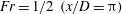
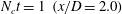
Figure 2. Three repeat internal wavefield measurements at
 $\mathit{Fr}=1/{\rm\pi}$
,
$\mathit{Fr}=1/{\rm\pi}$
,
 $Nt=2{\rm\pi}~(x/D=2.0)$
. The towed sphere is centred at
$Nt=2{\rm\pi}~(x/D=2.0)$
. The towed sphere is centred at
 $y=z=0$
. Dashed lines are probe locations. Wavefield displacements are to the same scale.
$y=z=0$
. Dashed lines are probe locations. Wavefield displacements are to the same scale.
3. Results
3.1. Description of IW data and scope of experiments
As mentioned, figure 2 shows three cross-track IW repeat runs. The towed sphere was centred at
 $y=0$
,
$y=0$
,
 $z=0$
, so that its vertical extent is
$z=0$
, so that its vertical extent is
 $D/2=4.25~\text{cm}$
. Near the sphere depth,
$D/2=4.25~\text{cm}$
. Near the sphere depth,
 $z=0$
to
$z=0$
to
 ${\sim}4~\text{cm}$
, the presence of the turbulent wake is evident. These data are aliased, as the data acquisition rate, sufficient to capture the IW field, was inadequate to capture the turbulent fluctuations (further studies on the wake density fluctuations have been performed and have been reported by Brandt & Schemm (Reference Brandt and Schemm2011)). Above this region, the vertical structure of the IW field is evident. (The wave amplitudes are plotted on the same scale as the vertical axis, showing the probe depth positions.) The lack of exact repeatability of the IW field is attributed to the random wave contributions and to some degree of experimental error. Differences between repeat runs are less pronounced with increasing height above the wake in accordance with the expectation that the random IWs would have shorter wavelengths and thus slower vertical propagation speeds than the lee waves, as discussed in Gilreath & Brandt (Reference Gilreath and Brandt1985). The residual differences between repeat runs outside the turbulent wake region are likely to be due to the contribution of the recirculating near-wake region behind the sphere, which is inherently not exactly repeatable, as well as minor differences in the ambient stratification between runs.
${\sim}4~\text{cm}$
, the presence of the turbulent wake is evident. These data are aliased, as the data acquisition rate, sufficient to capture the IW field, was inadequate to capture the turbulent fluctuations (further studies on the wake density fluctuations have been performed and have been reported by Brandt & Schemm (Reference Brandt and Schemm2011)). Above this region, the vertical structure of the IW field is evident. (The wave amplitudes are plotted on the same scale as the vertical axis, showing the probe depth positions.) The lack of exact repeatability of the IW field is attributed to the random wave contributions and to some degree of experimental error. Differences between repeat runs are less pronounced with increasing height above the wake in accordance with the expectation that the random IWs would have shorter wavelengths and thus slower vertical propagation speeds than the lee waves, as discussed in Gilreath & Brandt (Reference Gilreath and Brandt1985). The residual differences between repeat runs outside the turbulent wake region are likely to be due to the contribution of the recirculating near-wake region behind the sphere, which is inherently not exactly repeatable, as well as minor differences in the ambient stratification between runs.
An extensive series of experiments has been performed to explore the evolution of the IW field in the low-Froude-number early-wake regime. As discussed above, the stratification was maintained constant so that the values of
 $\mathit{Fr}$
and
$\mathit{Fr}$
and
 $\mathit{Re}$
were determined solely by the model speed. The scope of the run combinations exploring the effects of Froude number at
$\mathit{Re}$
were determined solely by the model speed. The scope of the run combinations exploring the effects of Froude number at
 $Nt=2{\rm\pi}$
is shown in table 1. The number of repeat runs,
$Nt=2{\rm\pi}$
is shown in table 1. The number of repeat runs,
 $n$
, at each condition is also shown. For a limited number of runs, a weaker stratification was used,
$n$
, at each condition is also shown. For a limited number of runs, a weaker stratification was used,
 $N=0.20~\text{s}^{-1}$
, as shown in the bottom rows in table 1. At
$N=0.20~\text{s}^{-1}$
, as shown in the bottom rows in table 1. At
 $N=0.20~\text{s}^{-1}$
, a value of
$N=0.20~\text{s}^{-1}$
, a value of
 $\mathit{Fr}=5$
was attained. Higher values of
$\mathit{Fr}=5$
was attained. Higher values of
 $\mathit{Fr}$
could not be attained, because, at higher speeds in the weak stratification, the turbulent wake was significantly larger, encompassing a large portion of the probe rake, thus invalidating the IW measurements. The individual runs were grouped in narrow bins representative of each value of
$\mathit{Fr}$
could not be attained, because, at higher speeds in the weak stratification, the turbulent wake was significantly larger, encompassing a large portion of the probe rake, thus invalidating the IW measurements. The individual runs were grouped in narrow bins representative of each value of
 $\mathit{Fr}$
. Shown in table 1 are the standard deviations of the run parameters for each run group; the low values justify the nominally identical conditions within each run group.
$\mathit{Fr}$
. Shown in table 1 are the standard deviations of the run parameters for each run group; the low values justify the nominally identical conditions within each run group.
Table 1. Run conditions for Froude-number variation experiments at
 $Nt=2{\rm\pi}~(N_{c}t=1.0)$
.
$Nt=2{\rm\pi}~(N_{c}t=1.0)$
.

While the present experimental effort was focused on examination of Froude-number variations, the effect of the corresponding Reynolds-number variations is of potential concern. The experiments were performed within a Reynolds-number regime where the unstratified drag on the sphere is essentially constant (Schlichting Reference Schlichting1968), so that the effects of the stratified background on the sphere drag can be clearly identified with Froude-number effects, as shown by Lofquist & Purtell (Reference Lofquist and Purtell1984) and Greenslade (Reference Greenslade2000). It can therefore be inferred that the nature of the internal wavefield is dominated by stratification, i.e. Froude-number variations rather than Reynolds-number effects. Moreover, at the one condition where
 $N$
was varied,
$N$
was varied,
 $\mathit{Fr}\approx 2$
, and the Reynolds numbers were
$\mathit{Fr}\approx 2$
, and the Reynolds numbers were
 $4.1\times 10^{3}$
and
$4.1\times 10^{3}$
and
 $22.0\times 10^{3}$
, the computed IW PE shown in figure 10 had essentially the same values, further implying the dominance of Froude-number effects on the nature of the IW field.
$22.0\times 10^{3}$
, the computed IW PE shown in figure 10 had essentially the same values, further implying the dominance of Froude-number effects on the nature of the IW field.
A series of runs was also made to explore the temporal (or downstream) evolution of the IW field. At each combination of
 $\mathit{Fr}$
and
$\mathit{Fr}$
and
 $Nt$
values, a number of runs were made (typically three to five for the
$Nt$
values, a number of runs were made (typically three to five for the
 $\mathit{Fr}$
variation study, and four to 10 for the
$\mathit{Fr}$
variation study, and four to 10 for the
 $Nt$
variation study) to ensure repeatability and to explore the contribution of the random IWs. Table 2 presents a listing of the runs exploring variations in
$Nt$
variation study) to ensure repeatability and to explore the contribution of the random IWs. Table 2 presents a listing of the runs exploring variations in
 $Nt$
at
$Nt$
at
 $\mathit{Fr}=1/{\rm\pi}\approx 0.32$
. The downstream locations were selected to have roughly equal spacing in terms of the number of BV cycles, i.e. nominal values of
$\mathit{Fr}=1/{\rm\pi}\approx 0.32$
. The downstream locations were selected to have roughly equal spacing in terms of the number of BV cycles, i.e. nominal values of
 $N_{c}t=\{1.0,1.5,2.0,2.5,3.0\}$
, where
$N_{c}t=\{1.0,1.5,2.0,2.5,3.0\}$
, where
 $N_{c}=N/2{\rm\pi}$
, with the time and downstream distance measured from the sphere centre. (Correspondingly the cyclic Froude number,
$N_{c}=N/2{\rm\pi}$
, with the time and downstream distance measured from the sphere centre. (Correspondingly the cyclic Froude number,
 $\mathit{Fr}_{c}=2{\rm\pi}\mathit{Fr}$
, for these runs was
$\mathit{Fr}_{c}=2{\rm\pi}\mathit{Fr}$
, for these runs was
 $\mathit{Fr}_{c}=2.0$
. For the Froude-number variation study,
$\mathit{Fr}_{c}=2.0$
. For the Froude-number variation study,
 $\mathit{Fr}_{c}=\{0.60,12.2\}$
.) For the range of test conditions,
$\mathit{Fr}_{c}=\{0.60,12.2\}$
.) For the range of test conditions,
 $\mathit{Re}=\{1.1,22.0\}\times 10^{3}$
. As the primary experimental variable was the towing speed of the sphere, the variations in
$\mathit{Re}=\{1.1,22.0\}\times 10^{3}$
. As the primary experimental variable was the towing speed of the sphere, the variations in
 $\mathit{Fr}$
were accompanied by changes in
$\mathit{Fr}$
were accompanied by changes in
 $\mathit{Re}$
. In the
$\mathit{Re}$
. In the
 $\mathit{Re}$
range employed,
$\mathit{Re}$
range employed,
 $\mathit{Re}$
is sufficiently large to be within the turbulent regime where the nominal, unstratified, drag coefficient is essentially constant (Schlichting Reference Schlichting1968), implying that, for the stratified flows considered herein, the generation of body-generated IWs is primarily a function of the Froude number, while the turbulent wake and the associated wake-generated IWs can be characterized in terms of both
$\mathit{Re}$
is sufficiently large to be within the turbulent regime where the nominal, unstratified, drag coefficient is essentially constant (Schlichting Reference Schlichting1968), implying that, for the stratified flows considered herein, the generation of body-generated IWs is primarily a function of the Froude number, while the turbulent wake and the associated wake-generated IWs can be characterized in terms of both
 $\mathit{Fr}$
and
$\mathit{Fr}$
and
 $\mathit{Re}$
.
$\mathit{Re}$
.

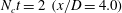
Figure 3. Four repeat internal wavefield measurements (thin lines) and their mean (thick line) at
 $\mathit{Fr}=1/{\rm\pi}$
,
$\mathit{Fr}=1/{\rm\pi}$
,
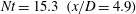 $Nt=15.3~(x/D=4.9)$
. The towed sphere is centred at
$Nt=15.3~(x/D=4.9)$
. The towed sphere is centred at
 $y=z=0$
and shown as a shaded region. Dashed lines are probe locations. Wavefield displacements are to the same scale.
$y=z=0$
and shown as a shaded region. Dashed lines are probe locations. Wavefield displacements are to the same scale.
Table 2. Run conditions for downstream variation experiments at
 $\mathit{Fr}=1/{\rm\pi}~(\mathit{Fr}_{c}=2.0)$
.
$\mathit{Fr}=1/{\rm\pi}~(\mathit{Fr}_{c}=2.0)$
.

3.2. Mean wavefield
3.2.1. Experimental results
Figure 3 presents four independent realizations and their mean of the cross-track IW fields at
 $\mathit{Fr}=1/{\rm\pi}$
,
$\mathit{Fr}=1/{\rm\pi}$
,
 $Nt=15.3$
. These data are at the same Froude number as the IWs shown in figure 2, but at a later time/downstream distance (
$Nt=15.3$
. These data are at the same Froude number as the IWs shown in figure 2, but at a later time/downstream distance (
 $x/D=FNt=4.9$
compared to
$x/D=FNt=4.9$
compared to
 $x/D=2.0$
in figure 2). In figure 3, the evolution of the wavefield at 2.5 cycles (
$x/D=2.0$
in figure 2). In figure 3, the evolution of the wavefield at 2.5 cycles (
 $N_{c}t=2.43$
) is manifested in terms of two waves on each side of the centreline resulting from the continuous forcing by the sphere and its attached recirculating region, as compared to the single symmetric wave evident in figure 2. The mean of the four wavefield realizations reduces the effects of the turbulent wake-generated IWs and the variability due to forcing by the near-wake recirculating region, and provides a characterization of the body forcing component of the IW field. The run-to-run variability of the IW field is the result of the unsteady recirculation zone behind the sphere and the random turbulent wake generated IWs. It also should be kept in mind that towed sphere IWs result from a translating source, significantly different from continuous forcing by, for example, a vertically oscillating cylinder (e.g. Mowbray & Rarity Reference Mowbray and Rarity1967). The mean IW fields for each group of runs, listed in tables 1 and 2, are used to characterize the
$N_{c}t=2.43$
) is manifested in terms of two waves on each side of the centreline resulting from the continuous forcing by the sphere and its attached recirculating region, as compared to the single symmetric wave evident in figure 2. The mean of the four wavefield realizations reduces the effects of the turbulent wake-generated IWs and the variability due to forcing by the near-wake recirculating region, and provides a characterization of the body forcing component of the IW field. The run-to-run variability of the IW field is the result of the unsteady recirculation zone behind the sphere and the random turbulent wake generated IWs. It also should be kept in mind that towed sphere IWs result from a translating source, significantly different from continuous forcing by, for example, a vertically oscillating cylinder (e.g. Mowbray & Rarity Reference Mowbray and Rarity1967). The mean IW fields for each group of runs, listed in tables 1 and 2, are used to characterize the
 $\mathit{Fr}$
and
$\mathit{Fr}$
and
 $Nt$
dependences.
$Nt$
dependences.

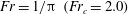
Figure 4. Froude-number dependence of mean internal wavefield,
 $Nt=2{\rm\pi}$
: (a)
$Nt=2{\rm\pi}$
: (a)
 $\mathit{Fr}=1/(2{\rm\pi})~(x/D=1.0)$
; (b)
$\mathit{Fr}=1/(2{\rm\pi})~(x/D=1.0)$
; (b)
 $\mathit{Fr}=1/2~(x/D={\rm\pi})$
; (c)
$\mathit{Fr}=1/2~(x/D={\rm\pi})$
; (c)
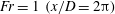 $\mathit{Fr}=1~(x/D=2{\rm\pi})$
; (d)
$\mathit{Fr}=1~(x/D=2{\rm\pi})$
; (d)
 $\mathit{Fr}=2~(x/D=4{\rm\pi})$
.
$\mathit{Fr}=2~(x/D=4{\rm\pi})$
.
3.2.2. Froude-number effects
The mean IW fields for four series of runs is shown in figure 4 in dimensionless coordinates scaled by the sphere radius,
 $R$
, illustrating the nature of the internal wavefield at different Froude numbers at one BV period,
$R$
, illustrating the nature of the internal wavefield at different Froude numbers at one BV period,
 $Nt=2{\rm\pi}$
. (It should be noted that, at a fixed value of
$Nt=2{\rm\pi}$
. (It should be noted that, at a fixed value of
 $x/D$
, rather than a fixed value of
$x/D$
, rather than a fixed value of
 $Nt$
, as shown in figure 4, the variation of the internal wavefield pattern would be dominated by the number of BV cycles elapsed as
$Nt$
, as shown in figure 4, the variation of the internal wavefield pattern would be dominated by the number of BV cycles elapsed as
 $Nt=(x/D)/\mathit{Fr}$
, much like the patterns shown in figure 5.) In these plots, IW forcing due to the body generation is evident by the uniformity of the wavefield at lower Froude numbers (figure 4
a,b) and at larger distances above the sphere wake. In contrast, wavefield distortions and asymmetries resulting from wake-generated IWs are present close to the sphere (
$Nt=(x/D)/\mathit{Fr}$
, much like the patterns shown in figure 5.) In these plots, IW forcing due to the body generation is evident by the uniformity of the wavefield at lower Froude numbers (figure 4
a,b) and at larger distances above the sphere wake. In contrast, wavefield distortions and asymmetries resulting from wake-generated IWs are present close to the sphere (
 $z/R\lesssim 1$
) and are considerably stronger at the higher-
$z/R\lesssim 1$
) and are considerably stronger at the higher-
 $\mathit{Fr}$
, higher-
$\mathit{Fr}$
, higher-
 $\mathit{Re}$
conditions (figure 4
c,d). The presence of random wake-generated IWs at these early times is in agreement with the calculations based on (1.2) discussed above; for example, at
$\mathit{Re}$
conditions (figure 4
c,d). The presence of random wake-generated IWs at these early times is in agreement with the calculations based on (1.2) discussed above; for example, at
 $\mathit{Fr}=2$
(figure 4
d), random IWs would be present at
$\mathit{Fr}=2$
(figure 4
d), random IWs would be present at
 $Nt\sim {\rm\pi}$
, well before the time of these IW measurements. The asymmetry in the internal wavefield evident at the higher
$Nt\sim {\rm\pi}$
, well before the time of these IW measurements. The asymmetry in the internal wavefield evident at the higher
 $\mathit{Fr}$
(and
$\mathit{Fr}$
(and
 $\mathit{Re}$
) values shown in figure 4(d) is due to the fact that, at these high values, the random wake turbulence is the dominant contributor to the internal wavefield. As a result, the number of ensemble runs averaged is not sufficient to provide an accurate mean wavefield. The integrated internal wavefield PE, however, has considerably less variability as discussed in § 3.4.2.
$\mathit{Re}$
) values shown in figure 4(d) is due to the fact that, at these high values, the random wake turbulence is the dominant contributor to the internal wavefield. As a result, the number of ensemble runs averaged is not sufficient to provide an accurate mean wavefield. The integrated internal wavefield PE, however, has considerably less variability as discussed in § 3.4.2.

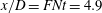
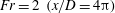
Figure 5. Temporal evolution of mean internal wavefield,
 $\mathit{Fr}=1/{\rm\pi}$
: (a)
$\mathit{Fr}=1/{\rm\pi}$
: (a)
 $N_{c}t=1~(x/D=2.0)$
; (b)
$N_{c}t=1~(x/D=2.0)$
; (b)
 $N_{c}t=2~(x/D=4.0)$
; (c)
$N_{c}t=2~(x/D=4.0)$
; (c)
 $N_{c}t=3~(x/D=6.0)$
.
$N_{c}t=3~(x/D=6.0)$
.
Qualitatively, the amplitudes of the IWs in the region above the turbulent wake
 $z/R\gtrsim 1$
appear to be larger at the intermediate Froude numbers (figure 4
b,c). This is indicative of a stronger coupling of the body source to the IW field at specific values of Froude number, as found in earlier studies, and will be further discussed in § 3.4. Since the limited ensemble used to estimate the mean internal wavefield as shown in figure 4 does entirely remove the random waves, the region of their influence is considered. The spread of wavefronts in the random IW field can be computed from the expressions given by Voisin (Reference Voisin1994) for a translating oscillating dipole at arbitrary values of
$z/R\gtrsim 1$
appear to be larger at the intermediate Froude numbers (figure 4
b,c). This is indicative of a stronger coupling of the body source to the IW field at specific values of Froude number, as found in earlier studies, and will be further discussed in § 3.4. Since the limited ensemble used to estimate the mean internal wavefield as shown in figure 4 does entirely remove the random waves, the region of their influence is considered. The spread of wavefronts in the random IW field can be computed from the expressions given by Voisin (Reference Voisin1994) for a translating oscillating dipole at arbitrary values of
 ${\it\Upsilon}$
in the parametric form
${\it\Upsilon}$
in the parametric form
 $$\begin{eqnarray}(y,z)=x\tan {\it\theta}_{\pm }\left(\frac{|\text{sin}{\it\phi}|}{{\it\Upsilon}}\right)(\cos ,\text{sin}){\it\phi},\end{eqnarray}$$
where
 ${\it\phi}$
is the azimuthal angle and
${\it\phi}$
is the azimuthal angle and
 ${\it\theta}_{\pm }(|\text{sin}{\it\phi}|/{\it\Upsilon})$
is the polar angle. For the present experiments, (1.2b
),
${\it\theta}_{\pm }(|\text{sin}{\it\phi}|/{\it\Upsilon})$
is the polar angle. For the present experiments, (1.2b
),
 ${\it\Upsilon}=\{0.1,6.3\}$
, it can be shown that, when the wavefield is decomposed into sum and difference components, the wavefronts become increasingly confined to a narrow band around the
${\it\Upsilon}=\{0.1,6.3\}$
, it can be shown that, when the wavefield is decomposed into sum and difference components, the wavefronts become increasingly confined to a narrow band around the
 $y=0$
axis (Voisin Reference Voisin1994). This agrees with the observed asymmetry in figure 4(d) that is confined to
$y=0$
axis (Voisin Reference Voisin1994). This agrees with the observed asymmetry in figure 4(d) that is confined to
 $y/R\lesssim \pm 3$
. The strength of the random IW field is dependent on the strength and scales of the coherent eddies in the turbulent wake, which are functions of
$y/R\lesssim \pm 3$
. The strength of the random IW field is dependent on the strength and scales of the coherent eddies in the turbulent wake, which are functions of
 $\mathit{Re}$
and
$\mathit{Re}$
and
 $\mathit{Fr}$
, and how they are related to the dipole source in this model.
$\mathit{Fr}$
, and how they are related to the dipole source in this model.
3.2.3. IW propagation in the vertical plane
The temporal evolution of the mean IW field at
 $\mathit{Fr}=0.32$
over three successive BV periods,
$\mathit{Fr}=0.32$
over three successive BV periods,
 $N_{c}t=\{1.0,2.0,3.0\}$
, is shown in figure 5. The effective body forcing due to the body itself and the near-field recirculating wake, the latter of which is not as effective as the body in displacing the surrounding fluid, generates the IW field with an increasing number of waves, corresponding roughly to the number of elapsed BV periods. In addition to the strong wavefield displacement directly above the sphere that was evident in the slender-body experiments in Gilreath & Brandt (Reference Gilreath and Brandt1985), the angle,
$N_{c}t=\{1.0,2.0,3.0\}$
, is shown in figure 5. The effective body forcing due to the body itself and the near-field recirculating wake, the latter of which is not as effective as the body in displacing the surrounding fluid, generates the IW field with an increasing number of waves, corresponding roughly to the number of elapsed BV periods. In addition to the strong wavefield displacement directly above the sphere that was evident in the slender-body experiments in Gilreath & Brandt (Reference Gilreath and Brandt1985), the angle,
 ${\it\theta}$
, of the IW beams with the vertical and the propagation of the IWs are evident in the present data. The wave beam angle is related to the effective forcing frequency,
${\it\theta}$
, of the IW beams with the vertical and the propagation of the IWs are evident in the present data. The wave beam angle is related to the effective forcing frequency,
 ${\it\omega}$
, by the linear dispersion relationship (Mowbray & Rarity Reference Mowbray and Rarity1967)
${\it\omega}$
, by the linear dispersion relationship (Mowbray & Rarity Reference Mowbray and Rarity1967)
 $$\begin{eqnarray}\frac{{\it\omega}}{N}=\cos {\it\theta},\end{eqnarray}$$
where
 ${\it\theta}$
is the angle between the wave group speed and the vertical. The present IW data are cross-track vertical plane cuts through the wave beams, so that a line through successive wave crests (and troughs) along the beam corresponds to the direction of the IW group velocity,
${\it\theta}$
is the angle between the wave group speed and the vertical. The present IW data are cross-track vertical plane cuts through the wave beams, so that a line through successive wave crests (and troughs) along the beam corresponds to the direction of the IW group velocity,
 $c_{g}$
. It is recognized that the actual structure of the wavefield is such that wave rays emanating from the sphere have varying frequency and inclinations, as illustrated in Voisin (Reference Voisin1994, Reference Voisin2007) and Vasholz (Reference Vasholz2011) and particularly in the combined mode plots in Sharman & Wurtele (Reference Sharman and Wurtele1983) and the cross-plane cuts illustrated in Sturova (Reference Sturova1978, Reference Sturova1980). Nevertheless, the experimental cross-plane cuts show an apparent dominant wave pattern, which is used to qualitatively characterize the wavefield, as has been employed in other experimental investigations (e.g. Cerasoli Reference Cerasoli1978; Dohan & Sutherland Reference Dohan and Sutherland2005). This wavefield characterization approach also pertains to the cuts in the horizontal plane discussed in § 3.2.4.
$c_{g}$
. It is recognized that the actual structure of the wavefield is such that wave rays emanating from the sphere have varying frequency and inclinations, as illustrated in Voisin (Reference Voisin1994, Reference Voisin2007) and Vasholz (Reference Vasholz2011) and particularly in the combined mode plots in Sharman & Wurtele (Reference Sharman and Wurtele1983) and the cross-plane cuts illustrated in Sturova (Reference Sturova1978, Reference Sturova1980). Nevertheless, the experimental cross-plane cuts show an apparent dominant wave pattern, which is used to qualitatively characterize the wavefield, as has been employed in other experimental investigations (e.g. Cerasoli Reference Cerasoli1978; Dohan & Sutherland Reference Dohan and Sutherland2005). This wavefield characterization approach also pertains to the cuts in the horizontal plane discussed in § 3.2.4.
To estimate
 ${\it\theta}$
, the angles of the crest and trough of the first wave (farthest off track) and the crest of the second wave were measured. These were readily tracked through the sequence of conditions listed in table 2, as illustrated by the dashed lines in figure 5. The evolution of the measured angles is shown in figure 6(a) in terms of
${\it\theta}$
, the angles of the crest and trough of the first wave (farthest off track) and the crest of the second wave were measured. These were readily tracked through the sequence of conditions listed in table 2, as illustrated by the dashed lines in figure 5. The evolution of the measured angles is shown in figure 6(a) in terms of
 ${\it\omega}/N$
according to (3.2), with an average
${\it\omega}/N$
according to (3.2), with an average
 ${\it\omega}/N\simeq 0.5$
,
${\it\omega}/N\simeq 0.5$
,
 ${\it\theta}\simeq 60^{\circ }$
and a spread corresponding to
${\it\theta}\simeq 60^{\circ }$
and a spread corresponding to
 ${\it\theta}\simeq 55^{\circ }{-}65^{\circ }$
. The estimated measurement error is
${\it\theta}\simeq 55^{\circ }{-}65^{\circ }$
. The estimated measurement error is
 ${\sim}10\,\%$
for these data, as well as for the wavelength values shown in figure 6(b). These values of
${\sim}10\,\%$
for these data, as well as for the wavelength values shown in figure 6(b). These values of
 ${\it\theta}$
are somewhat larger than the range measured by Dohan & Sutherland (Reference Dohan and Sutherland2005),
${\it\theta}$
are somewhat larger than the range measured by Dohan & Sutherland (Reference Dohan and Sutherland2005),
 ${\it\theta}=46\pm 5^{\circ }$
, for IWs generated by a continuous turbulent source, by Cerasoli (Reference Cerasoli1978) for IWs resulting from the collapse of a buoyant plume where the angle ranged between
${\it\theta}=46\pm 5^{\circ }$
, for IWs generated by a continuous turbulent source, by Cerasoli (Reference Cerasoli1978) for IWs resulting from the collapse of a buoyant plume where the angle ranged between
 ${\it\theta}=35^{\circ }$
and
${\it\theta}=35^{\circ }$
and
 $50^{\circ }$
, and by Wu (Reference Wu1969) for the collapse of a mixed region where
$50^{\circ }$
, and by Wu (Reference Wu1969) for the collapse of a mixed region where
 ${\it\theta}=36^{\circ }$
. In numerical simulations of wake turbulence, steeper angles were found by Diamessis & Abdilghanie (Reference Diamessis and Abdilghanie2011), with
${\it\theta}=36^{\circ }$
. In numerical simulations of wake turbulence, steeper angles were found by Diamessis & Abdilghanie (Reference Diamessis and Abdilghanie2011), with
 ${\it\theta}=31^{\circ }$
at low
${\it\theta}=31^{\circ }$
at low
 $\mathit{Re}=5\times 10^{3}$
and
$\mathit{Re}=5\times 10^{3}$
and
 ${\it\theta}=45^{\circ }$
at the higher
${\it\theta}=45^{\circ }$
at the higher
 $\mathit{Re}=10^{5}$
. These lower angles are not unreasonable since the turbulent wake-generated IWs have shorter wavelengths and higher frequencies than the body displacement IWs. Dohan & Sutherland (Reference Dohan and Sutherland2005) have used linear theory to estimate the angle at which the waves carry the maximum vertical flux away from a turbulent source as
$\mathit{Re}=10^{5}$
. These lower angles are not unreasonable since the turbulent wake-generated IWs have shorter wavelengths and higher frequencies than the body displacement IWs. Dohan & Sutherland (Reference Dohan and Sutherland2005) have used linear theory to estimate the angle at which the waves carry the maximum vertical flux away from a turbulent source as
 $45^{\circ }~({\it\omega}/N=0.7)$
. Deviations of the experimental data from this value could be due to experimental error and/or nonlinear interaction effects.
$45^{\circ }~({\it\omega}/N=0.7)$
. Deviations of the experimental data from this value could be due to experimental error and/or nonlinear interaction effects.

Figure 6. Internal wave propagation in the vertical plane,
 $\mathit{Fr}=1/{\rm\pi}$
. (a) Effective forcing frequency (wave angle according to dispersion relation, (3.2)): ●, first crest; ▪, first trough; ♦, second crest. (b) Horizontal wavelength: ●,
$\mathit{Fr}=1/{\rm\pi}$
. (a) Effective forcing frequency (wave angle according to dispersion relation, (3.2)): ●, first crest; ▪, first trough; ♦, second crest. (b) Horizontal wavelength: ●,
 $z/R=2.11$
; ▪,
$z/R=2.11$
; ▪,
 $z/R=2.11$
; ♦,
$z/R=2.11$
; ♦,
 $z/R=3.79$
.
$z/R=3.79$
.
Wavelengths associated with the mean IW field were estimated from the temporal evolution data represented by figure 5. Figure 6(b) shows the IW wavelengths,
 ${\it\lambda}$
, measured at three elevations above the turbulent region where the body-generated IWs clearly dominate, using peak-to-trough values of the clearly dominant wave. While these data are limited, the increase in
${\it\lambda}$
, measured at three elevations above the turbulent region where the body-generated IWs clearly dominate, using peak-to-trough values of the clearly dominant wave. While these data are limited, the increase in
 ${\it\lambda}/D$
with distance from the source and with increasing values of
${\it\lambda}/D$
with distance from the source and with increasing values of
 $Nt$
is apparent. (Chomaz et al. (Reference Chomaz, Bonneton and Hopfinger1993b
) found that the horizontal along-track wavelength (as opposed to the cross-track measurements obtained herein) was strongly
$Nt$
is apparent. (Chomaz et al. (Reference Chomaz, Bonneton and Hopfinger1993b
) found that the horizontal along-track wavelength (as opposed to the cross-track measurements obtained herein) was strongly
 $\mathit{Fr}$
-dependent, with a value of
$\mathit{Fr}$
-dependent, with a value of
 ${\it\lambda}/D\simeq 8$
at
${\it\lambda}/D\simeq 8$
at
 $\mathit{Fr}=0.32$
.) The present values of
$\mathit{Fr}=0.32$
.) The present values of
 ${\it\lambda}/D$
are considerably greater than the wavelengths computed by Diamessis & Abdilghanie (Reference Diamessis and Abdilghanie2011) and Abdilghanie & Diamessis (Reference Abdilghanie and Diamessis2013) for turbulent wake-generated IWs of
${\it\lambda}/D$
are considerably greater than the wavelengths computed by Diamessis & Abdilghanie (Reference Diamessis and Abdilghanie2011) and Abdilghanie & Diamessis (Reference Abdilghanie and Diamessis2013) for turbulent wake-generated IWs of
 ${\it\lambda}/D\simeq 1.5$
for
${\it\lambda}/D\simeq 1.5$
for
 $\mathit{Fr}=2$
in the range of
$\mathit{Fr}=2$
in the range of
 $N_{c}t=1.6{-}30$
. This is expected since the lee wave forcing scale is considerably larger than the characteristic dimension of the wake eddies.
$N_{c}t=1.6{-}30$
. This is expected since the lee wave forcing scale is considerably larger than the characteristic dimension of the wake eddies.
The increase in the spreading angle and increased wavelengths further from the source were explained by Cerasoli (Reference Cerasoli1978) based on an argument of Wu (Reference Wu1969). In effect, as the IWs are generated by a broadband source, the waves with longer wavelengths will have larger phase and group speeds than those with shorter wavelengths, with the result that they will propagate farther from the source and more rapidly propagate off track, resulting in an increasing angle of the rays connecting the crests and troughs.
3.2.4. IW spreading in the horizontal plane
Horizontal (
 $x{-}y$
plane) spreading of the IW field was investigated by plotting the mean IW amplitudes at specified depths for the seven
$x{-}y$
plane) spreading of the IW field was investigated by plotting the mean IW amplitudes at specified depths for the seven
 $Nt$
conditions at
$Nt$
conditions at
 $\mathit{Fr}=1/{\rm\pi}$
given in table 2. The resulting plots at three depths are shown in figure 7. Connecting the crests and troughs of the evolving waveforms, as illustrated by the dashed lines in figure 7, illustrates the spreading, or local ‘opening angle’,
$\mathit{Fr}=1/{\rm\pi}$
given in table 2. The resulting plots at three depths are shown in figure 7. Connecting the crests and troughs of the evolving waveforms, as illustrated by the dashed lines in figure 7, illustrates the spreading, or local ‘opening angle’,
 ${\it\phi}$
, of the IW pattern with time (or downstream distance). Measured values of
${\it\phi}$
, of the IW pattern with time (or downstream distance). Measured values of
 ${\it\phi}$
for the off-centre wave troughs and crests are shown in figure 8. (The value at
${\it\phi}$
for the off-centre wave troughs and crests are shown in figure 8. (The value at
 $z/D=1.9$
was computed as a least-squares fit to the off-track distance of each of the individual IW wave crests (40 total) listed in table 2, as a check.) Clearly
$z/D=1.9$
was computed as a least-squares fit to the off-track distance of each of the individual IW wave crests (40 total) listed in table 2, as a check.) Clearly
 ${\it\phi}$
increases with height above the sphere; this is in accordance with the low-
${\it\phi}$
increases with height above the sphere; this is in accordance with the low-
 $\mathit{Fr}$
analytical model (Vasholz Reference Vasholz2011). Here,
$\mathit{Fr}$
analytical model (Vasholz Reference Vasholz2011). Here,
 ${\it\phi}$
increases in an approximately linear manner with distance above the sphere, with outermost trough spreading faster, in agreement with the increased wave speed associated with the longer wavelengths at larger distances from the sphere (discussed in § 3.2.3).
${\it\phi}$
increases in an approximately linear manner with distance above the sphere, with outermost trough spreading faster, in agreement with the increased wave speed associated with the longer wavelengths at larger distances from the sphere (discussed in § 3.2.3).

Figure 7. Internal wavefield spreading,
 $\mathit{Fr}=1/{\rm\pi}$
: (a)
$\mathit{Fr}=1/{\rm\pi}$
: (a)
 $z/R=1.05$
; (b)
$z/R=1.05$
; (b)
 $z/R=2.11$
; (c)
$z/R=2.11$
; (c)
 $z/R=3.16$
.
$z/R=3.16$
.

Figure 8. Internal wavefield opening angle,
 $\mathit{Fr}=1/{\rm\pi}$
: ●, first trough; ▪, first crest.
$\mathit{Fr}=1/{\rm\pi}$
: ●, first trough; ▪, first crest.
The opening angles computed by Robey (Reference Robey1997) for the mode-1 IWs and by the equation derived by Vasholz (Reference Vasholz2011) for the lower modes (i.e. modes 1, 2 and 3) are considerably narrower than observed in the present experiments. This difference can be attributed to the fact that, in contrast to the later-time evolution modelled by Robey (Reference Robey1997) and Vasholz (Reference Vasholz2011), where the opening angles were computed for IW evolution over 15 cycles (
 $N_{c}t\leqslant 15$
), the present results are confined to the very near field (i.e. three cycles,
$N_{c}t\leqslant 15$
), the present results are confined to the very near field (i.e. three cycles,
 $N_{c}t\leqslant 3$
) where the broadband IW source is generating a signature that is, from the analytic perspective, the sum of multiple modes that often do not have a clear pattern, as demonstrated by Sharman & Wurtele (Reference Sharman and Wurtele1983). However, the experimental results shown by Robey (Reference Robey1997) show a significantly wider band of IWs at early times at low
$N_{c}t\leqslant 3$
) where the broadband IW source is generating a signature that is, from the analytic perspective, the sum of multiple modes that often do not have a clear pattern, as demonstrated by Sharman & Wurtele (Reference Sharman and Wurtele1983). However, the experimental results shown by Robey (Reference Robey1997) show a significantly wider band of IWs at early times at low
 $\mathit{Fr}$
, extending beyond the central band, which matches the mode-1 calculations. Geometrically scaling
$\mathit{Fr}$
, extending beyond the central band, which matches the mode-1 calculations. Geometrically scaling
 ${\it\phi}$
for the broader waves at the lowest speed shown by Robey (Reference Robey1997), which corresponds to
${\it\phi}$
for the broader waves at the lowest speed shown by Robey (Reference Robey1997), which corresponds to
 $\mathit{Fr}=0.44$
, yields
$\mathit{Fr}=0.44$
, yields
 ${\it\phi}\approx 32^{\circ }$
. This is in agreement with the present results (figure 8) considering that Robey’s measurements are for a pycnocline stratification, in contrast to the uniform stratification of the present experiments.
${\it\phi}\approx 32^{\circ }$
. This is in agreement with the present results (figure 8) considering that Robey’s measurements are for a pycnocline stratification, in contrast to the uniform stratification of the present experiments.
3.3. Turbulent wake
While measurement of the properties of the turbulent wake itself was not the primary objective of the present study, it was possible to use the cross-plane displacement data to determine the wake geometric properties. In general, the turbulent wake contains both wave-like and turbulent-like motions, which are difficult, if not impossible, to clearly separate (Jacobitz, Rogers & Ferziger Reference Jacobitz, Rogers and Ferziger2005; Brandt & Schemm Reference Brandt and Schemm2011; Vasil’ev, Voropaeva & Kurbatskii Reference Vasil’ev, Voropaeva and Kurbatskii2011). As the data in the wake region are aliased as a result of insufficient sampling in the turbulent region, as evident in figure 2, only a determination of the boundaries of the region containing the high-frequency fluctuations could be obtained, providing estimates of the height and width of the turbulent wake region. In general, it can be observed from the present data (e.g. figures 2 and 3) that the turbulent wake region extends to a height of
 $z/D\approx 0.45$
, in agreement with the calculations of Abdilghanie & Diamessis (Reference Abdilghanie and Diamessis2013), where the wake extends to
$z/D\approx 0.45$
, in agreement with the calculations of Abdilghanie & Diamessis (Reference Abdilghanie and Diamessis2013), where the wake extends to
 $z/D=0.5$
at comparable
$z/D=0.5$
at comparable
 $\mathit{Fr}$
and
$\mathit{Fr}$
and
 $\mathit{Re}$
.
$\mathit{Re}$
.
By trying several methods to delineate the wake, it was found that using a threshold level of the slope of cross-track IW PE density at each probe yielded a reasonably definitive demarcation of the wake region. The IW PE was computed using the square of the IW amplitude,
 ${\it\zeta}$
, at each point along the probe traverse as
${\it\zeta}$
, at each point along the probe traverse as
 $$\begin{eqnarray}\text{PE}={\textstyle \frac{1}{2}}{\it\rho}N^{2}{\it\zeta}^{2}.\end{eqnarray}$$
The evolution of the maximum wake height,
 $H_{w}$
, and width,
$H_{w}$
, and width,
 $W_{w}$
, determined for each run ensemble using this criterion is shown in figure 9 for the wake evolution data at
$W_{w}$
, determined for each run ensemble using this criterion is shown in figure 9 for the wake evolution data at
 $\mathit{Fr}=1/{\rm\pi}$
. The error bars represent the standard deviation for the runs in the each ensemble group; for the wake height, the maximum of the standard deviation and the probe spacing interval was used. Although these data encompass a limited down-track range,
$\mathit{Fr}=1/{\rm\pi}$
. The error bars represent the standard deviation for the runs in the each ensemble group; for the wake height, the maximum of the standard deviation and the probe spacing interval was used. Although these data encompass a limited down-track range,
 $x/D=2.0{-}6.1$
, the overall trends of wake height showing the collapse, due to the onset of buoyancy effects, and subsequent rise and the generally steady growth in wake width are in general agreement with prior results at higher Froude numbers (see e.g. Lin et al. (Reference Lin, Boyer and Fernando1992a
) for a towed sphere and Lin & Pao (Reference Lin and Pao1979) and Gilreath & Brandt (Reference Gilreath and Brandt1985) for self-propelled slender bodies).
$x/D=2.0{-}6.1$
, the overall trends of wake height showing the collapse, due to the onset of buoyancy effects, and subsequent rise and the generally steady growth in wake width are in general agreement with prior results at higher Froude numbers (see e.g. Lin et al. (Reference Lin, Boyer and Fernando1992a
) for a towed sphere and Lin & Pao (Reference Lin and Pao1979) and Gilreath & Brandt (Reference Gilreath and Brandt1985) for self-propelled slender bodies).

Figure 9. Evolution of turbulent wake,
 $\mathit{Fr}=1/{\rm\pi}$
: (a) wake height; (b) wake width (dashed line is
$\mathit{Fr}=1/{\rm\pi}$
: (a) wake height; (b) wake width (dashed line is
 $\propto (Nt)^{1/3}$
).
$\propto (Nt)^{1/3}$
).
Specifically, as shown in figure 9(a), the maximum wake height prior to collapse is
 $H_{w}/D=1.1$
and the extent of collapse is
$H_{w}/D=1.1$
and the extent of collapse is
 ${\rm\Delta}H_{w}/D=0.27$
. The wake geometry data at low
${\rm\Delta}H_{w}/D=0.27$
. The wake geometry data at low
 $\mathit{Fr}$
in Lin et al. (Reference Lin, Boyer and Fernando1992a
) show that, within the scatter of the data, the downstream location of the height minimum decreases as the Froude number decreases, with the minimum occurring at
$\mathit{Fr}$
in Lin et al. (Reference Lin, Boyer and Fernando1992a
) show that, within the scatter of the data, the downstream location of the height minimum decreases as the Froude number decreases, with the minimum occurring at
 $Nt=1.6$
at
$Nt=1.6$
at
 $\mathit{Fr}=1$
, with
$\mathit{Fr}=1$
, with
 $H_{w}/D\simeq 1.0$
and
$H_{w}/D\simeq 1.0$
and
 ${\rm\Delta}H_{w}/D\simeq 0.5$
. Comparisons to the present data are not unreasonable considering that the present data are at a considerably lower Froude number. Overall, however, the generally slow growth in
${\rm\Delta}H_{w}/D\simeq 0.5$
. Comparisons to the present data are not unreasonable considering that the present data are at a considerably lower Froude number. Overall, however, the generally slow growth in
 $H_{w}/D$
is in agreement with the essentially constant wake height in the
$H_{w}/D$
is in agreement with the essentially constant wake height in the
 $Nt<80$
regime described in the self-similar wake evolution diagram in Spedding (Reference Spedding2014, figure 3(b)).
$Nt<80$
regime described in the self-similar wake evolution diagram in Spedding (Reference Spedding2014, figure 3(b)).
The wake width (figure 9
b) grows as
 ${\sim}(Nt)^{1/3}$
in agreement with Lin et al. (Reference Lin, Boyer and Fernando1992a
) and Spedding et al. (Reference Spedding, Browand and Fincham1996b
), as shown by the dashed curve that is positioned to have
${\sim}(Nt)^{1/3}$
in agreement with Lin et al. (Reference Lin, Boyer and Fernando1992a
) and Spedding et al. (Reference Spedding, Browand and Fincham1996b
), as shown by the dashed curve that is positioned to have
 $W_{w}/D=1.0$
at
$W_{w}/D=1.0$
at
 $x/D=1.0~(Nt=3.1)$
. The levelling off of the present data at larger values of
$x/D=1.0~(Nt=3.1)$
. The levelling off of the present data at larger values of
 $Nt$
may be indicative of the decay of the turbulence within the wake at later times.
$Nt$
may be indicative of the decay of the turbulence within the wake at later times.
3.4. Internal wave potential energy
3.4.1. Variation of IW PE with Froude number
To characterize the strength of the IW field generated by the towed sphere, the PE per unit down-track distance within the probe rake aperture,
 $\text{PE}_{A}$
, was computed for each of the individual runs listed in tables 1 and 2.
$\text{PE}_{A}$
, was computed for each of the individual runs listed in tables 1 and 2.
 $\text{PE}_{A}$
was computed from the square of the wave amplitude,
$\text{PE}_{A}$
was computed from the square of the wave amplitude,
 ${\it\zeta}$
, along the probe rake cuts, integrated over rake aperture as
${\it\zeta}$
, along the probe rake cuts, integrated over rake aperture as
 $$\begin{eqnarray}\text{PE}_{A}=\iint _{(z,y)}\frac{1}{2}{\it\rho}_{0}N^{2}{\it\zeta}^{2}\,\text{d}y\,\text{d}z.\end{eqnarray}$$
Integration in the cross-track direction was carried out by summation of the displacements at each digitized point obtained as the probe rake traversed the IW field (0.6 cm apart). Vertical integration was performed by assuming that the IW field obtained for each probe is representative of the pattern halfway to the neighbouring probe. As the lower probes (those at
 $z/D<5$
) traversing the turbulent wake region are not measuring a clearly defined IW field (due to the presence of the turbulent wake discussed in § 3.2), and are aliased due to the sampling rate, the lowest five probes were excluded from the calculation of
$z/D<5$
) traversing the turbulent wake region are not measuring a clearly defined IW field (due to the presence of the turbulent wake discussed in § 3.2), and are aliased due to the sampling rate, the lowest five probes were excluded from the calculation of
 $\text{PE}_{A}$
; i.e. (3.4) is integrated over the range
$\text{PE}_{A}$
; i.e. (3.4) is integrated over the range
 $z/D=0.47{-}1.95$
. As the probe rake spanned 86 % of the stratified upper region of the water column,
$z/D=0.47{-}1.95$
. As the probe rake spanned 86 % of the stratified upper region of the water column,
 $\text{PE}_{A}$
provides a reasonable relative measure of the energy coupled into the IW field (extrapolation to the total PE is discussed in § 3.4.2).
$\text{PE}_{A}$
provides a reasonable relative measure of the energy coupled into the IW field (extrapolation to the total PE is discussed in § 3.4.2).
 $\text{PE}_{A}$
as a function of
$\text{PE}_{A}$
as a function of
 $\mathit{Fr}$
computed for each of the individual runs within each group listed in table 1 is shown in figure 10. While the IW traces at low
$\mathit{Fr}$
computed for each of the individual runs within each group listed in table 1 is shown in figure 10. While the IW traces at low
 $\mathit{Fr}$
appear qualitatively repeatable (see figures 2 and 3), the variability in
$\mathit{Fr}$
appear qualitatively repeatable (see figures 2 and 3), the variability in
 $\text{PE}_{A}$
is apparent. This is the result of variability of the forcing by the recirculation zone behind the sphere, and to some degree experimental error. At higher
$\text{PE}_{A}$
is apparent. This is the result of variability of the forcing by the recirculation zone behind the sphere, and to some degree experimental error. At higher
 $\mathit{Fr}$
,
$\mathit{Fr}$
,
 $\mathit{Fr}\geqslant 1$
, the spread in
$\mathit{Fr}\geqslant 1$
, the spread in
 $\text{PE}_{A}$
reflects the inherent variability due to the contributions from the turbulent wake. As discussed in § 2.1, most of the data were obtained with a linear stratification of
$\text{PE}_{A}$
reflects the inherent variability due to the contributions from the turbulent wake. As discussed in § 2.1, most of the data were obtained with a linear stratification of
 $N=1.20~\text{s}^{-1}$
. To achieve higher values of
$N=1.20~\text{s}^{-1}$
. To achieve higher values of
 $\mathit{Fr}$
, the stratification was reduced to
$\mathit{Fr}$
, the stratification was reduced to
 $N=0.20~\text{s}^{-1}$
, shown by the unfilled points in figure 10 at
$N=0.20~\text{s}^{-1}$
, shown by the unfilled points in figure 10 at
 $\mathit{Fr}\approx 2$
and 5. The general agreement of the
$\mathit{Fr}\approx 2$
and 5. The general agreement of the
 $\text{PE}_{A}$
values at
$\text{PE}_{A}$
values at
 $\mathit{Fr}\approx 2$
for both stratifications provides a level of confirmation of the overall approach. Data obtained at a higher tow speed in the weak stratification to achieve
$\mathit{Fr}\approx 2$
for both stratifications provides a level of confirmation of the overall approach. Data obtained at a higher tow speed in the weak stratification to achieve
 $\mathit{Fr}\approx 10$
had substantially larger wake turbulence displacements extending well beyond the designated wake region,
$\mathit{Fr}\approx 10$
had substantially larger wake turbulence displacements extending well beyond the designated wake region,
 $z/D\leqslant 0.45$
, prohibiting the use of these data for computing
$z/D\leqslant 0.45$
, prohibiting the use of these data for computing
 $\text{PE}_{A}$
.
$\text{PE}_{A}$
.

Figure 10. Froude-number dependence of IW PE,
 $Nt=2{\rm\pi}$
: ●,
$Nt=2{\rm\pi}$
: ●,
 $N=1.20~\text{s}^{-1}$
; ▫,
$N=1.20~\text{s}^{-1}$
; ▫,
 $N=0.20~\text{s}^{-1}$
. Long dashed line is
$N=0.20~\text{s}^{-1}$
. Long dashed line is
 $\propto \mathit{Fr}^{2}$
; short dashed line is (3.6),
$\propto \mathit{Fr}^{2}$
; short dashed line is (3.6),
 $\propto \mathit{Fr}^{7/2}$
.
$\propto \mathit{Fr}^{7/2}$
.
Figure 10 illustrates the existence of several regimes characterizing the coupling between the body-generated lee waves at low
 $\mathit{Fr}$
and the turbulent wake-generated IWs at larger
$\mathit{Fr}$
and the turbulent wake-generated IWs at larger
 $\mathit{Fr}$
. In the lee wave regime at low
$\mathit{Fr}$
. In the lee wave regime at low
 $\mathit{Fr}$
,
$\mathit{Fr}$
,
 $\mathit{Fr}\leqslant 0.5$
,
$\mathit{Fr}\leqslant 0.5$
,
 $\text{PE}_{A}$
increases approximately
$\text{PE}_{A}$
increases approximately
 $\propto \mathit{Fr}^{2}$
, reaches a maximum at
$\propto \mathit{Fr}^{2}$
, reaches a maximum at
 $\mathit{Fr}\sim 0.5$
, and decreases until
$\mathit{Fr}\sim 0.5$
, and decreases until
 $\mathit{Fr}\approx 1$
. At this point the turbulent wake becomes the dominant source of IWs and
$\mathit{Fr}\approx 1$
. At this point the turbulent wake becomes the dominant source of IWs and
 $\text{PE}_{A}$
again increases. These trends resulting from the present comprehensive measurements of the sphere-generated IW field are in general agreement with prior more limited observations that generally considered only the amplitude of a specific constant density level. The observed low-
$\text{PE}_{A}$
again increases. These trends resulting from the present comprehensive measurements of the sphere-generated IW field are in general agreement with prior more limited observations that generally considered only the amplitude of a specific constant density level. The observed low-
 $\mathit{Fr}$
growth rate of
$\mathit{Fr}$
growth rate of
 $\text{PE}_{A}\propto \mathit{Fr}^{2}$
agrees with the wave amplitude growth rate
$\text{PE}_{A}\propto \mathit{Fr}^{2}$
agrees with the wave amplitude growth rate
 $\propto \mathit{Fr}$
observed by Chomaz et al. (Reference Chomaz, Bonneton and Hopfinger1993b
) (note that the PE is proportional to the square of the wave amplitude as seen in (3.4)). This result differs, however, from the amplitude growth rate
$\propto \mathit{Fr}$
observed by Chomaz et al. (Reference Chomaz, Bonneton and Hopfinger1993b
) (note that the PE is proportional to the square of the wave amplitude as seen in (3.4)). This result differs, however, from the amplitude growth rate
 $\propto \mathit{Fr}^{2}$
found by Robey (Reference Robey1997), which is most certainly the result of the pycnocline stratification that trapped the internal wavefield. It should be noted, however, that lee wave displacements produced in different vertical regions are predicted to have different Froude-number dependences (Greenslade Reference Greenslade2000; Voisin Reference Voisin2007), so that the comparisons of the present data that are an integrated average over the entire wavefield to the wave amplitudes measured at specific locations by Chomaz et al. (Reference Chomaz, Bonneton and Hopfinger1993b
) and Robey (Reference Robey1997) should be considered as qualitative. The Froude number at which the resonant lee wave coupling maximum occurs agrees with observations of Chomaz et al. (Reference Chomaz, Bonneton and Hopfinger1993b
) and Robey (Reference Robey1997) and with the peak in the sphere drag measured by Lofquist & Purtell (Reference Lofquist and Purtell1984), and it is reasonably close to the analytical prediction of
$\propto \mathit{Fr}^{2}$
found by Robey (Reference Robey1997), which is most certainly the result of the pycnocline stratification that trapped the internal wavefield. It should be noted, however, that lee wave displacements produced in different vertical regions are predicted to have different Froude-number dependences (Greenslade Reference Greenslade2000; Voisin Reference Voisin2007), so that the comparisons of the present data that are an integrated average over the entire wavefield to the wave amplitudes measured at specific locations by Chomaz et al. (Reference Chomaz, Bonneton and Hopfinger1993b
) and Robey (Reference Robey1997) should be considered as qualitative. The Froude number at which the resonant lee wave coupling maximum occurs agrees with observations of Chomaz et al. (Reference Chomaz, Bonneton and Hopfinger1993b
) and Robey (Reference Robey1997) and with the peak in the sphere drag measured by Lofquist & Purtell (Reference Lofquist and Purtell1984), and it is reasonably close to the analytical prediction of
 $\mathit{Fr}\sim 0.46$
(Vasholz Reference Vasholz2002). Further comparisons to lee wave models are presented in § 3.4.3. Finally, the transition between the lee wave and the turbulent wake generation regimes agrees with the
$\mathit{Fr}\sim 0.46$
(Vasholz Reference Vasholz2002). Further comparisons to lee wave models are presented in § 3.4.3. Finally, the transition between the lee wave and the turbulent wake generation regimes agrees with the
 $\mathit{Fr}\approx 2$
location noted by Chomaz et al. (Reference Chomaz, Bonneton, Butet, Hopfinger, Perrier, Metais and Lesieur1991), Hopfinger et al. (Reference Hopfinger, Flor, Chomaz and Bonneton1991), Lin et al. (Reference Lin, Boyer and Fernando1993) and Robey (Reference Robey1997). The large run-to-run variation in
$\mathit{Fr}\approx 2$
location noted by Chomaz et al. (Reference Chomaz, Bonneton, Butet, Hopfinger, Perrier, Metais and Lesieur1991), Hopfinger et al. (Reference Hopfinger, Flor, Chomaz and Bonneton1991), Lin et al. (Reference Lin, Boyer and Fernando1993) and Robey (Reference Robey1997). The large run-to-run variation in
 $\text{PE}_{A}$
at
$\text{PE}_{A}$
at
 $\mathit{Fr}=2$
and 5 (and to some degree at
$\mathit{Fr}=2$
and 5 (and to some degree at
 $\mathit{Fr}=1$
) is due to the presence of wake turbulence-generated IWs, as further discussed in the following section.
$\mathit{Fr}=1$
) is due to the presence of wake turbulence-generated IWs, as further discussed in the following section.
3.4.2. Total PE in the IW field
Using the measurements of
 $\text{PE}_{A}$
, it is possible to estimate the fraction of the total input energy that is manifest in the internal wavefield. To obtain this estimate, it is assumed that the region of the water column covered by the probes (86 % of the upper half) is representative of the whole water column, so that increasing
$\text{PE}_{A}$
, it is possible to estimate the fraction of the total input energy that is manifest in the internal wavefield. To obtain this estimate, it is assumed that the region of the water column covered by the probes (86 % of the upper half) is representative of the whole water column, so that increasing
 $\text{PE}_{A}$
by a factor of 1.16 and multiplying by 2 (to account for the bottom half of the IW field) will yield the total IW PE,
$\text{PE}_{A}$
by a factor of 1.16 and multiplying by 2 (to account for the bottom half of the IW field) will yield the total IW PE,
 $\text{PE}_{T}$
, exclusive of that present within the turbulent wake region. Because of these approximations, estimates of the total IW PE should be considered somewhat more qualitative than quantitative.
$\text{PE}_{T}$
, exclusive of that present within the turbulent wake region. Because of these approximations, estimates of the total IW PE should be considered somewhat more qualitative than quantitative.
For a towed body, the total energy input per unit down-track distance to the turbulent wake and the internal wavefield is equal to the drag force on the sphere,
 $\mathscr{D}=({\it\rho}C_{D}U^{2}A)/2$
, where
$\mathscr{D}=({\it\rho}C_{D}U^{2}A)/2$
, where
 $C_{D}$
is the drag coefficient and
$C_{D}$
is the drag coefficient and
 $A$
is the sphere cross-sectional area. For spheres in a stratified flow, detailed measurements of
$A$
is the sphere cross-sectional area. For spheres in a stratified flow, detailed measurements of
 $\mathscr{D}$
in terms of changes in
$\mathscr{D}$
in terms of changes in
 $C_{D}$
as a function of
$C_{D}$
as a function of
 $\mathit{Fr}$
were made by Lofquist & Purtell (Reference Lofquist and Purtell1984). It should also be noted that the Reynolds-number regime considered is lower than that where the drag crisis exists (
$\mathit{Fr}$
were made by Lofquist & Purtell (Reference Lofquist and Purtell1984). It should also be noted that the Reynolds-number regime considered is lower than that where the drag crisis exists (
 $\mathit{Re}<5\times 10^{4}$
for roughened spheres), so that sphere roughness does not affect its drag due to the fact that the boundary layer separates while it is still laminar with the roughness elements embedded within the boundary layer (Hoerner Reference Hoerner1958; Achenbach Reference Achenbach1974). These values are used to compute
$\mathit{Re}<5\times 10^{4}$
for roughened spheres), so that sphere roughness does not affect its drag due to the fact that the boundary layer separates while it is still laminar with the roughness elements embedded within the boundary layer (Hoerner Reference Hoerner1958; Achenbach Reference Achenbach1974). These values are used to compute
 $\mathscr{D}$
in figure 11(a), which shows the ratio of
$\mathscr{D}$
in figure 11(a), which shows the ratio of
 $\text{PE}_{T}$
to the measured sphere drag as a function of
$\text{PE}_{T}$
to the measured sphere drag as a function of
 $\mathit{Fr}$
. These values were obtained by averaging the values of
$\mathit{Fr}$
. These values were obtained by averaging the values of
 $\text{PE}_{A}$
computed from each of the individual runs at each condition listed in table 1, grouped into local
$\text{PE}_{A}$
computed from each of the individual runs at each condition listed in table 1, grouped into local
 $\mathit{Fr}$
bins in order to provide a more accurate estimate. The error bars show the standard error of the mean for each bin. Here,
$\mathit{Fr}$
bins in order to provide a more accurate estimate. The error bars show the standard error of the mean for each bin. Here,
 $\text{PE}_{T}$
represents an estimate of the total IW PE resulting from both the body and turbulent wake sources.
$\text{PE}_{T}$
represents an estimate of the total IW PE resulting from both the body and turbulent wake sources.

Figure 11. Total wavefield PE,
 $Nt=2{\rm\pi}$
. (a) PE as fraction of energy input: ▪,
$Nt=2{\rm\pi}$
. (a) PE as fraction of energy input: ▪,
 $\text{PE}_{T}$
; ●,
$\text{PE}_{T}$
; ●,
 $\text{PE}_{TA}$
. Short dashed line is
$\text{PE}_{TA}$
. Short dashed line is
 $\propto \mathit{Fr}^{1/2}$
; long dashed line is
$\propto \mathit{Fr}^{1/2}$
; long dashed line is
 $\propto \mathit{Fr}^{-2}$
, dotted line is (3.8). (b) Random wake forcing contribution to total PE.
$\propto \mathit{Fr}^{-2}$
, dotted line is (3.8). (b) Random wake forcing contribution to total PE.
The most striking result shown is the strong coupling of the input energy to the IW field in the regime
 $0.2\lesssim \mathit{Fr}\lesssim 0.6$
, where
$0.2\lesssim \mathit{Fr}\lesssim 0.6$
, where
 $\text{PE}_{T}/\mathscr{D}$
ranges from 40 % to 70 %. The balance of the total energy input is manifest as the kinetic energy (KE) associated with the IWs and the PE and KE in the turbulent wake. This strong coupling results from the balance between the larger IW PE at higher
$\text{PE}_{T}/\mathscr{D}$
ranges from 40 % to 70 %. The balance of the total energy input is manifest as the kinetic energy (KE) associated with the IWs and the PE and KE in the turbulent wake. This strong coupling results from the balance between the larger IW PE at higher
 $\mathit{Fr}$
(figure 10) and the increased drag at lower
$\mathit{Fr}$
(figure 10) and the increased drag at lower
 $\mathit{Fr}$
(Lofquist & Purtell Reference Lofquist and Purtell1984) and can be explained in terms of the inherent environmental resonance of the stratified flow field (Vasholz Reference Vasholz2002). In this low-
$\mathit{Fr}$
(Lofquist & Purtell Reference Lofquist and Purtell1984) and can be explained in terms of the inherent environmental resonance of the stratified flow field (Vasholz Reference Vasholz2002). In this low-
 $\mathit{Fr}$
regime, where
$\mathit{Fr}$
regime, where
 $\text{PE}_{A}$
increases considerably (
$\text{PE}_{A}$
increases considerably (
 $\propto \mathit{Fr}^{2}$
) towards the resonance peak, the fraction of the total input energy,
$\propto \mathit{Fr}^{2}$
) towards the resonance peak, the fraction of the total input energy,
 $\text{PE}_{T}/\mathscr{D}$
, going into the IW field, increasing at only a moderate rate, is approximately
$\text{PE}_{T}/\mathscr{D}$
, going into the IW field, increasing at only a moderate rate, is approximately
 $\propto \mathit{Fr}^{1/2}$
, as shown by the short dashed line in figure 11(a).
$\propto \mathit{Fr}^{1/2}$
, as shown by the short dashed line in figure 11(a).
For values of
 $\mathit{Fr}\gtrsim 1$
, where the turbulent wake source becomes dominant,
$\mathit{Fr}\gtrsim 1$
, where the turbulent wake source becomes dominant,
 $\text{PE}_{T}/\mathscr{D}$
decreases with
$\text{PE}_{T}/\mathscr{D}$
decreases with
 $\mathit{Fr}$
by almost two orders of magnitude by
$\mathit{Fr}$
by almost two orders of magnitude by
 $\mathit{Fr}\sim 5$
, despite the fact that the turbulent wake-generated IW contribution increases with
$\mathit{Fr}\sim 5$
, despite the fact that the turbulent wake-generated IW contribution increases with
 $\mathit{Fr}$
when
$\mathit{Fr}$
when
 $\mathit{Fr}\gtrsim 1$
(figure 10), indicating a larger fraction of energy going into wake turbulence itself. This is qualitatively in agreement with the numerical simulations of turbulent wake-generated IW of Abdilghanie & Diamessis (Reference Abdilghanie and Diamessis2013), which show a decrease in wake momentum lost, presumably to the IW field, as
$\mathit{Fr}\gtrsim 1$
(figure 10), indicating a larger fraction of energy going into wake turbulence itself. This is qualitatively in agreement with the numerical simulations of turbulent wake-generated IW of Abdilghanie & Diamessis (Reference Abdilghanie and Diamessis2013), which show a decrease in wake momentum lost, presumably to the IW field, as
 $\mathit{Fr}$
increases using simulations at
$\mathit{Fr}$
increases using simulations at
 $\mathit{Fr}=2$
, 8 and 32.
$\mathit{Fr}=2$
, 8 and 32.
Alternatively, computing PE from the mean of the measured wavefield amplitudes at each test condition, designated
 $\text{PE}_{TA}$
, results in a measure of the repeatable component of the IW field, as shown in figure 11(a). In the strong coupling region,
$\text{PE}_{TA}$
, results in a measure of the repeatable component of the IW field, as shown in figure 11(a). In the strong coupling region,
 $0.2\lesssim \mathit{Fr}\lesssim 0.6$
, the non-repeatable component of the
$0.2\lesssim \mathit{Fr}\lesssim 0.6$
, the non-repeatable component of the
 $\text{PE}_{T}$
is small: the difference,
$\text{PE}_{T}$
is small: the difference,
 $(\text{PE}_{T}-\text{PE}_{TA})/\text{PE}_{T}$
, is shown in figure 11(b). The increase in
$(\text{PE}_{T}-\text{PE}_{TA})/\text{PE}_{T}$
, is shown in figure 11(b). The increase in
 $(\text{PE}_{T}-\text{PE}_{TA})/\text{PE}_{T}$
at low values of
$(\text{PE}_{T}-\text{PE}_{TA})/\text{PE}_{T}$
at low values of
 $\mathit{Fr}$
is probably the result of variations in
$\mathit{Fr}$
is probably the result of variations in
 $\text{PE}_{T}$
due to the fact that at these low
$\text{PE}_{T}$
due to the fact that at these low
 $\mathit{Fr}$
values the
$\mathit{Fr}$
values the
 $\text{PE}_{T}/\mathscr{D}$
and
$\text{PE}_{T}/\mathscr{D}$
and
 $\text{PE}_{TA}/\mathscr{D}$
are ratios of two small numbers (cf. figure 10). While the integrated PE estimates shown in figures 11 and 12 do not show any direct evidence of depth-dependent resonances at discrete values of
$\text{PE}_{TA}/\mathscr{D}$
are ratios of two small numbers (cf. figure 10). While the integrated PE estimates shown in figures 11 and 12 do not show any direct evidence of depth-dependent resonances at discrete values of
 $\mathit{Fr}_{H}$
(as discussed in § 1.3), the finite tank depth would be a contributing factor to the observed IW PE levels. In the large-
$\mathit{Fr}_{H}$
(as discussed in § 1.3), the finite tank depth would be a contributing factor to the observed IW PE levels. In the large-
 $\mathit{Fr}$
region,
$\mathit{Fr}$
region,
 $\mathit{Fr}\gtrsim 1$
,
$\mathit{Fr}\gtrsim 1$
,
 $\text{PE}_{TA}/\mathscr{D}$
decreases
$\text{PE}_{TA}/\mathscr{D}$
decreases
 $\propto \mathit{Fr}^{-2}$
(shown as the long dashed line), indicative of the lessening influence of the lee wave forcing mechanism, while
$\propto \mathit{Fr}^{-2}$
(shown as the long dashed line), indicative of the lessening influence of the lee wave forcing mechanism, while
 $\text{PE}_{T}/\mathscr{D}$
decreases at a slower rate, approximately
$\text{PE}_{T}/\mathscr{D}$
decreases at a slower rate, approximately
 $\propto \mathit{Fr}^{-3/2}$
, indicating the increased IW forcing by the turbulent wake, the fraction of which is shown in figure 11(b).
$\propto \mathit{Fr}^{-3/2}$
, indicating the increased IW forcing by the turbulent wake, the fraction of which is shown in figure 11(b).

Figure 12. Temporal evolution of wavefield total PE,
 $\mathit{Fr}=1/{\rm\pi}$
. (a) PE as fraction of energy input: ▪,
$\mathit{Fr}=1/{\rm\pi}$
. (a) PE as fraction of energy input: ▪,
 $\text{PE}_{T}$
; ●,
$\text{PE}_{T}$
; ●,
 $\text{PE}_{TA}$
. (b) Random wake forcing contribution to total PE.
$\text{PE}_{TA}$
. (b) Random wake forcing contribution to total PE.
3.4.3. Comparisons to lee wave models
Bell (Reference Bell1975) developed a two-dimensional linear solution for lee waves generated by a topographic (body) source in an oscillating flow. For a particular topographic shape, a solution for the dimensionless power,
 $\overline{\mathscr{P}}/({\rm\pi}/4){\it\rho}_{0}U_{0}^{2}ND^{2}$
(rate of energy), being fed to the internal wavefield at zero oscillation frequency (steady flow) in the low-
$\overline{\mathscr{P}}/({\rm\pi}/4){\it\rho}_{0}U_{0}^{2}ND^{2}$
(rate of energy), being fed to the internal wavefield at zero oscillation frequency (steady flow) in the low-
 $\mathit{Fr}$
limit (
$\mathit{Fr}$
limit (
 $\mathit{Fr}\rightarrow 0$
) is a constant. When converted from power to energy per unit distance using the average over one BV cycle and then to the dimensionless form used herein results in energy/
$\mathit{Fr}\rightarrow 0$
) is a constant. When converted from power to energy per unit distance using the average over one BV cycle and then to the dimensionless form used herein results in energy/
 $({\it\rho}N^{2}D^{4})\sim ({\rm\pi}^{2}/4)\mathit{Fr}^{2}$
, which agrees with the experimentally determined behaviour at low
$({\it\rho}N^{2}D^{4})\sim ({\rm\pi}^{2}/4)\mathit{Fr}^{2}$
, which agrees with the experimentally determined behaviour at low
 $\mathit{Fr}$
shown in figure 10. The actual values, however, are more than an order of magnitude larger than the present experimental values of IW PE. Owing to the differences between Bell’s model and the present experiment (i.e. Bell (Reference Bell1975) considers a two-dimensional continuous reinforcing flow over a specific mountain shape (witch of Agnesi) as compared to the present transient forcing situation), only qualitative agreement would be expected. Thus the agreement of Bell’s result with the apparent trend in figure 10 is somewhat fortuitous.
$\mathit{Fr}$
shown in figure 10. The actual values, however, are more than an order of magnitude larger than the present experimental values of IW PE. Owing to the differences between Bell’s model and the present experiment (i.e. Bell (Reference Bell1975) considers a two-dimensional continuous reinforcing flow over a specific mountain shape (witch of Agnesi) as compared to the present transient forcing situation), only qualitative agreement would be expected. Thus the agreement of Bell’s result with the apparent trend in figure 10 is somewhat fortuitous.
As the pressure drag on the sphere results from the generation of IWs and the separation of the boundary layer from the sphere surface, modelling of the sphere drag has been divided into two components. Semi-empirical relationships for the Froude number dependence of lee wave drag have been derived by Greenslade (Reference Greenslade2000), Voisin (Reference Voisin2007) and Dalziel et al. (Reference Dalziel, Patterson, Caulfied and Le Brun2011) for both the wave and wake contributions. For the low-
 $\mathit{Fr}$
limit,
$\mathit{Fr}$
limit,
 $\mathit{Fr}\rightarrow 0$
, the corresponding drag coefficients are
$\mathit{Fr}\rightarrow 0$
, the corresponding drag coefficients are
 $C_{D}^{wave}\propto \mathit{Fr}^{3/2}$
and
$C_{D}^{wave}\propto \mathit{Fr}^{3/2}$
and
 $C_{D}^{wake}\propto \mathit{Fr}^{1/2}$
. For comparison to the present IW PE results, consider the wave component given by
$C_{D}^{wake}\propto \mathit{Fr}^{1/2}$
. For comparison to the present IW PE results, consider the wave component given by
 $$\begin{eqnarray}C_{D}^{wave}=2^{3/2}B\mathit{Fr}^{3/2},\end{eqnarray}$$
where
 $B$
is based on the empirical fit to the experimental data or the analytically derived value of
$B$
is based on the empirical fit to the experimental data or the analytically derived value of
 $B=(32\sqrt{2})/15{\rm\pi}\simeq 0.960$
(Voisin Reference Voisin2007) and the Froude number based on the sphere radius is converted to the present diameter-based Froude number. Thus the drag due to the induced waves
$B=(32\sqrt{2})/15{\rm\pi}\simeq 0.960$
(Voisin Reference Voisin2007) and the Froude number based on the sphere radius is converted to the present diameter-based Froude number. Thus the drag due to the induced waves
 $\mathscr{D}^{wave}=({\it\rho}C_{D}^{wave}U^{2}({\rm\pi}D^{2}/4))/2$
, converted to the present scaling, is given by
$\mathscr{D}^{wave}=({\it\rho}C_{D}^{wave}U^{2}({\rm\pi}D^{2}/4))/2$
, converted to the present scaling, is given by
 $$\begin{eqnarray}\frac{\mathscr{D}^{wave}}{{\it\rho}N^{2}D^{4}}=1.22\frac{{\rm\pi}}{8}B\mathit{Fr}^{7/2},\end{eqnarray}$$
where the factor 1.22 results from the finite aperture of the probe rake as discussed in § 3.4.2.
As
 $\mathscr{D}^{wave}$
is equivalent to the energy per unit downstream input into the IW field by lee wave forcing, this relation is shown on figure 10 as a short dashed line. The slope of this theoretical estimate matches reasonably well with the experimental data for
$\mathscr{D}^{wave}$
is equivalent to the energy per unit downstream input into the IW field by lee wave forcing, this relation is shown on figure 10 as a short dashed line. The slope of this theoretical estimate matches reasonably well with the experimental data for
 $\mathit{Fr}\lesssim 0.3$
; however, the magnitude given by (3.5) is slightly low. A value of the constant
$\mathit{Fr}\lesssim 0.3$
; however, the magnitude given by (3.5) is slightly low. A value of the constant
 $B\approx 2.5$
would fit the data. This difference could be the result of effects of the finite depth of the tank.
$B\approx 2.5$
would fit the data. This difference could be the result of effects of the finite depth of the tank.
The total IW PE at low
 $\mathit{Fr}$
shown in figure 11 can be compared to (3.5) by computing the wave component of the lee wave drag as a fraction of the total lee wave drag as
$\mathit{Fr}$
shown in figure 11 can be compared to (3.5) by computing the wave component of the lee wave drag as a fraction of the total lee wave drag as
 $\mathscr{D}^{wave}/\mathscr{D}=C_{D}^{wave}/(C_{D}^{wave}+C_{D}^{wake})$
, with
$\mathscr{D}^{wave}/\mathscr{D}=C_{D}^{wave}/(C_{D}^{wave}+C_{D}^{wake})$
, with
 $$\begin{eqnarray}C_{D}^{wake}=2^{1/2}C\mathit{Fr}^{1/2}(1+{\textstyle \frac{5}{2}}\mathit{Fr}),\end{eqnarray}$$
where
 $C$
is a fit to the experimental drag measurement data (Voisin Reference Voisin2007), yielding
$C$
is a fit to the experimental drag measurement data (Voisin Reference Voisin2007), yielding
 $$\begin{eqnarray}\frac{\mathscr{D}^{wave}}{\mathscr{D}}=\left[\frac{1}{2}\frac{C}{B}\mathit{Fr}^{-1}+\left(1-\frac{5}{4}\frac{C}{B}\right)\right]^{-1},\end{eqnarray}$$
approximately
 $\propto \mathit{Fr}$
. Using the analytic value for
$\propto \mathit{Fr}$
. Using the analytic value for
 $B$
and the drag data fitted value of
$B$
and the drag data fitted value of
 $C\approx 3.33$
(Voisin Reference Voisin2007), (3.8) is shown as a dotted line on figure 11, where it should be compared to
$C\approx 3.33$
(Voisin Reference Voisin2007), (3.8) is shown as a dotted line on figure 11, where it should be compared to
 $\text{PE}_{TA}/\mathscr{D}$
, as it represents the steady lee wave component. The agreement is quite reasonable.
$\text{PE}_{TA}/\mathscr{D}$
, as it represents the steady lee wave component. The agreement is quite reasonable.
Model comparison at high Froude numbers is rather problematical, as the lee wave models are inviscid and thus in the high-
 $\mathit{Fr}$
limit do not account for the turbulence-generated IWs, which tend to dominate at
$\mathit{Fr}$
limit do not account for the turbulence-generated IWs, which tend to dominate at
 $\mathit{Fr}\gtrsim 0.5$
. In the limit as
$\mathit{Fr}\gtrsim 0.5$
. In the limit as
 $\mathit{Fr}\rightarrow \infty$
,
$\mathit{Fr}\rightarrow \infty$
,
 $C_{D}^{wave}\propto \mathit{Fr}^{-4}$
and
$C_{D}^{wave}\propto \mathit{Fr}^{-4}$
and
 $C_{D}^{wake}\propto C_{D}(\infty )$
, where
$C_{D}^{wake}\propto C_{D}(\infty )$
, where
 $C_{D}(\infty )$
is the drag coefficient for the unstratified limit (Gorodtsov & Teodorovich Reference Gorodtsov and Teodorovich1982), taken as 0.51 based on the experimental studies (Voisin Reference Voisin2007). This results in
$C_{D}(\infty )$
is the drag coefficient for the unstratified limit (Gorodtsov & Teodorovich Reference Gorodtsov and Teodorovich1982), taken as 0.51 based on the experimental studies (Voisin Reference Voisin2007). This results in
 $\mathscr{D}^{wave}/({\it\rho}N^{2}D^{4})\propto \mathit{Fr}^{-2}$
and
$\mathscr{D}^{wave}/({\it\rho}N^{2}D^{4})\propto \mathit{Fr}^{-2}$
and
 $\mathscr{D}^{wave}/\mathscr{D}\propto \mathit{Fr}^{-4}$
, which as expected have a significantly greater falloff than the experimental data (figures 10 and 11) due to the additional presence of IWs resulting from the random wake eddies in the experimental data.
$\mathscr{D}^{wave}/\mathscr{D}\propto \mathit{Fr}^{-4}$
, which as expected have a significantly greater falloff than the experimental data (figures 10 and 11) due to the additional presence of IWs resulting from the random wake eddies in the experimental data.
3.4.4. Temporal evolution of total IW PE
It should be noted that these PE data, figures 10 and 11, represent the near-wake regime, at one BV period (
 $N_{c}t=1$
), so that the physical fluid displacement generating the IWs is still occurring (as also evident in the early-time evolution of the IW shown in Gilreath & Brandt (Reference Gilreath and Brandt1985)), causing a large contribution to the IW PE and less to the IW KE as the wavefield has not had time to equilibrate. Figure 12(a) shows the temporal evolution of both the
$N_{c}t=1$
), so that the physical fluid displacement generating the IWs is still occurring (as also evident in the early-time evolution of the IW shown in Gilreath & Brandt (Reference Gilreath and Brandt1985)), causing a large contribution to the IW PE and less to the IW KE as the wavefield has not had time to equilibrate. Figure 12(a) shows the temporal evolution of both the
 $\text{PE}_{T}$
and the repeatable component
$\text{PE}_{T}$
and the repeatable component
 $\text{PE}_{TA}$
as functions of downstream evolution for three BV periods for the test series listed in table 2. Each point shown represents the mean of the repeated runs at each value of
$\text{PE}_{TA}$
as functions of downstream evolution for three BV periods for the test series listed in table 2. Each point shown represents the mean of the repeated runs at each value of
 $N_{c}t$
, with the error bars representing the standard error of the mean for each value of
$N_{c}t$
, with the error bars representing the standard error of the mean for each value of
 $N_{c}t$
measured. The
$N_{c}t$
measured. The
 ${\sim}2/3$
decrease in
${\sim}2/3$
decrease in
 $\text{PE}_{TA}/\mathscr{D}$
with
$\text{PE}_{TA}/\mathscr{D}$
with
 $N_{c}t$
at
$N_{c}t$
at
 $N_{c}t=3.03$
from its maximum at
$N_{c}t=3.03$
from its maximum at
 $N_{c}t=1.45$
is indicative of the lessening influence of the lee wave generation mechanism and the trend towards IW equipartition. The increase in the non-repeatable component due to the increasing contribution of the turbulent wake IW source is evidenced by the decrease in
$N_{c}t=1.45$
is indicative of the lessening influence of the lee wave generation mechanism and the trend towards IW equipartition. The increase in the non-repeatable component due to the increasing contribution of the turbulent wake IW source is evidenced by the decrease in
 $\text{PE}_{T}/\mathscr{D}$
(by
$\text{PE}_{T}/\mathscr{D}$
(by
 ${\sim}1/3$
at
${\sim}1/3$
at
 $N_{c}t=3.03$
from its maximum at
$N_{c}t=3.03$
from its maximum at
 $N_{c}t=1.45$
) and the increased difference in
$N_{c}t=1.45$
) and the increased difference in
 $(\text{PE}_{T}-\text{PE}_{TA})/\text{PE}_{T}$
, shown in figure 12(b).
$(\text{PE}_{T}-\text{PE}_{TA})/\text{PE}_{T}$
, shown in figure 12(b).
4. Summary and discussion
An extensive experimental investigation of the near-field internal wavefield generated by a towed sphere at low Froude number in a uniformly stratified fluid has been performed. The results have provided a characterization of the wavefield patterns. Vertical spreading angles in the near field of
 ${\it\theta}\simeq 55^{\circ }{-}65^{\circ }$
were measured, which are considerably shallower than the angles characteristic of higher-
${\it\theta}\simeq 55^{\circ }{-}65^{\circ }$
were measured, which are considerably shallower than the angles characteristic of higher-
 $\mathit{Fr}$
turbulent IW sources. This is due to the inherently lower frequencies associated with the low-
$\mathit{Fr}$
turbulent IW sources. This is due to the inherently lower frequencies associated with the low-
 $\mathit{Fr}$
body generation mechanism. Wavefield spreading in the horizontal was found to increase with distance above the sphere, ranging over
$\mathit{Fr}$
body generation mechanism. Wavefield spreading in the horizontal was found to increase with distance above the sphere, ranging over
 ${\it\phi}=20^{\circ }{-}35^{\circ }$
for
${\it\phi}=20^{\circ }{-}35^{\circ }$
for
 $z/D=0.5{-}1.9$
. The increase in
$z/D=0.5{-}1.9$
. The increase in
 ${\it\phi}$
with distance is in agreement with the low-
${\it\phi}$
with distance is in agreement with the low-
 $\mathit{Fr}$
analytical model of Vasholz (Reference Vasholz2011). However, these values differ considerably from the far-field patterns evident in the experiments of Robey (Reference Robey1997) and point-source far-field models (e.g. Keller & Munk Reference Keller and Munk1970). This difference is due to the presence of significant contributions from higher IW modes in the near field. The early-time low-
$\mathit{Fr}$
analytical model of Vasholz (Reference Vasholz2011). However, these values differ considerably from the far-field patterns evident in the experiments of Robey (Reference Robey1997) and point-source far-field models (e.g. Keller & Munk Reference Keller and Munk1970). This difference is due to the presence of significant contributions from higher IW modes in the near field. The early-time low-
 $\mathit{Fr}$
experimental results shown by Robey (Reference Robey1997) show a significantly wider IW band that extends beyond the central band, which matches his mode-1 calculations and those of Vasholz (Reference Vasholz2011).
$\mathit{Fr}$
experimental results shown by Robey (Reference Robey1997) show a significantly wider IW band that extends beyond the central band, which matches his mode-1 calculations and those of Vasholz (Reference Vasholz2011).
Quantitative measurements of the IW PE, as a function of Froude number and distance behind the body, as well as the relative contributions of the IW generated by body forcing, rather than those generated by the turbulent wake, have been determined, extending the previous measurements of Gilreath & Brandt (Reference Gilreath and Brandt1985) and Robey (Reference Robey1997). Specifically, it was found that, at one BV period, the IW PE reached a maximum at
 $\mathit{Fr}\sim 0.5$
(figure 10), in agreement with the peak IW amplitude at
$\mathit{Fr}\sim 0.5$
(figure 10), in agreement with the peak IW amplitude at
 $\mathit{Fr}=0.5{-}0.7$
measured from particle streak images by Chomaz et al. (Reference Chomaz, Bonneton and Hopfinger1993b
) and in reasonable agreement with the peak amplitude at
$\mathit{Fr}=0.5{-}0.7$
measured from particle streak images by Chomaz et al. (Reference Chomaz, Bonneton and Hopfinger1993b
) and in reasonable agreement with the peak amplitude at
 $\mathit{Fr}=0.7{-}0.8$
measured from an individual probe in a pycnocline layer (Robey Reference Robey1997). It was found that up to 70 % of the input energy is converted to IWs at low
$\mathit{Fr}=0.7{-}0.8$
measured from an individual probe in a pycnocline layer (Robey Reference Robey1997). It was found that up to 70 % of the input energy is converted to IWs at low
 $\mathit{Fr}$
(figure 11). This peak in IW PE occurs in the regime
$\mathit{Fr}$
(figure 11). This peak in IW PE occurs in the regime
 $0.2\lesssim \mathit{Fr}\lesssim 0.6$
, corresponding to analytical prediction of a lee wave coupling resonance at
$0.2\lesssim \mathit{Fr}\lesssim 0.6$
, corresponding to analytical prediction of a lee wave coupling resonance at
 $\mathit{Fr}\sim 0.46$
(Vasholz Reference Vasholz2002) and explaining the increase in drag at low
$\mathit{Fr}\sim 0.46$
(Vasholz Reference Vasholz2002) and explaining the increase in drag at low
 $\mathit{Fr}$
observed by Lofquist & Purtell (Reference Lofquist and Purtell1984). At this early time, the effect of the body (lee wave) forcing is to displace the fluid, resulting in an imbalance in the PE/KE ratio that ameliorates as time progresses (figure 12). Although the IW KE was not measured, it is not unreasonable to conclude that, in this low-
$\mathit{Fr}$
observed by Lofquist & Purtell (Reference Lofquist and Purtell1984). At this early time, the effect of the body (lee wave) forcing is to displace the fluid, resulting in an imbalance in the PE/KE ratio that ameliorates as time progresses (figure 12). Although the IW KE was not measured, it is not unreasonable to conclude that, in this low-
 $\mathit{Fr}$
regime, virtually all of the input energy is manifest as IWs. At larger values,
$\mathit{Fr}$
regime, virtually all of the input energy is manifest as IWs. At larger values,
 $\mathit{Fr}\gtrsim 1$
, when the turbulent wake source contribution becomes significant, the energy input to the IW field increases considerably; however, the IW energy becomes a decreasing fraction of the input energy, the balance increasingly going into the turbulent wake.
$\mathit{Fr}\gtrsim 1$
, when the turbulent wake source contribution becomes significant, the energy input to the IW field increases considerably; however, the IW energy becomes a decreasing fraction of the input energy, the balance increasingly going into the turbulent wake.
Finally, it should be noted that at high
 $\mathit{Fr}$
(i.e.
$\mathit{Fr}$
(i.e.
 $\mathit{Fr}\gtrsim 1$
), where turbulent wake forcing becomes dominant, the IW field above the wake region has a coherent structure, as illustrated in figure 4(c,d) (albeit with asymmetries present at higher
$\mathit{Fr}\gtrsim 1$
), where turbulent wake forcing becomes dominant, the IW field above the wake region has a coherent structure, as illustrated in figure 4(c,d) (albeit with asymmetries present at higher
 $\mathit{Fr}$
due to the insufficient number of ensemble samples), similar to that present at lower-
$\mathit{Fr}$
due to the insufficient number of ensemble samples), similar to that present at lower-
 $\mathit{Fr}$
conditions (as shown in figures 2, 3 and 4
a,b). This is also observed in the case of a self-propelled slender body at
$\mathit{Fr}$
conditions (as shown in figures 2, 3 and 4
a,b). This is also observed in the case of a self-propelled slender body at
 $\mathit{Fr}=5.3$
as shown in Gilreath & Brandt (Reference Gilreath and Brandt1985), and for IW generated by a continuous turbulent source as in Dohan & Sutherland (Reference Dohan and Sutherland2005).
$\mathit{Fr}=5.3$
as shown in Gilreath & Brandt (Reference Gilreath and Brandt1985), and for IW generated by a continuous turbulent source as in Dohan & Sutherland (Reference Dohan and Sutherland2005).
Acknowledgements
The support of J. E. Hopkins in the conduct of the experiments, the effort of K. R. Shipley for review and editing, and the scientific collaboration with C. E. Schemm and H. E. Gilreath are greatly appreciated. This effort was supported by the Office of Naval Research Turbulence and Stratified Wakes Program, L. P. Purtell and R. D. Joslin, programme managers; their ongoing support is highly appreciated. The insightful comments of the anonymous reviewers resulted in significant improvements to the manuscript.


