


1 Introduction
The propagation of a hydrodynamic shock wave across an heterogeneous medium is a very important topic in many fields of application, e.g. aerospace engineering, nuclear engineering but also astrophysics. Such an interaction is known to emit a complex field, which is a mixture of acoustic, entropy and vortical waves according to Kovásznay’s decomposition (see Kovasznay Reference Kovasznay1953; Chu & Kovásznay Reference Chu and Kovásznay1958; Sagaut & Cambon Reference Sagaut and Cambon2018). In the limit of small disturbances, the emitted field can be accurately predicted considering a linearized theory, namely the linear interaction approximation (LIA), see Sagaut & Cambon (Reference Sagaut and Cambon2018) for an exhaustive discussion. This approximation is relevant in the wrinkled shock regime, in which the shock front corrugation by upstream disturbances is small enough to leave its topology unchanged, so that it can be decomposed as a linear sum of sinusoidal contributions. Several semi-empirical criteria of validity of LIA have been proposed on the grounds of direct numerical simulation (DNS) results. In the case of a turbulent upstream flow, Lee, Lele & Moin (Reference Lee, Lele and Moin1993) proposed
 $$\begin{eqnarray}M_{t}^{2}<0.1(M_{1}^{2}-1),\end{eqnarray}$$
where
 $M_{t}$
and
$M_{t}$
and
 $M_{1}$
are the upstream turbulent and mean Mach numbers, respectively. This criterion was later refined using DNS with higher resolution by Ryu & Livescu (Reference Ryu and Livescu2014), yielding
$M_{1}$
are the upstream turbulent and mean Mach numbers, respectively. This criterion was later refined using DNS with higher resolution by Ryu & Livescu (Reference Ryu and Livescu2014), yielding
 $$\begin{eqnarray}M_{t_{2}}\leqslant 0.1M_{2},\end{eqnarray}$$
with
 $M_{t_{2}}$
and
$M_{t_{2}}$
and
 $M_{2}$
the downstream (LIA-predicted) turbulent Mach number and the downstream mean flow-based Mach number, respectively. In the laminar case of the interaction between an entropy spot and a normal shock, Fabre, Jacquin & Sesterhenn (Reference Fabre, Jacquin and Sesterhenn2001) reported an excellent agreement within 1 % error up to
$M_{2}$
the downstream (LIA-predicted) turbulent Mach number and the downstream mean flow-based Mach number, respectively. In the laminar case of the interaction between an entropy spot and a normal shock, Fabre, Jacquin & Sesterhenn (Reference Fabre, Jacquin and Sesterhenn2001) reported an excellent agreement within 1 % error up to
 $M_{1}=4$
for disturbances with relative amplitude less than or equal to
$M_{1}=4$
for disturbances with relative amplitude less than or equal to
 $0.01$
.
$0.01$
.
This theory was pioneered in the 1950s by Moore (Reference Moore1953), Ribner (Reference Ribner1954a ,Reference Ribner b , Reference Ribner1959) and is still under development. The most complete formulation of the normal-mode analysis for canonical interaction was given by Fabre et al. (Reference Fabre, Jacquin and Sesterhenn2001), which was further extended to the case of the non-reacting binary mixture of perfect gases (Griffond Reference Griffond2005; Griffond, Soulard & Souffland Reference Griffond, Soulard and Souffland2010) and to rarefaction waves (Griffond & Soulard Reference Griffond and Soulard2012). Following this approach, wave vectors of emitted waves are obtained analytically thanks to the dispersion relation stemming from the linearized Euler equations, while wave amplitudes are solution of a linear system. A deeper physical insight is obtained by grouping upstream disturbances according to the Kovásznay normal-mode decomposition of small compressible fluctuations into acoustic, vorticity and entropy modes. This decomposition has been extended by splitting the vorticity mode into the sum of a poloidal and a toroidal component (Griffond & Soulard Reference Griffond and Soulard2012), and also considering a binary mixture of perfect gases (Griffond Reference Griffond2005, Reference Griffond2006). Several cases have been successfully investigated using LIA, including the cases of an upstream entropy spot (Fabre et al. Reference Fabre, Jacquin and Sesterhenn2001), upstream vortical isotropic turbulent field (Lee et al. Reference Lee, Lele and Moin1993; Lee, Lele & Moin Reference Lee, Lele and Moin1997; Quadros, Sinha & Larsson Reference Quadros, Sinha and Larsson2016), upstream isotropic acoustic turbulent field (Mahesh et al. Reference Mahesh, Lee, Lele and Moin1995) and upstream isotropic mixed vortical–entropy turbulent field (Mahesh, Lele & Moin Reference Mahesh, Lele and Moin1997).
An alternative complete analytical treatment of the linearized problem based on the Laplace transform has been developed by Wouchuk, Huete and coworkers in a series of papers (e.g. Wouchuk, de Lira & Velikovich Reference Wouchuk, de Lira and Velikovich2009; de Lira Reference de Lira2010; Huete et al. Reference Huete, Wouchuk, Canaud and Velikovich2012a ; Huete, Wouchuk & Velikovich Reference Huete, Wouchuk and Velikovich2012b ; Huete, Sánchez & Williams Reference Huete, Sánchez and Williams2013). Here, a telegraphist equation is obtained for each type of incident wave whose analytical solution gives the amplitude of the emitted disturbances. This approach has not been explicitly recast into the Kovásznay framework up to now, but acoustic and vortical upstream fluctuations have been considered in a series of papers, along with density fluctuations. The analysis has been recently extended to the case of thin detonation waves (Huete et al. Reference Huete, Sánchez and Williams2013; Huete, Sánchez & Williams Reference Huete, Sánchez and Williams2014), which are described as the shock wave associated with a heat release phenomenon. That approach has also been applied to many cases, e.g. incident isotropic adiabatic turbulence (Wouchuk et al. Reference Wouchuk, de Lira and Velikovich2009), pure incident acoustic turbulence (Huete et al. Reference Huete, Wouchuk and Velikovich2012b ), pure incident isotropic density fluctuations including the re-shock problem (Huete et al. Reference Huete, Wouchuk, Canaud and Velikovich2012a ).
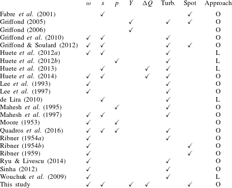
Selected studies carried out within these two general frameworks are listed in table 1 in an attempted summary, sorting the studies referred to in the two previous paragraphs according to the perturbation modes considered, the possibility of accounting for heat releasing/absorbing shock as well as the upstream perturbations and the approach followed. It is worth noting that in the case of an upstream turbulent field, LIA can be rewritten in terms of turbulent fluxes, leading to a linear problem for the jump of these quantities across the shock. These relations can be used to derive Reynolds-averaged Navier–Stokes (RANS) models well suited for the simulation of the shock–turbulence interaction (Sinha, Mahesh & Candler Reference Sinha, Mahesh and Candler2003; Griffond et al. Reference Griffond, Soulard and Souffland2010; Sinha Reference Sinha2012; Soulard, Griffond & Souffland Reference Soulard, Griffond and Souffland2012; Quadros et al. Reference Quadros, Sinha and Larsson2016).
Table 1. Summary of the LIA literature.
 $\unicode[STIX]{x1D714}$
,
$\unicode[STIX]{x1D714}$
,
 $s$
,
$s$
,
 $p$
and
$p$
and
 $Y$
indicate the considered incident Kovásznay modes, and
$Y$
indicate the considered incident Kovásznay modes, and
 $\unicode[STIX]{x0394}Q$
the presence of a heat releasing and/or absorbing shock. ‘Turb’ (turbulent) and ‘Spot’ refer to the nature of the upstream field. The approach followed is also indicated as L/O, referring respectively studies articles based/not based on the Laplace transform.
$\unicode[STIX]{x0394}Q$
the presence of a heat releasing and/or absorbing shock. ‘Turb’ (turbulent) and ‘Spot’ refer to the nature of the upstream field. The approach followed is also indicated as L/O, referring respectively studies articles based/not based on the Laplace transform.
The goal of the present paper is threefold. First, it aims at providing a complete, unified formulation of the normal-mode-based LIA approach that encompasses all previous developments, namely a binary mixture of perfect gases interacting with a non-adiabatic shock wave considering the poloidal/toroidal splitting of vorticity. The various extensions mentioned above have not been gathered into a single unified framework up to now. In particular, accounting for the non-adiabatic character of a shock wave simultaneously with these extensions has not been done up to now, although it was carried out in the case of density fluctuations through detonations (Huete et al. Reference Huete, Sánchez and Williams2013, Reference Huete, Sánchez and Williams2014). Heat release/absorption will be described as a punctual source/sink at the shock, to encompass thin reactive shock waves, shock-induced condensation or radiative loss (see e.g. Zel’Dovich & Raizer Reference ZelDovich and Raizer2012). In this general formulation, all types of upstream disturbances will be considered within an extended Kovásznay decomposition framework.
The second goal of the paper is to extend Chu’s definition for disturbance energy (Chu Reference Chu1965) to a multi-component fluid: a physically relevant and mathematically consistent definition well suited for small perturbations definition of the disturbance energy is of primary importance to analyse the effect of the interaction with the shock wave, and is therefore a prerequisite to the present paper’s goal.
The last goal of the present paper is to analyse the interaction of a Gaussian perturbation spot with a shock wave in the presence of the phenomena mentioned above. Three different cases are investigated: a density spot, an entropy spot and a vorticity spot (i.e. a weak vortex). It is worth noting that the case of upstream density heterogeneities has been considered in the case of non-reactive shock waves and thin strong detonations by Huete et al. (Reference Huete, Sánchez and Williams2013). Such a simple configuration can be considered as an idealized model of the interaction of a shock wave with a two-phase heterogeneity (bubble, droplet) with small density ratio. To the knowledge of the authors, such general cases have never been considered in the open literature until now. Using the three elementary cases considered in the present paper, an infinite number of cases can be derived by linear combination of the LIA results. As an example, the interaction between a shock wave and a cold weak vortex is obtained in a straightforward way by linear combination of the solutions related to the isentropic vortex case and a cold entropy spot. Multiple spot solutions can also be found in the same way, introducing a space–time shift in the solution associated with each spot. The optimal combination of these elementary spots to minimize the radiated noise is investigated in the present paper.
The paper is organized as follows. The basic physical model and associated governing equations are displayed in § 2. The decomposition of both upstream and downstream fields according to the present extended Kovásznay modal decomposition is then presented in § 3. The extended definition of disturbance energy and its relation to the energy of Kovásznay modes are discussed in § 4. Then the proposed general formulation of the normal-mode-based LIA approach is discussed in § 5. The application to the interaction of a heat releasing/absorbing shock wave with a variety of Gaussian spots (for density, entropy and vorticity fluctuations) is then addressed in § 6, with most of the technical details regarding the treatment of two-dimensional (2-D) Gaussian spots given in appendix A. Conclusions are drawn in § 7.
2 Physical model
The physical model addressed in the present paper is related to the case of 2-D canonical shock/disturbance interaction in a binary mixture of perfect gases, in the presence of heat release/absorption on the shock wave. Viscous effects are neglected. Upstream and downstream of the normal shock, the flow is governed by the Euler equations,
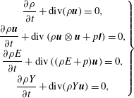 $$\begin{eqnarray}\left.\begin{array}{@{}c@{}}\displaystyle \frac{\unicode[STIX]{x2202}\unicode[STIX]{x1D70C}}{\unicode[STIX]{x2202}t}+\text{div}(\unicode[STIX]{x1D70C}\boldsymbol{u})=0,\\ \displaystyle \frac{\unicode[STIX]{x2202}\unicode[STIX]{x1D70C}\boldsymbol{u}}{\unicode[STIX]{x2202}t}+\text{div}\left(\unicode[STIX]{x1D70C}\boldsymbol{u}\otimes \boldsymbol{u}+p\unicode[STIX]{x1D644}\right)=0,\\ \displaystyle \frac{\unicode[STIX]{x2202}\unicode[STIX]{x1D70C}E}{\unicode[STIX]{x2202}t}+\text{div}\left((\unicode[STIX]{x1D70C}E+p)\boldsymbol{u}\right)=0,\\ \displaystyle \frac{\unicode[STIX]{x2202}\unicode[STIX]{x1D70C}Y}{\unicode[STIX]{x2202}t}+\text{div}(\unicode[STIX]{x1D70C}Y\boldsymbol{u})=0,\end{array}\right\}\end{eqnarray}$$
where
 $p,\unicode[STIX]{x1D70C},\boldsymbol{u}$
and
$p,\unicode[STIX]{x1D70C},\boldsymbol{u}$
and
 $E$
denote the mixture pressure, density, velocity and total energy; and
$E$
denote the mixture pressure, density, velocity and total energy; and
 $Y$
is the mass fraction of the first component in the binary mixture (see e.g. Williams Reference Williams1985).
$Y$
is the mass fraction of the first component in the binary mixture (see e.g. Williams Reference Williams1985).
The mixture equation of state for the binary mixture reads
 $$\begin{eqnarray}\displaystyle p=\unicode[STIX]{x1D70C}\frac{R}{W}T, & & \displaystyle\end{eqnarray}$$
where
 $R$
and
$R$
and
 $W$
denote the perfect gas constant and the molar weight of the mixture, respectively. The classical relations for ideal gas mixtures yield the following relations between the component properties and the mixture properties,
$W$
denote the perfect gas constant and the molar weight of the mixture, respectively. The classical relations for ideal gas mixtures yield the following relations between the component properties and the mixture properties,
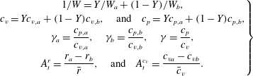 $$\begin{eqnarray}\displaystyle \left.\begin{array}{@{}c@{}}\displaystyle 1/W=Y/W_{a}+(1-Y)/W_{b},\\ \displaystyle c_{v}=Yc_{v,a}+(1-Y)c_{v,b},\quad \text{and}\quad c_{p}=Yc_{p,a}+(1-Y)c_{p,b},\\ \displaystyle \unicode[STIX]{x1D6FE}_{a}=\frac{c_{p,a}}{c_{v,a}},\quad \unicode[STIX]{x1D6FE}_{b}=\frac{c_{p,b}}{c_{v,b}},\quad \unicode[STIX]{x1D6FE}=\frac{c_{p}}{c_{v}},\\ \displaystyle A_{t}^{r}=\frac{r_{a}-r_{b}}{\bar{r}},\quad \text{and}\quad A_{t}^{c_{v}}=\frac{c_{va}-c_{vb}}{\bar{c}_{v}}.\end{array}\right\} & & \displaystyle\end{eqnarray}$$
 $W$
,
$W$
,
 $c_{v}$
,
$c_{v}$
,
 $c_{p}$
and
$c_{p}$
and
 $\unicode[STIX]{x1D6FE}$
denote respectively the mixture molecular weight, mass heat capacity at constant volume and constant pressure, the heat capacity ratio, as well as two Atwood numbers, to be used hereafter. Subscripts
$\unicode[STIX]{x1D6FE}$
denote respectively the mixture molecular weight, mass heat capacity at constant volume and constant pressure, the heat capacity ratio, as well as two Atwood numbers, to be used hereafter. Subscripts
 $a$
and
$a$
and
 $b$
denote the corresponding component thermodynamic properties in the binary mixture, one being inert and one possibly reactive. Note however that they do not intervene in the following, where indices exclusively serve as to identify the upstream and downstream states.
$b$
denote the corresponding component thermodynamic properties in the binary mixture, one being inert and one possibly reactive. Note however that they do not intervene in the following, where indices exclusively serve as to identify the upstream and downstream states.
Considering the case of a 1-D flow along the
 $x$
axis and a normal shock wave and denoting
$x$
axis and a normal shock wave and denoting
 $(u_{x},u_{r},u_{\unicode[STIX]{x1D719}})$
the components of velocity in cylindrical coordinates (in the discontinuity reference frame, the
$(u_{x},u_{r},u_{\unicode[STIX]{x1D719}})$
the components of velocity in cylindrical coordinates (in the discontinuity reference frame, the
 $x$
axis being taken normal to the planar shock wave), the upstream and downstream mean quantities (respectively subscripts 1, 2) are related through the Hugoniot jump conditions for mass, momentum and energy,
$x$
axis being taken normal to the planar shock wave), the upstream and downstream mean quantities (respectively subscripts 1, 2) are related through the Hugoniot jump conditions for mass, momentum and energy,
 $$\begin{eqnarray}\displaystyle \left.\begin{array}{@{}c@{}}\displaystyle \unicode[STIX]{x1D70C}_{1}u_{x1}=\unicode[STIX]{x1D70C}_{2}u_{x2},\\ \displaystyle p_{1}+\unicode[STIX]{x1D70C}_{1}u_{x1}^{2}=p_{2}+\unicode[STIX]{x1D70C}_{2}u_{x2}^{2},\\ \displaystyle h_{1}+\frac{u_{x1}^{2}}{2}=h_{2}+\frac{u_{x2}^{2}}{2},\end{array}\right\} & & \displaystyle\end{eqnarray}$$
with
 $u_{r}$
,
$u_{r}$
,
 $u_{\unicode[STIX]{x1D719}}$
and
$u_{\unicode[STIX]{x1D719}}$
and
 $Y_{a}$
being conserved through the shock
$Y_{a}$
being conserved through the shock
 $$\begin{eqnarray}u_{r1}=u_{r1},\quad u_{\unicode[STIX]{x1D719}1}=u_{\unicode[STIX]{x1D719}2},\quad Y_{a,1}=Y_{a,2}.\end{eqnarray}$$
The enthalpy
 $h$
jump condition may be reformulated as
$h$
jump condition may be reformulated as
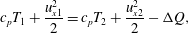 $$\begin{eqnarray}\displaystyle c_{p}T_{1}+\frac{u_{x1}^{2}}{2}=c_{p}T_{2}+\frac{u_{x2}^{2}}{2}-\unicode[STIX]{x0394}Q, & & \displaystyle\end{eqnarray}$$
where
 $\unicode[STIX]{x0394}Q$
accounts for heat release/heat absorption at the shock wave.
$\unicode[STIX]{x0394}Q$
accounts for heat release/heat absorption at the shock wave.
The case
 $\unicode[STIX]{x0394}Q>0$
was considered by Huete et al. (Reference Huete, Sánchez and Williams2013) to model thin detonations, while
$\unicode[STIX]{x0394}Q>0$
was considered by Huete et al. (Reference Huete, Sánchez and Williams2013) to model thin detonations, while
 $\unicode[STIX]{x0394}Q<0$
should be used to account for physical mechanisms restricted to a thin region downstream of the shock front that act as an energy sink, e.g. radiative losses or condensation (Zel’Dovich & Raizer Reference ZelDovich and Raizer2012).
$\unicode[STIX]{x0394}Q<0$
should be used to account for physical mechanisms restricted to a thin region downstream of the shock front that act as an energy sink, e.g. radiative losses or condensation (Zel’Dovich & Raizer Reference ZelDovich and Raizer2012).
Note that, while
 $\unicode[STIX]{x0394}Q$
is here formulated as an independent parameter, a classical assumption for strong detonations (see, e.g. Williams Reference Williams1985), the heat absorption typically depends on the shock strength for endothermic processes (which typically ends when saturation is reached), as is the case in ionizing, nuclear dissociating shocks such as those occurring in core collapsing supernovae (Abdikamalov et al.
Reference Abdikamalov, Huete, Nussupbekov and Berdibek2018; Huete, Abdikamalov & Radice Reference Huete, Abdikamalov and Radice2018; Huete & Abdikamalov Reference Huete and Abdikamalov2019), shock-induced condensation in vapour–liquid two-phase flow (Zhao et al.
Reference Zhao, Wang, Gao, Tang and Yuan2008) or cooling induced by radiative loss (Narita Reference Narita1973).
$\unicode[STIX]{x0394}Q$
is here formulated as an independent parameter, a classical assumption for strong detonations (see, e.g. Williams Reference Williams1985), the heat absorption typically depends on the shock strength for endothermic processes (which typically ends when saturation is reached), as is the case in ionizing, nuclear dissociating shocks such as those occurring in core collapsing supernovae (Abdikamalov et al.
Reference Abdikamalov, Huete, Nussupbekov and Berdibek2018; Huete, Abdikamalov & Radice Reference Huete, Abdikamalov and Radice2018; Huete & Abdikamalov Reference Huete and Abdikamalov2019), shock-induced condensation in vapour–liquid two-phase flow (Zhao et al.
Reference Zhao, Wang, Gao, Tang and Yuan2008) or cooling induced by radiative loss (Narita Reference Narita1973).
Introducing the sound speeds on either side of the shock
 $c_{1},c_{2}$
in the jump conditions leads to the following relation between the upstream and downstream Mach Numbers, respectively
$c_{1},c_{2}$
in the jump conditions leads to the following relation between the upstream and downstream Mach Numbers, respectively
 $M_{1}$
and
$M_{1}$
and
 $M_{2}$
,
$M_{2}$
,
 $$\begin{eqnarray}M_{2}^{2}=\frac{1+\unicode[STIX]{x1D6FE}M_{1}^{2}-(M_{1}^{2}-1)\sqrt{1-\unicode[STIX]{x1D6FD}}}{1+\unicode[STIX]{x1D6FE}M_{1}^{2}+\unicode[STIX]{x1D6FE}(M_{1}^{2}-1)\sqrt{1-\unicode[STIX]{x1D6FD}}},\quad \unicode[STIX]{x1D6FD}=\frac{2(\unicode[STIX]{x1D6FE}^{2}-1)M_{1}^{2}q}{(1-M_{1}^{2})^{2}},\end{eqnarray}$$
where the normalized heat coefficient has been introduced
 $$\begin{eqnarray}\displaystyle q=\frac{\unicode[STIX]{x0394}Q}{c_{1}^{2}}. & & \displaystyle\end{eqnarray}$$
The compression factor
 $m=\unicode[STIX]{x1D70C}_{2}/\unicode[STIX]{x1D70C}_{1}=u_{1}/u_{2}$
is obtained through
$m=\unicode[STIX]{x1D70C}_{2}/\unicode[STIX]{x1D70C}_{1}=u_{1}/u_{2}$
is obtained through
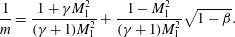 $$\begin{eqnarray}\frac{1}{m}=\frac{1+\unicode[STIX]{x1D6FE}M_{1}^{2}}{(\unicode[STIX]{x1D6FE}+1)M_{1}^{2}}+\frac{1-M_{1}^{2}}{(\unicode[STIX]{x1D6FE}+1)M_{1}^{2}}\sqrt{1-\unicode[STIX]{x1D6FD}}.\end{eqnarray}$$
Note that
 $c_{p}$
and
$c_{p}$
and
 $\unicode[STIX]{x1D6FE}$
appearing in the above relations are identical on both sides of the shock thanks to the continuity of mass fraction
$\unicode[STIX]{x1D6FE}$
appearing in the above relations are identical on both sides of the shock thanks to the continuity of mass fraction
 $Y$
, thereby considerably reducing the equations. A detailed account on the validity of this assumption has been provided by Griffond (Reference Griffond2005): the analysis is valid for small concentration fluctuations within binary mixtures with very different thermodynamic properties, or large concentration fluctuations within gases of similar thermodynamic properties. This translates, in practice, to the assumption holding when the reactive component mixture is sufficiently dilute in the inert one, as is often the case in air. When the assumption does not hold, the present study still presents valuable benchmarks for numerical codes, in which thermodynamic properties may be artificially set to constants.
$Y$
, thereby considerably reducing the equations. A detailed account on the validity of this assumption has been provided by Griffond (Reference Griffond2005): the analysis is valid for small concentration fluctuations within binary mixtures with very different thermodynamic properties, or large concentration fluctuations within gases of similar thermodynamic properties. This translates, in practice, to the assumption holding when the reactive component mixture is sufficiently dilute in the inert one, as is often the case in air. When the assumption does not hold, the present study still presents valuable benchmarks for numerical codes, in which thermodynamic properties may be artificially set to constants.
All other classical relations for
 $T_{2}/T_{1},p_{2}/p_{1},\ldots$
are formally identical to those of the classical normal shock case,
$T_{2}/T_{1},p_{2}/p_{1},\ldots$
are formally identical to those of the classical normal shock case,
 $M_{2}$
and
$M_{2}$
and
 $m$
being now given by the above formula.
$m$
being now given by the above formula.
The consistency constraint which ensures that both
 $m$
and
$m$
and
 $M_{2}$
remain positive is
$M_{2}$
remain positive is
 $$\begin{eqnarray}q_{min}<q<q_{max},\end{eqnarray}$$
where
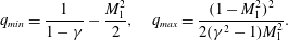 $$\begin{eqnarray}q_{min}=\frac{1}{1-\unicode[STIX]{x1D6FE}}-\frac{M_{1}^{2}}{2},\quad q_{max}=\frac{(1-M_{1}^{2})^{2}}{2(\unicode[STIX]{x1D6FE}^{2}-1)M_{1}^{2}}.\end{eqnarray}$$
The consistent domain for heat source/sink as a function of the upstream Mach number
 $M_{1}$
is illustrated in figure 1. Superimposed are contours of the downstream Mach number
$M_{1}$
is illustrated in figure 1. Superimposed are contours of the downstream Mach number
 $M_{2}$
, as provided by (2.7). One recovers the physical behaviour that the downstream flow is accelerated in the case
$M_{2}$
, as provided by (2.7). One recovers the physical behaviour that the downstream flow is accelerated in the case
 $q>0$
compared to the neutral shock case
$q>0$
compared to the neutral shock case
 $q=0$
, while it is decelerated in the opposite case
$q=0$
, while it is decelerated in the opposite case
 $q<0$
, due to the balance between kinetic energy and internal energy. In the asymptotic limit
$q<0$
, due to the balance between kinetic energy and internal energy. In the asymptotic limit
 $q=q_{max}$
, the system satisfies the so-called Chapman–Jouguet condition
$q=q_{max}$
, the system satisfies the so-called Chapman–Jouguet condition
 $M_{2}=1$
(see, e.g. Zeldovich Reference Zeldovich1950). The other limit,
$M_{2}=1$
(see, e.g. Zeldovich Reference Zeldovich1950). The other limit,
 $q=q_{min}$
corresponds to an infinite mass compression ratio, impossible to sustain in practice. For this reason, the endothermic cases presented in § 6 are presented for
$q=q_{min}$
corresponds to an infinite mass compression ratio, impossible to sustain in practice. For this reason, the endothermic cases presented in § 6 are presented for
 $q=q_{min}/2$
, translating to at most half the upstream kinetic energy being absorbed, leading to reasonable compression ratio and downstream Mach numbers (respectively
$q=q_{min}/2$
, translating to at most half the upstream kinetic energy being absorbed, leading to reasonable compression ratio and downstream Mach numbers (respectively
 $m=6.5$
and
$m=6.5$
and
 $M_{2}=0.33$
).
$M_{2}=0.33$
).


3 The Kovásznay modal decomposition for disturbances in a binary mixture of ideal gas
The linear interaction approximation relies on a small disturbance hypothesis and the use of linearized equations to described fluctuation propagation on either side of the shock.
For each quantity (e.g.
 $u$
), let us identify the fluctuation part (
$u$
), let us identify the fluctuation part (
 $u^{\prime }$
) and the mean (
$u^{\prime }$
) and the mean (
 $\bar{u}$
) as
$\bar{u}$
) as
 $$\begin{eqnarray}u=\bar{u}+u^{\prime },\quad p=\bar{p}+p^{\prime },\ldots\end{eqnarray}$$
and assume the fluctuation part is small (
 $u^{\prime }/\bar{u}\ll 1$
), a classical assumption provided:
$u^{\prime }/\bar{u}\ll 1$
), a classical assumption provided:
(i) Linearization of
 $Y$
, for which
$\bar{Y}=0$
is acceptable, is valid (Griffond Reference Griffond2005). This is in practice related to the continuity of
$c_{p}$
and
$\unicode[STIX]{x1D6FE}$
discussed after (2.9).
$Y$
, for which
$\bar{Y}=0$
is acceptable, is valid (Griffond Reference Griffond2005). This is in practice related to the continuity of
$c_{p}$
and
$\unicode[STIX]{x1D6FE}$
discussed after (2.9).(ii) Similarly, the linearization for the normal shock velocity is questionable in the limit
$\bar{u}\rightarrow 0$
, attainable when
$q\rightarrow q_{min}$
. To avoid this, the present study should not be carried out for
$M_{2}<0.25$
, or, alternatively,
$q<q_{min}/2$
.


In the reference frame tied to the planar shock front the 2-D perturbation field then satisfies
 $$\begin{eqnarray}\left.\begin{array}{@{}c@{}}\displaystyle \frac{\unicode[STIX]{x2202}\unicode[STIX]{x1D70C}^{\prime }}{\unicode[STIX]{x2202}t}+\bar{u}\frac{\unicode[STIX]{x2202}\unicode[STIX]{x1D70C}^{\prime }}{\unicode[STIX]{x2202}x}+\bar{\unicode[STIX]{x1D70C}}\frac{\unicode[STIX]{x2202}u_{j}^{\prime }}{\unicode[STIX]{x2202}x_{j}}=0,\\ \displaystyle \frac{\unicode[STIX]{x2202}u_{i}^{\prime }}{\unicode[STIX]{x2202}t}+\bar{u}\frac{\unicode[STIX]{x2202}u_{i}^{\prime }}{\unicode[STIX]{x2202}x}+\frac{1}{\bar{\unicode[STIX]{x1D70C}}}\frac{\unicode[STIX]{x2202}p^{\prime }}{\unicode[STIX]{x2202}x_{i}}=0,\\ \displaystyle \frac{\unicode[STIX]{x2202}Y^{\prime }}{\unicode[STIX]{x2202}t}+\bar{u}\frac{\unicode[STIX]{x2202}Y^{\prime }}{\unicode[STIX]{x2202}x}=0,\\ \displaystyle \frac{\unicode[STIX]{x2202}p^{\prime }}{\unicode[STIX]{x2202}t}+\bar{u}\frac{\unicode[STIX]{x2202}p^{\prime }}{\unicode[STIX]{x2202}x}+\unicode[STIX]{x1D6FE}\bar{p}\frac{\unicode[STIX]{x2202}u_{j}^{\prime }}{\unicode[STIX]{x2202}x_{j}}=0,\end{array}\right\}\end{eqnarray}$$
which can be recast as a system of evolution equations for Kovásznay’s physical modes,
 $$\begin{eqnarray}\left.\begin{array}{@{}c@{}}\displaystyle \frac{\unicode[STIX]{x2202}s^{\prime }}{\unicode[STIX]{x2202}t}+\bar{u}\frac{\unicode[STIX]{x2202}s^{\prime }}{\unicode[STIX]{x2202}x}=0,\\ \displaystyle \frac{\unicode[STIX]{x2202}\unicode[STIX]{x1D74E}_{\Vert }^{\prime }}{\unicode[STIX]{x2202}t}+\bar{u}\frac{\unicode[STIX]{x2202}\unicode[STIX]{x1D74E}_{\Vert }^{\prime }}{\unicode[STIX]{x2202}x}=0,\\ \displaystyle \frac{\unicode[STIX]{x2202}\unicode[STIX]{x1D74E}_{\bot }^{\prime }}{\unicode[STIX]{x2202}t}+\bar{u}\frac{\unicode[STIX]{x2202}\unicode[STIX]{x1D74E}_{\bot }^{\prime }}{\unicode[STIX]{x2202}x}=0,\\ \displaystyle \left(\frac{\unicode[STIX]{x2202}}{\unicode[STIX]{x2202}t}+\bar{u}\frac{\unicode[STIX]{x2202}}{\unicode[STIX]{x2202}x}\right)^{2}p^{\prime }=c^{2}\unicode[STIX]{x1D6FB}^{2}p^{\prime },\\ \displaystyle \frac{\unicode[STIX]{x2202}Y^{\prime }}{\unicode[STIX]{x2202}t}+\bar{u}\frac{\unicode[STIX]{x2202}Y^{\prime }}{\unicode[STIX]{x2202}x}=0,\end{array}\right\}\end{eqnarray}$$
where
 $\unicode[STIX]{x1D714}^{\prime }=\unicode[STIX]{x1D735}\times \boldsymbol{u}^{\prime }$
denotes the fluctuating vorticity, and
$\unicode[STIX]{x1D714}^{\prime }=\unicode[STIX]{x1D735}\times \boldsymbol{u}^{\prime }$
denotes the fluctuating vorticity, and
 $\unicode[STIX]{x1D74E}_{\bot }^{\prime }=(\unicode[STIX]{x1D714}^{\prime }\boldsymbol{\cdot }\boldsymbol{n})\boldsymbol{n}$
and
$\unicode[STIX]{x1D74E}_{\bot }^{\prime }=(\unicode[STIX]{x1D714}^{\prime }\boldsymbol{\cdot }\boldsymbol{n})\boldsymbol{n}$
and
 $\unicode[STIX]{x1D74E}_{\Vert }^{\prime }=\unicode[STIX]{x1D714}^{\prime }-\unicode[STIX]{x1D74E}_{\bot }^{\prime }$
are the shock-normal and the shock-parallel components of vorticity, respectively, with
$\unicode[STIX]{x1D74E}_{\Vert }^{\prime }=\unicode[STIX]{x1D714}^{\prime }-\unicode[STIX]{x1D74E}_{\bot }^{\prime }$
are the shock-normal and the shock-parallel components of vorticity, respectively, with
 $\boldsymbol{n}$
the unit normal vector of the planar shock wave. The shock-normal and the shock-tangential components correspond to the toroidal and poloidal components of the velocity field in the reference frame tied to the planar shock front, respectively.
$\boldsymbol{n}$
the unit normal vector of the planar shock wave. The shock-normal and the shock-tangential components correspond to the toroidal and poloidal components of the velocity field in the reference frame tied to the planar shock front, respectively.
One recognizes the entropy mode, the toroidal and poloidal vorticity modes, the fast and slow acoustic modes and the concentration mode. It is worth noting that Kovásznay’s modes correspond to the eigenmodes of the linearized propagation operator, which are orthonormal according to the inner product associated with Chu’s definition of compressible disturbance energy.
Let us now introduce propagating plane wave disturbances of the general form
 $$\begin{eqnarray}\unicode[STIX]{x1D719}^{\prime }=A_{i}(\boldsymbol{k})\exp [\text{i}(\boldsymbol{k}\boldsymbol{\cdot }\boldsymbol{x}-\unicode[STIX]{x1D6FA}t)].\end{eqnarray}$$
Here,
 $A_{i}(\boldsymbol{k})$
denotes the amplitude of upstream Kovásznay mode of type
$A_{i}(\boldsymbol{k})$
denotes the amplitude of upstream Kovásznay mode of type
 $i$
, with
$i$
, with
 $i=s,a,Y,v,t$
for the entropy, acoustic, concentration and poloidal/toroidal vorticity mode, respectively.
$i=s,a,Y,v,t$
for the entropy, acoustic, concentration and poloidal/toroidal vorticity mode, respectively.
 $\boldsymbol{k}$
is the perturbation wave vector, associated with pulsation
$\boldsymbol{k}$
is the perturbation wave vector, associated with pulsation
 $\unicode[STIX]{x1D6FA}=\bar{u}_{1}k\cos \unicode[STIX]{x1D6FC}$
, where
$\unicode[STIX]{x1D6FA}=\bar{u}_{1}k\cos \unicode[STIX]{x1D6FC}$
, where
 $\unicode[STIX]{x1D6FC}$
is the angle of the incident perturbation with respect to the shock, as illustrated in figure 2.
$\unicode[STIX]{x1D6FC}$
is the angle of the incident perturbation with respect to the shock, as illustrated in figure 2.
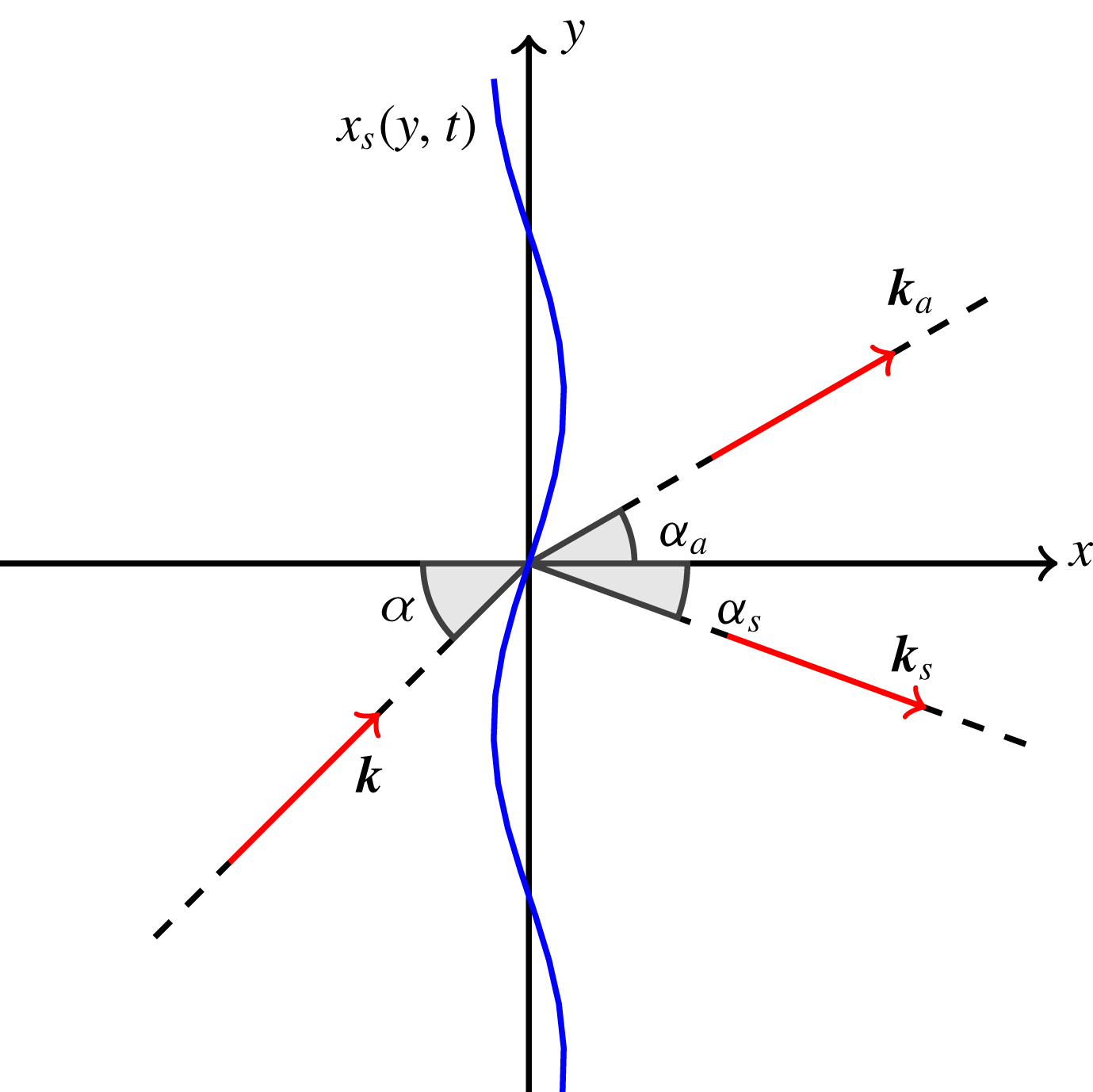
Figure 2. Sketch of the configuration. The corrugated shock mean front position is at
 $x=0$
. The incident perturbation has wave vector
$x=0$
. The incident perturbation has wave vector
 $\boldsymbol{k}$
, at angle
$\boldsymbol{k}$
, at angle
 $\unicode[STIX]{x1D6FC}$
with respect to the shock normal. Emitted waves may be acoustic waves, with wave vector
$\unicode[STIX]{x1D6FC}$
with respect to the shock normal. Emitted waves may be acoustic waves, with wave vector
 $\boldsymbol{k}_{a}$
, or non-acoustic ones, with wave vector
$\boldsymbol{k}_{a}$
, or non-acoustic ones, with wave vector
 $\boldsymbol{k}_{s}$
.
$\boldsymbol{k}_{s}$
.
The upstream fluctuating field can then be decomposed as follows
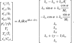 $$\begin{eqnarray}\left[\begin{array}{@{}c@{}}\unicode[STIX]{x1D70F}_{1}^{\prime }/\bar{\unicode[STIX]{x1D70F}}_{1}\\ u_{x1}^{\prime }/\bar{u}_{1}\\ u_{r1}^{\prime }/\bar{u}_{1}\\ u_{\unicode[STIX]{x1D719}1}^{\prime }/\bar{u}_{1}\\ p_{1}^{\prime }/\unicode[STIX]{x1D6FE}\bar{p}_{1}\\ Y_{1}^{\prime }\\ T_{1}^{\prime }/\bar{T}_{1}\\ s_{1}^{\prime }/C_{p1}\end{array}\right]=A_{i}(\boldsymbol{k})\text{e}^{\text{i}(\boldsymbol{k}\boldsymbol{\cdot }\boldsymbol{x}-\unicode[STIX]{x1D6FA}t)}\left[\begin{array}{@{}c@{}}\unicode[STIX]{x1D6FF}_{is}-\unicode[STIX]{x1D6FF}_{ia}+\unicode[STIX]{x1D6FF}_{iY}A_{t}^{r}\\ \unicode[STIX]{x1D6FF}_{iv}\sin \unicode[STIX]{x1D6FC}+\unicode[STIX]{x1D6FF}_{ia}{\displaystyle \frac{\cos \unicode[STIX]{x1D6FC}}{M_{1}}}\\ -\unicode[STIX]{x1D6FF}_{iv}\cos \unicode[STIX]{x1D6FC}+\unicode[STIX]{x1D6FF}_{ia}{\displaystyle \frac{\sin \unicode[STIX]{x1D6FC}}{M_{1}}}\\ \unicode[STIX]{x1D6FF}_{it}\\ \unicode[STIX]{x1D6FF}_{ia}\\ \unicode[STIX]{x1D6FF}_{iY}\\ \unicode[STIX]{x1D6FF}_{is}+(\unicode[STIX]{x1D6FE}-1)\unicode[STIX]{x1D6FF}_{ia}\\ \unicode[STIX]{x1D6FF}_{is}\end{array}\right],\end{eqnarray}$$
where
 $\unicode[STIX]{x1D6FF}_{ij}$
is the Kronecker symbol, and
$\unicode[STIX]{x1D6FF}_{ij}$
is the Kronecker symbol, and
 $\unicode[STIX]{x1D70F}=1/\unicode[STIX]{x1D70C}$
is the specific volume.
$\unicode[STIX]{x1D70F}=1/\unicode[STIX]{x1D70C}$
is the specific volume.
Now introducing the transfer function
 $Z_{ij}$
between upstream Kovásznay mode of type
$Z_{ij}$
between upstream Kovásznay mode of type
 $i$
and downstream Kovásznay mode of type
$i$
and downstream Kovásznay mode of type
 $j$
, the emitted fluctuating field downstream the shock is given by:
$j$
, the emitted fluctuating field downstream the shock is given by:
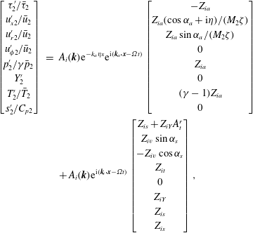 $$\begin{eqnarray}\displaystyle \left[\begin{array}{@{}c@{}}\unicode[STIX]{x1D70F}_{2}^{\prime }/\bar{\unicode[STIX]{x1D70F}}_{2}\\ u_{x2}^{\prime }/\bar{u}_{2}\\ u_{r2}^{\prime }/\bar{u}_{2}\\ u_{\unicode[STIX]{x1D719}2}^{\prime }/\bar{u}_{2}\\ p_{2}^{\prime }/\unicode[STIX]{x1D6FE}\bar{p}_{2}\\ Y_{2}^{\prime }\\ T_{2}^{\prime }/\bar{T}_{2}\\ s_{2}^{\prime }/C_{p2}\end{array}\right] & = & \displaystyle A_{i}(\boldsymbol{k})\text{e}^{-k_{a}\,\unicode[STIX]{x1D702}x}\text{e}^{\text{i}(\boldsymbol{k}_{a}\boldsymbol{\cdot }\boldsymbol{x}-\unicode[STIX]{x1D6FA}t)}\left[\begin{array}{@{}c@{}}-Z_{ia}\\ Z_{ia}(\cos \unicode[STIX]{x1D6FC}_{a}+\text{i}\unicode[STIX]{x1D702})/(M_{2}\unicode[STIX]{x1D701})\\ Z_{ia}\sin \unicode[STIX]{x1D6FC}_{a}/(M_{2}\unicode[STIX]{x1D701})\\ 0\\ Z_{ia}\\ 0\\ (\unicode[STIX]{x1D6FE}-1)Z_{ia}\\ 0\end{array}\right]\nonumber\\ \displaystyle & & \displaystyle +\,A_{i}(\boldsymbol{k})\text{e}^{\text{i}(\boldsymbol{k}_{s}\boldsymbol{\cdot }\boldsymbol{x}-\unicode[STIX]{x1D6FA}t)}\left[\begin{array}{@{}c@{}}Z_{is}+Z_{iY}A_{t}^{r}\\ Z_{iv}\sin \unicode[STIX]{x1D6FC}_{s}\\ -Z_{iv}\cos \unicode[STIX]{x1D6FC}_{s}\\ Z_{it}\\ 0\\ Z_{iY}\\ Z_{is}\\ Z_{is}\end{array}\right],\end{eqnarray}$$
where
 $$\begin{eqnarray}\displaystyle \unicode[STIX]{x1D701}=\sqrt{1-\unicode[STIX]{x1D702}^{2}+2\text{i}\unicode[STIX]{x1D702}\,\cos \unicode[STIX]{x1D6FC}_{a}}. & & \displaystyle\end{eqnarray}$$
Acoustic and non-acoustic emitted fluctuations are separated into two contributions in (3.6), as they correspond to different wave vectors, respectively
 $\boldsymbol{k}_{a}$
(possibly associated with attenuation
$\boldsymbol{k}_{a}$
(possibly associated with attenuation
 $\unicode[STIX]{x1D702}$
) and
$\unicode[STIX]{x1D702}$
) and
 $\boldsymbol{k}_{s}$
. These wave vectors are detailed hereafter. The transfer function
$\boldsymbol{k}_{s}$
. These wave vectors are detailed hereafter. The transfer function
 $Z_{ij}$
coefficients are explicitly given in § 5.
$Z_{ij}$
coefficients are explicitly given in § 5.
Emitted acoustic and non-acoustic wave vectors
Evaluation of the wave vectors
 $\boldsymbol{k}_{a}$
,
$\boldsymbol{k}_{a}$
,
 $\boldsymbol{k}_{s}$
and the associated angles
$\boldsymbol{k}_{s}$
and the associated angles
 $\unicode[STIX]{x1D6FC}_{a}$
,
$\unicode[STIX]{x1D6FC}_{a}$
,
 $\unicode[STIX]{x1D6FC}_{s}$
and attenuation
$\unicode[STIX]{x1D6FC}_{s}$
and attenuation
 $\unicode[STIX]{x1D702}$
is classical (see Fabre et al.
Reference Fabre, Jacquin and Sesterhenn2001; Sagaut & Cambon Reference Sagaut and Cambon2018), but is nonetheless recalled for the sake of completeness.
$\unicode[STIX]{x1D702}$
is classical (see Fabre et al.
Reference Fabre, Jacquin and Sesterhenn2001; Sagaut & Cambon Reference Sagaut and Cambon2018), but is nonetheless recalled for the sake of completeness.
The effect of
 $\unicode[STIX]{x1D6FC}$
being different whether the incident perturbation is acoustic (
$\unicode[STIX]{x1D6FC}$
being different whether the incident perturbation is acoustic (
 $i=a$
) or non-acoustic (
$i=a$
) or non-acoustic (
 $i\neq a$
), it is convenient to introduce the modified incident angle
$i\neq a$
), it is convenient to introduce the modified incident angle
 $\unicode[STIX]{x1D6FD}$
as
$\unicode[STIX]{x1D6FD}$
as
 $$\begin{eqnarray}\unicode[STIX]{x1D6FD}=\unicode[STIX]{x1D6FF}_{ia}\unicode[STIX]{x1D6FC}^{\prime }+(1-\unicode[STIX]{x1D6FF}_{ia})\unicode[STIX]{x1D6FC},\end{eqnarray}$$
where
 $\unicode[STIX]{x1D6FC}^{\prime }$
is defined as
$\unicode[STIX]{x1D6FC}^{\prime }$
is defined as
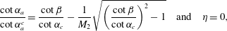
 $$\begin{eqnarray}\cot \unicode[STIX]{x1D6FC}^{\prime }=\cot \unicode[STIX]{x1D6FC}+\frac{1}{M_{1}\sin \unicode[STIX]{x1D6FC}}.\end{eqnarray}$$
Wave vectors and angles are then related through the relation:
 $$\begin{eqnarray}\displaystyle \frac{k_{a,s}}{k}=\frac{\sin \unicode[STIX]{x1D6FD}}{\sin \unicode[STIX]{x1D6FC}_{a,s}}, & & \displaystyle\end{eqnarray}$$
valid for both acoustic and non-acoustic emitted waves.
The emitted non-acoustic wave vector angle simply reads
 $$\begin{eqnarray}\cot \unicode[STIX]{x1D6FC}_{s}=m\,\cot \unicode[STIX]{x1D6FD},\end{eqnarray}$$
where
 $m$
is the compression factor (2.9).
$m$
is the compression factor (2.9).
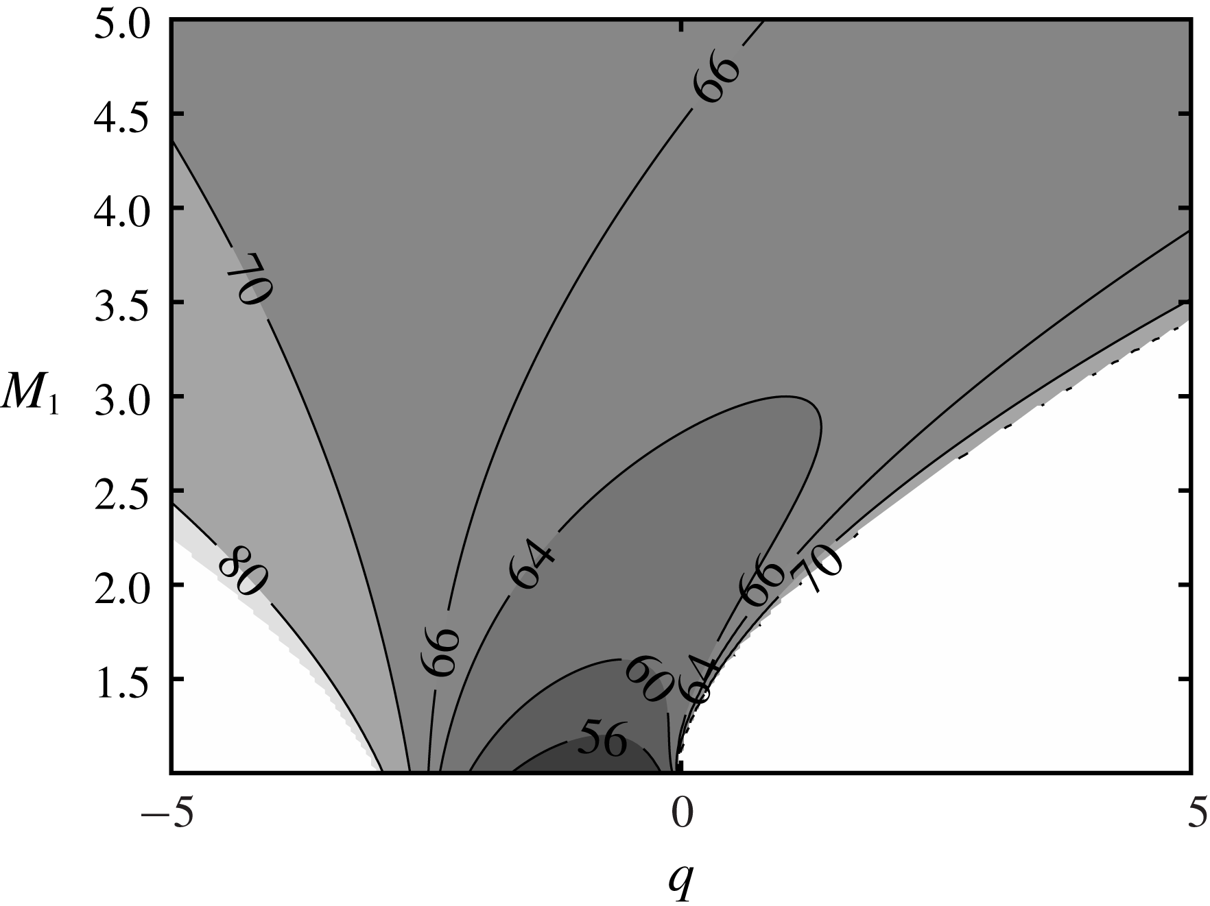
Figure 3. Isovalues of the critical angle
 $\unicode[STIX]{x1D6FC}_{c}$
as a function of the upstream Mach number
$\unicode[STIX]{x1D6FC}_{c}$
as a function of the upstream Mach number
 $M_{1}$
and the heat source term
$M_{1}$
and the heat source term
 $q$
. White areas correspond to unphysical configurations that violate the realizability constraint on the downstream flow.
$q$
. White areas correspond to unphysical configurations that violate the realizability constraint on the downstream flow.
Obtaining the emitted acoustic wave vector
 $\boldsymbol{k}_{a}$
and associated attenuation
$\boldsymbol{k}_{a}$
and associated attenuation
 $\unicode[STIX]{x1D702}$
is not as straightforward. If the incident perturbation is non-acoustic (
$\unicode[STIX]{x1D702}$
is not as straightforward. If the incident perturbation is non-acoustic (
 $i\neq a$
), a singularity appears for
$i\neq a$
), a singularity appears for
 $\unicode[STIX]{x1D6FC}=\unicode[STIX]{x1D6FD}=\unicode[STIX]{x1D6FC}_{c}$
, where
$\unicode[STIX]{x1D6FC}=\unicode[STIX]{x1D6FD}=\unicode[STIX]{x1D6FC}_{c}$
, where
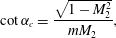 $$\begin{eqnarray}\cot \unicode[STIX]{x1D6FC}_{c}=\frac{\sqrt{1-M_{2}^{2}}}{mM_{2}},\end{eqnarray}$$
for which the emitted acoustic wave vector corresponds to the critical emission angle
 $$\begin{eqnarray}\cos \unicode[STIX]{x1D6FC}_{a}^{c}=-M_{2}.\end{eqnarray}$$
Contours of critical angle values (3.12) are given in figure 3 as a function of
 $M_{1}$
and
$M_{1}$
and
 $q$
.
$q$
.
If
 $\unicode[STIX]{x1D6FC}<\unicode[STIX]{x1D6FC}_{c}$
, the emitted wave vector angle reads
$\unicode[STIX]{x1D6FC}<\unicode[STIX]{x1D6FC}_{c}$
, the emitted wave vector angle reads
 $$\begin{eqnarray}\frac{\cot \unicode[STIX]{x1D6FC}_{a}}{\cot \unicode[STIX]{x1D6FC}_{a}^{c}}=\frac{\cot \unicode[STIX]{x1D6FD}}{\cot \unicode[STIX]{x1D6FC}_{c}}-\frac{1}{M_{2}}\sqrt{\left(\frac{\cot \unicode[STIX]{x1D6FD}}{\cot \unicode[STIX]{x1D6FC}_{c}}\right)^{2}-1}\quad \text{and}\quad \unicode[STIX]{x1D702}=0,\end{eqnarray}$$
else if
 $\unicode[STIX]{x1D6FC}>\unicode[STIX]{x1D6FC}_{c}$
:
$\unicode[STIX]{x1D6FC}>\unicode[STIX]{x1D6FC}_{c}$
:
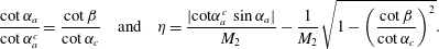 $$\begin{eqnarray}\frac{\cot \unicode[STIX]{x1D6FC}_{a}}{\cot \unicode[STIX]{x1D6FC}_{a}^{c}}=\frac{\cot \unicode[STIX]{x1D6FD}}{\cot \unicode[STIX]{x1D6FC}_{c}}\quad \text{and}\quad \unicode[STIX]{x1D702}=\frac{|\text{cot}\unicode[STIX]{x1D6FC}_{a}^{c}\,\sin \unicode[STIX]{x1D6FC}_{a}|}{M_{2}}-\frac{1}{M_{2}}\sqrt{1-\left(\frac{\cot \unicode[STIX]{x1D6FD}}{\cot \unicode[STIX]{x1D6FC}_{c}}\right)^{2}}.\end{eqnarray}$$
In the particular case where the incident perturbation is acoustic (
 $i=a$
),
$i=a$
),
 $\unicode[STIX]{x1D6FD}=\unicode[STIX]{x1D6FC}^{\prime }$
, and two critical values for the incident angle
$\unicode[STIX]{x1D6FD}=\unicode[STIX]{x1D6FC}^{\prime }$
, and two critical values for the incident angle
 $\unicode[STIX]{x1D6FC}$
are found,
$\unicode[STIX]{x1D6FC}$
are found,
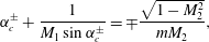 $$\begin{eqnarray}\unicode[STIX]{x1D6FC}_{c}^{\pm }+\frac{1}{M_{1}\sin \unicode[STIX]{x1D6FC}_{c}^{\pm }}=\mp \frac{\sqrt{1-M_{2}^{2}}}{mM_{2}},\end{eqnarray}$$
corresponding to fast and slow propagation regimes, separated by incident angle
 $\unicode[STIX]{x1D6FC}_{M}$
such as
$\unicode[STIX]{x1D6FC}_{M}$
such as
 $$\begin{eqnarray}\cos \unicode[STIX]{x1D6FC}_{M}=-\frac{1}{M_{1}}.\end{eqnarray}$$
For acoustic incident perturbations (
 $\unicode[STIX]{x1D6FD}=\unicode[STIX]{x1D6FC}^{\prime }$
) (3.14) and (3.15) remain valid, now defining four regimes: a propagating and non-propagating regime for each of the fast and slow modes.
$\unicode[STIX]{x1D6FD}=\unicode[STIX]{x1D6FC}^{\prime }$
) (3.14) and (3.15) remain valid, now defining four regimes: a propagating and non-propagating regime for each of the fast and slow modes.
The global procedure for the determination of emitted wave vectors as well as associated attenuation is summarized in table 2 and the resulting dependence on the incident angle is illustrated in figure 4.
Table 2. Computation of the emitted acoustic and non-acoustic wave vectors through the corresponding angles
 $\unicode[STIX]{x1D6FC}_{a}$
and
$\unicode[STIX]{x1D6FC}_{a}$
and
 $\unicode[STIX]{x1D6FC}_{s}$
, for non-acoustic and acoustic incident perturbations. Also included is the determination of attenuation
$\unicode[STIX]{x1D6FC}_{s}$
, for non-acoustic and acoustic incident perturbations. Also included is the determination of attenuation
 $\unicode[STIX]{x1D702}$
for the emitted acoustic waves.
$\unicode[STIX]{x1D702}$
for the emitted acoustic waves.
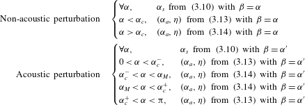
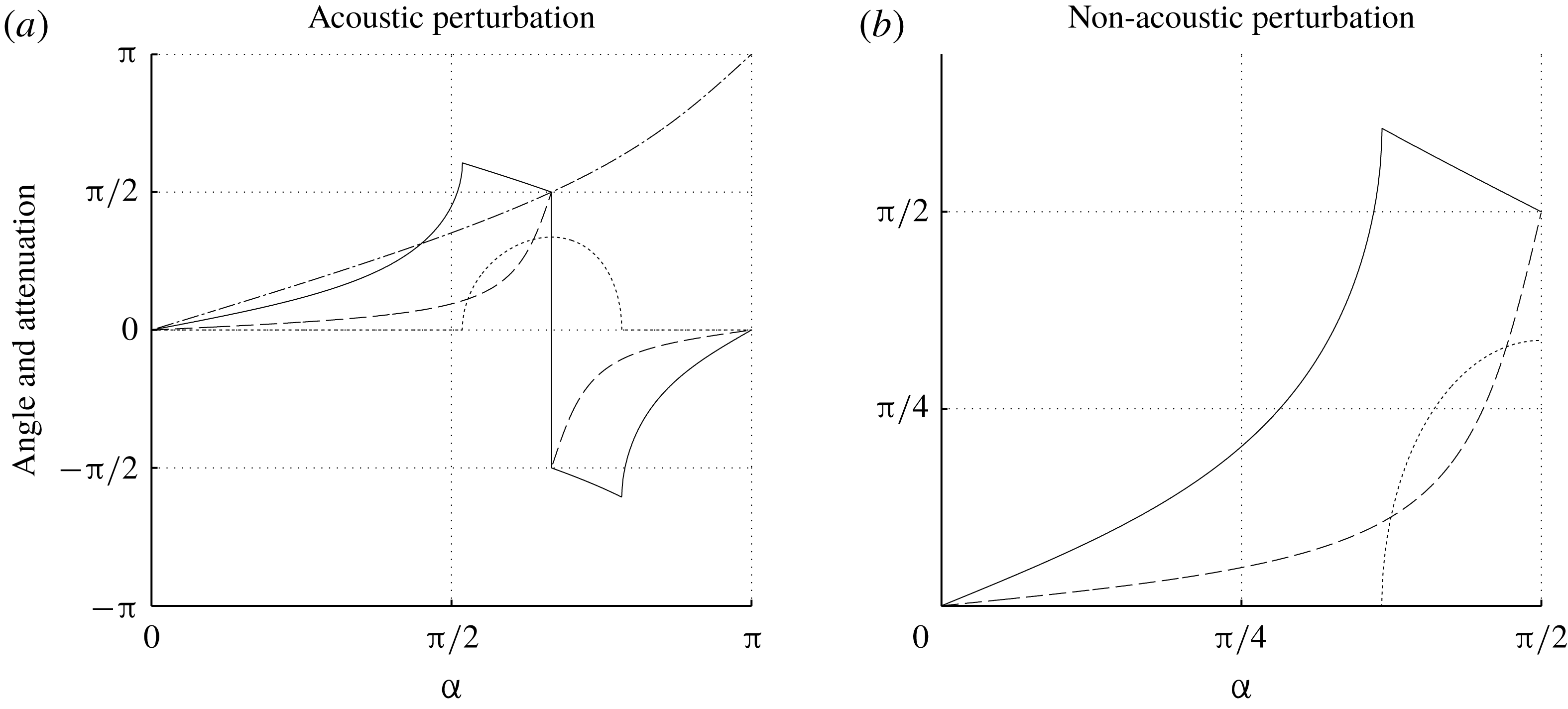
Figure 4. Emission angles and attenuation factor
 $\unicode[STIX]{x1D702}$
, obtained following the procedure summarized in table 2, for
$\unicode[STIX]{x1D702}$
, obtained following the procedure summarized in table 2, for
 $\unicode[STIX]{x1D6FE}=1.4$
,
$\unicode[STIX]{x1D6FE}=1.4$
,
 $M_{1}=2$
and
$M_{1}=2$
and
 $q=-2.25$
. Plain line:
$q=-2.25$
. Plain line:
 $\unicode[STIX]{x1D6FC}_{a}$
, dashed-line:
$\unicode[STIX]{x1D6FC}_{a}$
, dashed-line:
 $\unicode[STIX]{x1D6FC}_{s}$
, dotted line: attenuation
$\unicode[STIX]{x1D6FC}_{s}$
, dotted line: attenuation
 $\unicode[STIX]{x1D702}$
. In (a), the additional dot-dashed line represents the nonlinear dependence of
$\unicode[STIX]{x1D702}$
. In (a), the additional dot-dashed line represents the nonlinear dependence of
 $\unicode[STIX]{x1D6FD}$
as a function of
$\unicode[STIX]{x1D6FD}$
as a function of
 $\unicode[STIX]{x1D6FC}$
(3.8) in the case of an acoustic incident perturbation.
$\unicode[STIX]{x1D6FC}$
(3.8) in the case of an acoustic incident perturbation.
4 Extension of Chu’s definition for disturbance energy to a multi-component gas
An important issue is the derivation of a physically relevant and mathematically consistent definition of the energy of the disturbances in compressible flows. Chu’s definition (Chu Reference Chu1965) for the disturbance energy around a base flow has the advantage of defining an inner product, with respect to which the linearized Euler equations about a uniform base flow are self-adjoint, and Kovásznay modes correspond to orthogonal eigenmodes of the linearized operator. The orthogonality of eigenmodes prevents spurious non-normality-induced phenomenon in the computation of the energy of the fluctuating field (George & Sujith Reference George and Sujith2011; Sagaut & Cambon Reference Sagaut and Cambon2018). As a matter of fact, the use of a non-normal basis may lead to unphysical growth of the energy of the system because of the contributions of non-zero cross-products of basis vectors. Therefore, one can split the total energy as the sum
 $E_{tot}=\sum _{i}E_{i}$
, with
$E_{tot}=\sum _{i}E_{i}$
, with
 $i=v,a,s$
for the vorticity mode, the acoustic mode and the entropy mode, respectively.
$i=v,a,s$
for the vorticity mode, the acoustic mode and the entropy mode, respectively.
Since the present work deals with a multi-component gas, Chu’s original definition is extended in the present section. A first step consists of finding an expression for the linearized Euler equations that will lead to orthogonal eigenvectors. This is the case when the matrix associated with the linearized problem is symmetric. To this end, an adequate choice of physical unknowns must be done. Noticing that the set
 $(\unicode[STIX]{x1D70C},u,v,T,Y)$
leads to a non-symmetric matrix and non-orthogonal eigenvectors, we choose here to write the linearized problem using
$(\unicode[STIX]{x1D70C},u,v,T,Y)$
leads to a non-symmetric matrix and non-orthogonal eigenvectors, we choose here to write the linearized problem using
 $(\unicode[STIX]{x1D70C}_{a},\unicode[STIX]{x1D70C}_{b},u,v,T)$
,
$(\unicode[STIX]{x1D70C}_{a},\unicode[STIX]{x1D70C}_{b},u,v,T)$
,
 $$\begin{eqnarray}\left.\begin{array}{@{}c@{}}\displaystyle \frac{\unicode[STIX]{x2202}\unicode[STIX]{x1D70C}_{a}^{\prime }}{\unicode[STIX]{x2202}t}+\bar{u}\frac{\unicode[STIX]{x2202}\unicode[STIX]{x1D70C}_{a}^{\prime }}{\unicode[STIX]{x2202}x}+\bar{\unicode[STIX]{x1D70C}}_{a}\frac{\unicode[STIX]{x2202}u_{j}^{\prime }}{\unicode[STIX]{x2202}x_{j}}=0,\\ \displaystyle \frac{\unicode[STIX]{x2202}\unicode[STIX]{x1D70C}_{b}^{\prime }}{\unicode[STIX]{x2202}t}+\bar{u}\frac{\unicode[STIX]{x2202}\unicode[STIX]{x1D70C}_{b}^{\prime }}{\unicode[STIX]{x2202}x}+\bar{\unicode[STIX]{x1D70C}}_{b}\frac{\unicode[STIX]{x2202}u_{j}^{\prime }}{\unicode[STIX]{x2202}x_{j}}=0,\\ \displaystyle \frac{\unicode[STIX]{x2202}u_{i}^{\prime }}{\unicode[STIX]{x2202}t}+\bar{u}\frac{\unicode[STIX]{x2202}u_{i}^{\prime }}{\unicode[STIX]{x2202}x}+\frac{1}{\bar{\unicode[STIX]{x1D70C}}}\frac{\unicode[STIX]{x2202}p^{\prime }}{\unicode[STIX]{x2202}x_{i}}=0,\\ \displaystyle \frac{\unicode[STIX]{x2202}T^{\prime }}{\unicode[STIX]{x2202}t}+\bar{u}\frac{\unicode[STIX]{x2202}T^{\prime }}{\unicode[STIX]{x2202}x}+\frac{\bar{p}}{\bar{\unicode[STIX]{x1D70C}}C_{v}}\frac{\unicode[STIX]{x2202}u_{j}^{\prime }}{\unicode[STIX]{x2202}x_{j}}=0,\\ \displaystyle \frac{p^{\prime }}{\bar{p}}-\frac{T^{\prime }}{\bar{T}}-[1+A_{t}^{r}(1-Y_{0})]\frac{\unicode[STIX]{x1D70C}_{a}^{\prime }}{\unicode[STIX]{x1D70C}_{0}}-(1-A_{t}^{r}Y_{0})\frac{\unicode[STIX]{x1D70C}_{b}^{\prime }}{\unicode[STIX]{x1D70C}_{0}}=0,\end{array}\right\}\end{eqnarray}$$
where the last line is related to the linearized equation of state, with
 $$\begin{eqnarray}\displaystyle \unicode[STIX]{x1D70C}_{a}=\unicode[STIX]{x1D70C}Y,\quad \unicode[STIX]{x1D70C}_{b}=\unicode[STIX]{x1D70C}(1-Y), & & \displaystyle\end{eqnarray}$$
 $$\begin{eqnarray}\displaystyle & \displaystyle \frac{\unicode[STIX]{x1D70C}_{a}^{\prime }}{\unicode[STIX]{x1D70C}_{0}}=\frac{\unicode[STIX]{x1D70C}^{\prime }}{\unicode[STIX]{x1D70C}_{0}}Y_{0}+Y^{\prime }, & \displaystyle\end{eqnarray}$$
 $$\begin{eqnarray}\displaystyle & \displaystyle \frac{\unicode[STIX]{x1D70C}_{b}^{\prime }}{\unicode[STIX]{x1D70C}_{0}}=\frac{\unicode[STIX]{x1D70C}^{\prime }}{\unicode[STIX]{x1D70C}_{0}}(1-Y_{0})-Y^{\prime }. & \displaystyle\end{eqnarray}$$
Now introducing the vector of normalized variables
 $X=(\tilde{\unicode[STIX]{x1D70C}_{a}},\tilde{\unicode[STIX]{x1D70C}_{b}},\tilde{u} ,\tilde{v},\tilde{T})^{\text{T}}$
where
$X=(\tilde{\unicode[STIX]{x1D70C}_{a}},\tilde{\unicode[STIX]{x1D70C}_{b}},\tilde{u} ,\tilde{v},\tilde{T})^{\text{T}}$
where
 $$\begin{eqnarray}\left.\begin{array}{@{}c@{}}\tilde{u} ={\displaystyle \frac{u^{\prime }}{c_{0}}};\quad \tilde{v}={\displaystyle \frac{v^{\prime }}{c_{0}}};\quad \tilde{T}={\displaystyle \frac{T^{\prime }}{T_{0}\sqrt{\unicode[STIX]{x1D6FE}(\unicode[STIX]{x1D6FE}-1)}}};\\ \tilde{\unicode[STIX]{x1D70C}_{a}}={\displaystyle \frac{\unicode[STIX]{x1D70C}_{a}^{\prime }}{\unicode[STIX]{x1D70C}_{0}\sqrt{\displaystyle \frac{\unicode[STIX]{x1D6FE}Y_{0}}{1+A_{t}^{r}(1-Y_{0})}}}};\quad \tilde{\unicode[STIX]{x1D70C}_{b}}={\displaystyle \frac{\unicode[STIX]{x1D70C}_{b}^{\prime }}{\unicode[STIX]{x1D70C}_{0}\sqrt{\displaystyle \frac{\unicode[STIX]{x1D6FE}(1-Y_{0})}{1-A_{t}^{r}Y_{0}}}}}\end{array}\right\}\end{eqnarray}$$
and considering propagating plane wave disturbances, the linearized problem (4.1) can be rewritten in the following compact form
 $$\begin{eqnarray}\frac{\text{d}X}{\text{d}t}=\unicode[STIX]{x1D648}X,\end{eqnarray}$$
where the linearized operator matrix is given by
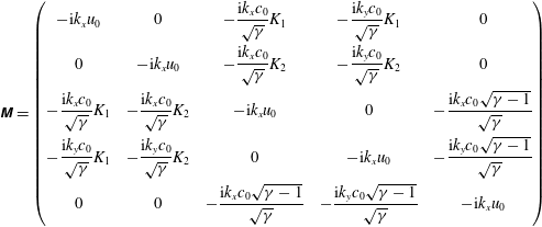 $$\begin{eqnarray}\displaystyle \unicode[STIX]{x1D648}=\left(\begin{array}{@{}ccccc@{}}-\text{i}k_{x}u_{0} & 0 & -{\displaystyle \frac{\text{i}k_{x}c_{0}}{\sqrt{\unicode[STIX]{x1D6FE}}}}K_{1} & -{\displaystyle \frac{\text{i}k_{y}c_{0}}{\sqrt{\unicode[STIX]{x1D6FE}}}}K_{1} & 0\\ 0 & -\text{i}k_{x}u_{0} & -{\displaystyle \frac{\text{i}k_{x}c_{0}}{\sqrt{\unicode[STIX]{x1D6FE}}}}K_{2} & -{\displaystyle \frac{\text{i}k_{y}c_{0}}{\sqrt{\unicode[STIX]{x1D6FE}}}}K_{2} & 0\\ -{\displaystyle \frac{\text{i}k_{x}c_{0}}{\sqrt{\unicode[STIX]{x1D6FE}}}}K_{1} & -{\displaystyle \frac{\text{i}k_{x}c_{0}}{\sqrt{\unicode[STIX]{x1D6FE}}}}K_{2} & -\text{i}k_{x}u_{0} & 0 & -{\displaystyle \frac{\text{i}k_{x}c_{0}\sqrt{\unicode[STIX]{x1D6FE}-1}}{\sqrt{\unicode[STIX]{x1D6FE}}}}\\ -{\displaystyle \frac{\text{i}k_{y}c_{0}}{\sqrt{\unicode[STIX]{x1D6FE}}}}K_{1} & -{\displaystyle \frac{\text{i}k_{y}c_{0}}{\sqrt{\unicode[STIX]{x1D6FE}}}}K_{2} & 0 & -\text{i}k_{x}u_{0} & -{\displaystyle \frac{\text{i}k_{y}c_{0}\sqrt{\unicode[STIX]{x1D6FE}-1}}{\sqrt{\unicode[STIX]{x1D6FE}}}}\\ 0 & 0 & -{\displaystyle \frac{\text{i}k_{x}c_{0}\sqrt{\unicode[STIX]{x1D6FE}-1}}{\sqrt{\unicode[STIX]{x1D6FE}}}} & -{\displaystyle \frac{\text{i}k_{y}c_{0}\sqrt{\unicode[STIX]{x1D6FE}-1}}{\sqrt{\unicode[STIX]{x1D6FE}}}} & -\text{i}k_{x}u_{0}\end{array}\right) & & \displaystyle \nonumber\\ \displaystyle & & \displaystyle\end{eqnarray}$$
where the two positive parameters
 $K_{1}$
and
$K_{1}$
and
 $K_{2}$
are defined as
$K_{2}$
are defined as
 $$\begin{eqnarray}K_{1}=\sqrt{Y_{0}[1+A_{t}^{r}(1-Y_{0})]},\quad K_{2}=\sqrt{(1-Y_{0})(1-A_{t}^{r}Y_{0})}.\end{eqnarray}$$
The five eigenvalues are
 $$\begin{eqnarray}-\text{i}k_{x}u_{0},\quad -\text{i}k_{x}u_{0},\quad -\text{i}k_{x}u_{0},\quad -\text{i}(k_{x}u_{0}\mp kc_{0}),\end{eqnarray}$$
which correspond to the normalized propagation speeds of (from the left to the right) the entropy mode, the vorticity mode, the concentration mode and the fast and slow acoustic modes. The associated set of orthogonal eigenvectors is
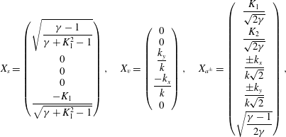 $$\begin{eqnarray}X_{s}=\left(\begin{array}{@{}c@{}}\sqrt{{\displaystyle \frac{\unicode[STIX]{x1D6FE}-1}{\unicode[STIX]{x1D6FE}+K_{1}^{2}-1}}}\\ 0\\ 0\\ 0\\ {\displaystyle \frac{-K_{1}}{\sqrt{\unicode[STIX]{x1D6FE}+K_{1}^{2}-1}}}\end{array}\right),\quad X_{v}=\left(\begin{array}{@{}c@{}}0\\ 0\\ {\displaystyle \frac{k_{y}}{k}}\\ {\displaystyle \frac{-k_{x}}{k}}\\ 0\end{array}\right),\quad X_{a^{\pm }}=\left(\begin{array}{@{}c@{}}{\displaystyle \frac{K_{1}}{\sqrt{2\unicode[STIX]{x1D6FE}}}}\\ {\displaystyle \frac{K_{2}}{\sqrt{2\unicode[STIX]{x1D6FE}}}}\\ {\displaystyle \frac{\pm k_{x}}{k\sqrt{2}}}\\ {\displaystyle \frac{\pm k_{y}}{k\sqrt{2}}}\\ \sqrt{{\displaystyle \frac{\unicode[STIX]{x1D6FE}-1}{2\unicode[STIX]{x1D6FE}}}}\\ \end{array}\right),\end{eqnarray}$$
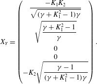 $$\begin{eqnarray}X_{Y}=\left(\begin{array}{@{}c@{}}{\displaystyle \frac{-K_{1}K_{2}}{\sqrt{(\unicode[STIX]{x1D6FE}+K_{1}^{2}-1)\unicode[STIX]{x1D6FE}}}}\\ \sqrt{{\displaystyle \frac{\unicode[STIX]{x1D6FE}+K_{1}^{2}-1}{\unicode[STIX]{x1D6FE}}}}\\ 0\\ 0\\ -K_{2}\sqrt{{\displaystyle \frac{\unicode[STIX]{x1D6FE}-1}{(\unicode[STIX]{x1D6FE}+K_{1}^{2}-1)\unicode[STIX]{x1D6FE}}}}\end{array}\right).\end{eqnarray}$$
All possible solutions of the linearized problem can be expressed as a linear combination of the eigenvectors:
 $X(t)=\sum _{i=s,v,a^{\pm },Y}C_{i}(t)X_{i}$
. Therefore a local definition of the total energy
$X(t)=\sum _{i=s,v,a^{\pm },Y}C_{i}(t)X_{i}$
. Therefore a local definition of the total energy
 $E(t)$
of the disturbance is given by the square of
$E(t)$
of the disturbance is given by the square of
 $L_{2}$
norm of
$L_{2}$
norm of
 $X(t)$
. Thanks to the orthogonality property, one has
$X(t)$
. Thanks to the orthogonality property, one has
 $\Vert X(t)\Vert ^{2}=X(t)\cdot X(t)=\sum _{i=s,v,a^{\pm },Y}C_{i}^{2}(t)\Vert X_{i}\Vert ^{2}$
, which appears as the sum of the energy of each mode. The associated energy in a volume
$\Vert X(t)\Vert ^{2}=X(t)\cdot X(t)=\sum _{i=s,v,a^{\pm },Y}C_{i}^{2}(t)\Vert X_{i}\Vert ^{2}$
, which appears as the sum of the energy of each mode. The associated energy in a volume
 $V$
is obtained in a straightforward way as
$V$
is obtained in a straightforward way as
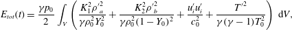 $$\begin{eqnarray}\displaystyle E_{tot}(t)=\frac{\unicode[STIX]{x1D6FE}p_{0}}{2}\int _{V}\left(\frac{K_{1}^{2}{\unicode[STIX]{x1D70C}^{\prime }}_{a}^{2}}{\unicode[STIX]{x1D6FE}\unicode[STIX]{x1D70C}_{0}^{2}Y_{0}^{2}}+\frac{K_{2}^{2}{\unicode[STIX]{x1D70C}^{\prime }}_{b}^{2}}{\unicode[STIX]{x1D6FE}\unicode[STIX]{x1D70C}_{0}^{2}(1-Y_{0})^{2}}+\frac{u_{i}^{\prime }u_{i}^{\prime }}{c_{0}^{2}}+\frac{{T^{\prime }}^{2}}{\unicode[STIX]{x1D6FE}(\unicode[STIX]{x1D6FE}-1)T_{0}^{2}}\right)\,\text{d}V, & & \displaystyle\end{eqnarray}$$
which can be rewritten as a function of
 $u_{i}^{\prime }$
,
$u_{i}^{\prime }$
,
 $p^{\prime }$
,
$p^{\prime }$
,
 $s^{\prime }$
and
$s^{\prime }$
and
 $Y^{\prime }$
as follows:
$Y^{\prime }$
as follows:
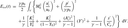 $$\begin{eqnarray}\displaystyle E_{tot}(t) & = & \displaystyle \frac{\unicode[STIX]{x1D6FE}p_{0}}{2}\int _{V}\left\{M_{0}^{2}\left(\frac{u_{i}^{\prime }}{u_{0}}\right)^{2}+\left(\frac{p^{\prime }}{\unicode[STIX]{x1D6FE}p_{0}}\right)^{2}\right.\nonumber\\ \displaystyle & & \displaystyle +\frac{1}{\unicode[STIX]{x1D6FE}}\left[\frac{K_{1}^{2}}{Y_{0}^{2}}+\frac{K_{2}^{2}}{(1-Y_{0})^{2}}+\frac{(A_{t}^{r})^{2}}{\unicode[STIX]{x1D6FE}-1}\right](Y^{\prime })^{2}+\left.\frac{1}{\unicode[STIX]{x1D6FE}-1}\left(\frac{s^{\prime }}{C_{p}}\right)^{2}\right\}\,\text{d}V.\end{eqnarray}$$
The original formula given by Chu for single-species fluids is recovered taking
 $Y_{0}=1$
(which leads to
$Y_{0}=1$
(which leads to
 $K_{1}=1$
,
$K_{1}=1$
,
 $K_{2}=0$
) along with
$K_{2}=0$
) along with
 $Y^{\prime }=0$
.
$Y^{\prime }=0$
.
5 A general formulation of the normal-mode-based LIA
The shock jump relations for a normal planar shock wave with possible heat release/absorption and change in specific heats across the shock read
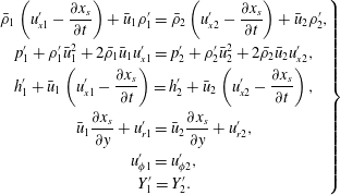 $$\begin{eqnarray}\displaystyle \left.\begin{array}{@{}c@{}}\displaystyle \bar{\unicode[STIX]{x1D70C}}_{1}\left(u_{x1}^{\prime }-\frac{\unicode[STIX]{x2202}x_{s}}{\unicode[STIX]{x2202}t}\right)+\bar{u}_{1}\unicode[STIX]{x1D70C}_{1}^{\prime }=\bar{\unicode[STIX]{x1D70C}}_{2}\left(u_{x2}^{\prime }-\frac{\unicode[STIX]{x2202}x_{s}}{\unicode[STIX]{x2202}t}\right)+\bar{u}_{2}\unicode[STIX]{x1D70C}_{2}^{\prime },\\ \displaystyle p_{1}^{\prime }+\unicode[STIX]{x1D70C}_{1}^{\prime }\bar{u}_{1}^{2}+2\bar{\unicode[STIX]{x1D70C}}_{1}\bar{u}_{1}u_{x1}^{\prime }=p_{2}^{\prime }+\unicode[STIX]{x1D70C}_{2}^{\prime }\bar{u}_{2}^{2}+2\bar{\unicode[STIX]{x1D70C}}_{2}\bar{u}_{2}u_{x2}^{\prime },\\ \displaystyle h_{1}^{\prime }+\bar{u}_{1}\left(u_{x1}^{\prime }-\frac{\unicode[STIX]{x2202}x_{s}}{\unicode[STIX]{x2202}t}\right)=h_{2}^{\prime }+\bar{u}_{2}\left(u_{x2}^{\prime }-\frac{\unicode[STIX]{x2202}x_{s}}{\unicode[STIX]{x2202}t}\right),\\ \displaystyle \bar{u}_{1}\frac{\unicode[STIX]{x2202}x_{s}}{\unicode[STIX]{x2202}y}+u_{r1}^{\prime }=\bar{u}_{2}\frac{\unicode[STIX]{x2202}x_{s}}{\unicode[STIX]{x2202}y}+u_{r2}^{\prime },\\ \displaystyle u_{\unicode[STIX]{x1D719}1}^{\prime }=u_{\unicode[STIX]{x1D719}2}^{\prime },\\ \displaystyle Y_{1}^{\prime }=Y_{2}^{\prime }.\end{array}\right\} & & \displaystyle\end{eqnarray}$$
As in (3.5), all prime quantities (e.g.
 $p_{1}^{\prime }$
) correspond to the fluctuations around the average base flow (e.g.
$p_{1}^{\prime }$
) correspond to the fluctuations around the average base flow (e.g.
 $\bar{p}_{1}$
), and
$\bar{p}_{1}$
), and
 $$\begin{eqnarray}x_{s}=x_{s}(y,t)=A_{x}\text{e}^{\text{i}(k\sin \unicode[STIX]{x1D6FD}y-\unicode[STIX]{x1D6FA}t)},\end{eqnarray}$$
denotes the shock displacement with respect to its equilibrium position, as depicted in figure 2;
 $A_{x}$
is the perturbation amplitude.
$A_{x}$
is the perturbation amplitude.
The jump relations (5.1) can be normalized as
 $$\begin{eqnarray}\displaystyle \left.\begin{array}{@{}c@{}}\displaystyle -\frac{\unicode[STIX]{x1D70F}_{2}^{\prime }}{\bar{\unicode[STIX]{x1D70F}}_{2}}+\frac{u_{x2}^{\prime }}{\bar{u}_{2}}-\text{i}\,\cos \unicode[STIX]{x1D6FD}(1-m)\,A_{x}=-\frac{\unicode[STIX]{x1D70F}_{1}^{\prime }}{\bar{\unicode[STIX]{x1D70F}}_{1}}+\frac{u_{x1}^{\prime }}{\bar{u}_{1}},\\ \displaystyle -\frac{\unicode[STIX]{x1D70F}_{2}^{\prime }}{\bar{\unicode[STIX]{x1D70F}}_{2}}+2\frac{u_{x2}^{\prime }}{\bar{u}_{2}}+\frac{1}{M_{2}^{2}}\frac{p_{2}^{\prime }}{\unicode[STIX]{x1D6FE}\bar{p}_{2}}=m\left(-\frac{\unicode[STIX]{x1D70F}_{1}^{\prime }}{\bar{\unicode[STIX]{x1D70F}}_{1}}+2\frac{u_{x1}^{\prime }}{\bar{u}_{1}}+\frac{1}{M_{1}^{2}}\frac{p_{1}^{\prime }}{\unicode[STIX]{x1D6FE}\bar{p}_{1}}\right),\\ \displaystyle \frac{u_{r2}^{\prime }}{\bar{u}_{2}}+\text{i}\,\sin \unicode[STIX]{x1D6FD}(1-m)A_{x}=m\frac{u_{r1}^{\prime }}{\bar{u}_{1}},\\ \displaystyle \frac{u_{x2}^{\prime }}{\bar{u}_{2}}+\left(\frac{1}{M_{2}^{2}}+\frac{1}{(\unicode[STIX]{x1D6FE}-1)\,M_{2}^{2}}\right)\frac{p_{2}^{\prime }}{\unicode[STIX]{x1D6FE}\bar{p}_{2}}+\frac{1}{(\unicode[STIX]{x1D6FE}-1)\,M_{2}^{2}}\frac{\unicode[STIX]{x1D70F}_{2}^{\prime }}{\bar{\unicode[STIX]{x1D70F}}_{2}}+\text{i}\,\cos \unicode[STIX]{x1D6FD}(1-m)\,m\,A_{x}\\ \displaystyle =m^{2}\left(\frac{u_{x1}^{\prime }}{\bar{u}_{1}}+\left(\frac{1}{M_{1}^{2}}+\frac{1}{(\unicode[STIX]{x1D6FE}-1)\,M_{1}^{2}}\right)\frac{p_{1}^{\prime }}{\unicode[STIX]{x1D6FE}\bar{p}_{1}}+\frac{1}{(\unicode[STIX]{x1D6FE}-1)\,M_{1}^{2}}\frac{\unicode[STIX]{x1D70F}_{1}^{\prime }}{\bar{\unicode[STIX]{x1D70F}}_{1}}\right),\\ \displaystyle +\frac{1}{\unicode[STIX]{x1D6FE}(\unicode[STIX]{x1D6FE}-1)}\left(\frac{m^{2}}{M_{1}^{2}}-\frac{1}{M_{2}^{2}}\right)(A_{t}^{C_{v}}-A_{t}^{r}),\\ \displaystyle \frac{u_{\unicode[STIX]{x1D719}2}^{\prime }}{\bar{u}_{2}}=m\frac{u_{\unicode[STIX]{x1D719}1}^{\prime }}{\bar{u}_{1}},\\ \displaystyle Y_{1}^{\prime }=Y_{2}^{\prime }.\end{array}\right\} & & \displaystyle\end{eqnarray}$$
From the normalized shock relations, the transfer functions introduced in (3.6) can be expressed through the linear system
 $$\begin{eqnarray}M\,Z_{i}=B_{i},\end{eqnarray}$$
where the transfer function vector
 $Z_{i}$
contains the intensity of each emitted Kovásznay mode for a given incident mode
$Z_{i}$
contains the intensity of each emitted Kovásznay mode for a given incident mode
 $i=Y,t,v,s,a,x$
 $$\begin{eqnarray}Z_{i}=\left(Z_{iY},Z_{it},Z_{iv},Z_{is},Z_{ia},Z_{ix}\right)^{\text{T}}.\end{eqnarray}$$
The matrix
 $\unicode[STIX]{x1D648}$
reads
$\unicode[STIX]{x1D648}$
reads
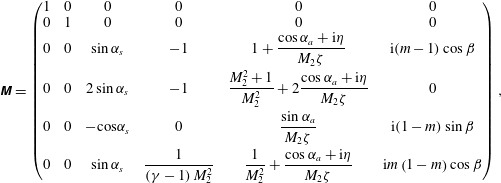 $$\begin{eqnarray}\displaystyle \unicode[STIX]{x1D648}=\left(\begin{array}{@{}cccccc@{}}1 & 0 & 0 & 0 & 0 & 0\\ 0 & 1 & 0 & 0 & 0 & 0\\ 0 & 0 & \sin \unicode[STIX]{x1D6FC}_{s} & -1 & 1+{\displaystyle \frac{\cos \unicode[STIX]{x1D6FC}_{a}+\text{i}\unicode[STIX]{x1D702}}{M_{2}\unicode[STIX]{x1D701}}} & \text{i}(m-1)\cos \unicode[STIX]{x1D6FD}\\ 0 & 0 & 2\sin \unicode[STIX]{x1D6FC}_{s} & -1 & {\displaystyle \frac{M_{2}^{2}+1}{M_{2}^{2}}}+2{\displaystyle \frac{\cos \unicode[STIX]{x1D6FC}_{a}+\text{i}\unicode[STIX]{x1D702}}{M_{2}\unicode[STIX]{x1D701}}} & 0\\ 0 & 0 & -\text{cos}\unicode[STIX]{x1D6FC}_{s} & 0 & {\displaystyle \frac{\sin \unicode[STIX]{x1D6FC}_{a}}{M_{2}\unicode[STIX]{x1D701}}} & \text{i}(1-m)\sin \unicode[STIX]{x1D6FD}\\ 0 & 0 & \sin \unicode[STIX]{x1D6FC}_{s} & {\displaystyle \frac{1}{\left(\unicode[STIX]{x1D6FE}-1\right)M_{2}^{2}}} & {\displaystyle \frac{1}{M_{2}^{2}}}+{\displaystyle \frac{\cos \unicode[STIX]{x1D6FC}_{a}+\text{i}\unicode[STIX]{x1D702}}{M_{2}\unicode[STIX]{x1D701}}} & \text{i}m\left(1-m\right)\cos \unicode[STIX]{x1D6FD}\end{array}\right), & & \displaystyle \nonumber\\ \displaystyle & & \displaystyle\end{eqnarray}$$
and the right-hand term, dependent on the incident wave’s nature,
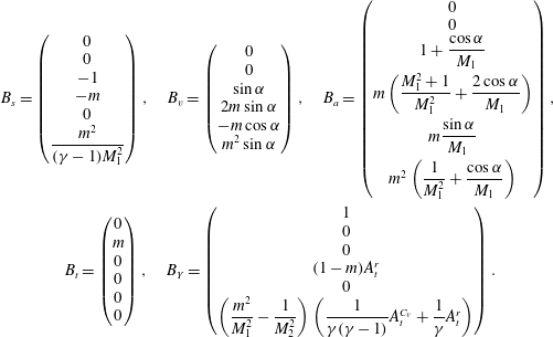 $$\begin{eqnarray}\displaystyle & \displaystyle B_{s}=\left(\begin{array}{@{}c@{}}0\\ 0\\ -1\\ -m\\ 0\\ {\displaystyle \frac{m^{2}}{(\unicode[STIX]{x1D6FE}-1)M_{1}^{2}}}\end{array}\right),\quad B_{v}=\left(\begin{array}{@{}c@{}}0\\ 0\\ \sin \unicode[STIX]{x1D6FC}\\ 2m\sin \unicode[STIX]{x1D6FC}\\ -m\cos \unicode[STIX]{x1D6FC}\\ m^{2}\sin \unicode[STIX]{x1D6FC}\end{array}\right),\quad B_{a}=\left(\begin{array}{@{}c@{}}0\\ 0\\ 1+{\displaystyle \frac{\cos \unicode[STIX]{x1D6FC}}{M_{1}}}\\ m\left({\displaystyle \frac{M_{1}^{2}+1}{M_{1}^{2}}}+{\displaystyle \frac{2\cos \unicode[STIX]{x1D6FC}}{M_{1}}}\right)\\ m{\displaystyle \frac{\sin \unicode[STIX]{x1D6FC}}{M_{1}}}\\ m^{2}\left({\displaystyle \frac{1}{M_{1}^{2}}}+{\displaystyle \frac{\cos \unicode[STIX]{x1D6FC}}{M_{1}}}\right)\end{array}\right), & \displaystyle \nonumber\\ \displaystyle & \displaystyle B_{t}=\left(\begin{array}{@{}c@{}}0\\ m\\ 0\\ 0\\ 0\\ 0\end{array}\right),\quad B_{Y}=\left(\begin{array}{@{}c@{}}1\\ 0\\ 0\\ (1-m)A_{t}^{r}\\ 0\\ \left({\displaystyle \frac{m^{2}}{M_{1}^{2}}}-{\displaystyle \frac{1}{M_{2}^{2}}}\right)\left({\displaystyle \frac{1}{\unicode[STIX]{x1D6FE}(\unicode[STIX]{x1D6FE}-1)}}A_{t}^{C_{v}}+{\displaystyle \frac{1}{\unicode[STIX]{x1D6FE}}}A_{t}^{r}\right)\end{array}\right). & \displaystyle\end{eqnarray}$$
From the above system, the transfer function vector can be deduced as
 $$\begin{eqnarray}\left(Z_{iY},Z_{it},Z_{iv},Z_{is},Z_{ia},Z_{ix}\right)^{\text{T}}=M^{-1}B_{i},\end{eqnarray}$$
where the inverse matrix is a block diagonal matrix of the same form as
 $M$
. It can then be inferred that the toroidal mode is fully decoupled from the others
$M$
. It can then be inferred that the toroidal mode is fully decoupled from the others
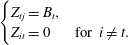 $$\begin{eqnarray}\left\{\begin{array}{@{}ll@{}}Z_{tj}=B_{t},\quad \\ Z_{it}=0\quad & \text{for }i\neq t.\end{array}\right.\end{eqnarray}$$
A similar behaviour is obtained for the concentration mode
 $Y$
, when
$Y$
, when
 $(A_{t}^{r},A_{t}^{C_{v}})=(0,0)$
and
$(A_{t}^{r},A_{t}^{C_{v}})=(0,0)$
and
 $B_{Y}$
comprises of a single non-zero component. For arbitrary values of
$B_{Y}$
comprises of a single non-zero component. For arbitrary values of
 $(A_{t}^{r},A_{t}^{C_{v}})$
, however,
$(A_{t}^{r},A_{t}^{C_{v}})$
, however,
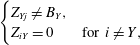 $$\begin{eqnarray}\left\{\begin{array}{@{}ll@{}}Z_{Yj}\neq B_{Y},\quad \\ Z_{iY}=0\quad & \text{for }i\neq Y,\end{array}\right.\end{eqnarray}$$
so that an upstream mass concentration perturbation can produce a combination of various modes downstream of the shock. Downstream, however, a mass fraction perturbation can only arise from an upstream mass fraction perturbation. These comments allow us to consider a reduced number of
 $Z_{ij}$
terms in the following figures.
$Z_{ij}$
terms in the following figures.
The transfer functions obtained for acoustic, poloidal and entropy incident perturbations are plotted in figure 5 as functions of the incident angle
 $\unicode[STIX]{x1D6FC}$
. The associated emitted wave vectors are found in figure 4 (
$\unicode[STIX]{x1D6FC}$
. The associated emitted wave vectors are found in figure 4 (
 $\unicode[STIX]{x1D6FC}_{a}$
for
$\unicode[STIX]{x1D6FC}_{a}$
for
 $Z_{ai}$
and
$Z_{ai}$
and
 $\unicode[STIX]{x1D6FC}_{s}$
for
$\unicode[STIX]{x1D6FC}_{s}$
for
 $Z_{vi}$
and
$Z_{vi}$
and
 $Z_{si}$
).
$Z_{si}$
).
Figure 5. Real part (plain line) and imaginary part (dashed) of
 $Z_{ii}$
as a function of the incident wave angle
$Z_{ii}$
as a function of the incident wave angle
 $\unicode[STIX]{x1D6FC}$
, for
$\unicode[STIX]{x1D6FC}$
, for
 $\unicode[STIX]{x1D6FE}=1.4$
,
$\unicode[STIX]{x1D6FE}=1.4$
,
 $M_{1}=2$
and
$M_{1}=2$
and
 $q=-2.25$
. The corresponding emitted wave vectors angles
$q=-2.25$
. The corresponding emitted wave vectors angles
 $\unicode[STIX]{x1D6FC}_{a}$
and
$\unicode[STIX]{x1D6FC}_{a}$
and
 $\unicode[STIX]{x1D6FC}_{s}$
are those represented in figure 4.
$\unicode[STIX]{x1D6FC}_{s}$
are those represented in figure 4.
Incident mass fraction perturbations can vary in nature depending on the value of the Atwood number
 $(A_{t}^{r},A_{t}^{C_{v}})$
defined earlier (2.3). The associated transfer functions
$(A_{t}^{r},A_{t}^{C_{v}})$
defined earlier (2.3). The associated transfer functions
 $Z_{Yi}$
are therefore provided separately, in figure 6, with associated emitted wave angles
$Z_{Yi}$
are therefore provided separately, in figure 6, with associated emitted wave angles
 $\unicode[STIX]{x1D6FC}_{s}$
in figure 4. Note that
$\unicode[STIX]{x1D6FC}_{s}$
in figure 4. Note that
 $B_{Y}$
is linear in
$B_{Y}$
is linear in
 $A_{t}^{r}$
and
$A_{t}^{r}$
and
 $A_{t}^{C_{v}}$
, so that providing solutions
$A_{t}^{C_{v}}$
, so that providing solutions
 $Z_{Yi}$
for the two base vectors
$Z_{Yi}$
for the two base vectors
 $(A_{t}^{r},A_{t}^{C_{v}})=(0,1)$
and
$(A_{t}^{r},A_{t}^{C_{v}})=(0,1)$
and
 $(A_{t}^{r},A_{t}^{C_{v}})=(1,0)$
suffices to describe the transfer function for any
$(A_{t}^{r},A_{t}^{C_{v}})=(1,0)$
suffices to describe the transfer function for any
 $(A_{t}^{r},A_{t}^{C_{v}})$
.
$(A_{t}^{r},A_{t}^{C_{v}})$
.
Figure 6. Real part (plain line) and imaginary part (dashed) of
 $Z_{Yi}$
as a function of the incident wave angle
$Z_{Yi}$
as a function of the incident wave angle
 $\unicode[STIX]{x1D6FC}$
, for different incident mass fraction waves:
$\unicode[STIX]{x1D6FC}$
, for different incident mass fraction waves:
 $(A_{t}^{r},A_{t}^{C_{v}})=$
(1, 0) (a–d), (0, 1) (e–h). The remaining parameters are identical to figure 5:
$(A_{t}^{r},A_{t}^{C_{v}})=$
(1, 0) (a–d), (0, 1) (e–h). The remaining parameters are identical to figure 5:
 $\unicode[STIX]{x1D6FE}=1.4$
,
$\unicode[STIX]{x1D6FE}=1.4$
,
 $M_{1}=2$
and
$M_{1}=2$
and
 $q=-2.25$
. The corresponding emitted wave vector angle
$q=-2.25$
. The corresponding emitted wave vector angle
 $\unicode[STIX]{x1D6FC}_{s}$
can be found in figure 4.
$\unicode[STIX]{x1D6FC}_{s}$
can be found in figure 4.
6 Interaction with Gaussian spots
This section is dedicated to the interaction between 2-D Gaussian spots advected at the uniform speed
 $U_{1}$
in the shock-normal direction and a planar shock wave.
$U_{1}$
in the shock-normal direction and a planar shock wave.
The Gaussian spots are introduced as perturbations of the form
 $$\begin{eqnarray}\displaystyle G^{\prime }=\unicode[STIX]{x1D716}\text{e}^{-r^{2}}, & & \displaystyle\end{eqnarray}$$
where
 $r$
is the radial coordinate relative to the centre of the spot, and the Gaussian perturbation
$r$
is the radial coordinate relative to the centre of the spot, and the Gaussian perturbation
 $G^{\prime }$
is successively set as three elemental perturbations
$G^{\prime }$
is successively set as three elemental perturbations
 $$\begin{eqnarray}\left\{\begin{array}{@{}ll@{}}G^{\prime }={\displaystyle \frac{\unicode[STIX]{x1D70F}^{\prime }}{A_{t}^{r}\,\unicode[STIX]{x1D70F}}}\quad & \text{for the density spot,}\\ G^{\prime }={\displaystyle \frac{s^{\prime }}{c_{p}}}\quad & \text{for the entropy spot,}\\ G^{\prime }={\displaystyle \frac{\unicode[STIX]{x1D714}^{\prime }}{U}}\quad & \text{for the vorticity spot.}\end{array}\right.\end{eqnarray}$$
For each perturbation, the emitted flow will systematically be studied through comparisons of acoustic, entropy and vorticity fields.
Note that, owing to the linear character of this study, it is straightforward to combine these three elemental Gaussian perturbations into more complex ones, and obtain the emitted flow field. This is illustrated in figure 7, which displays the vorticity field emitted from the combination of the three elemental spots presented hereafter.
In the following
 $\unicode[STIX]{x1D716}$
, appears as a mere scaling and is therefore set to 1. Typical results are shown for
$\unicode[STIX]{x1D716}$
, appears as a mere scaling and is therefore set to 1. Typical results are shown for
 $A_{t}^{r}=2$
,
$A_{t}^{r}=2$
,
 $A_{t}^{C_{v}}=1$
,
$A_{t}^{C_{v}}=1$
,
 $M_{1}=2$
and
$M_{1}=2$
and
 $\unicode[STIX]{x1D6FE}=1.4$
. To illustrate the effect of the heat release, results are plotted for adiabatic (
$\unicode[STIX]{x1D6FE}=1.4$
. To illustrate the effect of the heat release, results are plotted for adiabatic (
 $q=0$
), endothermic (
$q=0$
), endothermic (
 $q=-2.25$
) and exothermic (
$q=-2.25$
) and exothermic (
 $q=0.59$
) cases. The numeric values for endothermic and exothermic shocks were chosen to be
$q=0.59$
) cases. The numeric values for endothermic and exothermic shocks were chosen to be
 $q_{min}/2$
and
$q_{min}/2$
and
 $q_{max}/2$
at
$q_{max}/2$
at
 $M_{1}=2$
.
$M_{1}=2$
.
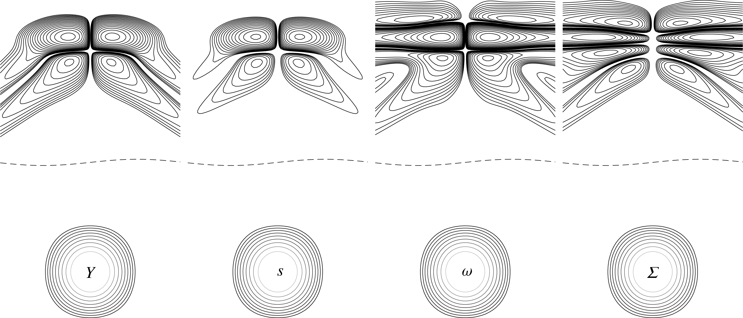
Figure 7. Emitted vorticity for incident Gaussian density
 $Y$
, entropy
$Y$
, entropy
 $s$
and vorticity
$s$
and vorticity
 $\unicode[STIX]{x1D714}$
spots. The fourth spot corresponds to the sum
$\unicode[STIX]{x1D714}$
spots. The fourth spot corresponds to the sum
 $\unicode[STIX]{x1D6F4}$
of the three Gaussian spots, resulting in yet another vorticity pattern. The dashed line illustrates the corrugated shock.
$\unicode[STIX]{x1D6F4}$
of the three Gaussian spots, resulting in yet another vorticity pattern. The dashed line illustrates the corrugated shock.
6.1 Gaussian density spot
Let us now consider a density spot, e.g.
 $G^{\prime }=(\unicode[STIX]{x1D70F}^{\prime }/A_{t}^{r}\,\unicode[STIX]{x1D70F})$
in (6.2), which can be considered as an idealized model for shock/droplet interaction.
$G^{\prime }=(\unicode[STIX]{x1D70F}^{\prime }/A_{t}^{r}\,\unicode[STIX]{x1D70F})$
in (6.2), which can be considered as an idealized model for shock/droplet interaction.
The choice of a positive
 $\unicode[STIX]{x1D716}$
in (6.2) corresponds to the definition of a heavy perturbation with respect to the upstream fluid, which can be interpreted as an ideal model for a droplet of heavy fluid. A negative value would correspond a pocket of light fluid. It is worth noting that pure density heterogeneities without acoustic perturbation, i.e. pure
$\unicode[STIX]{x1D716}$
in (6.2) corresponds to the definition of a heavy perturbation with respect to the upstream fluid, which can be interpreted as an ideal model for a droplet of heavy fluid. A negative value would correspond a pocket of light fluid. It is worth noting that pure density heterogeneities without acoustic perturbation, i.e. pure
 $\unicode[STIX]{x1D70C}$
-waves, are obtained considering concentration fluctuations. The solution is then computed analytically thanks to the formulas given in appendix A.
$\unicode[STIX]{x1D70C}$
-waves, are obtained considering concentration fluctuations. The solution is then computed analytically thanks to the formulas given in appendix A.
The emitted fields of normalized entropy
 $s^{\prime }/C_{p}$
and vorticity
$s^{\prime }/C_{p}$
and vorticity
 $a\unicode[STIX]{x1D714}^{\prime }/\bar{u}$
are displayed in the first 4 plots of figure 8. Since the emitted patterns are advected at the constant speed
$a\unicode[STIX]{x1D714}^{\prime }/\bar{u}$
are displayed in the first 4 plots of figure 8. Since the emitted patterns are advected at the constant speed
 $U_{2}$
, they are plotted in the reference frame associated with the perturbation centre, in which they are frozen thanks to the fact that diffusive effects are not taken into account in the present inviscid model. The presented patterns are related to the far field solution, i.e. intermediary solutions that are found at times at which the incoming fluctuation spot has not totally crossed the shock are not presented for the sake of brevity (but can be computed).
$U_{2}$
, they are plotted in the reference frame associated with the perturbation centre, in which they are frozen thanks to the fact that diffusive effects are not taken into account in the present inviscid model. The presented patterns are related to the far field solution, i.e. intermediary solutions that are found at times at which the incoming fluctuation spot has not totally crossed the shock are not presented for the sake of brevity (but can be computed).

Figure 8. Incident Gaussian density spot: emitted entropy, vorticity and acoustic perturbations (from a to f). (a,c,e) Adiabatic versus endothermic case. (b,d,f) Adiabatic versus exothermic.
It is seen that the topology of the emitted vorticity field is qualitatively the same in the three cases: a quadripolar pattern made of two counter-rotating vortex pairs is generated. This can be qualitatively interpreted as the result of a baroclinic effect of the form
 $-(\unicode[STIX]{x1D735}p\times \unicode[STIX]{x1D735}\unicode[STIX]{x1D70C})/\unicode[STIX]{x1D70C}^{2}$
, in which the positive pressure gradient is related to the pressure jump across the shock wave. From that expression, it is seen that the case of a light disturbance with a negative amplitude parameter
$-(\unicode[STIX]{x1D735}p\times \unicode[STIX]{x1D735}\unicode[STIX]{x1D70C})/\unicode[STIX]{x1D70C}^{2}$
, in which the positive pressure gradient is related to the pressure jump across the shock wave. From that expression, it is seen that the case of a light disturbance with a negative amplitude parameter
 $\unicode[STIX]{x1D716}$
would lead to a vorticity pattern with opposite sign, i.e. a pattern made of four vortices rotating in the opposite sense to those found for a heavy density spot.
$\unicode[STIX]{x1D716}$
would lead to a vorticity pattern with opposite sign, i.e. a pattern made of four vortices rotating in the opposite sense to those found for a heavy density spot.
The main effects of the heat source term being (i) an amplification (respectively damping) of the amplitude of the emitted perturbations and (ii) an increase (respectively decrease) of the anisotropy of the emitted pattern for endothermic (respectively exothermic) case, when compared to the adiabatic case. In the strong endothermic case the amplitude of the four vortices are nearly equal, while the second vortex pair is weaker in other cases. This is consistent with the fact that the effective shock-induced compressive effect is stronger in the endothermic case, as observed in § 2.
The emitted acoustic field is illustrated here in the bottom plots of figure 8, in which the acoustic pressure field
 $p^{\prime }/\unicode[STIX]{x1D6FE}\bar{p}$
is plotted at time
$p^{\prime }/\unicode[STIX]{x1D6FE}\bar{p}$
is plotted at time
 $t=(4a/c_{2})$
.
$t=(4a/c_{2})$
.
A more global view at the interaction physics is obtained looking at the energy of the emitted waves along with the part associated with each Kovásznay mode, according to the extended definition derived in § 4. The area used to compute the sum in (4.13) is taken equal to
 $12D\,\times \,12D$
, which was checked to be large enough to get fully converged values, with
$12D\,\times \,12D$
, which was checked to be large enough to get fully converged values, with
 $D$
defined as the radius of the incident Gaussian spot (see appendix A).
$D$
defined as the radius of the incident Gaussian spot (see appendix A).
Results in the
 $(M_{1},q)$
plane normalized by the energy of the incident density spot are displayed in figure 9 for the far-field solution, i.e. the transient contribution of acoustic non-propagative waves is omitted. Profiles along the
$(M_{1},q)$
plane normalized by the energy of the incident density spot are displayed in figure 9 for the far-field solution, i.e. the transient contribution of acoustic non-propagative waves is omitted. Profiles along the
 $q=0$
and the
$q=0$
and the
 $M_{1}=2$
lines are also shown in figure 10.
$M_{1}=2$
lines are also shown in figure 10.
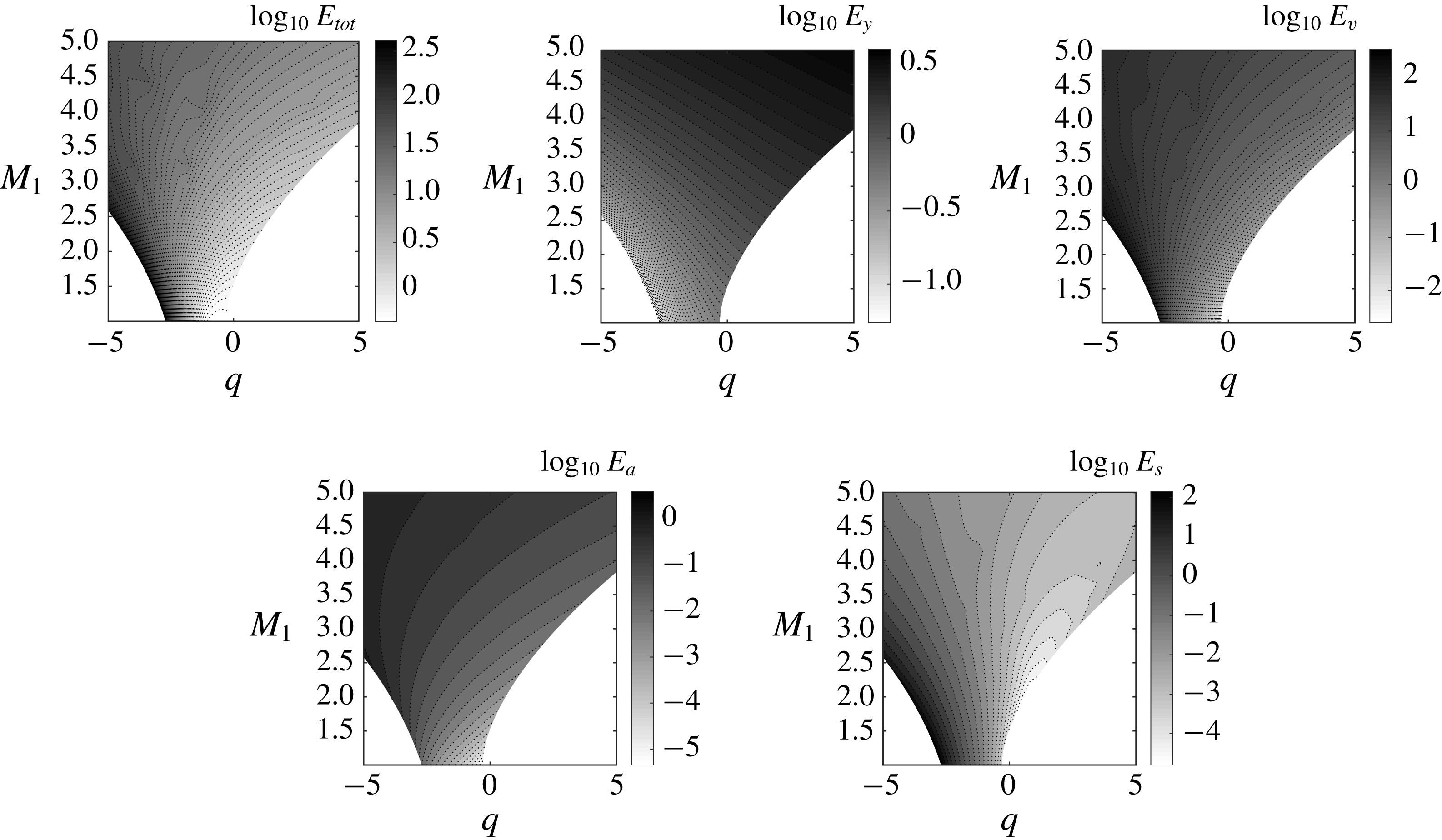
Figure 9. Energy of the emitted disturbances in the case of an incident Gaussian density spot in the
 $(M_{1},q)$
plane. Total energy
$(M_{1},q)$
plane. Total energy
 $E_{tot}$
and the part associated with each Kovásznay mode are displayed, with
$E_{tot}$
and the part associated with each Kovásznay mode are displayed, with
 $E_{y}$
: energy of the concentration mode;
$E_{y}$
: energy of the concentration mode;
 $E_{v}$
: energy of the vorticity mode;
$E_{v}$
: energy of the vorticity mode;
 $E_{a}$
: energy of the acoustic mode;
$E_{a}$
: energy of the acoustic mode;
 $E_{s}$
: energy of the entropy mode.
$E_{s}$
: energy of the entropy mode.
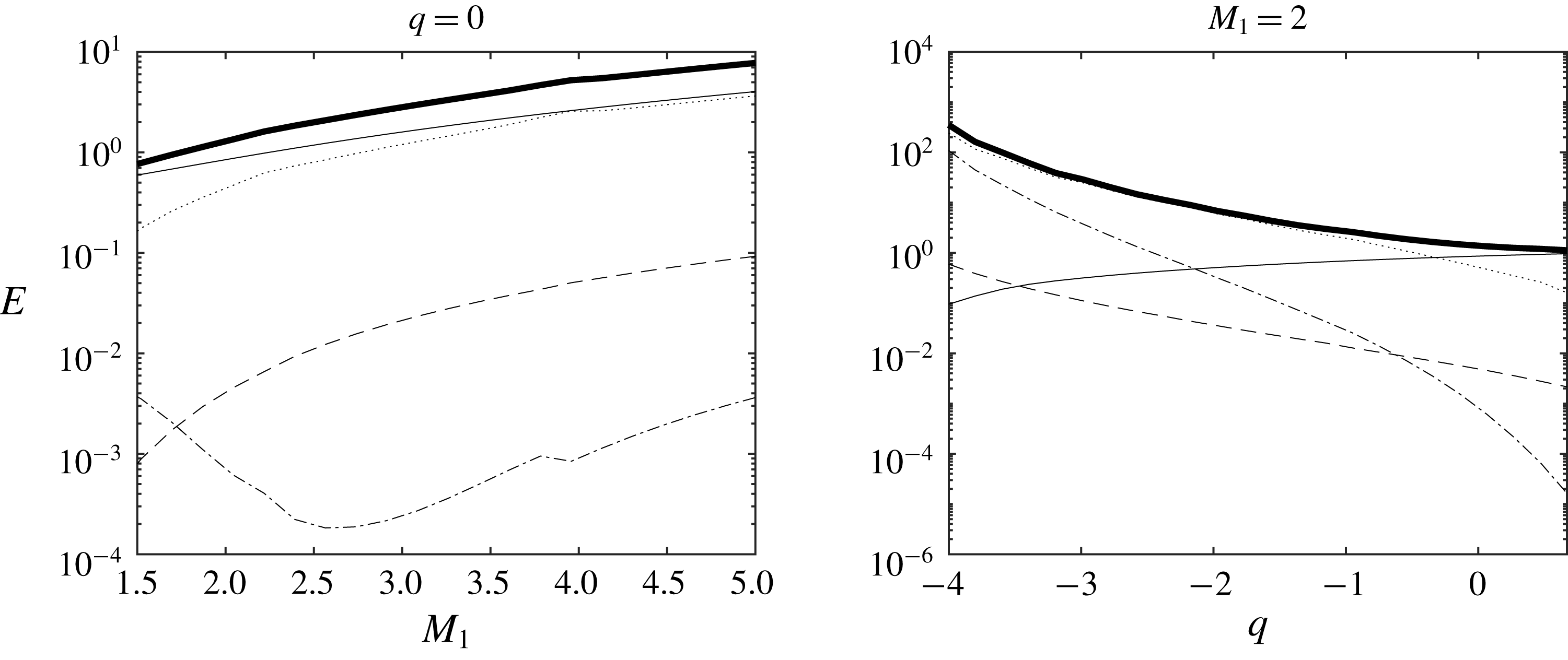
Figure 10. Energy of the emitted disturbances in the case of an incident Gaussian density spot versus
 $M_{1}$
for the adiabatic case (
$M_{1}$
for the adiabatic case (
 $q=0$
) and versus
$q=0$
) and versus
 $q$
for
$q$
for
 $M_{1}=2$
. Total energy and the part associated with each Kovásznay mode are displayed.
$M_{1}=2$
. Total energy and the part associated with each Kovásznay mode are displayed.
 $E_{tot}$
(solid thick line),
$E_{tot}$
(solid thick line),
 $E_{y}$
(solid),
$E_{y}$
(solid),
 $E_{v}$
(dotted),
$E_{v}$
(dotted),
 $E_{a}$
(dashed),
$E_{a}$
(dashed),
 $E_{s}$
(dotted-dashed).
$E_{s}$
(dotted-dashed).
It is observed that the total emitted energy is an increasing function of the incoming Mach number
 $M_{1}$
, and that the respective importance of each mode is strongly influenced by the heat source term
$M_{1}$
, and that the respective importance of each mode is strongly influenced by the heat source term
 $q$
. In the neutral case
$q$
. In the neutral case
 $q=0$
, the emitted energy is mainly due
$q=0$
, the emitted energy is mainly due
 $E_{y}$
and
$E_{y}$
and
 $E_{v}$
, i.e. to the concentration mode and the vorticity mode, the former being dominant for
$E_{v}$
, i.e. to the concentration mode and the vorticity mode, the former being dominant for
 $M_{1}<4$
. It is worth noting that the energy of all emitted modes is an increasing function of
$M_{1}<4$
. It is worth noting that the energy of all emitted modes is an increasing function of
 $M_{1}$
, excepting
$M_{1}$
, excepting
 $E_{s}$
, which decreases for
$E_{s}$
, which decreases for
 $1\leqslant M_{1}\leqslant 2.6$
. Varying
$1\leqslant M_{1}\leqslant 2.6$
. Varying
 $q$
at fixed
$q$
at fixed
 $M_{1}$
makes a more complex behaviour appears. The emitted energy is mostly related to the vorticity mode in the endothermic case, the solution being dominated by the concentration mode for slightly negative
$M_{1}$
makes a more complex behaviour appears. The emitted energy is mostly related to the vorticity mode in the endothermic case, the solution being dominated by the concentration mode for slightly negative
 $q$
and exothermic cases. This is due to the case that the concentration mode is the only one which exhibits an increase for increasing
$q$
and exothermic cases. This is due to the case that the concentration mode is the only one which exhibits an increase for increasing
 $q$
, while a decrease of the total emitted energy
$q$
, while a decrease of the total emitted energy
 $E_{tot}$
associated with a monotonic decrease of all other modes is observed. A very fast decrease of
$E_{tot}$
associated with a monotonic decrease of all other modes is observed. A very fast decrease of
 $E_{s}$
is observed, leading to the fact that the entropy mode is very strong in the highly endothermic case, while it is the weakest mode in the neutral and exothermic cases.
$E_{s}$
is observed, leading to the fact that the entropy mode is very strong in the highly endothermic case, while it is the weakest mode in the neutral and exothermic cases.
6.2 Gaussian entropy spot
This section is dedicated to the interaction with a Gaussian entropy spot, and therefore is an extension of the previous analysis provided in Fabre et al. (Reference Fabre, Jacquin and Sesterhenn2001) for the adiabatic case
 $q=0$
. The upstream entropy spot is defined by setting
$q=0$
. The upstream entropy spot is defined by setting
 $G^{\prime }=(s^{\prime }/c_{p})$
in (6.2).
$G^{\prime }=(s^{\prime }/c_{p})$
in (6.2).
The emitted entropy far field, vorticity far field and acoustic pressure far field are displayed in figure 11. The emitted disturbance topology is the same as in the density case: a quadrupolar pattern made of two counter-rotating vortex pairs is generated downstream the shock, whose intensity and anisotropy are decreasing functions of the heat source term
 $q$
. The key mechanisms for vorticity generation can again be interpreted as a kind of baroclinic production term associated with the pressure jump across the shock and the density gradient associated with the entropy disturbance, see (3.5).
$q$
. The key mechanisms for vorticity generation can again be interpreted as a kind of baroclinic production term associated with the pressure jump across the shock and the density gradient associated with the entropy disturbance, see (3.5).
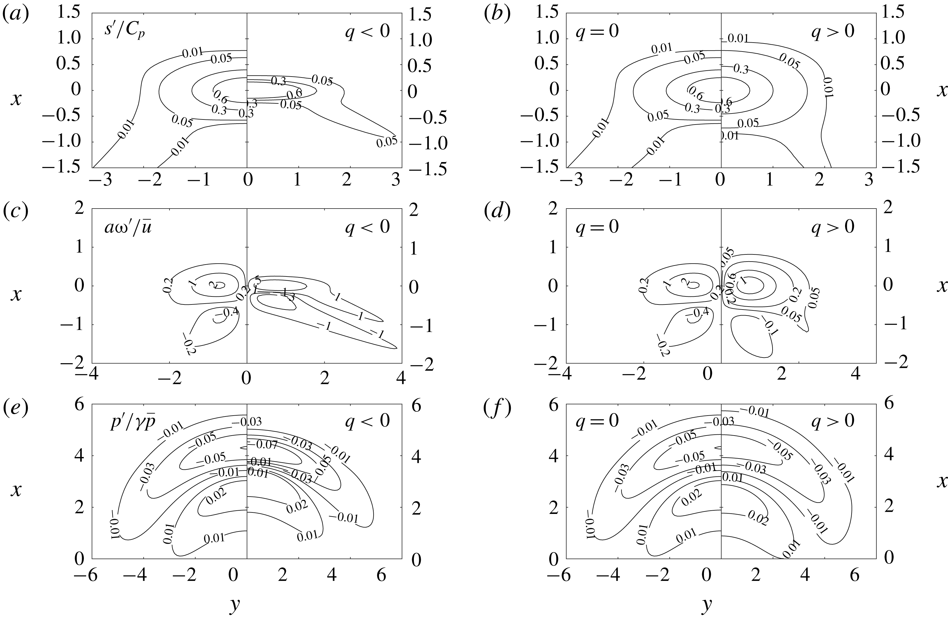
Figure 11. Incident Gaussian entropy spot: emitted entropy, vorticity and acoustic perturbations (from a to f). (a,c,e) Adiabatic versus endothermic case. (b,d,f) Adiabatic versus exothermic.
The total energy of the emitted far-field solution (normalized by the energy of the incident spot) and the part associated with each Kovásznay component are plotted in figure 12 in the
 $(M_{1},q)$
plane, while profiles along the
$(M_{1},q)$
plane, while profiles along the
 $M_{1}=2$
and
$M_{1}=2$
and
 $q=0$
lines are shown in figure 13. It is worth noting that the concentration mode energy remains null downstream of the shock, i.e.
$q=0$
lines are shown in figure 13. It is worth noting that the concentration mode energy remains null downstream of the shock, i.e.
 $E_{y}=0$
, since it is null upstream of the shock and the concentration fluctuation is continuous at the shock according to (5.1).
$E_{y}=0$
, since it is null upstream of the shock and the concentration fluctuation is continuous at the shock according to (5.1).
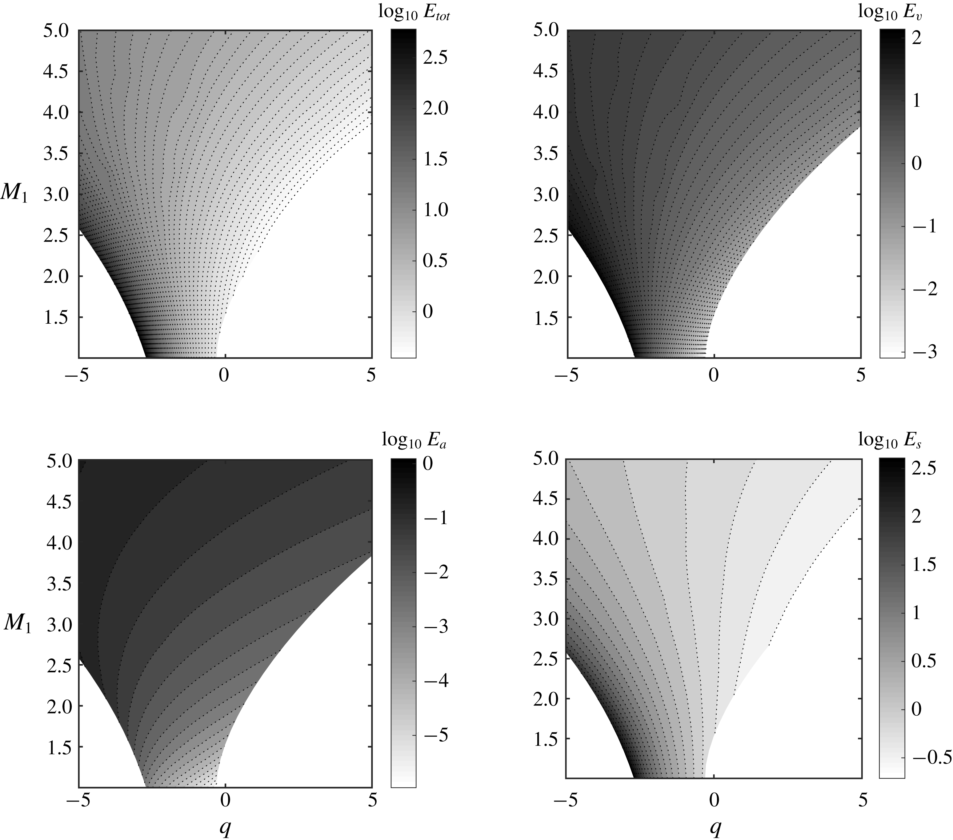
Figure 12. Energy of the emitted disturbances in the case of an incident Gaussian entropy spot in the
 $(M_{1},q)$
plane. Total energy
$(M_{1},q)$
plane. Total energy
 $E_{tot}$
and the part associated with each Kovásznay mode are displayed, with
$E_{tot}$
and the part associated with each Kovásznay mode are displayed, with
 $E_{v}$
: energy of the vorticity mode;
$E_{v}$
: energy of the vorticity mode;
 $E_{a}$
: energy of the acoustic mode;
$E_{a}$
: energy of the acoustic mode;
 $E_{s}$
: energy of the entropy mode.
$E_{s}$
: energy of the entropy mode.
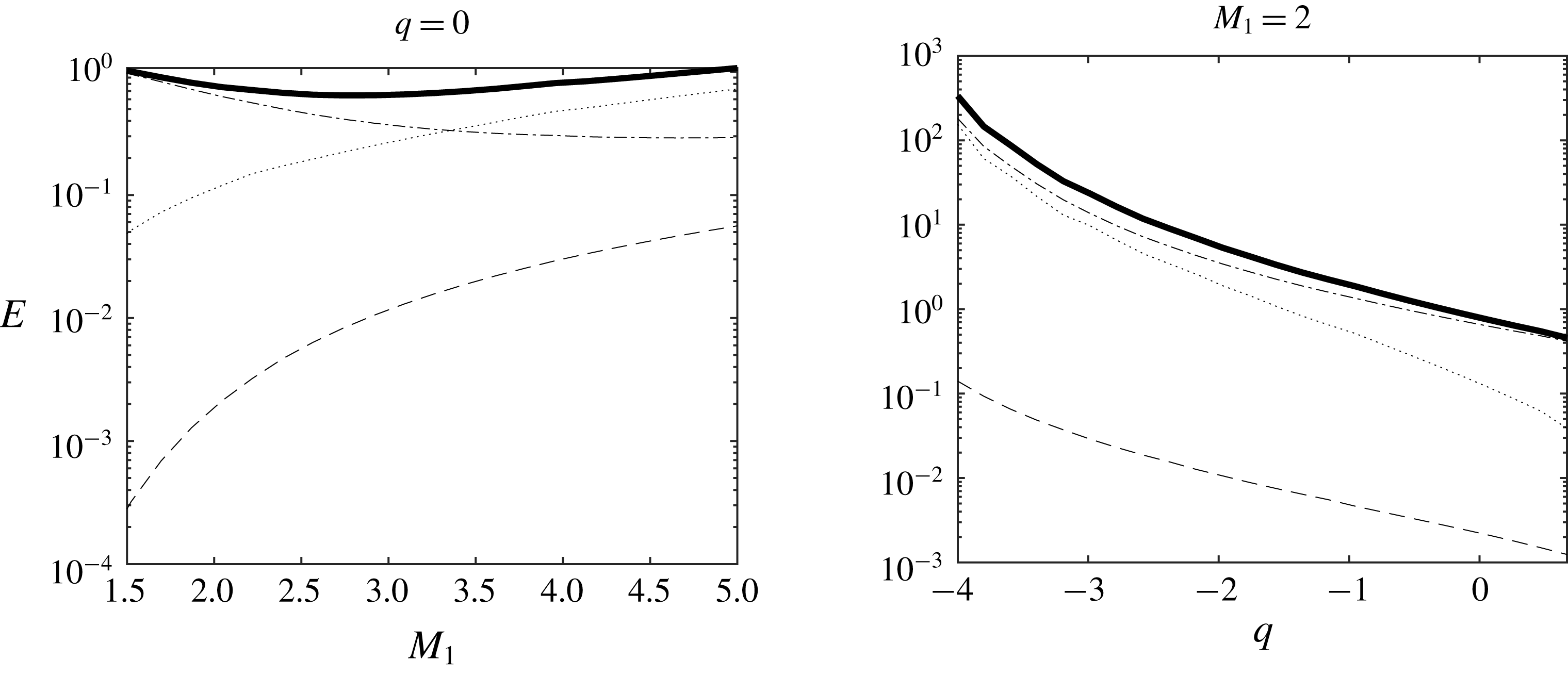
Figure 13. Energy of the emitted disturbances in the case of an incident Gaussian entropy spot versus
 $M_{1}$
for in the adiabatic case (
$M_{1}$
for in the adiabatic case (
 $q=0$
) (top) and versus
$q=0$
) (top) and versus
 $q$
for
$q$
for
 $M_{1}=2$
(bottom). Total energy and the part associated with each Kovásznay mode are displayed.
$M_{1}=2$
(bottom). Total energy and the part associated with each Kovásznay mode are displayed.
 $E_{tot}$
(solid thick line),
$E_{tot}$
(solid thick line),
 $E_{v}$
(dotted),
$E_{v}$
(dotted),
 $E_{a}$
(dashed),
$E_{a}$
(dashed),
 $E_{s}$
(dotted-dashed).
$E_{s}$
(dotted-dashed).
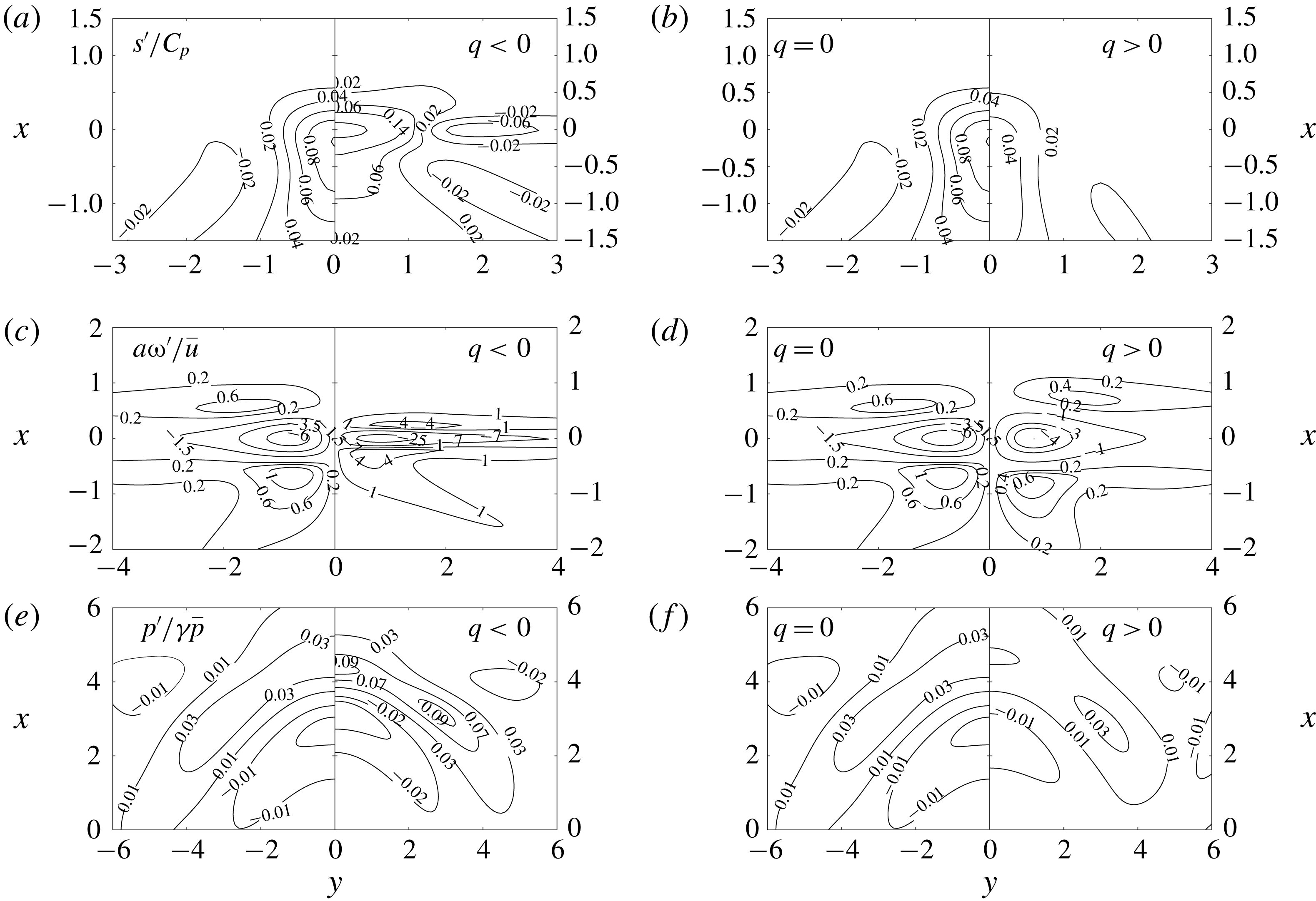
Figure 14. Incident weak vortex/Gaussian vorticity spot: emitted entropy, vorticity and acoustic perturbations (from a to f). (a,c,e) Adiabatic versus endothermic case. (b,d,f) Adiabatic versus exothermic.
Some interesting differences with the density spot case are observed, which are due to the fact that the entropy spot combines a density disturbance and a temperature disturbance. First, in the adiabatic case
 $q=0$
, the normalized total emitted energy is not a monotonic function of the upstream Mach number
$q=0$
, the normalized total emitted energy is not a monotonic function of the upstream Mach number
 $M_{1}$
. A decrease is observed for
$M_{1}$
. A decrease is observed for
 $M_{1}<M_{crit}\simeq 2.7$
, which is due to a decrease of the energy of the emitted entropy mode, which is a monotonically decaying function of
$M_{1}<M_{crit}\simeq 2.7$
, which is due to a decrease of the energy of the emitted entropy mode, which is a monotonically decaying function of
 $M_{1}$
. The emitted acoustic and vorticity energy components,
$M_{1}$
. The emitted acoustic and vorticity energy components,
 $E_{a}$
and
$E_{a}$
and
 $E_{v}$
, are growing with
$E_{v}$
, are growing with
 $M_{1}$
,
$M_{1}$
,
 $E_{a}$
being negligible in all cases. Therefore, the emitted field is dominated by the entropy mode for
$E_{a}$
being negligible in all cases. Therefore, the emitted field is dominated by the entropy mode for
 $M_{1}<M_{crit}$
, while the vorticity mode is dominant at higher Mach number. This picture is very different from the one observed for the density spot, and it is stable with respect to a change in the parameter
$M_{1}<M_{crit}$
, while the vorticity mode is dominant at higher Mach number. This picture is very different from the one observed for the density spot, and it is stable with respect to a change in the parameter
 $q$
. Here, the energy of all emitted modes decays when increasing
$q$
. Here, the energy of all emitted modes decays when increasing
 $q$
, including the emitted vortical energy which was an increasing function of
$q$
, including the emitted vortical energy which was an increasing function of
 $q$
in the density spot case.
$q$
in the density spot case.
6.3 Gaussian vorticity spot
The last case deals with the interaction between a planar shock wave and a Gaussian vorticity spot, which is a model of a weak vortex. The shock/vortex interaction has been addressed by several authors, mainly via DNS, but the present analysis is the first one to cover the full
 $(M_{1},q)$
plane within the LIA framework.
$(M_{1},q)$
plane within the LIA framework.
Results for the emitted non-acoustic fields are shown in the first 4 plots of figure 14. The concentration field remains uniform, as in the case of the entropy spot. A first observation is that the topology of the emitted field is different from the one observed for both incident density and entropy spot. As a matter of fact, while two vortex pairs with variable intensity were found previously, the present field is made of a strong counter-rotating vortex pair, with two companion pairs of much weaker vortical structures.
The topology of the downstream acoustic field is investigated in the bottom plots of figure 14 which displays the generated pressure. A compression wave followed by a dilatation wave is observed, while in the two other cases the dilatation wave is emitted first.
The energy of the emitted field split into model components, normalized by the energy of the incident spot, is displayed in figures 15 and 16. It is observed that, in all cases, the emitted energy is dominated by the vortical component. In the adiabatic case, the acoustic energy remains larger than the entropy mode energy at all Mach numbers. The opposite trend can be observed in strongly endothermic cases. All energy components are growing functions of
 $M_{1}$
and decreasing functions of
$M_{1}$
and decreasing functions of
 $q$
.
$q$
.
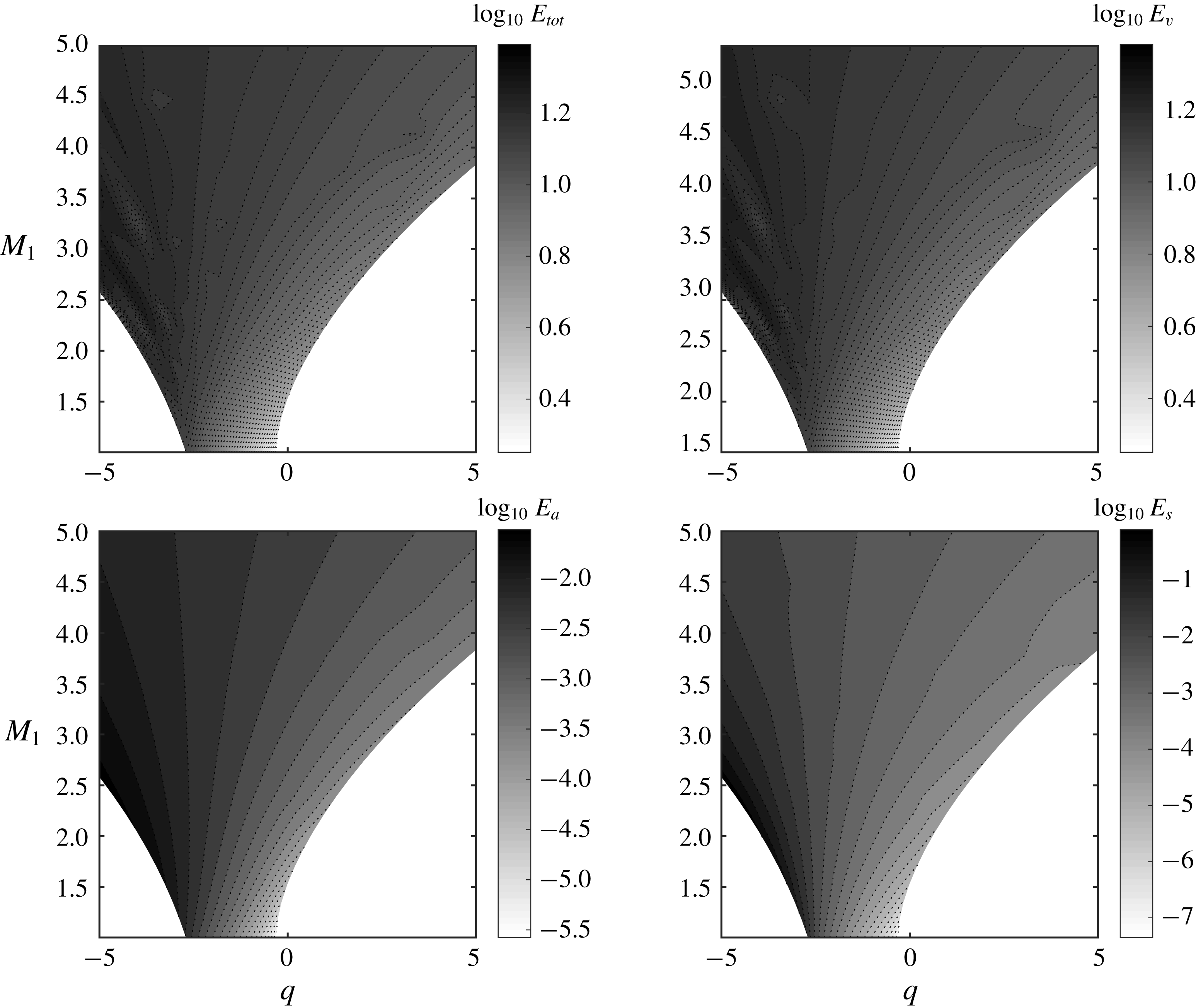
Figure 15. Energy of the emitted disturbances in the case of an incident weak vortex/Gaussian vorticity spot in the
 $(M_{1},q)$
plane. Total energy
$(M_{1},q)$
plane. Total energy
 $E_{tot}$
and the part associated with each Kovásznay mode are displayed, with
$E_{tot}$
and the part associated with each Kovásznay mode are displayed, with
 $E_{v}$
: energy of the vorticity mode;
$E_{v}$
: energy of the vorticity mode;
 $E_{a}$
: energy of the acoustic mode;
$E_{a}$
: energy of the acoustic mode;
 $E_{s}$
: energy of the entropy mode.
$E_{s}$
: energy of the entropy mode.
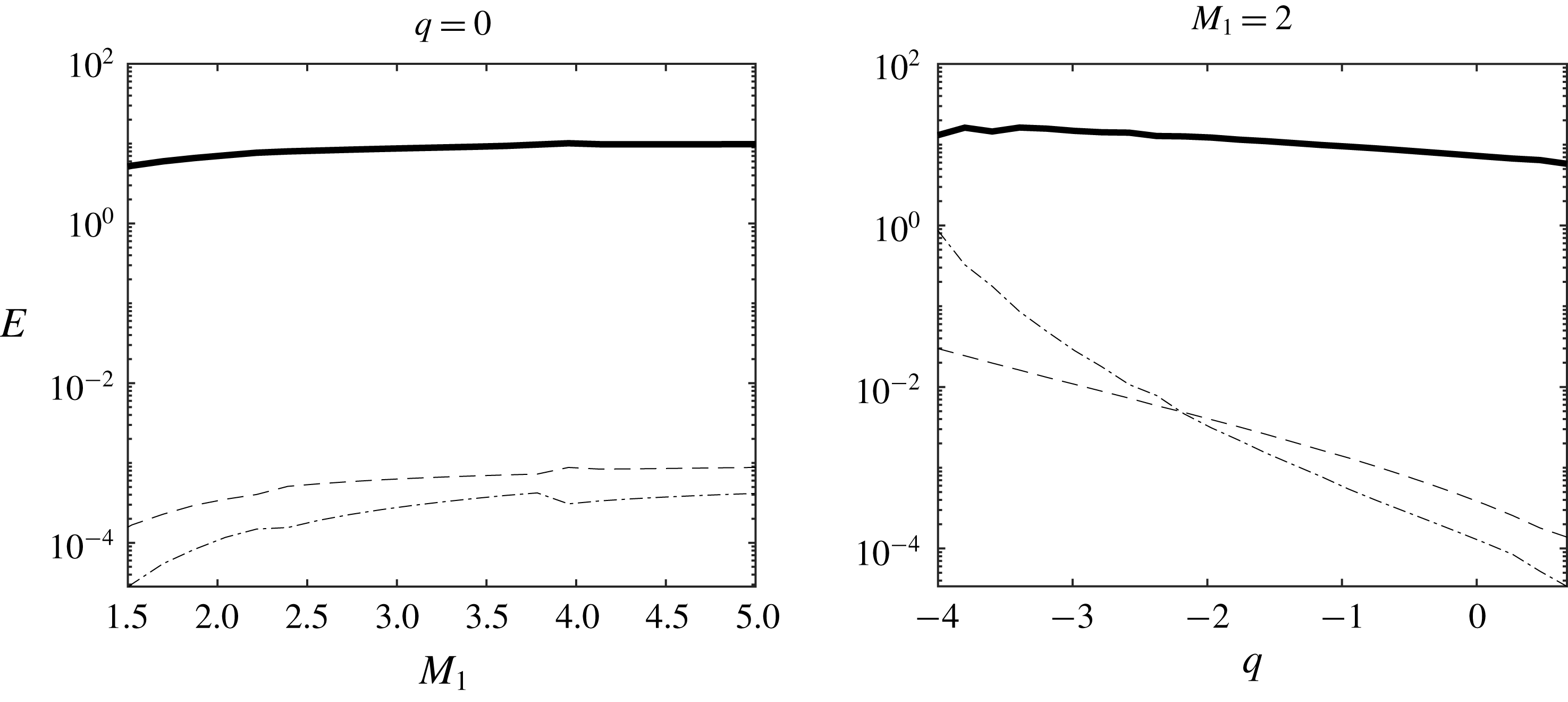
Figure 16. Energy of the emitted disturbances in the case of a weak vortex/Gaussian vorticity spot versus
 $M_{1}$
for in the adiabatic case and versus
$M_{1}$
for in the adiabatic case and versus
 $q$
for
$q$
for
 $M_{1}=2$
. Total energy and the part associated with each Kovásznay mode are displayed.
$M_{1}=2$
. Total energy and the part associated with each Kovásznay mode are displayed.
 $E_{tot}$
(solid thick line),
$E_{tot}$
(solid thick line),
 $E_{v}$
(dotted),
$E_{v}$
(dotted),
 $E_{a}$
(dashed),
$E_{a}$
(dashed),
 $E_{s}$
(dotted-dashed).
$E_{s}$
(dotted-dashed).
6.4 Optimal mixed disturbances with minimal radiated noise
The purpose of this section is to illustrate the possibility of finding upstream disturbances associated with a peculiar emitted field. To this end, we have chosen to find the optimal combination of the three above elementary spots for minimal radiated noise.
Let us identify the emitted pressure perturbation as
 $p_{Y}^{\prime }$
,
$p_{Y}^{\prime }$
,
 $p_{s}^{\prime }$
and
$p_{s}^{\prime }$
and
 $p_{\unicode[STIX]{x1D714}}^{\prime }$
for the density, entropy and vorticity Gaussian elementary spots. Next, we introduce
$p_{\unicode[STIX]{x1D714}}^{\prime }$
for the density, entropy and vorticity Gaussian elementary spots. Next, we introduce
 $\unicode[STIX]{x1D6F1}$
, the radiated noise emitted through the shock as
$\unicode[STIX]{x1D6F1}$
, the radiated noise emitted through the shock as
 $$\begin{eqnarray}\unicode[STIX]{x1D6F1}(a_{s},a_{Y})=\iint _{V}\left(\frac{p_{\unicode[STIX]{x1D714}}^{\prime }+a_{s}p_{s}^{\prime }+a_{Y}p_{Y}^{\prime }}{\unicode[STIX]{x1D6FE}\bar{p}}\right)^{2}\,\text{d}x\,\text{d}y,\end{eqnarray}$$
where
 $V$
is the volume of fluid after the shock. This corresponds to the acoustic perturbation obtained through a combination of elementary spots, as illustrated in figure 7, with coefficients
$V$
is the volume of fluid after the shock. This corresponds to the acoustic perturbation obtained through a combination of elementary spots, as illustrated in figure 7, with coefficients
 $(a_{Y},a_{s},1)$
for the three elementary spots. These combinations can be interpreted as a family of low-density hot vortices.
$(a_{Y},a_{s},1)$
for the three elementary spots. These combinations can be interpreted as a family of low-density hot vortices.
Figure 17 presents the result of the minimization of
 $\unicode[STIX]{x1D6F1}$
(6.3). The top two plots show the normalized relative amplitudes
$\unicode[STIX]{x1D6F1}$
(6.3). The top two plots show the normalized relative amplitudes
 $$\begin{eqnarray}\unicode[STIX]{x1D6FC}_{Y}=\frac{-a_{Y}}{1-a_{Y}+a_{s}},\quad \unicode[STIX]{x1D6FC}_{s}=\frac{a_{s}}{1-a_{Y}+a_{s}},\quad \unicode[STIX]{x1D6FC}_{\unicode[STIX]{x1D714}}=\frac{1}{1-a_{Y}+a_{s}},\end{eqnarray}$$
having found that
 $a_{Y}<0$
over the explored range of
$a_{Y}<0$
over the explored range of
 $(M_{1},q)$
. Note that the opposite sign found for
$(M_{1},q)$
. Note that the opposite sign found for
 $a_{s}$
and
$a_{s}$
and
 $a_{y}$
found to minimize
$a_{y}$
found to minimize
 $\unicode[STIX]{x1D6F1}$
could have been intuited from figures 8 and 11, the density and entropy spots leading to relatively similar emission patterns. The bottom two plots compare
$\unicode[STIX]{x1D6F1}$
could have been intuited from figures 8 and 11, the density and entropy spots leading to relatively similar emission patterns. The bottom two plots compare
 $\unicode[STIX]{x1D6F1}$
for the optimal
$\unicode[STIX]{x1D6F1}$
for the optimal
 $(a_{s},a_{y})$
with
$(a_{s},a_{y})$
with
 $\unicode[STIX]{x1D6F1}(0,0)$
, the noise radiated by the elementary Gaussian vorticity spot, showing that the vortex emitted noise was reduced by 80–90 % by superimposing the adequate density and entropy perturbations.
$\unicode[STIX]{x1D6F1}(0,0)$
, the noise radiated by the elementary Gaussian vorticity spot, showing that the vortex emitted noise was reduced by 80–90 % by superimposing the adequate density and entropy perturbations.
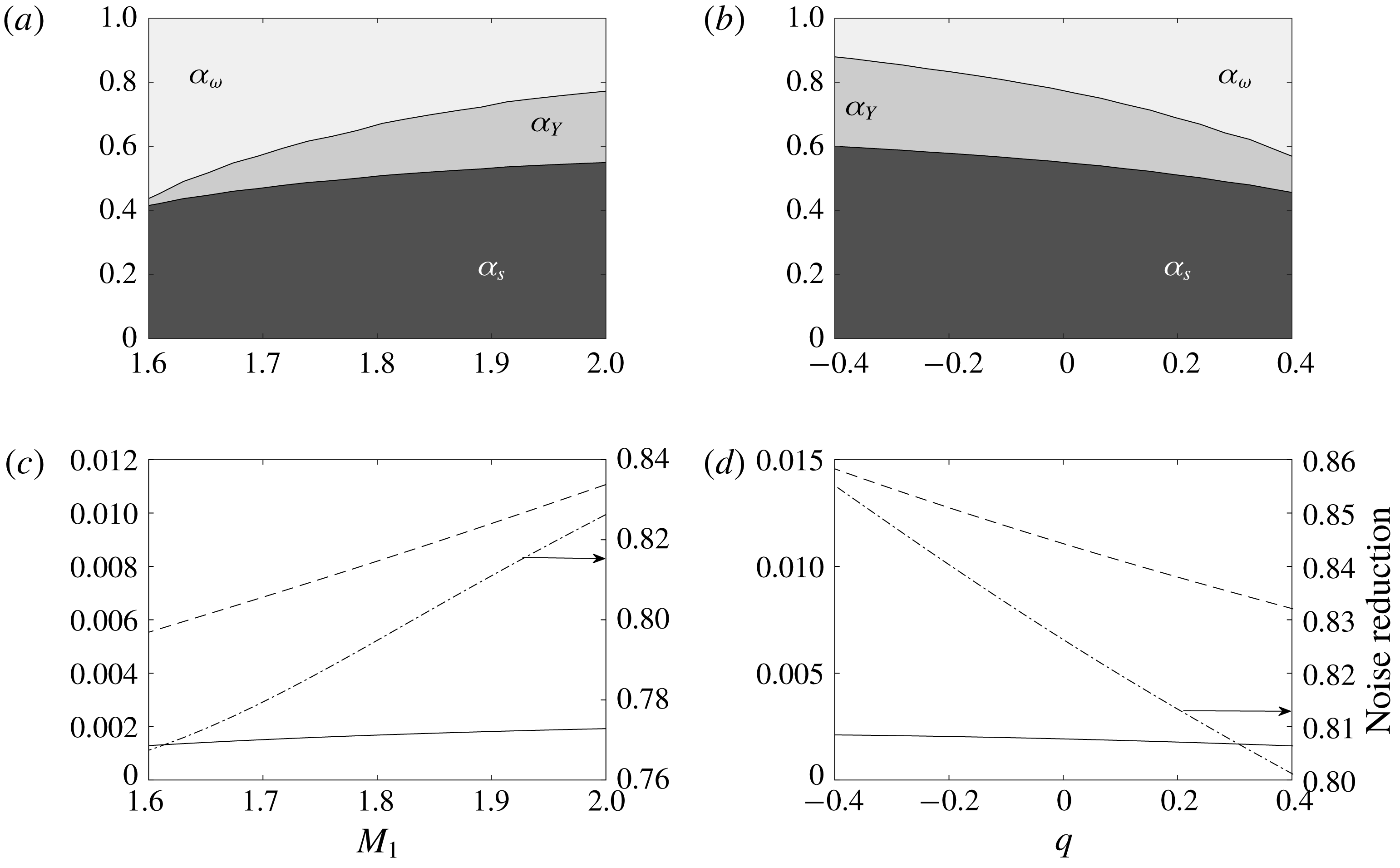
Figure 17. Relative spots amplitudes minimizing the radiated noise
 $\unicode[STIX]{x1D6F1}$
: dependence on
$\unicode[STIX]{x1D6F1}$
: dependence on
 $M_{1}$
for
$M_{1}$
for
 $q=0$
(a), and on
$q=0$
(a), and on
 $q$
for
$q$
for
 $M_{1}=2$
(b). The corresponding integral radiated noise
$M_{1}=2$
(b). The corresponding integral radiated noise
 $\unicode[STIX]{x1D6F1}$
(6.3) is shown for the elementary vortex
$\unicode[STIX]{x1D6F1}$
(6.3) is shown for the elementary vortex
 $\unicode[STIX]{x1D6F1}(0,0)$
(dashed) and the optimal combination
$\unicode[STIX]{x1D6F1}(0,0)$
(dashed) and the optimal combination
 $\unicode[STIX]{x1D6F1}(a_{s},a_{Y})$
(solid) in the bottom two plots (c,d). The dot-dashed lines, plotted with respect to the right axes, show the noise reduction
$\unicode[STIX]{x1D6F1}(a_{s},a_{Y})$
(solid) in the bottom two plots (c,d). The dot-dashed lines, plotted with respect to the right axes, show the noise reduction
 $\unicode[STIX]{x1D6F1}(a_{s},a_{Y})-\unicode[STIX]{x1D6F1}(0,0)/\unicode[STIX]{x1D6F1}(0,0)$
.
$\unicode[STIX]{x1D6F1}(a_{s},a_{Y})-\unicode[STIX]{x1D6F1}(0,0)/\unicode[STIX]{x1D6F1}(0,0)$
.
Figure 18’s top plot shows the resulting pressure field in the case
 $M_{1}=2$
and
$M_{1}=2$
and
 $q=0$
, for which we found
$q=0$
, for which we found
 $a_{Y}=-0.976$
and
$a_{Y}=-0.976$
and
 $a_{s}=2.407$
. It is obtained through linear combination of the emitted pressure for the elementary spots of figures 8, 11 and 14 with weights
$a_{s}=2.407$
. It is obtained through linear combination of the emitted pressure for the elementary spots of figures 8, 11 and 14 with weights
 $(a_{Y},a_{s},1)$
. From the levels of the emitted pressure, it is clear that the radiated noise is significantly reduced compared to either elementary spot – by 82.6 %, as seen in figure 17. Figure 18(b) shows the vorticity pattern downstream of the shock for the same perturbation, following figure 7.
$(a_{Y},a_{s},1)$
. From the levels of the emitted pressure, it is clear that the radiated noise is significantly reduced compared to either elementary spot – by 82.6 %, as seen in figure 17. Figure 18(b) shows the vorticity pattern downstream of the shock for the same perturbation, following figure 7.
Following the above procedure, it is straightforward to minimize other fluctuations, such as vorticity, temperature, etc.
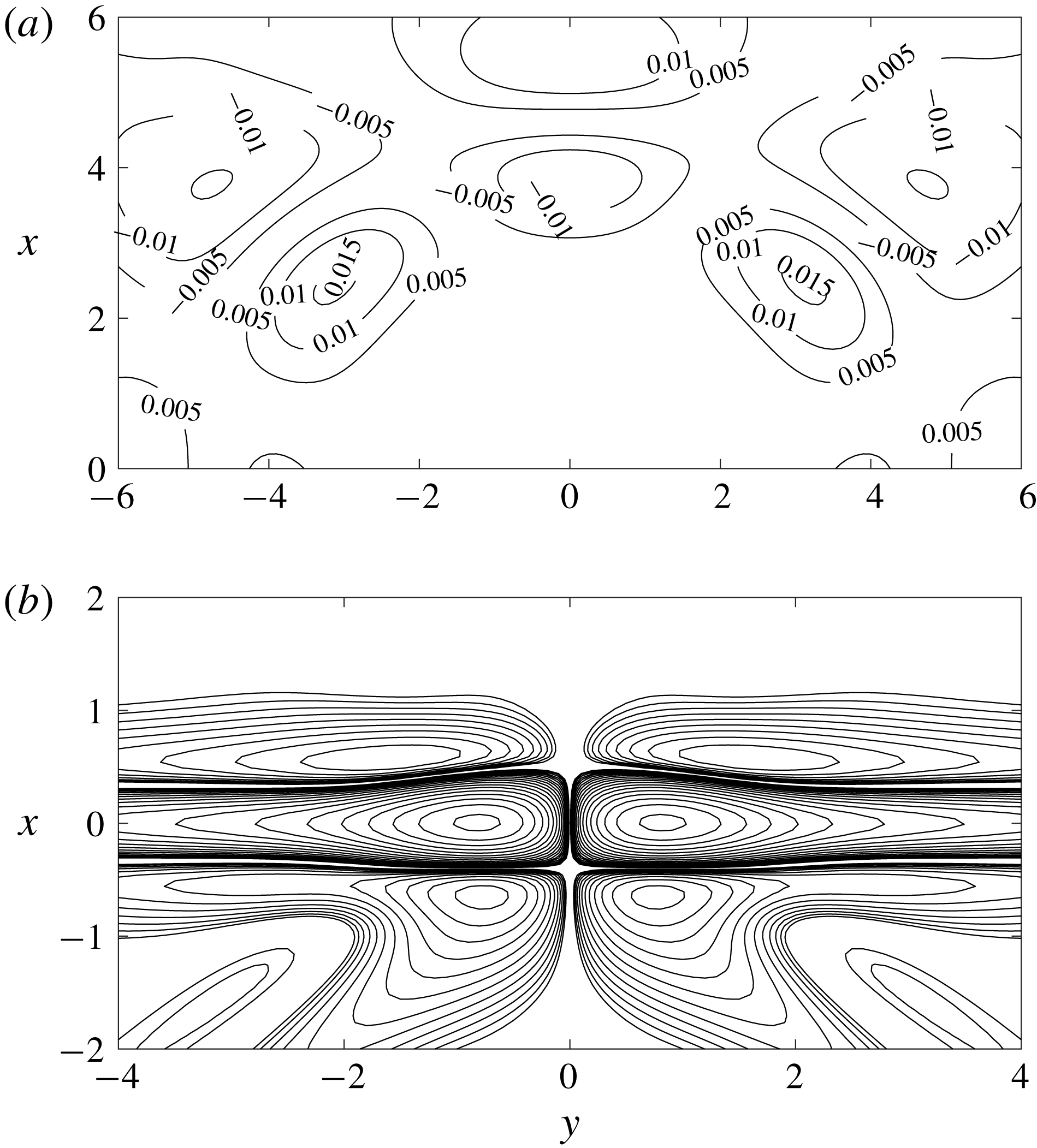
Figure 18. Emitted pressure (a) and vorticity (b) fields for the optimized vortex perturbation minimizing the radiated noise
 $\unicode[STIX]{x1D6F1}$
, in the case
$\unicode[STIX]{x1D6F1}$
, in the case
 $M_{1}=2$
and
$M_{1}=2$
and
 $q=0$
.
$q=0$
.
7 Concluding remarks
A complete LIA framework for the interaction between a planar shock and a Gaussian disturbance including thermal effects at the shock front was proposed, along with adequate extension of the energy of the disturbances. General expressions for the emitted field are also provided, allowing for a straightforward reconstruction of the solution. Such a framework can provide a deep insight into shock/mixed disturbances interaction, but also very accurate benchmark solutions for numerical scheme validation. Another result is the extension of Chu’s definition of disturbance energy to the present framework, leading to a mathematically grounded meaningful definition of the energy of both upstream and downstream fields. It is worth noting that mixed solutions based on the combination of the three elementary solutions analysed in the previous section can also be very easily obtained by linear combinations of the instantaneous elementary fields. This way, some solutions with peculiar features can be obtained. This is illustrated by the search of upstream vortex-like disturbances with minimal emitted pressure perturbations. In a similar way, combining a high density spot with a cold entropy spot one can obtain an emitted field with a very small residual vorticity. Solutions that minimize or maximize the energy of a given emitted Kovásznay mode can be obtained, the relative weight of each upstream mode being a function of the upstream Mach number and the heat source parameter
 $q$
.
$q$
.
With a wide variety of covered shock/spot interaction configurations, this work may serve as benchmark for the development of shock-capturing numerical methods.
Acknowledgements
This work was supported by Labex MEC (ANR-10-LABX-0092) and the A*MIDEX project (ANR-11-IDEX-0001-02), funded by the ‘Investissements d’Avenir’.
Appendix A. Mathematical formulation for Gaussian spot/shock interaction
We address here the general formulation for the upstream and downstream field associated with the interaction between a 2-D Gaussian non-acoustic disturbance and a planar shock within the Kovásznay decomposition framework. The upstream disturbances are advected at the constant speed
 $U$
, and are then frozen in the reference frame moving with the base flow far from the shock wave.
$U$
, and are then frozen in the reference frame moving with the base flow far from the shock wave.
Considering an upstream perturbation of Kovásznay mode
 $i$
of the form (in cylindrical coordinates
$i$
of the form (in cylindrical coordinates
 $(r,\unicode[STIX]{x1D719})$
)
$(r,\unicode[STIX]{x1D719})$
)
 $$\begin{eqnarray}f_{i}(r)=\unicode[STIX]{x1D716}\text{e}^{-r^{2}/D^{2}},\end{eqnarray}$$
where
 $D$
denotes the radius (taken equal to
$D$
denotes the radius (taken equal to
 $1$
) of the Gaussian profile and
$1$
) of the Gaussian profile and
 $f_{i}$
the fluctuation of the physical quantity associated with the Kovásznay mode (e.g. density or specific volume for a density spot, entropy for an entropy spot, vorticity for a vortex), its decomposition into Fourier modes obtained via a 2-D polar Fourier transform is (see Fabre et al. (Reference Fabre, Jacquin and Sesterhenn2001) for a full description of intermediary algebra, with
$f_{i}$
the fluctuation of the physical quantity associated with the Kovásznay mode (e.g. density or specific volume for a density spot, entropy for an entropy spot, vorticity for a vortex), its decomposition into Fourier modes obtained via a 2-D polar Fourier transform is (see Fabre et al. (Reference Fabre, Jacquin and Sesterhenn2001) for a full description of intermediary algebra, with
 $(k,\unicode[STIX]{x1D6FC})$
the polar coordinates in the Fourier space)
$(k,\unicode[STIX]{x1D6FC})$
the polar coordinates in the Fourier space)
 $$\begin{eqnarray}f_{i}(r)=\frac{\unicode[STIX]{x1D716}}{2\unicode[STIX]{x03C0}}\int _{\unicode[STIX]{x1D6FC}=-(\unicode[STIX]{x03C0}/2)}^{\unicode[STIX]{x03C0}/2}K(\hat{r})\,\text{d}\unicode[STIX]{x1D6FC},\end{eqnarray}$$
where
 $$\begin{eqnarray}\displaystyle & \displaystyle K(z)=\int _{k=0}^{\infty }\frac{k}{2}\text{e}^{-(k/2)^{2}}\cos (kz)\,\text{d}k=1-\sqrt{\unicode[STIX]{x03C0}}z\text{e}^{-z^{2}}\text{erfi}(z), & \displaystyle\end{eqnarray}$$
 $$\begin{eqnarray}\displaystyle & \displaystyle \hat{r}=r\cos (\unicode[STIX]{x1D6FC}-\unicode[STIX]{x1D719}). & \displaystyle\end{eqnarray}$$
The complete emitted field is given by
 $$\begin{eqnarray}\displaystyle & \displaystyle \frac{s_{2}^{\prime }}{C_{p2}}=\frac{\unicode[STIX]{x1D716}}{\unicode[STIX]{x03C0}}\,\int _{\unicode[STIX]{x1D6FC}=-(\unicode[STIX]{x03C0}/2)}^{\unicode[STIX]{x03C0}/2}\left[\text{Re}(Z_{is})K\left(\frac{\widehat{r}^{s}}{c}\right)-\text{Im}(Z_{is})L\left(\frac{\widehat{r}^{s}}{c}\right)\right]\,\text{d}\unicode[STIX]{x1D6FC}, & \displaystyle\end{eqnarray}$$
 $$\begin{eqnarray}\displaystyle & \displaystyle \frac{\unicode[STIX]{x1D714}_{2}^{\prime }}{U_{2}}=-\frac{\unicode[STIX]{x1D716}}{\unicode[STIX]{x03C0}}\,\int _{\unicode[STIX]{x1D6FC}=-(\unicode[STIX]{x03C0}/2)}^{\unicode[STIX]{x03C0}/2}\frac{1}{c}\left[\text{Re}(Z_{iv})K^{\prime }\left(\frac{\widehat{r}^{s}}{c}\right)-\text{Im}(Z_{iv})L^{\prime }\left(\frac{\widehat{r}^{s}}{c}\right)\right]\,\text{d}\unicode[STIX]{x1D6FC}, & \displaystyle\end{eqnarray}$$
 $$\begin{eqnarray}\displaystyle & \displaystyle \frac{p_{2}^{\prime }}{\unicode[STIX]{x1D6FE}P_{2}}=\frac{\unicode[STIX]{x1D716}}{2\unicode[STIX]{x03C0}}\text{Re}\left(\int _{\unicode[STIX]{x1D6FC}=-(\unicode[STIX]{x03C0}/2)}^{\unicode[STIX]{x03C0}/2}\int _{k=0}^{\infty }Z_{ia}\text{e}^{-k^{2}/4}\,\text{e}^{-k_{a}\unicode[STIX]{x1D702}(x+M_{2}c_{2}t)}\,\text{e}^{\text{i}\boldsymbol{k}_{a}\boldsymbol{\cdot }\boldsymbol{x}}\,k\,\text{d}k\,\text{d}\unicode[STIX]{x1D6FC}\right), & \displaystyle\end{eqnarray}$$
 $$\begin{eqnarray}\displaystyle & \displaystyle \frac{T_{2}^{\prime }}{T_{2}}=\frac{\unicode[STIX]{x1D716}}{\unicode[STIX]{x03C0}}\,\int _{\unicode[STIX]{x1D6FC}=-(\unicode[STIX]{x03C0}/2)}^{\unicode[STIX]{x03C0}/2}\left[\text{Re}(Z_{is})K\left(\frac{\widehat{r}^{s}}{c}\right)-\text{Im}(Z_{is})L\left(\frac{\widehat{r}^{s}}{c}\right)\right]\text{d}\unicode[STIX]{x1D6FC}+(\unicode[STIX]{x1D6FE}-1)\frac{p_{2}^{\prime }}{\unicode[STIX]{x1D6FE}P_{2}}, & \displaystyle\end{eqnarray}$$
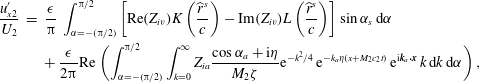 $$\begin{eqnarray}\displaystyle \frac{u_{x2}^{\prime }}{U_{2}} & = & \displaystyle \frac{\unicode[STIX]{x1D716}}{\unicode[STIX]{x03C0}}\,\int _{\unicode[STIX]{x1D6FC}=-(\unicode[STIX]{x03C0}/2)}^{\unicode[STIX]{x03C0}/2}\left[\text{Re}(Z_{iv})K\left(\frac{\widehat{r}^{s}}{c}\right)-\text{Im}(Z_{iv})L\left(\frac{\widehat{r}^{s}}{c}\right)\right]\sin \unicode[STIX]{x1D6FC}_{s}\,\text{d}\unicode[STIX]{x1D6FC}\nonumber\\ \displaystyle & & \displaystyle +\,\frac{\unicode[STIX]{x1D716}}{2\unicode[STIX]{x03C0}}\text{Re}\left(\int _{\unicode[STIX]{x1D6FC}=-(\unicode[STIX]{x03C0}/2)}^{\unicode[STIX]{x03C0}/2}\int _{k=0}^{\infty }Z_{ia}\frac{\cos \unicode[STIX]{x1D6FC}_{a}+\text{i}\unicode[STIX]{x1D702}}{M_{2}\unicode[STIX]{x1D701}}\text{e}^{-k^{2}/4}\,\text{e}^{-k_{a}\unicode[STIX]{x1D702}(x+M_{2}c_{2}t)}\,\text{e}^{\text{i}\boldsymbol{k}_{a}\boldsymbol{\cdot }\boldsymbol{x}}\,k\,\text{d}k\,\text{d}\unicode[STIX]{x1D6FC}\right),\nonumber\\ \displaystyle & & \displaystyle\end{eqnarray}$$
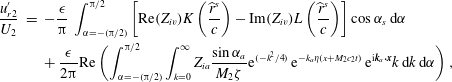 $$\begin{eqnarray}\displaystyle \frac{u_{r2}^{\prime }}{U_{2}} & = & \displaystyle -\frac{\unicode[STIX]{x1D716}}{\unicode[STIX]{x03C0}}\,\int _{\unicode[STIX]{x1D6FC}=-(\unicode[STIX]{x03C0}/2)}^{\unicode[STIX]{x03C0}/2}\left[\text{Re}(Z_{iv})K\left(\frac{\widehat{r}^{s}}{c}\right)-\text{Im}(Z_{iv})L\left(\frac{\widehat{r}^{s}}{c}\right)\right]\cos \unicode[STIX]{x1D6FC}_{s}\,\text{d}\unicode[STIX]{x1D6FC}\nonumber\\ \displaystyle & & \displaystyle +\,\frac{\unicode[STIX]{x1D716}}{2\unicode[STIX]{x03C0}}\text{Re}\left(\int _{\unicode[STIX]{x1D6FC}=-(\unicode[STIX]{x03C0}/2)}^{\unicode[STIX]{x03C0}/2}\int _{k=0}^{\infty }Z_{ia}\frac{\sin \unicode[STIX]{x1D6FC}_{a}}{M_{2}\unicode[STIX]{x1D701}}\text{e}^{(-k^{2}/4)}\,\text{e}^{-k_{a}\unicode[STIX]{x1D702}(x+M_{2}c_{2}t)}\,\text{e}^{\text{i}\boldsymbol{k}_{a}\boldsymbol{\cdot }\boldsymbol{x}}k\,\text{d}k\,\text{d}\unicode[STIX]{x1D6FC}\right),\nonumber\\ \displaystyle & & \displaystyle\end{eqnarray}$$
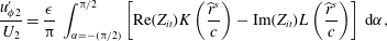 $$\begin{eqnarray}\displaystyle \frac{u_{\unicode[STIX]{x1D719}2}^{\prime }}{U_{2}}=\frac{\unicode[STIX]{x1D716}}{\unicode[STIX]{x03C0}}\,\int _{\unicode[STIX]{x1D6FC}=-(\unicode[STIX]{x03C0}/2)}^{\unicode[STIX]{x03C0}/2}\left[\text{Re}(Z_{it})K\left(\frac{\widehat{r}^{s}}{c}\right)-\text{Im}(Z_{it})L\left(\frac{\widehat{r}^{s}}{c}\right)\right]\,\text{d}\unicode[STIX]{x1D6FC}, & & \displaystyle\end{eqnarray}$$
where it is recalled that
 $\boldsymbol{k}_{a}\boldsymbol{\cdot }\boldsymbol{x}=k_{a}(\cos \unicode[STIX]{x1D6FC}_{a}(x+U_{2}t)+\sin \unicode[STIX]{x1D6FC}_{a}(y-U_{2}t\cot \unicode[STIX]{x1D6FC}_{s}))$
. The auxiliary functions
$\boldsymbol{k}_{a}\boldsymbol{\cdot }\boldsymbol{x}=k_{a}(\cos \unicode[STIX]{x1D6FC}_{a}(x+U_{2}t)+\sin \unicode[STIX]{x1D6FC}_{a}(y-U_{2}t\cot \unicode[STIX]{x1D6FC}_{s}))$
. The auxiliary functions
 $L$
,
$L$
,
 $K^{\prime }$
,
$K^{\prime }$
,
 $L^{\prime }$
,
$L^{\prime }$
,
 $\widehat{r}^{s}$
and
$\widehat{r}^{s}$
and
 $c$
are defined as
$c$
are defined as
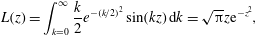 $$\begin{eqnarray}\displaystyle & \displaystyle L(z)=\int _{k=0}^{\infty }\frac{k}{2}e^{-(k/2)^{2}}\sin (kz)\,\text{d}k=\sqrt{\unicode[STIX]{x03C0}}z\text{e}^{-z^{2}}, & \displaystyle\end{eqnarray}$$
 $$\begin{eqnarray}\displaystyle & \displaystyle K^{\prime }(z)=-2z-\sqrt{\unicode[STIX]{x03C0}}(1-2z^{2})\text{e}^{-z^{2}}\text{erfi}(z), & \displaystyle\end{eqnarray}$$
 $$\begin{eqnarray}\displaystyle & \displaystyle L^{\prime }(z)=\sqrt{\unicode[STIX]{x03C0}}(1-2z^{2})\text{e}^{-z^{2}}, & \displaystyle\end{eqnarray}$$
 $$\begin{eqnarray}\displaystyle & \displaystyle c=\frac{\sin \unicode[STIX]{x1D6FC}_{s}}{\sin \unicode[STIX]{x1D6FC}},\quad \widehat{r}^{s}=r\cos (\unicode[STIX]{x1D6FC}_{s}-\unicode[STIX]{x1D719}). & \displaystyle\end{eqnarray}$$
The emitted density field
 $\unicode[STIX]{x1D70C}_{2}^{\prime }$
and specific volume
$\unicode[STIX]{x1D70C}_{2}^{\prime }$
and specific volume
 $\unicode[STIX]{x1D70F}_{2}^{\prime }=1/\unicode[STIX]{x1D70C}_{2}^{\prime }$
are computed for each component from
$\unicode[STIX]{x1D70F}_{2}^{\prime }=1/\unicode[STIX]{x1D70C}_{2}^{\prime }$
are computed for each component from
 $T^{\prime }$
,
$T^{\prime }$
,
 $Y^{\prime }$
and
$Y^{\prime }$
and
 $p^{\prime }$
in a straightforward way using the linearized equation of state, i.e.
$p^{\prime }$
in a straightforward way using the linearized equation of state, i.e.
 $$\begin{eqnarray}\displaystyle \frac{p^{\prime }}{P}=\frac{\unicode[STIX]{x1D70C}^{\prime }}{\unicode[STIX]{x1D70C}}+\frac{T^{\prime }}{T}+A_{t}^{r}Y^{\prime }. & & \displaystyle\end{eqnarray}$$


