2.1 Non-dimensional filament parameters

If the filaments are placed densely, the mean fluid velocity inside the bed is very small. The slow flow inside bed means that the force on the filament tips is much larger than the force on the body of the filaments, $F_{tip}\gg f_{body}l$ . This estimation is discussed more quantitatively in appendix A. The wall-shear stress of the actual wall, to which the filaments are attached, is negligible. The filament tip force in the streamwise direction can therefore be approximated by the fluid shear stress, $\unicode[STIX]{x1D70F}$ , on the top face of the cell coinciding with the $y=0$ plane (see figure 1),

(2.4) $$\begin{eqnarray}F_{tip}\approx \int _{cell\,face}\unicode[STIX]{x1D70F}\,\text{d}x\,\text{d}z.\end{eqnarray}$$

Next, we non-dimensionalise the filament equation by defining $q^{\ast }=q/a$ , $y^{\ast }=y/l$ , $t^{\ast }=t/T_{f}$ and $F_{tip}^{\ast }=F_{tip}/\langle F_{tip}\rangle$ . The filament displacement is thus assumed to scale with the radius, $a$ , whereas the characteristic length scale in the wall-normal direction is $l$ . We have also introduced a reference time scale $T_{f}$ and a characteristic tip force magnitude $\langle F_{tip}\rangle$ . Henceforth, $\langle \cdot \rangle$ will be used to denote the mean value of a quantity. In dimensionless variables, we have

(2.5) $$\begin{eqnarray}\frac{\unicode[STIX]{x2202}^{4}q^{\ast }}{\unicode[STIX]{x2202}{y^{\ast }}^{4}}+{T^{\ast }}^{2}\frac{\unicode[STIX]{x2202}^{2}q^{\ast }}{\unicode[STIX]{x2202}{t^{\ast }}^{2}}=0\end{eqnarray}$$

and $q^{\ast }=0$ , $\unicode[STIX]{x2202}q^{\ast }/\unicode[STIX]{x2202}y^{\ast }=0$ at $y^{\ast }=-1$ and $\unicode[STIX]{x2202}^{2}q^{\ast }/\unicode[STIX]{x2202}{y^{\ast }}^{2}=0$ , $\unicode[STIX]{x2202}^{3}q^{\ast }/\unicode[STIX]{x2202}{y^{\ast }}^{3}=-Q^{\ast }F_{tip}^{\ast }$ at $y^{\ast }=0$ . We obtain two non-dimensional numbers, namely,

(2.6) $$\begin{eqnarray}T^{\ast }=\frac{T}{T_{f}}=\frac{1}{T_{f}}\left(l^{2}\sqrt{\frac{\unicode[STIX]{x1D70C}_{s}A+\unicode[STIX]{x1D712}}{EI}}\right)\end{eqnarray}$$

and

(2.7) $$\begin{eqnarray}Q^{\ast }=\frac{Q}{a}=\frac{\langle F_{tip}\rangle l^{3}}{EIa}.\end{eqnarray}$$

The latter number represents a Cauchy number, which describes the static deformation under the effect of shear force, i.e. $Q^{\ast }\sim \langle q^{\ast }(0,t)\rangle$ , where $\langle q^{\ast }(0,t)\rangle$ is the non-dimensional mean displacement of the filament tip. Therefore, we may expect a bending of the filament under an external tip force $\langle F_{tip}\rangle$ when the filament is sufficiently long and soft so that $Q^{\ast }\sim 1$ . The displacement of the tip is henceforth denoted with a tilde, so that $\tilde{q}(t)=q(0,t)$ .

The second non-dimensional number $T^{\ast }$ is commonly referred to as the reduced velocity. The numerator $T$ is proportional the period of natural free vibrations of a filament,

(2.8) $$\begin{eqnarray}T_{n}=\unicode[STIX]{x1D6FC}l^{2}\sqrt{\frac{A\unicode[STIX]{x1D70C}_{s}+\unicode[STIX]{x1D712}}{EI}},\end{eqnarray}$$

where $\unicode[STIX]{x1D6FC}=2\unicode[STIX]{x03C0}/1.875^{2}$ . Therefore, sufficiently light and stiff filaments with $T<T_{f}$ are quick to adapt to external changes on the time scale $T_{f}$ . On the other hand, very heavy and soft filaments with $T>T_{f}$ are expected to adapt comparatively slow. A strong fluid–structure interaction is thus expected when both $T^{\ast }$ and $Q^{\ast }$ are order one.

Figure 2. Black solid lines represent a schematic of the transfer function between the forcing and the displacement of heavy/soft filaments (a) and light/stiff filaments (b). The natural frequency is approximately $1/T$ , and the mean displacement is $\langle \tilde{q}\rangle$ . The grey line represents the frequency-weighted wall-shear stress spectrum of a turbulent channel flow, which reaches its peak value at $1/T_{f}$ .

2.2 Estimates of turbulent scales

In order to determine $Q^{\ast }$ and $T^{\ast }$ for a given filamentous bed, we need to estimate the mean force $\langle F_{tip}\rangle$ and a characteristic forcing time scale $T_{f}$ for a turbulent flow. The former can be estimated from the wall-shear stress,

(2.9) $$\begin{eqnarray}\langle F_{tip}\rangle =\unicode[STIX]{x1D70F}_{wall}s^{2}=\unicode[STIX]{x1D70C}\frac{Re_{\unicode[STIX]{x1D70F}}^{2}\unicode[STIX]{x1D708}^{2}}{h^{2}}s^{2}.\end{eqnarray}$$

The forcing time scale $T_{f}$ , related to the force imposed on the filaments from the flowing fluid ( $F_{tip}$ ), can be estimated from numerical simulations. The frequency content of the streamwise and spanwise wall-shear stress for turbulent channel flows with smooth walls are of broadband character. However, there is a range of frequencies that dominate and which are related to the passing of turbulent structures (e.g. streaks, vortices). Hu et al. (Reference Hu, Morfey and Sandham2006) computed frequency-weighted wall-shear stress spectra for $Re_{\unicode[STIX]{x1D70F}}=180$ (and higher Reynolds numbers). Their spectra represent the energy content of the wall-shear stress for different frequencies. A sketch of one spectrum is shown in figure 2 (grey line). For low frequencies, the frequency-weighted wall-shear stress increases almost linearly, with a derivative of one in wall units, up to a peak. The peaks are found at $f^{+}=0.012$ and $f^{+}=0.037$ , for the streamwise and spanwise components respectively. Here, $f^{+}=\unicode[STIX]{x1D708}/(T_{f}u_{\unicode[STIX]{x1D70F}}^{2})$ . Due to the linear increase, the energy is practically negligible one decade below the peak. The magnitude of frequencies larger than the peak decrease rapidly, and the energy above $f^{+}=0.2$ is very small, for both components.

The forcing on a filament bed is thus dominated by frequencies around $f^{+}=0.01$ , and different fluid–surface interaction behaviour can be expected, depending on the reduced velocity $T^{\ast }=T/T_{f}$ , as schematically shown in figure 2. If the time scale of the filaments is much larger than $T_{f}$ , i.e. $T\gg T_{f}$ (figure 2 a), the filaments have no time to respond to the forcing and thus behave as rigid. At the other extreme, a bed of filaments with $T\ll T_{f}$ (figure 2 b) will quickly adapt to the forcing and thus equilibrate.

We will in § 4 look at two surfaces whose time scales $T^{\ast }$ differ nearly by an order of magnitude, but whose expected filament displacements are of the same order of magnitude, i.e. $\langle \tilde{q}\rangle /a=0.64$ . This is illustrated schematically in figure 2. In this work, we assume that the bed geometry (set by $a$ , $l$ and $s$ ) is fixed; therefore and as apparent from (1.1) the expected mean deflection, $Q^{\ast }$ – determined by $E$ – and the expected time scale ratio, $T^{\ast }$ – determined by both $E$ and $\unicode[STIX]{x1D70C}_{s}$ – can be chosen independently.

2.3 Investigated configurations

To characterise the interaction between turbulence and a filament bed for different filament time scales, we perform a number of simulations (table 1). For all simulations, a fixed filament radius is used, which in wall units corresponds to $a^{+}\approx 2$ , with exact equality when $Re_{\unicode[STIX]{x1D70F}}=180$ . The aspect ratio of the filaments we set to $l/a=10$ . Two cases of rigid filaments are investigated: one with a centre-to-centre distance of $s/a=4$ and one with $s/a=8$ , denoted as A and B, respectively. In addition to these, six flexible filaments configurations are investigated (I–VI), with two different mean displacements, $\langle \tilde{q}\rangle$ , and three different natural frequencies, $f_{n}$ .

Table 1. Geometric and dynamic properties of the configurations that are investigated. For all configurations, the radius is $a^{+}=2$ and the aspect ratio is $l/a=10$ . The non-dimensional numbers $Q^{\ast }=3\langle \tilde{q}\rangle /a$ and $T^{\ast }=\unicode[STIX]{x1D6FC}^{-1}T_{n}/T_{f}$ , where $\unicode[STIX]{x1D6FC}=2\unicode[STIX]{x03C0}/1.875^{2}\approx 1.8$ . The mean displacements $\langle \tilde{q}\rangle$ are calculated from (5.2) and the frequencies $f_{n}^{+}$ from (2.8). Two of the cases have rigid filaments, namely A and B. For the cases with flexible filaments, I–VI, two mean displacement amplitudes are considered and for each mean displacement, three different resonance frequencies are investigated. For the quantities scaled in wall units and for estimation of the wall-shear stress, the friction Reynolds number $Re_{\unicode[STIX]{x1D70F}}=180$ is used. The time scale ratio (reduced velocity) considers the natural frequency of the filaments and the frequency of the maximum frequency-weighted streamwise wall-shear stress.

3.1 Fluid solver

The lattice-Boltzmann method (LBM) is a discretisation of the Boltzmann kinetic equation. However, only the necessary details of molecular motion are retained in order to recover macroscopic conservation laws of mass, momentum and energy (Krüger et al. Reference Krüger, Kusumaatmaja, Kuzmin, Shardt, Silva and Viggen2017). In the LBM, the spatial dimensions are discretised on a grid and the particle velocity space into a set of discrete velocities. With $d$ spatial dimensions and the velocity set having a size $q$ , the velocity set is denoted by D $d$ Q $q$ . We use the D3Q19 set, together with the Bhatnagar–Gross–Krook (BGK) collision operator, on grids with cubic cells. The implementation is based on the Palabos library (Chopard et al. Reference Chopard, Kontaxakis, Lagrava, Latt, Malaspinas, Parmigiani, Rybak and Sagon2015).

Table 2. Grids used for validation and in simulations. The resolution of different grid refinements together with the properties of the Lagrangian grid of the filaments are specified. G1 and G2 have one grid refinement at each wall, whereas G3 has one additional refinement at the lower wall. Friction Reynolds number $Re_{\unicode[STIX]{x1D70F}}=180$ is used for scaling in wall units.

The dimensions of the computational domain are $6.3h\times 2h\times 2.1h$ for simulations of smooth wall channels presented below and $6.3h\times (2h+l)\times 2.1h$ for the simulations with filaments. Grids with the different resolutions are denoted by G1, G2 and G3, respectively, and are listed in table 2. The grid G1 is used for the results presented in §§ 4 and 5. For this grid, the resolution is $\unicode[STIX]{x1D6FF}x^{+}=2$ for $Re_{\unicode[STIX]{x1D70F}}=180$ , giving a grid size of $568\times 181\times 190$ . However, the grid is refined with a factor of two at the upper and lower walls, up to $y^{+}\approx 40$ . The refinements are made with an overlap of one coarse grid spacing as described by Lagrava et al. (Reference Lagrava, Malaspinas, Latt and Chopard2012). To minimise mass and momentum imbalances, a correction step is included before the collision step at the interface nodes, similar to the method described by Kuwata & Suga (Reference Kuwata and Suga2016), however adapted to overlapping nodes. As is commonly done in LBM simulations of channel flows, we use a constant applied pressure gradient to drive the flow, implemented with the Guo forcing scheme (Guo, Zheng & Shi Reference Guo, Zheng and Shi2002). At the walls, the wet-node regularised boundary condition is used (Latt et al. Reference Latt, Chopard, Malaspinas, Deville and Michler2008).

Figure 3. Statistics of a channel flow computed using the LBM employed in this work and computed using a spectral scheme (Lee & Moser Reference Lee and Moser2015). The (a) mean velocity, (b) velocity fluctuations, (c) Reynolds shear stress and (d) pressure fluctuations are shown. The agreement is considered satisfactory; errors are within a few per cent for the two grids G1 and G2 when compared to the spectral results.

To validate the fluid solver, we compare a fully developed channel flow with smooth walls to the spectral DNS by Lee & Moser (Reference Lee and Moser2015). Two grids are used: G1 and G2, listed in table 2. Due to the symmetry of the problem, the results from the two sides can be averaged. Figure 3 compares the mean velocity, root-mean-square (r.m.s.) velocities, Reynolds shear stress (RSS) and r.m.s. pressure to the spectral results.

Close to the wall, the r.m.s. values of velocity and pressure fluctuations of the two grids G1 and G2 agree within 2 %, indicating grid convergence. Comparing the r.m.s. velocities and the RSS to the spectral results, the largest differences are around 3 %. For the pressure fluctuations, however, the difference at the wall is slightly larger, around 3.6 %. In the spectral DNS, the pressure is merely a product of the velocity field, whereas in the LBM it is a result of the density fluctuations. This may therefore result in a local violation of mass conservation at the wall, possibly originating from the boundary condition. Although there exist more sophisticated boundary conditions (Dorschner et al. Reference Dorschner, Chikatamarla, Bösch and Karlin2015), we regard the current level of accuracy acceptable for a time scale analysis.

3.2 Solid solver

The fluid–solid interaction is described by an immersed boundary approach, known as the external boundary force method (EBFM) (Wu & Aidun Reference Wu and Aidun2010b ). This method uses a force to enforce the no-slip and impermeability conditions, modelling the surface of a solid object. Surfaces of solid objects are discretised with a Lagrangian grid. This method has been used earlier to simulate fibre suspensions, both flexible and rigid, by Wu & Aidun (Reference Wu and Aidun2010a ) and Do-Quang et al. (Reference Do-Quang, Amberg, Brethouwer and Johansson2014); the current implementation is based on the one by Do-Quang et al. (Reference Do-Quang, Amberg, Brethouwer and Johansson2014). The conversion of quantities between the Eulerian grid of the fluid and the Lagrangian grid of the filaments is performed with a discretisation of the Dirac delta function (Peskin Reference Peskin2002).

Figure 4. Schematic illustration of the Lagrangian grid of a filament. Hinges (green) are connected by rods (blue), and each hinge has a ring of Lagrangian nodes (red). There are also additional nodes on the tip of the filament.

In the current investigation, the dynamic Euler–Bernoulli equation (2.1) is discretised in a rod–hinge fashion, described below. The structure of the grid is shown in figure 4. This model was introduced by Schmid, Switzer & Klingenberg (Reference Schmid, Switzer and Klingenberg2000) and developed further by Lindström & Uesaka (Reference Lindström and Uesaka2007), Wu & Aidun (Reference Wu and Aidun2010a ) and Do-Quang et al. (Reference Do-Quang, Amberg, Brethouwer and Johansson2014). A similar model, using chains of spheres, was introduced by Yamamoto & Matsuoka (Reference Yamamoto and Matsuoka1993) and a model using chains of spheroids was introduced by Ross & Klingenberg (Reference Ross and Klingenberg1997). These models can be used both to describe flexible and rigid fibres.

A filament has $N_{h}$ hinges, with $N_{n}$ Lagrangian grid nodes in a ring around each hinge, together with $N_{n}^{lid}$ additional nodes on the lid. At the hinges, the filaments can deflect. The hinges of a filament are connected by rods and these can be extended or compressed. Hence, the filaments are extensible, however in practice the extensions and compressions of the rods are small, typically below 1 %. The direction of the rod between hinge $i-1$ and $i$ is parallel to the tangent unit vector

(3.1) $$\begin{eqnarray}\boldsymbol{p}_{i}=\frac{\boldsymbol{x}_{i}-\boldsymbol{x}_{i-1}}{\Vert \boldsymbol{x}_{i}-\boldsymbol{x}_{i-1}\Vert },\end{eqnarray}$$

where $\boldsymbol{x}_{i}$ is the location of hinge $i$ and $\Vert \cdot \Vert$ denotes the Euclidean norm. The first rod is assumed to be fixed to the wall, so that $\boldsymbol{p}_{1}=(0,1,0)^{\text{T}}$ , and for the last one we impose $\boldsymbol{p}_{N_{h}+1}=\boldsymbol{p}_{N_{h}}$ .

In the Euler–Bernoulli equation, the bending moment of a beam, $M$ , is assumed to be proportional to the curvature, $\unicode[STIX]{x1D705}$ , and the stiffness, giving $M=EI\unicode[STIX]{x1D705}$ , where $\unicode[STIX]{x1D705}=\unicode[STIX]{x2202}^{2}q/\unicode[STIX]{x2202}y^{2}$ . For the rod–hinge model, the bending moment across hinge $i$ can be evaluated as

(3.2) $$\begin{eqnarray}\boldsymbol{M}_{i}=EI\frac{\arccos (\,\boldsymbol{p}_{i+1}\boldsymbol{\cdot }\boldsymbol{p}_{i})}{l_{r}}\frac{\boldsymbol{p}_{i+1}\times \boldsymbol{p}_{i}}{\Vert \boldsymbol{p}_{i+1}\times \boldsymbol{p}_{i}\Vert },\end{eqnarray}$$

where the first fraction is an estimation of the local curvature and the last fraction gives the direction. Considering an infinitesimal beam element, there is a local balance between the bending moment and the torque that the shear force, $S$ , gives rise to, $S=\unicode[STIX]{x2202}M/\unicode[STIX]{x2202}y$ . In our discrete model, however, we are not interested in the shear force, but the resulting force on a discrete segment of length $l_{r}$ , corresponding to the length of a rod or one hinge. This force, $F$ , is given by the change in the shear force over a length $l_{r}$ . Using a linear approximation, $F=l_{r}\unicode[STIX]{x2202}S/\unicode[STIX]{x2202}y=l_{r}\unicode[STIX]{x2202}^{2}M/\unicode[STIX]{x2202}y^{2}$ . It can be noted that with the estimation of the curvature as the second derivative of the displacement, $F=l_{r}EI\unicode[STIX]{x2202}^{4}q/\unicode[STIX]{x2202}y^{4}$ , which corresponds to the first term in the Euler–Bernoulli equation (2.1). We approximate this force by central differences, taking into account the direction of the rods,

(3.3) $$\begin{eqnarray}\boldsymbol{F}_{i}^{h}=\frac{\boldsymbol{M}_{i-1}\times \boldsymbol{p}_{i}}{l_{r}}+\frac{\boldsymbol{M}_{i+1}\times \boldsymbol{p}_{i+1}}{l_{r}}-\frac{\boldsymbol{M}_{i}\times (\,\boldsymbol{p}_{i+1}+\boldsymbol{p}_{i})}{l_{r}}.\end{eqnarray}$$

For the end hinge, the terms including $\boldsymbol{p}_{i+1}$ are removed.

Table 3. Predicted static displacement, computed using the static Euler–Bernoulli equation, and measured static deflection using the considered rod–hinge model. The measured static deflection was approximated as the displacement of the top hinge.

When a rod is compressed or extended by a fractional change in length $\unicode[STIX]{x1D716}$ , it results in a stress given by Hook’s law, $\unicode[STIX]{x1D70E}=E\unicode[STIX]{x1D716}$ . The resulting force on a hinge, corresponding to this stress, is

(3.4) $$\begin{eqnarray}\boldsymbol{F}_{i}^{r}=-EA\frac{\Vert \boldsymbol{x}_{i}-\boldsymbol{x}_{i-1}\Vert -l_{r}}{l_{r}}\boldsymbol{p}_{i}+EA\frac{\Vert \boldsymbol{x}_{i+1}-\boldsymbol{x}_{i}\Vert -l_{r}}{l_{r}}\boldsymbol{p}_{i+1}.\end{eqnarray}$$

For the end hinge only the first term remains.

The force from the fluid, $\boldsymbol{F}_{i}^{fluid}$ , is calculated by summing the fluid forces on the ring of Lagrangian nodes, given by the EBFM. For the top hinge, the forces on the additional nodes of the lid are included. The ring of nodes at each hinge is tilted so that its normal is $(\,\boldsymbol{p}_{i+1}+\boldsymbol{p}_{i})/\Vert \boldsymbol{p}_{i+1}+\boldsymbol{p}_{i}\Vert$ . The total force on a hinge is then $\boldsymbol{F}_{i}=\boldsymbol{F}_{i}^{h}+\boldsymbol{F}_{i}^{r}+\boldsymbol{F}_{i}^{fluid}$ , and the boundary condition implies that the total force on the first hinge is zero, $\boldsymbol{F}_{1}=0$ . With the explicit expression for the force on the hinges, the acceleration of each hinge can be calculated and they can be advected with the corresponding velocity.

The filament model has been validated in the static limit by applying a tip force at the top hinge and comparing it to the analytical prediction from the Euler–Bernoulli equation (2.1). This was done for the geometrical parameters in table 1 and four different deflection amplitudes. The results are summarised in table 3, with errors around 9 % for smaller deflections ( $\tilde{q}\lesssim a$ ), measuring the deflection of the top hinge. The deviation is slightly higher for the case of $\tilde{q}=3a$ (14 %). However the analytical prediction – in contrast to the rod–hinge model – neglects the contribution from the first derivative of the displacement in the curvature and does not correct for the displacement of the beam in the vertical direction (Bisshopp & Drucker Reference Bisshopp and Drucker1945). It therefore loses accuracy for deflections comparable to the length of the filament ( $l=10a$ ). Accounting for this, the error is reduced to 7 %. The error can be further reduced to approximately 1 %, if accounting for the small deviation between the top hinge and the actual tip of the filament (see figure 4). We thus find the hinge–rod model as a reasonable numerical description of Euler–Bernoulli-type of filaments. We characterised the dynamic response of a filament by measuring the natural frequency in the step response of an applied tip force. For both cases I and III, the difference between the measured and the predicted frequency (by (2.8)) was less than 1 %.

A grid refinement study was also performed to validate the fluid–solid interaction under turbulent conditions. For this study, we use the grids G1 and G3, having $\unicode[STIX]{x1D6FF}x^{+}\approx 1$ and $\unicode[STIX]{x1D6FF}x^{+}\approx 0.75$ near the filamentous wall, respectively (see table 2). For case III, the drag and the r.m.s. velocities were increased by around 5–6 % using G3. When it comes to identifying different fluid–surface interaction regimes by varying the time scale ratio $T/T_{f}$ , we find the accuracy provided by G1 acceptable.

4.1 Bed response

For the heavy bed (case I), the force on one filament is shown in figure 6(a), the displacement of the same filament in 6(b) and the power spectral density (PSD) of the force in 6(c). We employ standard spectral analysis for the estimation of the spectra (Brandt Reference Brandt2011), however a short summary is provided in appendix B. From the time series, the strong low pass filtering property of the heavy filamentous bed is apparent: the force in figure 6(a) contains a large range of frequencies, while the filament movement in figure 6(b) is dominated by the resonance frequency and lower frequencies. The mean streamwise displacement, $Q=0.58a$ (blue dashed line in figure 6 b), is close to the displacement (red dotted line) estimated from expression (5.2). Around the mean, we observe from figure 6(b) nearly periodic fluctuations of the filaments with a time period of $T_{f}^{+}\approx 300$ which corresponds to $f^{+}=0.004$ (dashed vertical line in figure 6 c). This can be compared to the resonance frequency estimated from (2.8), $f^{+}=0.0080$ (red dotted vertical line in figure 6 c). It is thus clear that the slow response of the bed is dominated by the low resonance frequency of the filaments. We note that the tip force occasionally attains a negative value due to the interaction between adjacent filaments.

Corresponding figures for case III are shown in figure 6(d–f). This bed is lighter and thus also much faster, which can clearly be observed from the high correlation between the signals in figures 6(d) and 6(e). The correlation coefficient (Freund, Wilson & Mohr Reference Freund, Wilson and Mohr2010) between the displacement and the tip force in the streamwise direction was found to be $r_{\text{III}}=0.71$ , while for I it was $r_{\text{I}}=0.24$ . The lower correlation coefficient of I reflects its slower and more resonant filaments. The dominant measured frequency of the forcing (dashed vertical line in figure 6 f) is $f^{+}\approx 0.03$ , whereas the frequency estimated from (2.8) is $f^{+}=0.057$ (red dotted vertical line in figure 6 f).

Table 4. The friction Reynolds number of the wall with filaments, $Re_{\unicode[STIX]{x1D70F}}^{f}$ , the global drag increase, $\unicode[STIX]{x0394}D$ , and r.m.s. values of the filament displacements obtained from numerical simulations of cases A, B, I–VI.

The r.m.s. values of the streamwise and spanwise displacements are

(4.4) $$\begin{eqnarray}\left.\begin{array}{@{}c@{}}(\tilde{q}_{x},\tilde{q}_{z})_{rms}=(2.61,1.39)a\quad \text{for I and}\\ (\tilde{q}_{x},\tilde{q}_{z})_{rms}=(0.90,0.87)a\quad \text{for III,}\end{array}\right\}\end{eqnarray}$$

as reported in table 4. For case I, the streamwise r.m.s. value is almost twice the spanwise value, whereas for III they are similar. The small difference of the two components for III indicates a high isotropy of the forcing and thus of the fluid velocity fluctuations. This difference can be understood in more detail by comparing the wall-normal displacement field for cases I and III, respectively, at one time instant (figure 7). The wall-normal displacement is a consequence of the spanwise and streamwise displacement, since in practice, the filaments are inextensible; it thus provides a measure of the total displacement. The displacement field of I is dominated by large streamwise structures, similar to streaks, while for III, there are no such structures and the field is relatively isotropic. Further statistical information of the filament motion is provided in figure 8, showing contours of the probability density function (PDF) of the displacement in the $xz$ -plane for I (8 a) and III (8 b). As indicated by the displacement r.m.s. values, the displacements of the filaments in I are much larger in the streamwise direction than the spanwise direction. For III, the distribution is similar in the streamwise and spanwise directions.

Figure 7. Wall-normal filament deformation, $\tilde{q}_{y}/a$ , i.e. at the plane $y=0$ , for (a) case I and (b) case III, at one time instant. For case I, low frequency streaky structures are apparent, whereas the deformation field of case III is more isotropic.

Figure 8. Contours of the probability density function of the filament tip displacement, $\tilde{\boldsymbol{q}}$ , in the $xz$ -plane, for case (a) I and (b) III. Areas of high probability density are yellow, whereas areas of low probability density are blue. The mean displacement is marked with a red cross. The slight asymmetry of the probability density of I in the spanwise direction is attributed to the finite size of the sample.

From figure 7, it can be observed that the displacement field of I has a streak-like structure, whereas III has a much more isotropic displacement field. For the slow and heavy bed, adjacent filaments move in phase, creating the streamwise elongated streaky structures. Generally, for a smooth surface, the spanwise spacing between streaks is approximately $\unicode[STIX]{x0394}z^{+}=100$ , corresponding to $\unicode[STIX]{x0394}z=0.5h$ , whereas the length of streaks is around $\unicode[STIX]{x0394}x^{+}=1000$ , corresponding to $\unicode[STIX]{x0394}x=5h$ (Pope Reference Pope2001). This is similar to what is observed for case I in figure 7(a). Also, for I, the time scale of the filament movement has the same order of magnitude as the passing of a streak: considering the speed of a high speed streak to be around $u^{+}=3$ (from figure 11 a), the streak travels a distance $\unicode[STIX]{x0394}x^{+}=800$ during one period of oscillation of a filament at the resonance frequency.

Figure 9. (a) Zoomed-in top view of an event of large filament displacements for case III, with the direction of mean flow to the right. The centre-to-centre distance at the filament tips is locally enlarged, increasing the permeability. (b) The probability density function of the centre-to-centre distance in the spanwise direction, $s_{tip,z}$ , for III (——) and I (– – –).

For case III, figure 7(b) reveals localised regions of relatively large displacements, around $\unicode[STIX]{x0394}x=0.5h$ in size. This size corresponds to $10s$ , where $s$ is the centre-to-centre distance of the filaments. These regions of separated filaments are created by fluctuations with negative wall-normal velocity moving towards the wall, similar to sweep events. A zoomed-in view of the filaments at such an event is shown in figure 9(a). We observe that these events create centre-to-centre distances of the filament tips in the spanwise direction, $s_{tip,z}$ , up to $8a$ . Therefore, these patches have a higher permeability, increasing locally the transport of mass and momentum from the free flow to the bed. The PDF of $s_{tip,z}$ is presented in figure 9(b). The mean is $\langle s_{tip,z}\rangle =s$ , and $s_{tip,z}$ is constrained to be larger than one filament diameter, $2a$ . This can be compared to the corresponding PDF of case I, where we observe a tighter distribution around the mean $s=4a$ .

We do not observe any clear evidence of periodic vortex shedding due to filaments; there is no common peak in the spectra of the forcing for the different cases that could relate to such events (compare figures 6 c and 6 f). Vortex separation also seems improbable from an estimation of the Reynolds number based on the filament diameter.

4.2 Turbulence modification

Having discussed the behaviour of the filament movement of cases I and III in § 4.1, we here discuss the modification of turbulence over the two beds. In order to separate the contributions of a permeable surface from a deformable surface, we will also compare the turbulence modifications to that of the rigid but permeable configurations, A and B. Case A has the same geometry as I and III, whereas B has twice the filament centre-to-centre distance, namely $s=8a$ , and thus a higher permeability than A (the permeability scales with $s^{2}$ ).

4.2.1 Drag characteristics

A first quantification of the effects of the filaments on the turbulence can be done by measuring the change in drag. The local drag increase of the filament wall can be characterised by $Re_{\unicode[STIX]{x1D70F}}^{f}=u_{\unicode[STIX]{x1D70F}}^{f}h/\unicode[STIX]{x1D708}$ . From the tabulated data in table 4, we observe that the friction Reynolds number for the slow bed (case I) is very close to that of the smooth channel ( $Re_{\unicode[STIX]{x1D70F}}=180$ ), whereas for the fast bed (case III) we have $Re_{\unicode[STIX]{x1D70F}}^{f}=200$ . Interestingly, the rigid configuration with higher permeability (case B) has a friction Reynolds number ( $Re_{\unicode[STIX]{x1D70F}}^{f}=204$ ) very close to case III, giving a first indication that B and III modify the near-wall turbulence in a similar way.

The drag increase of the complete channel is defined by

(4.5) $$\begin{eqnarray}\unicode[STIX]{x0394}D=\frac{c_{f}}{c_{f}^{0}}-1,\end{eqnarray}$$

where $c_{f}^{0}$ is friction coefficient of the smooth symmetric channel. The friction coefficient of the channel with non-smooth wall is based on the stress of both the top and bottom walls, i.e.

(4.6) $$\begin{eqnarray}c_{f}=\frac{{\textstyle \frac{1}{2}}(\unicode[STIX]{x1D70F}_{wall}^{f}+\unicode[STIX]{x1D70F}_{wall}^{t})}{{\textstyle \frac{1}{2}}\unicode[STIX]{x1D70C}U_{b}^{2}}.\end{eqnarray}$$

Here, $\unicode[STIX]{x1D70F}_{wall}^{f}$ is the effective total shear stress of the bottom wall (4.2) and $\unicode[STIX]{x1D70F}_{wall}^{t}$ is the shear stress of the top wall. Since a constant pressure gradient is used, the numerator is constant and $\unicode[STIX]{x0394}D$ is produced by change in the bulk velocity,

(4.7) $$\begin{eqnarray}U_{b}=\frac{1}{2h}\int _{0}^{2h}U\,\text{d}y.\end{eqnarray}$$

Table 4 reports $\unicode[STIX]{x0394}D$ for the cases I, III, A and B. We observe a similar trend as for the local friction Reynolds number; the drag increase is much lower for case I than III, with $\unicode[STIX]{x0394}D=0.06$ and $\unicode[STIX]{x0394}D=0.48$ respectively; the drag of I is similar to A ( $\unicode[STIX]{x0394}D=0.02$ ), whereas case III has a drag of the same order as that of B ( $\unicode[STIX]{x0394}D=0.76$ ).

The fast flexible bed (case III) thus increases drag by an amount comparable to that of the rigid – but highly permeable – surface (case B). Indeed, from the PDF of $s_{tip,z}$ in figure 9(b), it is found that III locally may have a permeability close to that of B, $s\approx 8a$ . As the permeability is increased, the fluctuation of the wall-normal velocity is also increased (as will be shown later). It has been found that for rough walls, increased wall-normal velocity fluctuations is related to an increase in drag (Orlandi et al. Reference Orlandi, Leonardi, Tuzi and Antonia2003; Orlandi & Leonardi Reference Orlandi and Leonardi2006). Also for porous walls there is a correlation between wall-normal velocity fluctuations and skin-friction drag, which can be attributed to Kelvin–Helmholtz vortices (Breugem et al. Reference Breugem, Boersma and Uittenbogaard2006). We did however not observe such large-scale spanwise rollers for case III.

Apart from the permeability, elasticity can also be a source for drag increase (Kim & Choi Reference Kim and Choi2014). The drag increase of soft compliant walls is often attributed to quasi-two-dimensional waves of the surface, propagating in the streamwise direction. These waves have been observed for canopy flows, then termed monami, caused by large-scale Kelvin–Helmholtz vortices (Nepf Reference Nepf2012). For the parameters considered here, no such waves have been observed, and the displacement fields displayed in figure 7 are absent of the characteristic bands such waves create.

Figure 10. Mean velocity profiles in outer units, showing (a) the complete channel and (b) the region closest to the lower wall. A shift of the profile to the right indicates an increase in wall drag.

The drag increase observed for case III is due to the local increase in permeability and the mechanism has similarities to the drag increase induced by rigid wall roughness (Orlandi et al. Reference Orlandi, Leonardi, Tuzi and Antonia2003; Orlandi & Leonardi Reference Orlandi and Leonardi2006). The major effect of roughness is a decrease of the mean velocity profile compared to a smooth wall for the same value of the friction Reynolds number, $Re_{\unicode[STIX]{x1D70F}}$ .

Mean velocity profiles of cases I, III and B, together with the smooth wall case, are presented in figure 10(a), with a zoomed-in view in figure 10(b). Note that outer scaling is used, in order to characterise the modification of the velocity profile in the complete channel. We observe only a slight difference between the heavy bed (I) and the symmetric smooth wall profile. In contrast, for the light bed (III), the profile is skewed towards the upper wall (without filaments). The mean profile of the rigid but sparse bed (B) shows a similar shift towards the upper, smooth wall. This indicates a high drag increase at the lower wall of these cases.

The mean velocity inside filamentous bed ( $y<0$ ), driven by the external pressure gradient, is much larger for case B than the other configurations (figure 10 b), due to the higher filament centre-to-centre distance.

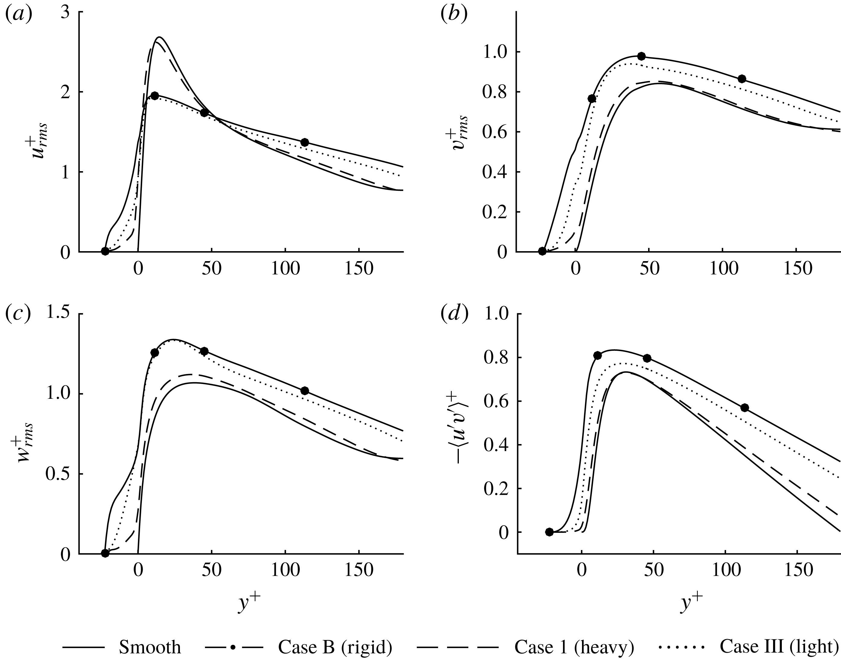
Figure 11. Profiles of (a) streamwise (b) wall-normal and (c) spanwise r.m.s. velocity, together with the Reynolds shear stress (d). Scaling is based on $u_{\unicode[STIX]{x1D70F}}^{f}$ . The filaments of cases B and III result in an increased isotropy by decreasing the streamwise component, while increasing the wall-normal and spanwise components.

4.2.2 Turbulent fluctuations

Figure 12. Wall-normal velocity fluctuations, $v^{+}$ , at the crest plane of the filaments, $y=0$ , for (a) case I and (b) case III, at one instant. Scaling is based on $u_{\unicode[STIX]{x1D70F}}^{f}$ . The velocity field of I contains relatively isolated sweep events, whereas strong velocity fluctuations are much more frequent for III.

In order to understand in more detail how the flow inside the bed interacts with turbulence just above the bed, we present the turbulent fluctuations scaled with local values of the friction velocity, $u_{\unicode[STIX]{x1D70F}}^{f}$ . R.m.s. velocities and the Reynolds shear stress (RSS) at the filament wall are presented in figure 11. Let us first characterise the fluctuations above the bed ( $y>0$ ). For all three normal components and the RSS, case I (dashed lines) shows only small deviations from the smooth wall profiles (solid lines). We can conclude that case I is not only slow, making it act as a rigid rough wall, but it is also so dense that it acts as a smooth wall. The turbulence–surface interaction of case I is thus essentially one-way coupled, i.e. surface deforms slowly due to streaks (figure 7 a), but the flow is essentially left unmodified by the surface.

In contrast, for case III, one observes that above the bed, the streamwise velocity component (dotted line in figure 11 a) is prominently reduced, whereas the wall-normal and spanwise components (figure 11 b,c) are increased. The rigid case B (filled circle symbols) behaves similarly. The decrease of the peak of the streamwise component can be attributed to the reduction (or even absence) of streaks. The increase of the peak values of the wall-normal and spanwise components can be attributed to disturbances caused by the filamentous wall, in particular to ejections from the interior of the bed, similarly as observed for rough walls by Orlandi & Leonardi (Reference Orlandi and Leonardi2006). The wall-normal velocity field at one instant is shown in figure 12 for I and III at the crest plane of the filaments, $y=0$ . The character of the velocity fields reflect those of the displacement fields, figure 7, with a high isotropy for III.

The strong interaction with the fast filamentous wall of case III is related to a reduction of the so-called wall-blocking effect, commonly observed for highly permeable walls (Breugem et al. Reference Breugem, Boersma and Uittenbogaard2006). Wall blocking occurs as fluid moving towards the wall cannot penetrate the wall and must change direction to move parallel to a wall, creating a ‘splat’ event (Perot & Moin Reference Perot and Moin1995). Energy is transferred from the wall-normal component to the tangential components, increasing tangential turbulence intensity.

For case III, which shows local regions of higher permeability, the fluid moving towards the wall penetrates the filamentous bed. This can be observed in figure 11(b), where $v_{rms}^{+}$ is relatively large for $y<0$ . As a consequence, velocity fluctuations are transported into the bed, inducing larger $u_{rms}^{+}$ and $w_{rms}^{+}$ between the filaments. The RSS, figure 11(d), confirms this by also having large values for $y<0$ . Note that the r.m.s. wall-parallel displacements, $(\tilde{q}_{x},\tilde{q}_{z})_{rms}$ , are smaller for the fast bed (III) compared to the slow bed (case I). The velocity fluctuations inside the fast bed show the reverse trend: velocity r.m.s. are larger in case III than case I. This indicates that the fluctuations inside the interior of the bed, are not primarily due to movement of the filaments, but rather due to penetration and ejections of turbulent fluctuations (similar to as rough wall).

5.1 A lumped-spring model of the surface

In this section, we analyse the filament time scale more quantitatively by formulating a transfer function representing the filaments. With a quasi-static assumption, it is possible to form a transfer function using the Euler–Bernoulli equation (Brücker, Bauer & Chaves Reference Brücker, Bauer and Chaves2007). The spatial shape of the filaments is then assumed to be the same in the static and the dynamic case. The resulting equation describes a damped harmonic oscillator, and the model can therefore be seen as a lumped-spring model of the filament dynamics. Analytical results are presented below, but the detailed derivation is provided in appendix A.

The transfer function in the streamwise direction, giving the tip deflection amplitude $\hat{q}_{x}(\unicode[STIX]{x1D714})$ from the tip force $\hat{F}_{tip}(\unicode[STIX]{x1D714})$ , as function of the angular frequency $\unicode[STIX]{x1D714}$ , is

(5.1) $$\begin{eqnarray}|H(\unicode[STIX]{x1D714})|=\frac{1}{\sqrt{\left(1-\left({\displaystyle \frac{\unicode[STIX]{x1D714}}{\unicode[STIX]{x1D714}_{n}^{LSM}}}\right)^{2}\right)^{2}+4\unicode[STIX]{x1D701}^{2}\left({\displaystyle \frac{\unicode[STIX]{x1D714}}{\unicode[STIX]{x1D714}_{n}^{LSM}}}\right)^{2}}},\end{eqnarray}$$

normalised with the mean displacement

(5.2) $$\begin{eqnarray}\langle \tilde{q}\rangle =\frac{1}{3}\frac{\langle F_{tip}\rangle l^{3}}{EI}\end{eqnarray}$$

so that $|H(0)|=1$ . In the lumped-spring model (LSM), the natural frequency is

(5.3) $$\begin{eqnarray}\unicode[STIX]{x1D714}_{n}^{LSM}=2\unicode[STIX]{x03C0}f_{n}^{LSM}=\frac{2}{l^{2}}\sqrt{\frac{2EI}{A\unicode[STIX]{x1D70C}_{s}+\unicode[STIX]{x1D712}}},\end{eqnarray}$$

and the damping ratio is

(5.4) $$\begin{eqnarray}\unicode[STIX]{x1D701}=\langle \tilde{q}\rangle \unicode[STIX]{x1D714}_{n}^{LSM}\left[\frac{c}{2\langle F_{tip}\rangle }\right],\end{eqnarray}$$

where $\langle F_{tip}\rangle =\hat{F}_{tip}(0)$ is the mean force on a filament. Here, $c$ is a damping constant, defined in appendix A, that depends only on the geometry. Equation (5.2), together with (2.7), show that $Q^{\ast }=3\langle \tilde{q}\rangle /a$ , and (5.3) resemble the natural frequency, equation (2.8), but with a slightly different coefficient.

The fraction in the brackets in expression (5.4) depends, to a first approximation, only on the geometry, so that for a given bed $\unicode[STIX]{x1D701}$ scales with the product of the resonance frequency and the mean amplitude, $\langle \tilde{q}\rangle \unicode[STIX]{x1D714}_{n}^{LSM}$ . This is reasonable since $\langle \tilde{q}\rangle \unicode[STIX]{x1D714}_{n}^{LSM}$ is a characteristic speed of the filaments. When inertia dominates over viscous damping ( $\unicode[STIX]{x1D701}<1/\sqrt{2}$ ), $|H|$ is fairly constant for $f<f_{n}^{LSM}$ , with a slight bump at, or close to, $f_{n}^{LSM}$ , after which it decreases. In this sense, it corresponds to a low pass filter, apparent from figure 6(d,e). A similar transfer function is present in the spanwise direction; the filament geometry is isotropic except for the reconfiguration induced by the mean displacement.

Note that there exist other surface time scales; if instead inertia is neglected, $A\unicode[STIX]{x1D70C}_{s}+\unicode[STIX]{x1D712}$ is assumed to small and hence the natural frequency, $\unicode[STIX]{x1D714}_{n}^{LSM}$ , is large. A new time scale then determines the response in (5.1),

(5.5) $$\begin{eqnarray}T=4\unicode[STIX]{x03C0}\frac{\unicode[STIX]{x1D701}}{\unicode[STIX]{x1D714}_{n}^{LSM}}=2\unicode[STIX]{x03C0}\frac{cl^{3}}{6EI},\end{eqnarray}$$

which is independent of the density of the filaments. This is the time scale in the viscous regime, determining the cutoff frequency of the filaments when damping dominates. For example, this is the case of more sparsely placed sensor filaments (Brücker et al. Reference Brücker, Bauer and Chaves2007). It is also similar to the poroelastic time scale discussed by Skotheim & Mahadevan (Reference Skotheim and Mahadevan2004, Reference Skotheim and Mahadevan2005). The latter time scale determines how fast the pressure (and thus the flow) inside a poroelastic medium equilibrate to the far field conditions. The speed of which the surface equilibrates to the surrounding is thus set by fluid transport, rather than by the deformation of the filaments.

5.2 Beds with higher resonance peak or smaller mean displacements

Next, we will compare the analytical predictions of the transfer functions from previous subsection with the transfer functions computed from numerical simulations (appendix B).

In addition to cases I and III, studied in depth in § 4, figure 13(a–c), also shows the transfer function for case II. Configuration II has filaments with resonance frequency ( $f_{n}^{+}=0.024$ ) in between I and III, and one may expect that the filaments will yield to forces of higher frequencies than in case I ( $f_{n}^{+}=0.0080$ ), but not as high as in III ( $f_{n}^{+}=0.057$ ). By comparing figures 13(b) and 13(c), we observe that case II has a significantly higher resonance peak than III. This means that displacements at this frequency are higher for the same imposed force. This is reflected by the r.m.s. values of the displacements, which are significantly larger for II than III,

(5.6) $$\begin{eqnarray}\left.\begin{array}{@{}c@{}}(\tilde{q}_{x},\tilde{q}_{z})_{rms}=(2.10,2.53)a\quad \text{for II and}\\ (\tilde{q}_{x},\tilde{q}_{z})_{rms}=(0.90,0.87)a\quad \text{for III}.\end{array}\right\}\end{eqnarray}$$

As a result of the resonant behaviour, above the bed ( $y>0$ ), the velocity fluctuations in all three directions are enhanced. In particular, we observed that the peak value of the spanwise r.m.s. velocity, $w_{rms}^{+}$ , is larger by 20 % and the wall-normal, $v_{rms}^{+}$ , by 5 %. However, higher resonance of the surface does not result in a larger entrainment into the bed. At the filaments tips $(y=0)$ , $v_{rms}^{+}$ is lower by 31 % (comparing II to III); this indicates that even though case II has significantly larger filament displacements than case III, it corresponds to a surface of lower apparent permeability than III. It thus seems that due to the high resonance peak, the filaments respond stronger to the turbulent flow. However, the lower resonance frequency and the higher resonance peak of the surface compared to III inhibit the surface to comply to sweep events to the same extent.

Figure 13. Absolute value of measured transfer functions between $F_{tip}$ and $\tilde{q}_{x}$ for cases I–VI in (a–f), respectively. Predicted transfer functions are also shown, calculated by (5.1).

The corresponding analytical predictions of the transfer functions of the filaments (obtained from (5.1)) are shown with a dashed line in figure 13(a–c) for cases I–III, with added mass according to (2.3). The parameter $c$ in (5.4) is fixed to one value ( $c=5.9~\unicode[STIX]{x03BC}\text{l}$ ) for all the transfer functions shown in figure 13, chosen by fitting the data. This value gives damping ratios in the interval $0.02\leqslant \unicode[STIX]{x1D701}\leqslant 0.4$ . We observe that the model predicts the response behaviour of the surface reasonably well. The model is empirical in the sense that it requires estimates of lumped parameters that depend on the fluid and flow properties, i.e. added mass $\unicode[STIX]{x1D712}$ and damping coefficient  $c$ .

We performed three additional simulations (with same fixed $c$ and $\unicode[STIX]{x1D712}$ as before), namely cases IV–VI in table 1. Compared to cases I–III, these configurations have a lower predicted mean displacement but the same predicted resonance frequencies. In this way, we can assess whether the fluid–surface interaction for heavier but stiffer beds also is determined by $f_{n}^{+}$ alone. The transfer function of these configurations are shown in figure 13(d–f) and table 4 reports the drag and the r.m.s. displacements. We note that these configurations behave very similarly to I–III; (i) the case with lowest natural frequency, IV, has a drag close to that of A ( $\unicode[STIX]{x0394}D=0.03$ and $\unicode[STIX]{x0394}D=0.02$ respectively), whereas the drag is much higher for V and VI ( $\unicode[STIX]{x0394}D=0.34$ and $\unicode[STIX]{x0394}D=0.37$ ); (ii) case IV also has a lower isotropy of the flow velocity than V and VI, apparent from the displacement r.m.s. values.

This parametric study demonstrates that both the model and the simulations show a consistent behaviour when it comes to bed response to turbulent forcing. In other words, the fluid–surface interaction is indeed determined by resonance frequency only, and one may either change the mass of the filaments or their elasticity to tune the response.

From figure 13, we observe for all cases that the frequency of the resonance peak is over-predicted by the model. This is also observed in figure 6(c,f). Looking at the expression for the location of the natural frequency, equation (5.3), this appears to be related to an underprediction of $\unicode[STIX]{x1D712}$ . Possibly, the modelling of the filament–filament coupling by $\unicode[STIX]{x1D712}=\unicode[STIX]{x1D70C}s^{2}$ (2.3) can be improved, although this very simple model suffices to capture the fluid–structure interaction and to provide physical insight.