2.1. Experimental apparatus

The experiments were performed in the Mach 6 hypersonic wind tunnel at Peking University (Zhu et al. Reference Zhu, Lee, Chen, Wu, Chen and Gad-el-Hak2018). The tunnel is a blow-down hypersonic facility, which can provide Mach 6 air flow through a relatively short axisymmetric nozzle, with a 160 mm exit diameter and open-jet test section. The continuous operation time can be as long as 30 s. This tunnel can be operated as a conventional one with the bleed valve closed. For the noisy flow, the r.m.s. pressure fluctuation is approximately 2.20 %. High-quality glass windows of 200 mm diameter provide optical measurement access. To avoid liquefying the air, the flow is pre-heated to a nominal stagnation temperature of 430 K by means of an electric heater. The model used was based on our previous work with slight modifications (Si et al. Reference Si, Huang, Zhu, Chen and Lee2019), as shown schematically in figure 1. The model is a flared cone of total length 260 mm. The boundary-layer thickness on the model surface of the flared section remains almost constant in the flow direction, so that the most amplified second mode (wavelength is approximately twice the boundary-layer thickness) grows significantly. Its geometry consists of a $5^{\circ }$ half-angle circular conical profile for the first 100 mm of axial distance, followed by a tangent flare of radius 931 mm until the base of the cone at the 260 mm axial position. In the experiments, the model is divided into three parts. The first 50 mm of the model is made of stainless steel. The middle 110 mm of the model, which can be replaced by a wavy wall, is made of polyether ether ketone (PEEK). The last 100 mm long part is a shell made of PEEK. The r.m.s. surface roughness of the PEEK shell is less than $0.2\,\mathrm {\mu }$m. Different model components are connected together by threads, and the cone is installed along the centreline of the nozzle with zero angle of attack. The length of the flow field that is not affected by the reflected Mach waves is more than 400 mm, which is long enough to embed the whole length of the model.

Figure 1. Sketch of the flared-cone model with a wavy wall. (a) Schematic of the model and the body-oriented coordinate. The blue area represents the streamwise range of experimental measurements. (b) Scheme of the wavy surface. (c) Photo of the model. (d) Model installation in wind tunnel test section.

For the present study, the region of the grooved wavy wall comprises 20 round arc cavities. The streamwise length of each cavity is 3 mm. The streamwise length of each cavity is close to the wavelength of the typical second mode. The depth of the cavity, $d=1$ mm, is approximately equal to the boundary-layer thickness $\delta$ (where $\delta \approx 0.95$ mm at $x=100$ mm). The wavy wall initiates at 100 mm downstream of the cone tip. The centre of the flared section of the model is at $(x_0,y_0)$. The shape of the wavy wall is obtained from the superposition of small arc cavities (magenta line in figure 1), and the start and end points of these arc cavities are distributed on the arc with radius $R$ (solid red line) and the arc with radius $R+d$ (dashed red line), as shown in figure 1(b). The central angle corresponding to half of the cavity is $\theta$. The radius of the arc cavities is determined by the formulas

(2.1)\begin{gather} \theta =\arcsin \left( \frac{w}{2( R+d )} \right), \end{gather}

(2.2)\begin{gather} {{d}_{1}}=\sqrt{{{( R+d )}^{2}}-{{\left( \frac{w}{2} \right)}^{2}}}-R, \end{gather}

(2.3)\begin{gather} \frac{{{d}_{1}}}{\sqrt{{{d}^{2}}+{{\left( \dfrac{w}{2} \right)}^{2}}}}=\dfrac{\sqrt{{{d}^{2}}+{{\left( \dfrac{w}{2} \right)}^{2}}}}{2r}, \end{gather}

where $R=931$ mm, $d=1$ mm and $w=3$ mm. At the joint of the cavities, small circular arcs are used to make smooth connections.

2.2. Focused laser differential interferometry

Focused laser differential interferometry (FLDI) measures the fluctuations in a hypersonic boundary layer based on the principle of optics, and has the advantages of high dynamic response, high spatial resolution, and high signal-to-noise ratio. Most importantly, as a non-contact optical measurement method, FLDI can provide information on the development of disturbances within the wavy zone, where surface pressure sensors cannot be used. Recently, Xiong et al. (Reference Xiong, Yu, Lin, Zhao and Wu2020) used FLDI to conduct a stability experiment for the boundary layer in a hypersonic wind tunnel of Mach 6. The results showed that FLDI captured successfully the second-mode instability wave and its harmonic wave.

A sketch of the FLDI setup is given in figure 2(a), and the overall optical system is symmetrical. First, a laser emits coherent light as the light source, and a concave lens (C1) diverges the laser beam through a polarizer (P1) and a Wollaston prism (W1) before it reaches the convex lens (C2). A commercial helium–neon laser was used as the light source, which emits polarized light with wavelength 632 nm. The focal lengths of the concave lens C1 and the convex lens C2 are 30 mm and 200 mm, respectively. The Wollaston prism has a small separation angle of 2 arc min. As the divergent laser beam passes through the Wollaston prism, the single beam is separated into two orthogonally polarized beams with a slight divergence angle. These two separated beams are converged using a convex lens (C2). Due to the slight divergence angle of the Wollaston prism, these two orthogonally polarized beams will be separated by a fixed distance at the focal point, shown as $\Delta X$ in the expanded portion of figure 2(a). The separation distance at the FLDI focus is less than 0.1 mm if the centre of the rhombus region is taken as the measurement point. Before these two orthogonally polarized beams converge to the focal point, they share almost the same optical path; thus no phase difference is assumed to be introduced if there was no inhomogeneity along their paths. At the focal point, the two beams are converged and do not share the same optical path, as seen from the sensitive length $L$ in figure 2(a). This small volume is defined as the probe of the FLDI system. Thus any inhomogeneity of the flow within this range will produce an optical path length (OPL) difference, as expressed by

(2.4)\begin{equation} \Delta {\rm OPL}=(n_1-n_2)L=\Delta n L, \end{equation}

where $n_1$ and $n_2$ are the refractive indices of the air at the two focal points, and $L$ is the sensitive length indicated in figure 2(a). Due to such an OPL difference, the phase difference $\Delta \phi$ of these two orthogonally polarized beams is

(2.5)\begin{equation} \Delta \phi=\frac{2 {\rm \pi}}{\lambda_0}\,\Delta {\rm OPL}, \end{equation}

where $\lambda _0$ is the wavelength of the laser (632 nm). Substituting the Gladstone–Dale relationship into (2.5), the phase difference can be expressed as

(2.6)\begin{equation} \Delta \phi=\frac{2 {\rm \pi}}{\lambda_0}\,LK(\rho_1-\rho_2)=\frac{2 {\rm \pi}}{\lambda_0}\,LK\,\Delta \rho, \end{equation}

where $K$ is the Gladstone–Dale constant ($0.0002257\,{\rm m}^3\,{\rm kg}^{-1}$ for air), and $\rho$ is the density. So the density of the flow is associated with the phase difference. Beyond the focal point, the beams are reconverged by the C3 lens. Another Wollaston prism (W2) and polarizer (P2) will recombine the orthogonally polarized beams, and finally the recombined beam will be registered as irradiance by the photodetector (D). Assume that $I_1$ and $I_2$ are the irradiances of the two orthogonally polarized beams, $l_1 \boldsymbol {\cdot } l_2$ is the unit vector's dot product of the beams, and the resultant irradiance at the photodetector surface is

(2.7)\begin{equation} I_d=I_1+I_2+2 l_1 \boldsymbol{\cdot} l_2 \sqrt{I_1 I_2}\cos(\Delta \phi). \end{equation}

Figure 2. (a) Sketch of the FLDI set-up: C1 – 30 mm divergent lens; C2 and C3 – 200 mm focal lenses; P1 and P2 – polarizers; W1 and W2 – Wollaston prisms (2 arc min); A – probe volume; and D – photodetector; $L1=300$ mm, $L2=600$ mm, $L3=200$ mm; the zoomed-in area displays the FLDI optical path length (OPL). (b) Laser emission side of the FLDI set-up. (c) Laser receiving side of the FLDI set-up.

By replacing the irradiance to the potential response of the photodetector, the relationship between density fluctuation and output voltage of system is established as

(2.8)\begin{equation} \Delta \rho=\frac{\lambda_0}{2 {\rm \pi}LK}\sin^{{-}1}\left(\frac{V}{V_0}-1\right), \end{equation}

where $V$ is the potential response of the photodetector, and it can be expressed by ${V=I_dRR_L}$, in which $R$ denotes the responsivity of the photodiode, and $R_L$ is the load resistance. Also, $V_0$ corresponds to the most linear part of a fringe before each experiment, and it can be expressed by $V_0=2I_0RR_L$.

In this research, the time trace signals of the FLDI system are acquired with a Spectrum M2i.4652 transient recorder. The signal is stored in a 16-bit format. The sampling rate of the transient recorder is chosen as 3 MHz for the current experiment to resolve the ultra-high-frequency harmonic instabilities. FLDI is a single-point measurement system. The information at one position is recorded for each run. Under the same experimental conditions, the measurements are repeated many times to obtain the entire disturbance evolution in the flow direction.

2.3. Direct numerical simulations

In this subsection, we introduce briefly the model and numerical settings for the direct numerical simulations (DNS). The parallel CFD software OPENCFD, developed by Li, Fu & Ma (Reference Li, Fu and Ma2008), was used for the DNS. Jacobian-transformed compressible Navier–Stokes equations in curved coordinates are solved numerically using high-order finite-difference methods. An accurate shock-fitting finite-difference method based on the fifth-order upwind compact scheme was employed to discretize inviscid flux derivatives of the governing equations. Meanwhile, a sixth-order central-difference scheme was used to discretize viscous terms. A third-order total variation diminishing (TVD) type Runge–Kutta method is used for the time stepping. The fluid is assumed to be a perfect gas with specific heat ratio $\gamma =1.4$ and Prandtl number $Pr=0.72$. The dynamic viscosity $\mu$ is calculated using Sutherland's formula $\mu =\mu _{\infty } {\bar T}^{3/2}({\bar S}+1)/({\bar S}+{\bar T)}$, where ${\bar T}=T/T_{\infty }$ is the dimensionless temperature, and ${\bar S=110.4\ K/T_{\infty }}$. This code parallelized using the MPI library has been applied successfully to simulate other hypersonic boundary-layer stability problems (Li et al. Reference Li, Fu and Ma2008; Li, Fu & Ma Reference Li, Fu and Ma2010).

Computations consist of two steps. In the first step, steady flow is computed with the computational domain covering the cone head and the bow shock. In the second step, the transition flow in the boundary layer is computed with the computational domain inside the bow shock that does not contain the cone head. The flow conditions correspond to freestream Mach number 6.0, freestream pressure ($p_e$) 570 Pa, freestream temperature ($T_e$) 50.89 K, and unit Reynolds number ($Re_{\infty }$) $9.3 \times 10^6\,{\rm m}^{-1}$. No-slip and adiabatic conditions are prescribed at the wall. In our computation, the nose radius was set to $r_n=0.1$ mm, as listed in table 1. In the present case, the roughness patch is modelled using a body-fitted grid. Figure 3(a) shows a sketch of the computational grid, with an expanded view of the part near the wavy wall in figure 3(b). A mesh consisting of 5000 and 200 grid points in the streamwise and wall-normal directions is used for the simulation.

Table 1. Freestream conditions for the experimental study and numerical simulation.

Figure 3. Computational grid of the domain: (a) schematic of grid for simulations; (b) close-up of the restricted domain.

For the two-dimensional case, the wall-normal velocity component at the wall is specified in the primary blowing–suction strip region as

(2.9)\begin{equation} v_{bs}(x,0,z,t)=A_0(2 \epsilon-1),\quad x_1 \le x \le x_2, \end{equation}

where $\epsilon$ is a random number generated by the system, between 0 and 1, and $A_0$ is the amplitude level of the random perturbations. The variables $x_1$ and $x_2$ indicate the boundaries of the strip ($x_1=20$ mm, $x_2=25$ mm). Here, $A_0$ is set to be $1.0 \times 10^{-6}$ to obtain the linear evolution of disturbances. A similar method was used to simulate natural transition in boundary layers via random inflow disturbances (Hader & Fasel Reference Hader and Fasel2018; Lugrin et al. Reference Lugrin, Beneddine, Leclercq, Garnier and Bur2021). In the present work, it was chosen not to decide which instability was going to be dominant and to let all of them compete in the simulation. For the present study, the length scale is non-dimensionalized by a specific length $L^{*}$, and the dimensionless time $t$ is obtained through $t=L^{*}/U_{\infty }^{*}$. Here, $L^{*}=1$ mm, and $U_{\infty }^{*}$ is the velocity of the freestream.

2.4. Method description of Lagrangian tracking

The datasets from DNS are used to reconstruct the evolution of flow structures by employing the method of Lagrangian tracking of marked particles. A particle pathline shows the sequence of particle locations over time as a particle moves through a fluid medium. If a grid of particles is traced, then the evolution of a material surface that is comprised of the particles can be obtained. A streakline provides a more intuitive physical view than a pathline, because it consists of a series of fluid particles that are repeatedly released from a fixed location. Timelines are lines connecting a series of particles released from different locations at the same time.

It is known that applying Lagrangian tracking on a fluid element forms a trajectory of the particle. This is completed by integrating an ordinary differential equation (ODE):

(2.10)\begin{equation} V(X(t),t)={\rm d}X(t)/{\rm d}t. \end{equation}

Here, $V(X,t)$ is an unsteady velocity field obtained from particle image velocimetry or DNS over a finite time interval $[t_0,t_1 ]$. When extracting the evolution of a material domain, Lagrangian tracking is applied on a specific space domain

(2.11)\begin{equation} X_0 \to X, \end{equation}

where $X_0$ is the region of interest at $t_0$ from where the Lagrangian tracing is applied. And the obtained new position $X(t)$ is the material region evolving from $X_0$, with $t \in [t_0,t_1 ]$, during which the velocity field $V(X,t)$ is interpolated at each step according to the new position of $X(t)$. If the initial space domain $X_0$ is a particle, then a trajectory will be generated. And if $X_0$ is a flat surface, then the evolution of the specific material surface is obtained. In the present study, this is achieved using a MATLAB algorithm that employs an ODE solver and interpolation scheme. The Dormand–Prince method (ode45 in MATLAB) is chosen as the solver for trajectory advection, and the absolute and relative tolerances of the ODE solver were set at $10^{-6}$. Here, absolute error tolerance is a threshold below which the value of the solution becomes unimportant. Relative error tolerance measures the error relative to the magnitude of each solution component. Equation (2.10) is integrated over a time interval $[t_0,t_1 ]$, for a specified initial condition.

3.1. Base flow field

Figure 5(a) shows the streamwise development of the boundary-layer thickness and wall pressure for the smooth and wavy walls. The edge of the boundary layer is determined as the point at which the velocity exceeds $0.95U_{\infty }$. It is observed that the wall curvature causes a reduction of the boundary-layer thickness in the flared portion of the cone. As a result, the flow near the boundary layer moves towards the wall, which induces a significant pressure increase. The boundary-layer thickness and wall pressure on the wavy wall are consistent with that of the smooth wall, until the wavy region is reached. The boundary-layer thickness and wall pressure vary periodically in the streamwise direction, and are highly correlated with the wavelength of the waviness. The favourable pressure gradient zone and the adverse pressure gradient zone appear alternately. The presence of waviness also affects the mean flow downstream of the wavy region. In the downstream limit, the velocity field tends to recover to the unperturbed state, as shown in figure 5(b).

Figure 5. Characteristics of the mean flow: (a) boundary-layer thickness and wall pressure; (b) normalized streamwise velocity and temperature profiles at $x=165$ mm. The dashed lines represent the smooth wall, and the solid lines represent the wavy wall.

A representation of the flow field is shown in figure 6 as density gradient contours. The single wavy roughness causes a compression followed by an expansion, which appears within the wavy region. This alternating compression/expansion is actually similar to the case described by Marxen, Iaccarino & Shaqfeh (Reference Marxen, Iaccarino and Shaqfeh2010). There is a significant change in the smooth part starting approximately 0.5 mm from the surface for the density gradient in the normal direction, as shown in figure 6. Within the wavy region, a series of compression waves is visible above the wavy troughs, and the compression waves are at an angle of approximately $11.5^{\circ }$ to the direction of flow.

Figure 6. Contours of the absolute wall-normal density gradient $|{\partial \rho }/{\partial y}|$ for the wavy wall.

The 14th wavy segment, located between $x=139$ mm and $x=142$ mm, is selected as the reference case and discussed in detail. Figure 7 shows the velocity vectors of the flow field in this region. The velocity in the near-wall region is approximately linearly distributed on the smooth wall, which is a typical feature of a hypersonic boundary layer (Pruett & Chang Reference Pruett and Chang1998). In contrast, the velocity profile is somewhat concave on the wavy wall, especially above the trough. To show the characteristics of the flow field in the wavy region more clearly, the velocity and temperature profiles of six locations near the 14th segment are shown in figure 8. All profiles at the different positions in the local region for the smooth wall are essentially identical. However, the velocity and temperature profiles for the wavy wall change significantly and deviate significantly from the smooth wall. This has two effects on the mean flow: first, a shear layer develops along the trough segment, which is absent for the smooth wall; second, affected by the spatially modulated mean flow, the positions of the relative sonic line and the inflection point of the boundary-layer profile may deviate significantly from the smooth condition. These effects have an important impact on the development of the first and second modes in the hypersonic boundary layer. New instabilities may arise due to the mean-flow distortion caused by the wavy wall.

Figure 7. The velocity vectors of the base flow: (a) smooth wall, (b) wavy wall. The coordinates of the six selected points are: point 1, $x=142.16$ mm; point 2, $x=142.77$ mm; point 3, $x=143.51$ mm; point 4, $x=143.70$ mm; point 5, $x=144.23$ mm; point 6, $x=145.62$ mm;

Figure 8. The velocity (magenta) and temperature (blue) profiles at the six selected locations in figure 7 for the smooth and wavy walls: (a) point 1, (b) point 2, (c) point 3, (d) point 4, (e) point 5, ( f) point 6. Here, the dashed lines represent the smooth wall, and the solid lines represent the wavy wall.

3.2. Disturbance frequency spectra

First, the evolution of the disturbance amplitude along the surface of the flared cone is analysed. These frequency spectra, from both experimental measurements of FLDI and numerical simulations, are similar to the results obtained using high-frequency pressure sensors in early experiments (Zhu et al. Reference Zhu, Lee, Chen, Wu, Chen and Gad-el-Hak2018), as shown in figure 9. In the experiment, high-frequency density signals are collected and recorded using the FLDI system, which can analyse the amplitude evolution of disturbances at different frequencies. This non-contact optical approach allows for measurements in the vicinity of the wavy surface, and provides more information than previous experiments using wall-mounted pressure sensors (Si et al. Reference Si, Huang, Zhu, Chen and Lee2019). In the absence of knowledge about the types of disturbances on the wavy wall, assessment of the frequency spectra can help to determine the disturbance components. Figure 9(a) illustrates the power spectral densities (PSDs) of instability waves in the flow direction. These sampling points are located approximately $0.6 \pm 0.15$ mm from the model surface, from $x=90$ mm to $x=181$ mm downstream from the cone tip. At the most upstream measurement position, $x=90$ mm, only a very low-frequency peak appears, and no other instability waves are observed, with electronic noise prominent at the high-frequency domain. As the flow moves downstream, the disturbances at other frequencies gradually develop. The frequency spectra at sampling positions exhibit two additional peaks for the smooth wall, except for low-frequency waves. The significant frequency peak at $f\approx 360$ kHz indicates that the second mode grows on the smooth wall. Another peak at $f\approx 720$ kHz corresponds to the harmonic of the second mode, which was also observed in the experiment of Zhu et al. (Reference Zhu, Lee, Chen, Wu, Chen and Gad-el-Hak2018).

Figure 9. Comparison of disturbance frequency spectra obtained by experiment and calculation for the smooth wall and the wavy wall. (a) Power spectral density (PSD) comparison of FLDI. The measurement locations are located in the blue area in figure 1(a). (b) Amplitude spectra of calculated results. Black lines are for the smooth wall, and red lines are for the wavy wall.

For the wavy wall, there are two additional peaks in the frequency spectra. The frequency peak corresponding to the second mode on the smooth wall is still significant on the wavy wall, but is attenuated in the wavy zone ($x=100$ mm to $x=160$ mm) and grows rapidly again downstream. The frequency of this peak in the experiments, $f\approx 380$ kHz, is slightly higher than the second mode on the smooth wall. For the wavy wall, two new peaks centred at $f\approx 140$ kHz and $f\approx 260$ kHz appear in the frequency spectra, absent in the upstream smooth part, and appear to be related to the distortion due to the wavy troughs. In the wavy region, these two frequency peaks appear, and the power spectral density values exceed the value of the peak of the second mode. The experimental measurements obtained by FLDI can be verified by PCB fast response pressure sensors, which are used commonly in hypersonic wind tunnels. In the experiment, the sensor was located at $x=173$ mm. The frequency spectra at two different unit Reynolds numbers are shown in figure 10. It can be observed clearly that the second mode at $f=360$ kHz is suppressed by the wavy wall rather appreciably, with two additional peaks appearing in the frequency spectra for the wavy wall. These results agree well with the FLDI measurements. The amplitude spectra of maximum density disturbances in the wall-normal direction obtained from simulations are shown in figure 9(b). Both experiments and the DNS capture these two new frequency peaks. In the calculation, the disturbance is excited by low-amplitude blowing and suction, and evolves linearly. The amplitude of the low-frequency waves is very low, and the harmonics at $f\approx 720$ kHz related to the nonlinear interactions do not appear. The present research focuses on the physical mechanism of the enhancement of new instabilities, and the difference in the amplitudes of the low-frequency waves and the harmonic does not affect the conclusion.

Figure 10. Frequency spectra measured by PCB fast response pressure sensors at two different unit Reynolds numbers: (a) $Re_{\infty }=7.1 \times 10^6 \,{\rm m}^{-1}$; (b) $Re_{\infty }=9.3 \times 10^6 \,{\rm m}^{-1}$. Black lines are for the smooth wall, and red lines are for the wavy wall.

3.3. Disturbance evolution in the flow direction

In the previous subsection, the wavy wall is seen to modify the base flow. In light of results from Marxen et al. (Reference Marxen, Iaccarino and Shaqfeh2010) and Marxen, Iaccarino & Shaqfeh (Reference Marxen, Iaccarino and Shaqfeh2014), the two-dimensional roughness acts as an amplifier for two-dimensional convective disturbances within a certain frequency band, and the source of an additional perturbation. In this subsection, how disturbances are convected and amplified by the wavy wall is examined.

In order to show the spatial development of the disturbances in the boundary layer more clearly, bandpass filtering is performed on the time series signals collected using FLDI. The bandpass is centred at the three frequency peaks ($\,f=140$ kHz, $f=260$ kHz and $f=360$ kHz) in the spectra in figure 9, with bandwidth 20 kHz. The filtered density time series signals at nine streamwise positions on the smooth and wavy walls are shown in figure 11. The selected locations are distributed from $x=62$ mm to $x=213$ mm. On the smooth wall, it is observed that the disturbance at $f=360$ kHz grows more rapidly than other disturbances. On the wavy wall, the disturbances at $f=140$ kHz and $f=260$ kHz are enhanced within the wavy region ($x=100$ mm to $x=160$ mm). Compared with the smooth wall, the amplitude of these disturbances increases significantly. Downstream of the wavy region ($x>160$ mm), the disturbance at $f=360$ kHz amplifies rapidly.

Figure 11. Filtered density time series signals obtained from experimental measurements of FLDI at different streamwise locations: (a) $f=140$ kHz, (b) $f=260$ kHz, (c) $f=360$ kHz. In each panel, (i) indicates the smooth wall, (ii) indicates the wavy wall.

After Fourier transformation of the time series, the perturbation amplitude at a specific frequency is obtained. This approach is adopted to deal with the experimental measurement signals. The physical mechanism over a wavy wall can be illustrated further by considering the evolution of mode shapes with downstream distance. A carpet plot of the distribution of perturbation amplitude obtained by experimental FLDI measurements at various wall-normal locations for the smooth and wavy walls is shown in figure 12. In the flow direction, the mode shapes at $f=140$ kHz and $f=260$ kHz over the wavy wall get modified much more progressively than on the smooth wall, as shown in figures 12(a,b). This is consistent with the evolution of time signals in figure 11. However, the disturbances at $f=360$ kHz are more dramatic for the smooth wall.

Figure 12. Experimental measurements of disturbance amplitude at three frequencies for the smooth and wavy walls at $x_1=62$ mm, $x_2=106$ mm, $x_3=130$ mm, $x_4=148$ mm, $x_5=154$ mm, $x_6=165$ mm, $x_7=181$ mm and $x_8=197$ mm: (a) $f=140$ kHz, (b) $f=260$ kHz, (c) $f=360$ kHz. The black and red lines are for the smooth and wavy walls, respectively.

For the calculated results, the steady-state laminar flow field from DNS is used as a base flow, and is used in subsequent investigations to track the evolution of a small-amplitude perturbation. Here, 8000 two-dimensional flow fields with time interval 0.2 are saved, and processed similarly to the experimental dataset to obtain a flow field at a specific frequency. The contours of the pressure perturbations at $f=140$ kHz, $f=260$ kHz and $f=360$ kHz are shown in figure 13. The main part of the second mode at $f=360$ kHz on the smooth wall lies mainly near the wall, as shown in figure 13(a-i). Both the disturbance amplitudes at $f=140$ kHz and $f=260$ kHz, in figures 13(b-i) and 13(c-i), remain unchanged. Due to the modulation of the mean flow on the wavy wall, the disturbance at $f=360$ kHz in figure 13(a-ii) increases very slowly. By comparison, the disturbances at $f=140$ kHz and $f=260$ kHz, in figures 13(b-ii) and 13(c-ii), are amplified significantly within the wavy zone, with the wavy surface acting like an amplifier.

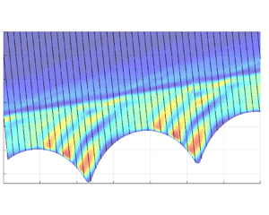
Figure 13. Amplitudes of the disturbances for three frequencies within the region $x \in [98\,{\rm mm}, 162\,{\rm mm}]$: (a) $f=140$ kHz, (b) $f=260$ kHz, (c) $f=360$ kHz. In each panel, (i) indicates the smooth wall, (ii) indicates the wavy wall.

Through numerical simulation analysis, an overall understanding of how the wavy trough alters the instability of the boundary layer is developed. In the simulation, a small-amplitude random perturbation is created by employing blowing and suction at the wall. The evolution of disturbances is analysed using a Fourier transformation. For two-dimensional axisymmetric disturbances, the evolution of the amplitudes of wall pressure disturbance in the flow direction for a wide range of frequencies is shown in figure 14. As is known, the dominant frequency of the second mode is closely related to the thickness of the boundary layer (Fedorov Reference Fedorov2011), and the variation trend is shown in figure 5(a). As the flow develops downstream, the boundary-layer thickness changes, and the disturbance's dominant frequency also shifts. As the boundary layer develops on the smooth wall, the frequency leading to the maximum amplitude transitions from approximately 350 kHz at $x=140$ mm to approximately 400 kHz at the end of the computational domain. By comparison, the disturbance amplitude at the same frequency for the wavy wall is lower. In addition, disturbances in the frequency range 120 kHz to 300 kHz are amplified significantly. The spatial growth rate ($-\alpha _i$) was calculated using a first-order accurate difference scheme of the natural logarithm of the pressure disturbance amplitude at the wall ($p'_{wall}$), and is expressed as

(3.1)\begin{equation} {(-\alpha_i)}_i=\frac{\ln(|p'_{i+1 | wall}|)-\ln(|p'_{i | wall}|)}{x'_{i+1 | wall}-x'_{i | wall}},\quad 2 \leq i \leq n_x, \end{equation}

where $i$ is the grid index in the streamwise direction. The comparison of contours of the spatial growth rate obtained by DNS for the smooth and wavy walls is shown in figure 15. For the smooth wall (figure 15a), at $x=160$ mm, the growth rate of the disturbances in the frequency range 350 kHz to 400 kHz increases significantly, while the growth rates of disturbances in other frequency ranges are much lower. For the wavy wall (figure 15b), the growth rate of the disturbance over a wide frequency range is modulated by the wavy surface in the range $x=100$ mm to $x=160$ mm. The alternating positive and negative changes in the growth rate indicate that the disturbance is periodically promoted and suppressed within the wavy region. And disturbances in the frequency range from 350 kHz to 400 kHz are greatly suppressed. Additionally, the growth rate of the disturbances between 120 kHz and 300 kHz is more pronounced within the wavy region.

Figure 14. The evolution of the amplitudes of wall pressure disturbance in the flow direction for a wide range of frequencies: (a) smooth wall, (b) wavy wall.

Figure 15. Contours of the spatial growth rate in the downstream direction for a wide range of frequencies: (a) smooth wall, (b) wavy wall.

3.4. Spatial distribution of disturbances

The evolution of the wall pressure disturbance amplitude at the three frequencies in the local wavy region is shown in figure 16(a), with an expanded view from $x=136$ mm to $x=144$ mm shown in figure 16(b). The red dashed lines bracket the change in disturbance amplitude over one surface wavelength. The amplitudes of these disturbances increase within the wavy region. Among these disturbances, the disturbance at $f=260$ kHz shows the fastest increase, followed by $f=140$ kHz, with the disturbance at $f=360$ kHz growing more slowly. Specific to one wavelength of the wavy trough, the disturbance amplitude increases with repeated jumps over the first half of the trough; over the second half of the trough, the disturbance amplitude decreases. Over the entire wavy zone, the amplitude exhibits exponential growth. In the experiments, the disturbance evolution at three frequencies within the 10th and 18th wavy troughs was measured in detail by FLDI, as shown in figure 17. Within each wave trough, the normal distribution of disturbance amplitudes at $x =X$ mm, $x=X+0.6$ mm, $x=X+1.0$ mm and $x=X+2.0$ mm was measured. Here, $X$ represents the starting position of the wavy trough. It is observed that the disturbance amplitude within the trough of $X=151$ mm is more significantly amplified than the disturbance amplitude within the trough of $X=139$ mm. Furthermore, the disturbance amplitudes at $x=X+2.0$ mm are much lower than disturbance amplitudes at $x=X+1.0$ mm. The experimental measurements are in qualitative agreement with the numerical simulations.

Figure 16. (a) The evolution of wall pressure disturbances on the wavy wall at the three frequencies in the flow direction. (b) An expanded view from $x=136$ mm to $x=144$ mm. (c) Sketch of one wavelength of wavy trough. The dashed lines bracket one wavelength of the wavy wall, as shown in the ellipse in (b).

Figure 17. Wall-normal distribution of disturbance amplitude at four stations within the wavy trough obtained through experimental measurements: (a) the 10th wavy trough, $X=139$ mm, (b) the 18th wavy trough, $X=151$ mm. In each panel: (i) $f=140$ kHz, (ii) $f=260$ kHz, (iii) $f=360$ kHz. Here, $A$ is the disturbance amplitude normalized by the maximum value.

The spatial distribution of velocity disturbances in the flow direction is shown in figure 18. For the smooth wall, the disturbance profile has two peaks, with the peak near the wall much more prominent, which is consistent with the results of previous research (Zhu et al. Reference Zhu, Lee, Chen, Wu, Chen and Gad-el-Hak2018). By comparison, the disturbances within the wavy trough display three or more peaks for the wavy wall. In previous studies (Nayfeh, Ragab & Al-Maaitah Reference Nayfeh, Ragab and Al-Maaitah1988; Dovgal, Kozlov & Michalke Reference Dovgal, Kozlov and Michalke1994; Diwan & Ramesh Reference Diwan and Ramesh2009; Xu et al. Reference Xu, Mughal, Gowree, Atkin and Sherwin2017) of a separation bubble for both incompressible flow and compressible flow at low Mach numbers, both experiments and calculations detected a third peak at the inflection point in the base flow profile. In research on roughness in hypersonic boundary layers, a disturbance with three maxima in the profile has also been observed by Marxen et al. (Reference Marxen, Iaccarino and Shaqfeh2010) and Zhao et al. (Reference Zhao, Dong and Yang2019). The origin of the third peak is thought by Diwan & Ramesh (Reference Diwan and Ramesh2009), Xu et al. (Reference Xu, Mughal, Gowree, Atkin and Sherwin2017) and Zhao et al. (Reference Zhao, Dong and Yang2019) to be an inflectional instability. For the smooth wall, periodic variations in the disturbance amplitude in the flow direction are observed in figures 18(a–c). Disturbances at different frequencies correspond to different wavelengths in the flow direction, which are easily distinguishable. The wavelengths of the disturbances at frequencies $f=140$ kHz, $f=260$ kHz and $f=360$ kHz are 3 mm, 2.1 mm and 1.6 mm, respectively. The situation is very different for the wavy case, as shown in figures 18(d–f). Within the wavy region, all perturbations are modulated by the wavy surface, and have wavelength 3 mm in the flow direction. The disturbance peaks on the smooth wall behave like bulges, while the disturbance peaks on the wavy wall behave like ridges, which are approximately perpendicular to the wall at an angle to the flow direction. These differences are more evident in the plan view, as shown in figure 19. The perturbation profiles at $f=140$ kHz, $f=260$ kHz and $f=360$ kHz for the wavy wall are approximately perpendicular to the curved wall and at a certain inclination angle to the freestream. There are one, two and three peaks in the first half of the wavy trough, respectively, implying that these disturbances at three different frequencies are affected by the mean-flow distortion due to the wall geometry, and their spatial distribution is modulated by the curved wall.

Figure 18. The spatial distribution of velocity disturbances of three frequencies in the flow direction: (a,d) 140 kHz, (b,e) 260 kHz, (c, f) 360 kHz. The amplitude of the disturbance is normalized by the maximum between $x= 139$ mm and $x= 145$ mm. (a,b,c) Smooth wall; (d,e, f) wavy wall.

Figure 19. Plan view of the velocity disturbances of three frequencies on the smooth and wavy walls: (a,d) 140 kHz, (b,e) 260 kHz, (c, f) 360 kHz. The amplitude of the disturbance is normalized by the maximum of the local location, and peaks are labelled with red numbers. (a,b,c) Smooth wall; (d,e, f) wavy wall.

3.5. Fluid movement pattern for the smooth and wavy walls

The present investigation attempts to understand the behaviour of fluid movement better by using a combination of both qualitative and quantitative techniques to assess fluid movement near the wall. The present study focuses on the difference between the movement of the mean flow on the smooth wall and the wavy wall in order to clarify the mechanism for disturbance growth. In this subsection, results are based primarily on marked particles, followed using Lagrangian tracking methods. Timelines are reconstructed from the datasets of the DNS velocity field. This Lagrangian approach provides good insight into the coherent structure evolution, and the current research is inspired by Zhao, Yang & Chen (Reference Zhao, Yang and Chen2016) and Haller et al. (Reference Haller, Hadjighasem, Farazmand and Huhn2016).

Figure 20 shows the normalized streamwise components of the base flow. The base flow displays similar profiles for the smooth wall within the selected region in the flow direction. For the wavy wall, a strong shear layer develops above the wavy trough, as indicated by the stretched timeline in figure 20(b). The change in the spacing of the velocity profiles in figure 20(b) indicates that the wavy surface induces periodic compression and expansion, with the fluid accelerating and decelerating periodically. The fluid behaviour corresponds to the previously observed periodic changes in pressure and density gradients above the wavy wall, as shown in figures 5 and 6. To clarify the difference in the fluid behaviour between the two different walls, the velocities on the smooth and wavy walls are shown in figures 20(c,d). The 20th grid point in the normal direction is selected as the observation object, and its spatial distribution is shown within the box. For the flow on the smooth wall, the streamwise velocity remains the same within the region $x=137$ mm to $x=141$ mm. However, modulated by the wavy surface, the change in the streamwise velocity on the wavy wall can reach 40$\%$ of the freestream velocity. At the peak of the trough, the velocity in the selected region ($x=137$ mm to $x=141$ mm) can reach almost half of the freestream velocity. It is expected that the wall-normal velocity near the wavy troughs is very significant. In the following sections, the details of fluid motion are explored with the help of timelines.

Figure 20. Normalized velocity profiles of base flow on (a) the smooth wall and (b) the wavy wall, and streamwise velocity on (c) the smooth wall and (d) the wavy wall. The regions outlined in red indicate the interface of the recirculation region, and the selected spatial positions of the flow field are shown in the box.

In order to generate timelines, the initial condition can be set as a fixed horizontal or vertical line, and the integration is implemented iteratively with an updating release time. Timeline patterns are formed by determining and displaying a sequence of timelines generated at a fixed frequency. Figure 21 shows a set of timelines to demonstrate the fluid behaviour around the wavy surface, and two snapshots on the smooth wall are used for comparison. Here, the reconstructed timelines are derived from the flow field calculated by the two-dimensional DNS. The initial condition is set as a fixed vertical line at $x= 140$ mm, and the integration is implemented iteratively with an updating release time. The instantaneous results are markedly similar to those shown using hydrogen bubble timelines of incompressible flow by Smith & Metzler (Reference Smith and Metzler1983).

Figure 21. (a) Side view of the evolution of the boundary layer based on timelines initiated at $x=140$ mm over the wavy wall: (i) $t=60.0$, (ii) $t=61.6$, (iii) $t=63.2$, (iv) $t=64.8$. The motion of the lower fluid is represented by fluid particles, and the upper side is replaced by lines. (b) Timelines initiated at $x=140$ mm and (c) timelines initiated at $x=164$ mm, on the smooth wall. Here, $\Delta y$ represents the relative value of the actual coordinates minus the coordinates of the smooth wall at the same streamwise position.

Figure 21(a) shows the evolution of timelines within the wavy region, and timelines at two streamwise positions on the smooth wall are shown in figures 21(b,c) for comparison. Since the timelines are released at a fixed frequency, the spacing of the timelines indicates the local acceleration and deceleration of the fluid, as the timelines are initially released at a fixed frequency. Modulated by the wavy geometry, the timelines on the wavy wall bend, rise and fall around the wavy surface. The timeline pattern shows that the flow accelerates at the top and decelerates at the bottom of the trough. In this process, the timelines will be stretched and deformed significantly, and a strong shear layer develops, as shown in figures 21(a) (i)–(iv). In general, the change of wall geometry introduces two kinds of motion to the mean flow: in the streamwise direction, the flow periodically accelerates and decelerates; in the normal direction, the flow moves up and down. For comparison, two sets of data on the smooth wall are selected. The timelines released at $x=140$ mm on the smooth wall are uniform, and no apparent fluctuations are observed. At $x=164$ mm, the timeline pattern at this position displays periodic compression and expansion caused by the typical second mode, with the flow structure appearing similar to the results of Zhu et al. (Reference Zhu, Lee, Chen, Wu, Chen and Gad-el-Hak2018).

In order to characterize the fluid behaviour in the wavy troughs, a velocity vector diagram within the recirculation region is shown in figure 22(a). The arrows represent the velocity vectors of the base flow, which show the rotation of the fluid, with the negative velocity component concentrated mainly in the second half of the trough. Five locations are selected within the trough to reconstruct the streaklines to illustrate the evolution of the flow within the recirculation region. At $Loc\,1$, the fluid velocity is initially fast at the top of the trough but decelerates as it enters the trough region. Figure 22(c) shows that the fluid at the top and the bottom moves in opposite directions at $Loc\,2$. The back and forth of the streaklines at the interface indicates that the fluid oscillates irregularly. The modulation of the mean flow can amplify a disturbance. It is within this region ($Loc\,2$) that disturbances are amplified, as shown in figure 16(b). Compared with the flow within the front half of the trough, the fluid within the second half of the trough moves downwards, with the fluid velocity faster than the entering fluid. Note that the fluid behaviour at $Loc\,5$ is similar to that at $Loc\,1$.

Figure 22. Evolution of streaklines initiated at different positions within the wavy zone: (a) velocity vector field in wavy trough; (b–f) correspond to the five locations in (a). The blue line in (a) represents the location of the smooth surface, and the blue arrows in (b–f) represent the movement directions of the streaklines.

4.1. Disturbance behaviours over a wavy wall

The wavenumber–frequency spectra, as described by Casper et al. (Reference Casper, Wagner, Beresh, Spillers, Henfling and Dechant2018), were utilized to determine whether upstream- and downstream-propagating disturbances exist simultaneously. This same approach was applied along the $x$–$y$ plane of the pressure disturbance signal using the fft2 command in MATLAB. The resulting wavenumber–frequency spectra are shown in figure 23. The slope of the line connecting these peaks gives the convection velocity of the disturbances. For the smooth wall, the most apparent peak appears at $(\,f,k_x)=(380,0.5)$, representing the disturbances at $f=380$ kHz with streamwise wavenumber 0.5. This peak corresponds to the downstream-propagating second mode. Compared with the smooth wall, the disturbances on the wavy wall occur over a wide frequency range from 50 kHz to 300 kHz. In figure 23(b), in addition to the peaks along the red line, which is similar to the case of the smooth wall, the perturbations of the same frequency can have multiple wavenumbers. For the newly amplified disturbances on the wavy wall, the frequency range is between 100 kHz and 300 kHz, and prominent peaks are observed on both sides of the wavenumber spectra, indicating that both upstream- and downstream-propagating disturbances exist simultaneously. This disturbance behaviour provides sufficient evidence for the existence of a flow mechanism similar to Casper et al. (Reference Casper, Wagner, Beresh, Spillers, Henfling and Dechant2018).

Figure 23. Wavenumber–frequency spectra of pressure fluctuations: (a) smooth wall, (b) wavy wall. PSD represents the power spectral density of the wavenumber–frequency spectra. The blue arrows point out the upstream-propagating perturbations.

The spatial distributions of amplitude spectrum and power spectrum provide a wealth of information about the properties along the wavy wall, as shown in figures 18 and 19. However, the dynamic behaviour of disturbances cannot be obtained through these time-invariant results. Sawaya et al. (Reference Sawaya, Sassanis, Yassir, Sescu and Visbal2018) pointed out that the wall deformations can transmit disturbance energy to the external flow, but the detailed process is unclear. Using a Morlet wavelet provided by Torrence & Compo (Reference Torrence and Compo1998), Casper et al. (Reference Casper, Wagner, Beresh, Spillers, Henfling and Dechant2018) were able to identify the upstream- and downstream-propagating perturbations. Wavelet transform provides a localized time–frequency analysis and can track the evolution of the perturbations at one single frequency over time (Torrence & Compo Reference Torrence and Compo1998). Here, wavelet transform was used to obtain the spatial fields for perturbations at $f=260$ kHz and $f=360$ kHz on the wavy wall, and coefficients other than those at the mode frequency were set to zero. Then the inverse wavelet transform was computed. Figure 24 presents the spatiotemporal distributions of the filtered traces, which are used to track the propagation of streamwise velocity perturbations. The downstream propagation of structures can be seen, as indicated by the magenta arrows. These structures propagate along the direction of weak shock induced by the wavy surface, and the angle can be reflected by the density gradient contour in figure 6. For both perturbations at $f=260$ kHz and $f=360$ kHz, the upstream-propagating structures are particularly evident near the peak of the wavy trough, as shown by the black arrows in figures 24(a,b). These structures appear to split with time, and upstream-propagating structures are concentrated near the surface, while structures away from the wall tend to move out of the boundary layer at a certain inclination angle.

Figure 24. Spatial distributions of streamwise velocity fluctuations at different moments: (a) wavy wall, $f=260$ kHz; (b) wavy wall, $f=360$ kHz. Black arrows represent the upstream-propagating structures, and magenta arrows represent the downstream-propagating structures.

The physical nature of instability modes in a hypersonic boundary layer over a wavy wall can be characterized quantitatively in terms of their dilatational and vortical components. Six snapshots of perturbation fields of dilatation and vorticity are presented in each of figures 25(a,b). The perturbation field is obtained by subtracting the time-averaged flow field from the instantaneous flow field. The disturbance behaviour within the wavy trough is affected by the geometric shape. In the rising portion of the wavy roughness (black arrow in figure 25a-i), the dilatational disturbances propagate in opposite directions, as shown by the wavefronts I and II in figure 25(a). For the perturbation field of vorticity in figure 25(b), the disturbances propagate downstream, as shown by the wavefronts III. Furthermore, the wavefronts of upstream-propagating dilatational disturbances I in figure 25 resemble the wavefronts of the velocity disturbances in figure 24. It seems that the dilatational component of the fluid dominates the upstream-propagating effect.

Figure 25. Time evolution of perturbation fields of dilatation and vorticity: (a) dilatation perturbation; (b) vorticity perturbation. The blue arrows (I, II, III) indicate the propagation directions of the perturbations.

4.2. Disturbance growth

In order to quantify the disturbance growth in one single trough, the coefficient $\kappa _1={A_N}/{A_{N-1}}$ is defined as the ratio of the amplitude of the pressure disturbance in the peak of one wavy trough to the former one. Here, $A_N$ is the wall pressure disturbance amplitude at the top of the $N$th wavy trough, as shown in figure 26. Here, $\kappa _1$ is a natural characterization of the impact of the wavy roughness: the roughness inhibits the disturbance and hence is stabilizing if $\kappa _1<1$, but enhances the disturbance and is destabilizing if $\kappa _1>1$. The above calculations are conducted for a wide band of frequencies, and the dependence of the coefficients on disturbance frequency is obtained, as shown in figure 26(a). In the adjustment region between smooth and wavy walls (around the first three wavy troughs), disturbances with frequencies greater than 300 kHz are stabilized ($\kappa _1<1$). In the subsequent wavy troughs, $f_c\approx$ 400 kHz acts as a critical frequency, above and below which the oncoming disturbances are suppressed and enhanced by the wavy roughness, respectively. Note that under this oncoming condition, disturbances in a wide frequency range are promoted. The coefficient $\kappa _2={A_N}/{A_{0}}$ is introduced to characterize the growth of the disturbance within the wavy region ($x=100$ mm to $x=160$ mm). Here, $A_0$ represents the disturbance amplitude at the joint between the smooth and wavy sections ($x=100$ mm). Within the wavy region, it can be observed clearly that the disturbances at $f=140$ kHz and $f=260$ kHz are amplified significantly, and the disturbances at their surrounding frequencies experience weaker growth. It is worth noting that the disturbance amplitude at $f$ = 360 kHz changes very slightly within the wavy region.

Figure 26. Dependence of the coefficients on disturbance frequency: (a) schematic of the selected locations for extracting the disturbance amplitude $A$, indicated by the red solid dots; (b) $\kappa _1={A_N}/{A_{N-1}}$; and (c) $\kappa _2={A_N}/{A_{0}}$.

The enhanced disturbances within the wavy troughs ($\,f=140$ kHz and $f=260$ kHz) in figure 9 can be explained by the distorted mean flow due to the wall geometry. To confirm this, the normalized streamwise velocity profiles within four wavy troughs are plotted in figure 27 with the velocity profile on the smooth wall for comparison. The velocity profiles within the selected wavy troughs shows the same trend, as shown in figures 27(a-i)–(d-i). Each velocity profile at five representative stations has its typical growth rate curve, as shown in figures 27(a-ii)–(d-ii). At the top of the trough ($x=x_i$), the velocity profile is concave near the wall. The three typical disturbances at $f=140$ kHz, $f=260$ kHz and $f=360$ kHz all show weak growth at this position. In contrast, the velocity profiles at the following three positions become convex. At $x=x_i + 0.6$ mm, the disturbances at $f=260$ kHz are observed to be significantly amplified, while the disturbances at $f=140$ kHz and $f=360$ kHz are suppressed. Downstream of this location, the mean-flow distortion is more pronounced, and the disturbances at $f=140$ kHz become the most unstable. Further downstream, the profiles tend to become sharper and the growth rate of all the disturbances becomes very small at $x=x_i + 2.0$ mm. At $x=x_i + 2.4$ mm, the velocity profiles almost coincide with the profile on the smooth wall in the near-wall region, but deviate from the smooth case near the edge of the boundary layer. At $x=x_i + 2.0$ mm and $x=x_i + 2.4$ mm, the growth rates of all the disturbances are very small. It can be identified that the most unstable disturbance frequency within the wavy region shifts to low frequencies due to mean-flow distortion.

Figure 27. Profiles of (i) the normalized streamwise velocity $U/U_e$ and (ii) disturbance growth rate at five representative stations for four typical wavy troughs: (a) $x_1=127$ mm, (b) $x_2=130$ mm, (c) $x_3=133$ mm, and (d) $x_4=136$ mm, where $x_1, x_2,x_3,x_4$ represent the starting positions of the troughs. The profiles are shifted horizontally for plotting convenience. The black solid lines denote the profiles for the smooth surface.